A Possible Divot in the Size Distribution of the Kuiper Belt’s Scattering Objects

Abstract

Via joint analysis of a calibrated telescopic survey, which found scattering Kuiper Belt objects, and models of their expected orbital distribution, we explore the scattering-object size distribution. Although for $D>$100 km the number of objects quickly rise as diameters decrease, we find a relative lack of smaller objects, ruling out a single power-law at greater than 99% confidence. After studying traditional “knees” in the size distribution, we explore other formulations and find that, surprisingly, our analysis is consistent with a very sudden decrease (a divot) in the number distribution as diameters decrease below 100 km, which then rises again as a power-law. Motivated by other dynamically hot populations and the Centaurs, we argue for a divot size distribution where the number of smaller objects rises again as expected via collisional equilibrium. Extrapolation yields enough kilometer-scale scattering objects to supply the nearby Jupiter-Family comets. Our interpretation is that this divot feature is a preserved relic of the size distribution made by planetesimal formation, now “frozen in” to portions of the Kuiper Belt sharing a “hot” orbital inclination distribution, explaining several puzzles in Kuiper Belt science. Additionally, we show that to match today’s scattering-object inclination distribution, the supply source that was scattered outward must have already been vertically heated to of order 10^∘.

1 Introduction

Measurements of the Kuiper Belt’s size distribution (number at each diameter $D$) constrain accretional processes at planet formation and, potentially, subsequent collisional or physical evolution. Because astronomers observe brightnesses rather than $D$, object absolute magnitudes $H$ are tabulated as the observable proxy for the size distribution. Collisional and accretional theories suggest exponential forms for the $N(H)$ distribution. A differential number distribution of the form $\mathrm{d}N/\mathrm{d}H\propto 10^{\alpha H_{g}}$ with a logarithmic ‘slope’ $\alpha$ corresponds to a power-law $D$ distribution $\mathrm{d}N/\mathrm{d}D\propto D^{-(5\alpha+1)}$. Although power-law $D$ distributions provide acceptable fits to Kuiper Belt surveys over spans of a few magnitudes in $H$, departures from single power-laws are necessary over larger $H$ ranges (Jewitt et al., 1988; Gladman et al., 2001; Bernstein et al., 2004; Fuentes & Holman, 2008; Fraser & Kavelaars, 2008). For the steep ($\alpha$=0.8–1.2) distributions seen in the Kuiper Belt, detections are dominated by objects near the largest $H$ magnitude (smallest size) visible in a given survey. An $\alpha>0.6$ slope cannot continue as $H\rightarrow\infty$ ($D\rightarrow 0$ km) or the total mass diverges; thus a slope change (generically called a break) is required. Evidence of such a break now exists for trans-Neptunian objects (TNOs) in the main Kuiper Belt (at distances $d\simeq$ 38–46 AU), both near the sensitivity limit of ground-based telescopic surveys (Fraser & Kavelaars, 2008; Fuentes & Holman, 2008) (reaching $H_{g}\sim$9–10 at 40 AU) and from deeper HST (Bernstein et al., 2004) observations ($H_{g}\sim$13 at 40 AU). This break has been modelled as a gradual transition to a smaller value of $\alpha$, a “knee”.

Probing a break is difficult because small TNOs are faint. This problem is reduced when observing the scattering objects (SOs); these are mostly TNOs with perihelia $q$ $\leq$ 35 AU (see below) and thus smaller objects are detectable while near the Sun.

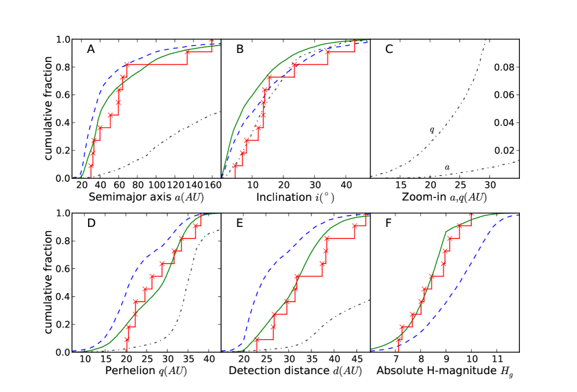
Figure 1: Cumulative distributions for 5 quantities, comparing the observed objects (red staircase) with the initially cold model’s simulated detections. The black dash-dot curves show the orbital model’s intrinsic $a,i$, $q$, and $d$ distributions. When coupled to two different $N(H_{g})$ distributions, the biases produce the differing predictions for the detections. A single power-law slope of $\alpha=0.8$ (blue dashed) is rejectable at $>$ 99% confidence in $d$, $q$ and $H_{g}$. Contrastingly, our preferred divot $N(H_{g})$ (green curve, see Fig. 2) provides vastly better matches, although both produce too many low-$i$ detections.

At any time some SOs are only $d$ = 20–30 AU away, allowing a 4-m telescope, in excellent conditions, to detect objects down to $H_{g}\sim 12$. For a monotonically increasing number distribution $N(H_{g})$, the abundant small objects at the observable volume’s innermost edge should dominate the detected sample. This is not what our survey found (Fig. 1), necessitating a relative lack of small SOs.

We discarded a sudden (ad-hoc) albedo change, as it would produce a gap in $H$-space, not a drop, which does not match the observations; the needed change is a sudden lack of $H_{g}>9$ (and therefore small) SOs.

2 Models

Several models of the SO orbital element distribution were exposed to the calibrated observational biases of the Canada France Ecliptic Plane Survey (CFEPS) in order to quantitatively constrain the intrinsic $N(H_{g})$ distribution. Drawing SOs from an orbital distribution model, and selecting $H_{g}$ from a candidate $N(H_{g})$ distribution, the CFEPS survey simulator (Jones et al., 2006) determines each object’s observability and produces a set of “simulated detections” expected from the model.

Two different SO orbital models are from a modified version of Kaib et al. (2011b) (henceforth KRQ11). KRQ11 focuses on the effects of solar migration in the Milky Way on Oort Cloud structure. While this is not the focus of the current work, we can use the KRQ11 control calculations, which assume an unchanging local galactic environment.

To test the sensitivity of our results to the dynamical context, we performed the same analysis on an independent model. Gladman & Chan (2006) modelled the scattering of objects in an initial Solar System having an additional planet of order Earth mass. As previously reported (Petit et al., 2011) this model also (perhaps surprisingly) satisfactorily represents the current SO ($a,q$) distribution, although too “cold” in inclinations. In fact, this model and the cold KRQ11 model produced very similar results, showing that our conclusions are mostly insensitive to the assumed Solar System history. Objects currently in the Centaur and detectable SO region (mostly $a<$200 AU) have, unsurprisingly, almost forgotten their initial state except for the the inclination distribution; the current SO orbital distribution is not diagnostic of the number and position of the planets early in the Solar System’s history.

3 Observations

CFEPS provided a set of detections of outer Solar System objects in a precisely calibrated survey (Jones et al., 2006; Kavelaars et al., 2009) whose pointing history, detection efficiency, and tracking performance were recorded. The final set of TNO detections (with full high-precision orbits) and the fully calibrated pointing history make up the L7 release (Petit et al., 2011). This absolute calibration of CFEPS allows a model of the present orbital (and size) distribution of to be passed through the CFEPS Survey Simulator, yielding a set of simulated detections whose orbital and $H_{g}$ distributions can be compared to the real detections.

The three models provide orbital distributions of all TNOs. The “scattering” TNOs are then selected out of the final 10 Myr stage of the model integrations using the criteria: variation of $a>$1.5 AU in semimajor axis during 10 Myr, with $a<1000$ AU (Morbidelli et al., 2004; Gladman et al., 2008). Historically, a simple $q$ cut was used to isolate the “scattered disk” (Duncan & Levison, 1997; Luu et al., 1997; Trujillo et al., 2000), which has serious disadvantages when trying to discuss the cosmogony, as there is a nearly impossible distinction between implanted (and thus scattered) and the original Kuiper Belt population (if any). Perihelion divisions also undesirably includes resonant objects and most inner main-belt TNOs.

The CFEPS SO sample consists of 9 objects (Table 1), supplemented by two SOs discovered in a high-latitude extension survey (covering $\simeq 470$ sqdg in 2007–2008, extending up to 65^∘ ecliptic latitude), which was fully calibrated in the same way as CFEPS.

To characterize the form of the $N(H_{g})$, we introduce a novel formulation, allowing for the exploration of distributions with knees and divots (a sudden drop in the differential number of objects followed by a recovery). We parameterised the $H_{g}$ distribution (Fig. 2A) with the fixed slope $\alpha_{b}=0.8$ (see below) for SOs brighter than a break at $H_{g}=9$ ($D\simeq$100 km), allowed an adjustable slope $\alpha_{f}$ for fainter objects, and an adjustable contrast $c\geq 1$.

The $H_{g}$-magnitudes are drawn from one of three types of distributions:

(1) a single exponential of logarithmic slope $\alpha$, (2) $N(H_{g}$) with a knee (contrast $c$ =1). That is, one slope $\alpha_{b}$ for SOs with $H_{g}<H_{knee}$ and $\alpha_{f}$ for $H_{g}>H_{knee}$, where $N(H_{g})$ is continuous across the knee at $H_{knee}$ and negative slopes $\alpha_{f}$ are allowed as suggested (Bernstein et al., 2004), and (3) one slope $\alpha_{b}$ to a divot at $H_{divot}$, which is a sudden drop in differential number by a factor $c$, with a potentially different slope $\alpha_{f}$ beyond the cliff at $H=H_{divot}$. Although in reality the discontinuity is unlikely to be an instantaneous drop, our data do not merit trying to constrain the values of the expected steep negative slope and small extent over which it drops; collisional models (Fraser, 2009; Campo Bagatin & Benavidez, 2012) do show collisional divots where the drop occurs over $D$ ranges of factors $<2$ (a few tenths of magnitude in $H_{g}$).

In principle there are four parameters: $\alpha_{b}$, $\alpha_{f}$, $H_{divot}$, and $c$ (Fig. 2). For $H_{g}<9$ a single power-law of $\alpha_{b}\simeq 0.8$ does indeed match our detections; we elected to fix this slope at that value with the unifying philosophy that all the hot transneptunian populations share this same hot slope; $\alpha_{b}=0.8$ matches both the hot Classical belt measured down to $H_{g}\simeq 8.0$ (Petit et al., 2011; Fraser & Kavelaars, 2008; Fuentes & Holman, 2008), and to the 3:2 resonators measured down to $H_{g}\simeq 9.0$ (Gladman et al., 2012). Our detections require a transition around $H_{g}=$9–10 to explain the relative lack of small detections; we thus fixed the knee/divot for our analysis at $H_{g}=9$ (slightly larger than $D$=100 km for 5% $g$-band albedo). This leaves only two free parameters: the contrast $c$ at the divot and the slope $\alpha_{f}$ for absolute magnitudes fainter than the divot/knee.

To assess a match, the Anderson-Darling (AD) statistic is calculated between our 11-object sample and the distribution of simulated detections from the model, for each orbital parameter. An AD significance level of $<5\%$ rejects the hypothesis that the real SO observations could be drawn from the simulated detections at the $95\%$ confidence level (for that orbital parameter). To retain a model, we required that none of the $q$, $d$, $i$, and $H_{g}$ distributions are rejectable at $>95\%$ confidence.

4 Absolute Magnitude Distribution

The observational bias is strong (Fig. 1) , but when accurately calibrated allows us to constrain the $H_{g}$ distribution’s form. Single power-laws predict significantly more close-in detections than were seen by CFEPS; for a slope of $\alpha=0.8$, roughly half of the expected detections (Fig. 1 D’s blue dashed curve) should have a distance at detection $d<$ 23 AU, which is the closest real SO in our sample. The observationally biased models predict that the majority of detected SOs would have orbits with $q<$20 AU at $d$ = 20–25 AU and be small ($H_{g}>9$ or $D\leq 100$ km) objects, in contrast to our detections, which demonstrates that our observations are sensitive beyond the break. When confined to $q>25AU$ (where objects must be large to be seen) the orbital models provide good matches, however extensions to smaller distance fail when using a single power-law, pointing to a breakdown arising from the the assumed $N(H_{g})$.

We rule out a single power-law of slope 0.8 at 99% confidence, and can rule out all single power-laws with slope between 0 and 1.2 at 95% confidence. Slopes of 0.5 and 0.6 are not rejectable across the whole distribution, but are rejectable (95% confidence) when the distribution is considered in both $H_{g}>9$ and $H_{g}<9$ subsets; we demand these work because the steep slopes measured for other hot populations match our $H_{g}<9$ detections well, and a shallower slope is erroneously found by measuring across a divot feature when requiring a single slope (see below).

Our relatively small sample is powerful because our detected SOs span the break and, when coupled with the precise CFEPS calibration, allows the non-detection of $H_{g}=$10-12 SOs (several magnitudes past the divot) to provide a strong constraint on $N(H_{g})$. Down to this limit, CFEPS detected moving objects as close as 20 AU with no rate of motion dependence. Because our orbits are accurate, we can separate the SOs from the other hot populations, and use a dynamical model specific to the SOs.

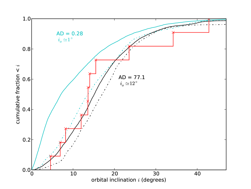
Figure 3: The hot (black dashed) and cold (light blue dashed) KRQ11 intrinsic $i$ distributions produce the biased distributions (solid lines) from our preferred model for comparison with the CFEPS sample (red). The hot model significantly improves the match because it has a relative lack (at the current epoch) of low-$i$ SOs to be detected by the survey; the eleven CFEPS SOs have $<1$% probability of being drawn from the initially cold simulation.

All of our $N(H_{g})$ cases have the obvious and previously-known problem that the model’s orbital inclinations are mostly lower than the true population’s (Petit et al., 2011; Gladman et al., 2012), even for the cases where the $N(H_{g})$ otherwise provides a good match. For example, Fig. 1 shows a divot ($c\simeq 6$, $\alpha_{f}$ = 0.5) producing a good match between the model’s expected detections (green curve) and the real SO sample (red), excepting the $i$ problem. Models (Levison et al., 2008) which scatter out a cold TNO population (from $d<30$ AU with initial inclination distribution widths $\sigma_{i}\leq 6^{\circ}$) to eventually form today’s hot population produce current TNO populations where too many low-$i$ detections are expected in observational surveys (Fig. 1B). This is part of growing evidence that the original planetesimal disk supplying today’s high-$i$ objects must have already been vertically excited before being scattered out (Petit et al., 2011; Gladman et al., 2012; Brasser & Morbidelli, 2012), which has strong cosmogonic implications for an extended quiescent phase of the early Solar System (Levison et al., 2008). We therefore computed a new SO model with a hotter ($\sigma_{i}\simeq 12^{\circ}$) initial disk; this provides an excellent match with today’s SO $i$-distribution (see Fig. 3) and we constrain $N(H_{g})$ below using this model.

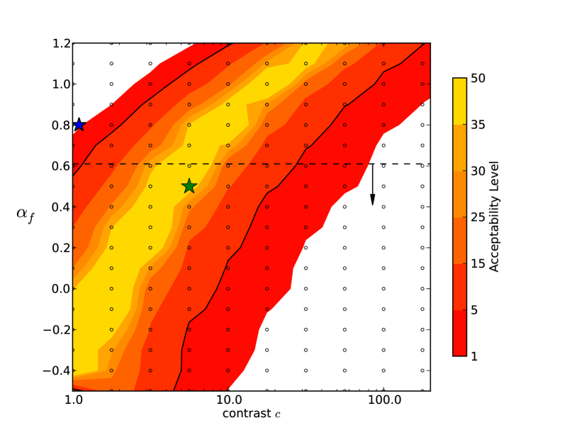
Figure 4: Contour values (colours) computed from a grid (points) in ($c,\alpha_{f}$) space, giving the Anderson-Darling probability of drawing the most rejectable of the $d$, $q$, $i$, and $H_{g}$ distributions from the hot KRQ model of today’s SOs. White areas indicate when the ($c$,$\alpha_{f}$) pair had $<$1% probability of coming from the model, and the black contour bounds $<$5%. A single power-law (blue, darker star) is rejected. Our favoured model (green, lighter star) satisfies both (a) $\alpha_{f}\simeq 0.5$ like known JFCs, (b) $\alpha\leq 0.6$ which prevents the extrapolated mass of small SOs from diverging.

To constrain the size distribution, a grid of possible divot contrasts and post-divot slopes was explored. Fig. 4 shows acceptability levels for the range of explored parameter pairs ($c,\alpha_{f}$). A single power-law of $\alpha=0.8$ (blue star Fig. 4) has $<1$% probability. We are left with a range of acceptable parameter space, including knee ($c$=1) and divot ($c>$1) scenarios; we further constrain $N(H_{g})$ by looking to other Kuiper Belt populations.

The so-called hot Kuiper Belt populations (the hot main belt, inner belt, resonant, and detached TNOs) share an $i$ distribution half-width of roughly $15^{\circ}$ (Petit et al., 2011) with the SOs, suggesting a cosmogonic link. In analyses of deep luminosity functions dominated by hot main-belt detections, the common conclusion (Bernstein et al., 2004; Fuentes et al., 2010) was that for magnitude $g>25$ the slope must break to a faint $\alpha_{f}<0.3$ value or even become negative in order to explain the lack of detections in the following few magnitudes; beyond this no data exists for the main Kuiper Belt. For SOs and their companion objects (Centaurs), however, many $H_{g}\gg 9$ objects are known from wide-field surveys, mostly detected at $d<20$ AU. In fact, measurements of Jupiter Family Comets (JFCs) in the $H_{g}\approx$14–17 range give slopes $\alpha_{f}\simeq 0.5\pm 0.1$ (see Table 6 of Solontoi et al. (2012)). These two arguments mean the SO distribution cannot remain at $\alpha_{f}<0.3$. leading us to discard knees to negative slopes. A divot can explain both a relative lack of objects beyond the break and the eventual recovery necessary to provide the JFCs. A divot also motivates the negative slopes measured, as a realistic divot will take the form of a decrease at the break, rather than the sharp discontinuity we use. We prefer the divot solution with $\alpha_{f}=$0.5 and $c\simeq$6 (green star Fig. 4) which matches the observations and allows for a single slope $\alpha_{f}=0.5$ from the divot out to the $H_{g}>$14 Jupiter Family comets whose slope is near the collisional equilibrium value (O’Brien & Greenberg, 2005).

5 External Arguments

As the hot populations have similar colours and $D>100$-km size distributions, it seems likely that they were all transplanted to join a pre-existing cold Kuiper Belt (Petit et al., 2011) during a common event early in the Solar System’s history, and would thus logically share the same divot and small $D$ distribution. Such a transplant process can successfully implant TNOs in the stable Kuiper Belt (Levison et al., 2008; Batygin et al., 2011), although the resonant population ratios and $i$ distribution are problematic (Gladman et al., 2012). We thus look for evidence of such a feature in other hot populations.

5.1 The Neptune Trojans

A search for Neptune Trojans (Sheppard & Trujillo, 2010) provided significant evidence that an $\alpha\sim 0.8$ power-law cannot continue for $D<$ 100-km Trojans; a divot was not apparent because Trojans significantly smaller were not detected. The dispersed Trojan inclination distribution (Sheppard & Trujillo, 2006), although not yet precisely measured, links these objects to all the other resonant populations (Gladman et al., 2012). Sheppard & Trujillo (2010) used Neptune Trojan searches to argue that beyond $m_{R}\simeq$23 (corresponding to $H_{g}\simeq 9$) there was an absence of Trojans due to non-detections, and thus smaller Trojans were missing. Assuming that the Trojans and other resonant TNOs were implanted from a scattering population, and thus share the same size distribution, we confirmed that our divot $N(H_{g})$ matches the lack of $D<$100 km Neptune Torjan detections in the Sheppard & Trujillo (2010) surveys.

Given our analysis, the conclusion would not be that small Neptune Trojans are “missing”, but rather that the sudden drop results in the population fainter than the divot not recovering in on-sky surface density until at least $H_{g}>11$, by which point the deepest survey lacked the sensitivity to detect them. If correct, detection of several small ($H_{g}>11$) Trojans requires surveying $\sim 100$ square degrees to 26th magnitude at the correct elongation.

5.2 Hot Populations

A recent deep telescopic survey (Fraser et al., 2010) estimated $\alpha\simeq 0.40\pm 0.15$ (within error of our preferred $\alpha_{f}$ = 0.5) from the apparent-magnitude distribution for “close” ($30<d<38$) TNOs (orbits were not obtained). These distances are dominated by several hot populations, but the measurement is shallower than the usual hot population slope of 0.8. We calculated $H_{g}$ magnitudes for the Fraser et al. (2010) detections and find that due to the survey’s depth, this sample is dominated by $H_{g}>9$ TNOs and thus would measure the post-divot slope.

6 Feasibility of a Divot

A primordial size-distribution wave at small sizes ($D$ = 2 km) could propagate (Fraser, 2009) to $D\sim$100 km in a dynamically hot ($\Delta v=2$ km/s) collisional environment after 500 Myr. Alternately, recent modeling of planetesimal creation (Johansen et al., 2007; Morbidelli et al., 2009), suggests that the protosolar nebula may only have produced planetesimals larger than a certain critical diameter, in which case the $\alpha_{b}=0.8$ slope and the $D\sim 100$ km divot size are set by planetesimal formation physics; smaller objects appear only later due to collisional fragmentation. These scenarios match our results, where one interprets the hot population’s $N(H_{g})$ to have been “frozen” when suddenly transplanted (scattered) from a denser region nearer the Sun to the large volume it now occupies, ending the collisional evolution. An exciting prospect is that the divot directly records a preferential $D$ that planet building produced in the solar-nebula region where the hot TNOs originally formed, and that the divot’s depth (which could easily range from $c$=2–30) measures the integrated collisional evolution (depending on both the duration of the pre-scattering phase and the random speeds present). An initial distribution with no $D<$100 km TNOs was shown (Campo Bagatin & Benavidez, 2012) to evolve into a divot with $c\sim$ 20 and $\alpha_{f}\simeq 0.5$, in the dynamical environment of the Nice model; such a 500-Myr quiescent phase (Gomes et al., 2005) allows a divot to form but the evidence we find for a higher-$i$ early phase may argue instead for a much shorter and more intense collisional environment.

Our divoted $N(H_{g})$ produces a cumulative distribution (Fig. 2 B) with a shallow plateau for $H_{g}$=9–12, similar to that deduced for the hot population and SOs in deep HST observations (Bernstein et al., 2004; Volk & Malhotra, 2008) and estimated for scattering impactors of the saturnian moons (Minton et al., 2012). Our estimate of $2\times 10^{6}$ SOs with $H_{g}<13$ and a slope of $\alpha_{f}=0.5$ extrapolates to $\sim 2\times 10^{9}$ SOs with $H_{g}<$18, providing a sufficient number (Duncan & Levison, 1997; Volk & Malhotra, 2008) of SOs to feed the Jupiter Family Comets, while satisfying the observed plateau.

Single power-laws that fit the $H_{g}<9$ SOs fail when extended to smaller objects. Our novel divot parameterisation (Fig. 2) matches our data and would simultaneously explain the puzzles of the JFC source, the “missing” Neptune Trojans, and the known rollover in the Kuiper Belt’s luminosity function. To better constrain the form of the break, a new survey must find and determine orbits for $\sim$10 SOs from 10–30 AU; this requires discovery (and tracking over several degrees of arc) targets moving up to 15”/hr by observing $\sim$200 sq. deg. to 24th magnitude.

Facilities: CFHT, NRC (HIA)

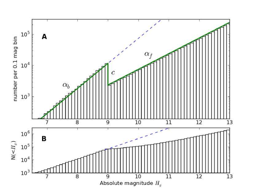
Figure 2: Histograms of the $N(H_{g})$ distribution for our preferred divot solution. The vertical axes show the total SO numbers using the absolute CFEPS calibration (Petit et al., 2011). A: The differential distribution (solid green), with an extrapolated $\alpha=$ 0.8 beyond $H_{g}$ = 9 (dashed blue). The contrast $c\simeq 6$ is the ratio of differential number on either side of the divot. B: The cumulative version. For $H_{g}>$13 the cumulative $N(<H_{g})$ has reached slope $\alpha_{f}$ after the flattened region following the divot.

Designation	a (AU)	q (AU)	i (deg)	d (AU)	Hg
L4k09	30.19	24.60	13.586	26.63	9.5
HL8a1	32.38	22.33	42.827	44.52	7.3
L4m01	33.48	28.73	8.205	31.36	8.9
L4p07	39.95	26.31	23.545	29.59	7.7
L3q01	50.99	33.41	6.922	38.17	8.1
L7a03	59.61	22.26	4.575	46.99	7.1
L4v11	60.04	31.64	11.972	26.76	10.0
L4v04	64.10	38.10	13.642	31.85	9.1
L4v15	68.68	36.81	14.033	22.95	9.0
L3h08	159.6	20.26	15.499	38.45	8.0
HL7j2	133.25	20.67	34.195	37.38	8.4

Table 1: CFEPS + extension SO sample

References

- Bernstein et al. (2004) Bernstein, G.M. et al. 2004, AJ, 128, 1364
- Brasser & Morbidelli (2012) Brasser, R. & Morbidelli, A. 2012 Asteroids, Comets, and Meteors meeting, abstract.
- Batygin et al. (2011) Batygin, K., Brown, M. & Fraser, W. 2011, ApJ, 13, 738
- Campo Bagatin & Benavidez (2012) Campo Bagatin & A.,Benavidez, P. 2012, MNRAS, 423, 1254
- Duncan & Levison (1997) Duncan, M. & Levison, H.F. 1997, Science, 276, 1670
- Elliot et al. (2005) Elliot, J., Kern, S.D. & Clancy, K.B. 2005, AJ, 129, 1117
- Fraser (2009) Fraser, W. 2009, ApJ, 706, 119
- Fraser et al. (2010) Fraser, W., Brown, M. & Schwamb, M. 2010, Icarus, 210, 944
- Fraser & Kavelaars (2008) Fraser, W. & Kavelaars J.J. 2008, Icarus, 198, 452
- Fraser & Kavelaars (2009) Fraser, W. & Kavelaars, J.J. 2009, AJ, 137, 72
- Fuentes & Holman (2008) Fuentes C., & Holman, M. 2008, AJ, 136, 83
- Fuentes et al. (2010) Fuentes, C., Holman, M., Trilling, D. & Protopapas, P. 2010, ApJ, 722, 1290
- Gladman et al. (2001) Gladman, B. et al. 2001, AJ, 122, 1051
- Gladman & Chan (2006) Gladman, B. & Chan, C. 2006, ApJ, 643, L135
- Gladman et al. (2009) Gladman, B., Kavelaars, J.J., Petit, J.-M., et al. 2009, ApJ, 697, L91
- Gladman et al. (2012) Gladman, B., Lawler, S., Petit, J.-M, et al. 2012, AJ, 144, 23
- Gladman et al. (2008) Gladman, B., Marsden, B.G. & Vanlaerhoven, C. 2008, in The Solar System Beyond Neptune 43
- Gomes et al. (2005) Gomes, R., Levison,H.F., Tsiganis & K., Morbidelli, A. 2005, Nature, 435, 466
- Jewitt et al. (1988) Jewitt, D., Luu, J., & Trujillo, C. 1988, AJ115, 2125
- Johansen et al. (2007) Johansen, A., Oishi, J., Mac Low, M.-M., et al. 2007, Nature, 448, 1022
- Jones et al. (2006) Jones, R.L., Gladman, B., Petit, J.-M., et al. 2006, Icarus, 185, 508
- Kaib et al. (2011a) Kaib, N., Quinn, T. & Brasser, R. 2011, ApJ, 141, 3
- Kaib et al. (2011b) Kaib, N., Ros̆kar, R. & Quinn, T. 2011, Icarus, 215, 491
- Kavelaars et al. (2009) Kavelaars, J.J., Jones, R.L, Gladman, B., et al. 2009, AJ, 137, 491
- Levison et al. (2001) Levison, H.F., Dones, L. & Duncan, M. 2001, AJ, 121, 2253
- Levison et al. (2008) Levison, H., Morbidelli, A., Van Laerhoven, C., Gomes, R. & Tsiganis, K. 2008, Icarus, 196, 258
- Luu et al. (1997) Luu, J., Marsden, B., Jewitt, D., et al. 1997, Nature, 387, 573
- Minton et al. (2012) Minton, D., Richardson, J., Thomas, P., Kirchoff, M. & Schwamb, M. 2012, in ACM Conf. Sess 551
- Morbidelli et al. (2009) Morbidelli, A., Bottke, W.F., Nesvorný, D. & Levison, H. 2009, Icarus, 204, 448
- Morbidelli et al. (2004) Morbidelli, A., Emel’yanenko, V. & Levison, H.F. 2004, MNRAS, 355, 935
- O’Brien & Greenberg (2005) O’Brien, D. & Greenberg, R. 2005, Icarus, 178, 179
- Petit et al. (2011) Petit, J.-M, Kavelaars, J.J., Gladman, B., et al. 2011, AJ, 142, 131
- Sheppard & Trujillo (2006) Sheppard, S. & Trujillo, C. 2006, Science, 313, 511
- Sheppard & Trujillo (2010) Sheppard, S. & Trujillo, C. 2010, ApJ, 723, L233
- Solontoi et al. (2012) Solontoi, M., Ivezić, Ž., Jurić, M. et al. 2012, Icarus, 218, 571
- Volk & Malhotra (2008) Volk, K. & Malhotra, R. 2008, ApJ, 687, 714
- Trujillo et al. (2000) Trujillo, C., Jewitt, D., & Luu, J. 2000, ApJ, 529, 103