A variational perspective on cloaking by anomalous localized resonance

Abstract

A body of literature has developed concerning “cloaking by anomalous localized resonance”. The mathematical heart of the matter involves the behavior of a divergence-form elliptic equation in the plane, $\nabla\cdot(a(x)\nabla u(x))=f(x)$. The complex-valued coefficient has a matrix-shell-core geometry, with real part equal to $1$ in the matrix and the core, and -1 in the shell; one is interested in understanding the resonant behavior of the solution as the imaginary part of $a(x)$ decreases to zero (so that ellipticity is lost). Most analytical work in this area has relied on separation of variables, and has therefore been restricted to radial geometries. We introduce a new approach based on a pair of dual variational principles, and apply it to some non-radial examples. In our examples, as in the radial setting, the spatial location of the source $f$ plays a crucial role in determining whether or not resonance occurs.

MSC: 35Q60, 35P05

Keywords: cloaking, anomalous localized resonance, negative index metamaterials

1 Introduction

A body of literature has developed concerning “cloaking by anomalous localized resonance”. Cloaking of two types of objects has been considered: (a) dipoles or inclusions, considered e.g. in [BrunoLintner, Nicorovici-etal1994, Milton-etal2005, Milton-etal2006, BouchitteSchweizer2010] and (b) spatially localized sources [Ammari-etal]. In this article we work in the setting of localized sources.

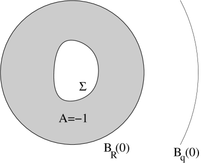
Figure 1: Sketch of the core-shell-matrix geometry.

Focusing initially on the math (not the physics), we are interested in a divergence-form PDE in the plane:

$$\nabla\cdot(a_{\eta}\nabla u_{\eta}) =f\quad\text{ on }\mathbb{R}^{2}$$ (1.1)

$$\ \ \nabla{u}_{\eta} \to 0\ \ {\rm as}\ |x|\to\infty.$$

The coefficient $a_{\eta}(x)$ is piecewise constant and complex-valued, with constant imaginary part $\eta>0$:

$$a_{\eta}(x)=A(x)+i\eta;$$ (1.2)

its real part has a matrix-shell-core character in the sense that

$$A(x)=\left\{\begin{array}[]{cl}+1&\mbox{outside $B_{R}(0)$}\\ -1&\mbox{in the shell $B_{R}(0)\setminus\Sigma$}\\ +1&\mbox{in the core $\Sigma$}\end{array}\right.$$ (1.3)

(see Figure 1). Concerning the core, we assume that

$$\Sigma\subset B_{1}(0)$$ (1.4)

so the shell includes an annulus of width $R-1$. Concerning the source $f$, we assume it is real-valued, supported at distance $q$ from the origin, and has zero mean:

$$f=F\,\mathcal{H}^{1}\lfloor\partial B_{q}(0),\quad F:\partial B_{q}(0)\to\mathbb{R},\ F\in L^{2}(\partial B_{q}(0)),\text{ and }\int_{\partial B_{q}(0)}F\,d\mathcal{H}^{1}=0\,.$$ (1.5)

Our interest lies in the question:

Question: As $\eta\rightarrow 0$ with $f$ and $A(x)$ held fixed, what is the behavior of

$$E_{\eta}:=\frac{\eta}{2}\int_{\mathbb{R}^{2}}|\nabla u_{\eta}|^{2}\,dx\ ?$$

In the radial setting, i.e. when $\Sigma=B_{1}(0)$, one expects by analogy with [Ammari-etal, BouchitteSchweizer2010, Milton-etal2006, Milton-etal2005, Nicorovici-etal1994] that the answer depends mainly on the location of the source. Specifically: there is a critical radius $R^{*}=R^{3/2}$ such that for a broad class of sources $f$,

$$\limsup_{\eta\rightarrow 0}E_{\eta}=\infty q<R^{*}$$ if , while

$$\limsup_{\eta\rightarrow 0}E_{\eta}<\infty \mbox{ if $q>R^{*}$}.$$

Note that it is no restriction to fix the core radius to be $1$. A scaling argument implies that, for core radius $r_{0}$, and shell radius $R$, the critical radius is

$$R^{*}\,=\,r_{0}\left(\frac{R}{r_{0}}\right)^{3/2}=\left(\frac{R}{r_{0}}\right)^{1/2}R.$$

Definition 1.1 (Resonance).

Let a configuration be given by coefficients $A$ and source $f$ as in (1.3)–(1.5). We shall call the configuration resonant, if

$$\limsup_{\eta\to 0}E_{\eta}\ =\ \infty\,.$$

Otherwise we call the configuration non-resonant.

In the physics literature the term “anomalous localized resonance” is used. An anomalous feature of the resonance is that it is not associated to a finite dimensional eigenvalue of a linear operator and a forcing term at or near the resonant frequency. Instead, the resonance here is associated to an infinite dimensional kernel of the limiting (non-elliptic) operator. The word localized refers to the fact that the resonance is spatially localized: while $\int|\nabla u_{\eta}|^{2}\rightarrow\infty$ if $q<R^{*}$, the potential $u_{\eta}$ (and therefore also its gradient $\nabla u_{\eta}$) stay uniformly bounded outside some ball.

The connection to cloaking is as follows (see [Ammari-etal] for a more thorough discussion). For time-harmonic wave propagation in the quasistatic regime, $E_{\eta}$ is the rate at which energy is dissipated to heat. Let us now consider a source $\alpha_{\eta}f$, where $\alpha_{\eta}\in\mathbb{R}$ is a scaling factor. If the (unscaled) source $f$ produces resonance (i.e. if $E_{\eta}\rightarrow\infty$) then the source $\alpha_{\eta}f$ is connected to the energy dissipation $\alpha_{\eta}^{2}E_{\eta}$. If the physical source $\alpha_{\eta}f$ has finite power, then we must have $\alpha_{\eta}\rightarrow 0$ as $\eta\to 0$. If the fields $u_{\eta}$ associated with the unscaled source $f$ are bounded outside a certain region, then the physical fields $\alpha_{\eta}u_{\eta}$ vanish in that region as $\eta\to 0$. This implies that the finite power source $\alpha_{\eta}f$ is not visible from outside.

Returning to a more mathematical perspective: we are interested in this problem because it involves the behavior of the elliptic system (1.1) in a limit when ellipticity is lost. It is not surprising that oscillatory behavior occurs in such a limit. It is however surprising that, at least in the radial examples, (a) resonance depends so strongly on the location of the source, and (b) the oscillatory behavior is spatially localized. We would like to understand the following question:

Question: Is this surprising behavior particular to the radial setting, or is it a more general phenomenon?

The present paper addresses only point (a): the dependence on the location of the source. Our method, which is variational in character, is unfortunately not well-suited to the study of point (b).

We know only one numerical study of a similar problem with non-radial (and non-slab) geometry. The paper [BrunoLintner] by Bruno and Lintner considered, via numerical simulation, various examples including an elliptical core in an elliptical shell. The results were similar to those of the radial case; in particular, the structure seemed to cloak a polarizable dipole placed sufficiently near the shell.

The paper [Ammari-etal] by Ammari et al considers a problem very similar to ours. The main difference is that both the outer and inner edges of the shell are not constrained to be radial. (There is also a minor difference: their PDE has $a_{\eta}=1$ in the matrix and core and $a_{\eta}=-1+i\eta$ in the shell, so energy is dissipated only in the shell.) Using a representation based on single layer potentials, Ammari et al obtain an expression for a spatially localized analog of $E_{\eta}$. To make use of their expression, one needs detailed information on the spectral properties of certain boundary integral operators. This information is difficult to come by in general and hence, beyond the radial setting, it is unclear how to use their method to obtain information on resonance and non-resonance in the limit as $\eta\rightarrow 0$.

Our approach is based on variational principles. The starting point is a pair of (dual) variational principles for $E_{\eta}$. One expresses $E_{\eta}$ as a minimum; trial functions may be used to provide an upper bound in order to show that resonance doesn’t occur. The dual principle expresses $E_{\eta}$ as a maximum; trial functions may be used to provide a lower bound in order to show that resonance occurs. Similar variational principles were considered in [CherkaevGibiansky, Milton-Seppecher-Bouchitte]. Our main results – all proved using the variational principles – are the following:

1. If there is no core then there is always resonance, for any source radius $q>R$ and any nonzero $f$ (see Proposition 3.2).

2. For any core $\Sigma\subset B_{1}(0)$, there is resonance for a broad class of sources $f$, provided the source location is $q<R^{*}:=R^{3/2}$ (see Theorem 3.4).

3. In the radial case (when $\Sigma=B_{1}(0)$), $R^{*}:=R^{3/2}$ is critical, in the sense that (a) when the source location is $q<R^{*}$ resonance occurs for a broad class of $f$’s, and (b) when the location is $q>R^{*}$ resonance does not occur for any $f$ (see Theorem 3.4 and Proposition 4.1).

4. In the (weakly) nonradial case when the core is $B_{\rho}(z_{0})$ with $|z_{0}|$ sufficiently near $0$ and $\rho$ sufficiently near $1$, resonance does not occur if the source location $q$ is sufficiently large (see Theorem 5.3).

Point (iii) is already known, from Section 5 of [Ammari-etal]. Our variational method is interesting even in this radial setting: our proof of (iii) is, we think, simpler and more elementary than the argument of [Ammari-etal]. Unfortunately, our methods do not seem to provide simple proofs for the localization effect when there is resonance.

In focusing on (1.1), we have chosen the imaginary part of $a_{\eta}$ to be the same constant constant in the matrix, shell, and core. This simplifies the formulas, and it seems physically unobjectionable. But we suppose a similar method could be used when the imaginary part is different in each region.

We specifically consider sources $f$ that are concentrated on the curve $\partial B_{q}(0)$. Our method also allows the study of more general distributions of sources, which can be obtained as a superpositions of concentrated sources, $f$, at different values of $q$.

We have taken the core to have $A(x)=1$ because this case has particular interest: in the radial setting, the “cloaking device is invisible” if the core has $A=1$, see [Nicorovici-etal1994]. However anomalous localized resonance also occurs when $A$ takes a different (constant) value in the core. It would be interesting to extend our method to analyze cores with $A\neq 1$.

Our assumption that $A(x)=-1$ in the shell is essential to the phenomenon. Indeed, our PDE problem becomes very different if the ratio across each interface, the plasmonic eigenvalue, is different from $-1$. This can be seen from the perspective of the boundary integral method, where ratios other than $-1$ lead to boundary integral equations of Fredholm type, see [Ammari-etal, Grieser:12]

Our main results are almost exclusively for a circular outer shell boundary $\partial B_{R}(0)$. This is essential to our method, since we use the perfect plasmon waves on the outer shell boundary in the construction of comparison functions. We refer to Section 3 for a further discussion. A more general geometry is only treated in Proposition 3.3 with the help of a domain transformation. Related techniques are used in [Nguyen:12].

Plasmonic resonance effects have many potential applications. This is one of the reasons why the development of negative index metamaterials is another much-studied research area, see e.g. [BouchitteSchweizer-Maxwell, Milton-etal2007, Pendry2004]. We hope that our variational approach will be useful also in the other contexts.

Notation.

We use polar coordinates and write $x\in\mathbb{R}^{2}$ as $x=r\,(\cos\theta,\sin\theta)$. In Section 5 we identify $\mathbb{R}^{2}\equiv\mathbb{C}$ via $(x_{1},x_{2})\equiv x_{1}+ix_{2}=z$. With this notation, we identify $z=re^{i\theta}$. The complex conjugate of $z$ is denoted by $\overline{z}$.

We denote the sphere with radius $\rho$, centered at $x_{0}$, as $B_{\rho}(x_{0})$. The measure $\mathcal{H}^{1}\lfloor\partial\Omega$ is the $1$-dimensional Hausdorff measure on the curve $\partial\Omega$. Unless otherwise specified, integrals are over all of $\mathbb{R}^{2}$. Constants $C$ may change from one line to the next.

2 The primal and dual variational principles

In the subsequent definitions of energies we always consider the source $f$ as a given element $f\in H^{-1}(\mathbb{R}^{2})$. We will always consider sources with a compact support (in the sense of distributions). Furthermore, we shall assume that the sources $f$ have a vanishing average,

$$\int_{\mathbb{R}^{2}}\,f=0.$$

Since $f$ is merely a distribution, it would be more correct to write $\langle f,\mathrm{\bf 1}\rangle=0$, where $\mathrm{\bf 1}:\mathbb{R}^{2}\to\mathbb{R}$ is the constant function, $\mathrm{\bf 1}(x)=1$ for all $x\in\mathbb{R}^{2}$. We note that since $f$ has compact support, it can be applied to test-functions that are only locally of class $H^{1}$.

We remark that, while the main results of this paper concern $\mathbb{R}^{2}$, the primal and dual variational principles generalize to any dimension.

2.1 A complex elliptic system and its non-elliptic limit

Our aim is to study, for a sequence $\eta=\eta_{j}\to 0$, sequences $u_{\eta}$ of solutions to (1.1). For non-vanishing dissipation, $\eta\neq 0$, (1.1) is an elliptic PDE, while the system loses ellipticity in the limit $\eta\to 0$.

To a solution $u_{\eta}:\mathbb{R}^{2}\to\mathbb{C}$ of the original complex-valued equation

$$\nabla\cdot(a_{\eta}\nabla u_{\eta})=f$$ (2.1)

we have associated an energy $E_{\eta}$ (in physical terms the energy dissipation in the structure)

$$E_{\eta}(u_{\eta}):=\frac{\eta}{2}\int_{\mathbb{R}^{2}}|\nabla u_{\eta}|^{2}\,.$$ (2.2)

As noted in the introduction, the phenomenon of cloaking is related to resonance in the sense of Definition 1.1,

$$E_{\eta}(u_{\eta})\to\infty$$ (2.3)

along a subsequence $\eta\searrow 0$.

We can write the complex scalar equation for $u_{\eta}:\mathbb{R}^{2}\to\mathbb{C}$ as a system of two real scalar equations. We set

$$u_{\eta}=v_{\eta}+i\,\frac{1}{\eta}\,w_{\eta},\quad\text{ with }v_{\eta},w_{\eta}:\mathbb{R}^{2}\to\mathbb{R}.$$ (2.4)

For a real-valued source, $f:\mathbb{R}^{2}\to\mathbb{R}$, the complex equation $\nabla\cdot(a_{\eta}\nabla u_{\eta})=f$ with $a_{\eta}=A+i\eta$ is equivalent to the coupled system of two real equations on $\mathbb{R}^{2}$,

$$\nabla\cdot(A\nabla v_{\eta})-\Delta w_{\eta} =f,$$ (2.5)

$$\nabla\cdot(A\nabla w_{\eta})+\eta^{2}\Delta v_{\eta} =0.$$ (2.6)

The energy $E_{\eta}(u_{\eta})$ can be expressed in terms of $v_{\eta}$ and $w_{\eta}$ as

$$E_{\eta}(u_{\eta})=\frac{\eta}{2}\int|\nabla u_{\eta}|^{2}=\frac{\eta}{2}\int|\nabla v_{\eta}|^{2}+\frac{1}{2\eta}\int|\nabla w_{\eta}|^{2}.$$ (2.7)

In the following subsections we introduce

1. the primal variational problem, a minimization problem, which characterizes the energy $E_{\eta}(u_{\eta})$ as a constrained minimum; and

2. the dual variational problem, a maximization problem, which characterizes the energy $E_{\eta}(u_{\eta})$ as a constrained maximum.

To provide a functional analytic framework for the study of the variational problems we introduce the following function space of real or complex-valued functions,

$$\dot{H}^{1}(\mathbb{R}^{2}):=\left\{U\in L^{2}_{\mathrm{loc}}(\mathbb{R}^{2})\left|\nabla U\in L^{2}(\mathbb{R}^{2})\right.\right\},\quad\|U\|_{\dot{H}^{1}(\mathbb{R}^{2})}^{2}:=\int_{\mathbb{R}^{2}}|\nabla U|^{2}+\int_{B_{1}(0)}|U|^{2}\,.$$ (2.8)

2.2 The primal variational problem

For fixed $f\in H^{-1}(\mathbb{R}^{2})$ we consider the energy functional

$$I_{\eta}(v,w):=\frac{\eta}{2}\int|\nabla v|^{2}+\frac{1}{2\eta}\int|\nabla w|^{2}\,$$ (2.9)

defined for $v,w\in\dot{H}^{1}(\mathbb{R}^{2})$. The primal variational problem is given by

$$\begin{split}&{\rm minimize}\ I_{\eta}(\tilde{v},\tilde{w})\textrm{ over all pairs}\ (\tilde{v},\tilde{w})\\ &\text{which satisfy the PDE constraint }\nabla\cdot(A\nabla\tilde{v})-\Delta\tilde{w}=f\,.\end{split}$$ (2.10)

Lemma 2.1.

Let $f\in H^{-1}(\mathbb{R}^{2})$ be a fixed real-valued source with compact support and with vanishing average. Then the primal variational problem (2.10) is equivalent to the original problem (2.1) with energy (2.2) in the following sense.

1. The infimum

   $$\inf\left\{\ I_{\eta}(\tilde{v},\tilde{w})\ \middle|\ (\tilde{v},\tilde{w})\in\dot{H}^{1}(\mathbb{R}^{2})\times\dot{H}^{1}(\mathbb{R}^{2}),\ \ \nabla\cdot(A\nabla\tilde{v})-\Delta\tilde{w}=f\right\}$$ (2.11)

   is attained at a pair $(v_{\eta},w_{\eta})\in\dot{H}^{1}(\mathbb{R}^{2})\times\dot{H}^{1}(\mathbb{R}^{2})$.

2. The minimizing pair, $(v_{\eta},w_{\eta})$, is unique up to an additive constant. The function $u_{\eta}:=v_{\eta}+i\eta^{-1}w_{\eta}$ is the unique (up to an additive constant) solution of the original problem (2.1).

3. For the solutions, the energies coincide,

   $$E_{\eta}(u_{\eta})=I_{\eta}(v_{\eta},w_{\eta})\,.$$ (2.12)

Remark. The lemma implies

$$E_{\eta}(u_{\eta})\leq I_{\eta}(\tilde{v},\tilde{w})$$ (2.13)

for every pair $(\tilde{v},\tilde{w})$ that satisfies the PDE constraint of (2.10). We shall use the inequality (2.13) to establish non-resonance.

Proof.

Point 1. Fix a radius $s>0$ such that $\mathrm{supp}(f)\subset B_{s}(0)$, we introduce the function space with constraint:

$$X:=\left\{\tilde{u}\in\dot{H}^{1}(\mathbb{R}^{2})\ \middle|\ \int_{B_{s}(0)}\tilde{u}=0\right\}.$$

Note that $I_{\eta}$, defined in (2.9), is convex on $X\times X$. Moreover, the constraint set is non-empty. Indeed, choose $\tilde{v}_{*}$ smooth and of compact support and defined $\tilde{w}_{*}$ to be the weak solution of $\Delta\tilde{w}_{*}=-f+\nabla\cdot\left(A\nabla\tilde{v}_{*}\right)$. It follows that the infimum in (2.11) is attained on $X\times X$ (see, e.g., Chapter 8.2 of [Evans]), i.e. there exists $(v_{\eta},w_{\eta})\in X\times X$ such that

$$I_{\eta}(v_{\eta},w_{\eta})\leq I_{\eta}(\tilde{v},\tilde{w})\ \textrm{for all}\ (\tilde{v},\tilde{w})\in X\times X,\ {\rm with}\ \nabla\cdot(A\nabla\tilde{v})-\Delta\tilde{w}=f\,.$$

Point 2. We first observe that the constraint (2.10) is identical to (2.5). As a minimizer of $I_{\eta}$, the pair $(v_{\eta},w_{\eta})$ satisfies the Euler-Lagrange equation

$$\partial_{\tau}I_{\eta}\Big{(}v_{\eta}+\tau\tilde{v},w_{\eta}+\tau\tilde{w}\Big{)}\Big{|}_{\tau=0}\ =\ 0,\text{ for every }(\tilde{v},\tilde{w})\in X\times X$$

satisfying $\nabla\cdot(A\nabla\tilde{v})-\Delta\tilde{w}=0$. For the energy $I_{\eta}$, this equation reads

$$0=\eta\int\nabla v_{\eta}\cdot\nabla\tilde{v}+\frac{1}{\eta}\int\nabla w_{\eta}\cdot\nabla\tilde{w}=\eta\int\nabla v_{\eta}\cdot\nabla\tilde{v}+\frac{1}{\eta}\int\nabla w_{\eta}\cdot A\nabla\tilde{v},$$

where we have used the constraint to obtain the second equality. We find

$$-\frac{1}{\eta}\,\Big{\langle}\eta^{2}\Delta v_{\eta}+\nabla\cdot(A\nabla w_{\eta}),\tilde{v}\Big{\rangle}=0,\ \ \forall\,\tilde{v}\in X\ ,$$

which is the weak form of (2.6). We use here that $\tilde{v}$ can be any element of $\dot{H}^{1}(\mathbb{R}^{2})$ with compact support, since an associated $\tilde{w}\in\dot{H}^{1}(\mathbb{R}^{2})$ can be obtained as the solution of a Poisson problem. As a solution of (2.5)-(2.6), the pair $(v_{\eta},w_{\eta})$ defines through $u_{\eta}\equiv v_{\eta}+i\eta^{-1}w_{\eta}$ a solution of the original problem (2.1).

The uniqueness is a consequence of the fact that the original problem (2.1) possesses a unique solution. This can be seen from the Lax-Milgram Lemma. We introduce a sesquilinear form $b(\cdot,\cdot):X\times X\to\mathbb{C}$ defined by

$$b(\tilde{u}_{1},\tilde{u}_{2}):=-i\int_{\mathbb{R}^{2}}a_{\eta}\nabla\tilde{u}_{1}\overline{\nabla\tilde{u}_{2}}\,.$$

The form $b(\cdot,\cdot)$ is coercive on $X$

$$\Re b(\tilde{u},\tilde{u})\geq\ C\|\tilde{u}\|_{X}^{2}\ ,$$

since the imaginary part of $a_{\eta}$ is strictly positive and by the Poincaré inequality. Existence and uniqueness of a weak solution $u_{\eta}\in\dot{H}^{1}(\mathbb{R}^{2})$ solution follows from the Lax-Milgram Lemma.

Point 3. The energy equality (2.12) was already observed in (2.7).

The proof of Lemma 2.1 is complete. ∎

2.3 The dual variational problem

For fixed $f\in H^{-1}(\mathbb{R}^{2})$, we introduce the dual energy

$$J_{\eta}(v,\psi):=\int f\psi-\frac{\eta}{2}\int|\nabla v|^{2}-\frac{\eta}{2}\int|\nabla\psi|^{2}\ ,$$ (2.14)

defined for $(v,\psi)\in\dot{H}^{1}(\mathbb{R}^{2})$. The dual variational problem is given by

$$\begin{split}&\textrm{maximize}\ J_{\eta}(\tilde{v},\tilde{\psi})\ \textrm{over all pairs}\ (\tilde{v},\tilde{\psi})\\ &\text{which satisfy the PDE constraint }\nabla\cdot(A\nabla\tilde{\psi})+\eta\Delta\tilde{v}=0.\end{split}$$ (2.15)

The following lemma establishes that the dual variational problem is also equivalent to the original complex equation.

Lemma 2.2.

Let $f\in H^{-1}(\mathbb{R}^{2})$ be a fixed real-valued source with compact support and with vanishing average. Then the dual variational problem (2.15) is equivalent to the original problem (2.1) with energy (2.2) in the following sense.

1. The supremum

   $$\sup\left\{\ J_{\eta}(\tilde{v},\tilde{\psi})\ \middle|\ (\tilde{v},\tilde{\psi})\in\dot{H}^{1}(\mathbb{R}^{2})\times\dot{H}^{1}(\mathbb{R}^{2}),\ \ \nabla\cdot(A\nabla\tilde{\psi})+\eta\Delta\tilde{v}=0\right\}$$ (2.16)

   is attained at a pair $(v_{\eta},\psi_{\eta})\in\dot{H}^{1}(\mathbb{R}^{2})\times\dot{H}^{1}(\mathbb{R}^{2})$.

2. The maximizing pair, $(v_{\eta},\psi_{\eta})$, is unique up to an additive constant. The function $u_{\eta}:=v_{\eta}+i\psi_{\eta}$ is the unique (up to constants) solution of the original problem (2.1).

3. For the solutions, the energies coincide,

   $$E_{\eta}(u_{\eta})=J_{\eta}(v_{\eta},\psi_{\eta})\,.$$ (2.17)

Remark. The lemma implies

$$E_{\eta}(u_{\eta})\geq J_{\eta}(\tilde{v},\tilde{\psi})$$ (2.18)

for every pair $(\tilde{v},\tilde{\psi})$, which satisfies the PDE constraint of (2.15). We shall use inequality (2.18) to establish our results on resonance.

Proof.

Point 1. The existence of a maximizing pair $(v_{\eta},\psi_{\eta})$ for the variational problem (2.16) follows from the concavity of $J_{\eta}$ (convexity of $-J_{\eta}$), by arguments analogous to those given above for the primal variational problem.

Point 2. At a maximizer, $(v_{\eta},\psi_{\eta})$, one has for all $\tilde{v},\tilde{\psi}\in\dot{H}^{1}(\mathbb{R}^{2})\cap L^{2}(\mathbb{R}^{2})$ satisfying the PDE constraint $\nabla\cdot(A\nabla\tilde{\psi})+\eta\Delta\tilde{v}=0$, that

$$\partial_{\tau}J_{\eta}\Big{(}v_{\eta}+\tau\tilde{v},\psi_{\eta}+\tau\tilde{\psi}\Big{)}\Big{|}_{\tau=0}\ =\ 0.$$

For the energy $J_{\eta}$, this relation provides

$$\int f\tilde{\psi}-\eta\int\nabla v_{\eta}\cdot\nabla\tilde{v}-\eta\int\nabla\psi_{\eta}\cdot\nabla\tilde{\psi}\ =\ 0.$$ (2.19)

Using the PDE constraint $\nabla\cdot(A\nabla\tilde{\psi})+\eta\Delta\tilde{v}=0$ to replace $\tilde{v}$, we find that (2.19) is equivalent to

$$0 =\int f\tilde{\psi}+\int\nabla v_{\eta}\cdot A\nabla\tilde{\psi}-\eta\int\nabla\psi_{\eta}\cdot\nabla\tilde{\psi}$$

$$=\Big{\langle}f-\nabla\cdot(A\nabla v_{\eta})+\eta\Delta\psi_{\eta},\tilde{\psi}\Big{\rangle}\,.$$

We conclude that the pair $(v_{\eta},w_{\eta}):=(v_{\eta},\eta\psi_{\eta})$ is a weak solution of (2.5)-(2.6) and, thus, that $u_{\eta}:=v_{\eta}+i\psi_{\eta}$ is a solution of $\nabla\cdot\left(a_{\eta}\nabla u_{\eta}\right)=f$ on $\mathbb{R}^{2}$. Uniqueness follows again from the fact that $u_{\eta}$ is unique up to constants.

Point 3. Regarding the energy equality, we calculate

$$E_{\eta}(u_{\eta})-J_{\eta}(v_{\eta},\psi_{\eta}) =\frac{\eta}{2}\int|\nabla u_{\eta}|^{2}-J_{\eta}(v_{\eta},\psi_{\eta})=\eta\int|\nabla v_{\eta}|^{2}+\eta\int|\nabla\psi_{\eta}|^{2}-\int f\psi_{\eta}$$

$$=-\int\nabla v_{\eta}\cdot A\nabla\psi_{\eta}-\Big{\langle}\psi_{\eta},-f+\nabla\cdot(A\nabla v_{\eta})\Big{\rangle}-\int f\psi_{\eta}=0.$$

This concludes the proof of Lemma 2.2. ∎

3 Resonance results

As discussed in the introduction, we consider configurations of the following type:

1. The coefficients $a_{\eta}(x)$ and $A(x)$ are defined by (1.2)-(1.3) with core $\Sigma\subset B_{1}(0)$

2. The source, $f(x)$, is concentrated at a distance $q>0$ from the origin and is taken of the form $f=F\,\mathcal{H}^{1}\lfloor\partial B_{q}(0)$ as in (1.5).

We seek conditions on configurations, which ensure resonance or non-resonance in the sense of Definition 1.1.

We explore the resonance properties of a configuration as follows. To prove resonance we use the dual variational principle, exploiting (2.18). It suffices to construct, given $\eta=\eta_{j}\to 0$, a sequence of comparison functions $(v_{\eta},\psi_{\eta})$ that satisfy the constraint of (2.15) and that have unbounded energies $J_{\eta}(v_{\eta},\psi_{\eta})$. To prove non-resonance we use the primal variational principle, exploiting (2.13). It suffices to construct, given $\eta=\eta_{j}\to 0$, a sequence of comparison functions $(v_{\eta},w_{\eta})$ that satisfy the constraint of (2.10) which have bounded energies $I_{\eta}(v_{\eta},w_{\eta})$.

In this section, we show resonance in both radial and non-radial settings. The non-resonance results will be presented in Section 4 for radial cases and Section 5 for a non-radial geometry.

The basis of construction of trial functions is the family of perfect plasmon waves:

Remark 3.1.

Consider the PDE for functions $\psi:\mathbb{R}^{2}\to\mathbb{R}$,

$$\nabla\cdot\left(A\nabla\psi\right)\ =\ 0,$$

$$\nabla\psi(x)\ \to\ 0,\ \ {\rm as}\ \ |x|\to\infty$$ (3.1)

where

$$A(x)=\left\{\begin{array}[]{cl}-1&|x|\leq R\\ +1&|x|>R\end{array}\right..$$ (3.2)

For any $k\geq 1$, there is a non-trivial solution $\psi=\hat{\psi}_{k}$ which achieves its maximum at a point with $|x|=R$, given by:

$$\hat{\psi}_{k}(x):=\begin{cases}r^{k}\cos(k\theta)\quad&\text{ for }|x|<R,\\ r^{-k}R^{2k}\cos(k\theta)\quad&\text{ for }|x|\geq R.\end{cases}$$ (3.3)

We call such functions perfect plasmon waves. Notice that

$$\int|\nabla\hat{\psi}_{k}|^{2}=\int_{|x|=R}\hat{\psi}_{k}\left[\frac{\partial\hat{\psi}_{k}}{\partial r}\right]=2\pi kR^{2k}\,.$$

Since our proofs rely on these perfect plasmon waves, we always use (except for Proposition 3.3) the circular outer shell boundary $\partial B_{R}(0)$. For the same reason, our technique is restricted to the two-dimensional setting. (For an explanation why it does not extend to 3 or more dimensions, see Appendix A).

Since perfect plasmon waves are given in terms of Fourier harmonics, it is natural to expand arbitrary sources $F\in L^{2}(\partial B_{q}(0))$ with vanishing average in Fourier series. We will represent an arbitrary source by superposition of the elementary sources parametrized by harmonic index, $k\in\mathbb{N}$, and source-distance, $q$:

$$f_{k}^{q}=\cos(k\theta)\,\mathcal{H}^{1}\lfloor\partial B_{q}(0).$$ (3.4)

3.1 Resonance in the radial case

Proposition 3.2 (No core $\implies$ Resonance for sources at any distance $q$).

Assume no core, $\Sigma=\emptyset$, so that $a_{\eta}(x)=A(x)+i\eta$ where $A(x)$ is given by (3.2). Let $f=F\mathcal{H}^{1}\lfloor\partial B_{q}(0)$ with $0\neq F:\partial B_{q}(0)\to\mathbb{R}$ be a source at a distance $q>R$. Then the configuration is resonant, i.e. $E_{\eta}(u_{\eta})\to\infty$ as $\eta\to 0$.

Proof.

We fix the radii $R$ and $q$ and consider an arbitrary sequence $\eta=\eta_{j}\to 0$. We write the source as $f=\sum_{k=1}^{\infty}\alpha_{k}f^{q}_{k}$, where $f^{q}_{k}$ is defined in (3.4). Since $F\neq 0$, there exists some $k\geq 1$, such that $\alpha_{k}\neq 0$. Our aim is to find a sequence $(v_{\eta},\psi_{\eta})$, satisfying the constraint $\nabla\cdot(A\nabla\psi_{\eta})+\eta\Delta v_{\eta}=0$ of (2.15) and such that $J_{\eta}(v_{\eta},\psi_{\eta})\to\infty$. We choose

$$v_{\eta}(x)\ \equiv\ 0$$ (3.5)

$$\psi_{\eta}(x) :=\lambda_{\eta}\hat{\psi}_{k}(x)\,,$$ (3.6)

where $\hat{\psi}_{k}$ is the perfect plasmon wave of (3.3) and $\lambda_{\eta}\in\mathbb{R}$ is to be chosen below. The pair $(v_{\eta},\psi_{\eta})$ satisfies the constraint (2.15). Using (2.18), the definition of $J_{\eta}$, the hypothesis $q>R$, and the orthogonality of Fourier harmonics, we obtain

$$E_{\eta}(u_{\eta}) \geq J_{\eta}(v_{\eta},\psi_{\eta})=J_{\eta}(0,\psi_{\eta})=\int f\cdot\psi_{\eta}-\frac{\eta}{2}\int|\nabla\psi_{\eta}|^{2}$$

$$=\int_{\partial B_{q}(0)}\alpha_{k}\cos(k\theta)\cdot\lambda_{\eta}q^{-k}R^{2k}\cos(k\theta)-\frac{\eta}{2}|\lambda_{\eta}|^{2}\int|\nabla\hat{\psi}_{k}|^{2}$$

$$\geq\pi\,q\alpha_{k}\lambda_{\eta}\,q^{-k}R^{2k}-C_{0}\,\left(\eta|\lambda_{\eta}|^{2}\right)\,kR^{2k}\,.$$

Choosing $\lambda_{\eta}\to\infty$ with $\eta|\lambda_{\eta}|^{2}\to 0$ we obtain $E_{\eta}(u_{\eta})\to\infty$ for $\eta\to 0$. ∎

3.2 Resonance in the non-radial case

Our first observation for non-radial geometry regards a variant of Proposition 3.2. We consider the index $A=-1$ in a domain $D\subset\mathbb{R}^{2}$, which is similar, but not identical to the ball $B_{R}(0)$.

Let $\Phi:\mathbb{C}\to\mathbb{C}$ be a holomorphic function. For three radii $R<q<s$ we introduce the three domains $D_{R}:=\Phi(B_{R}(0))$, $D_{q}:=\Phi(B_{q}(0))$ and $D_{s}:=\Phi(B_{s}(0))$. We assume that $\Phi$ is bijective on the largest ball, $\Phi|_{B_{s}(0)}:B_{s}(0)\to D_{s}$ has a inverse $\Psi:D_{s}\to B_{s}(0)$.

Proposition 3.3 (Resonance for non-radial structures without core).

Fix radii $1<R<q<s$, holomorphic maps $\Phi$ and $\Psi=\Phi^{-1}$ as above. Assume $s>q^{2}/R$. Consider the equation (1.1):

$$\nabla\cdot\left(a_{\eta}\nabla u_{\eta}\right)\ =\ f$$

where $a_{\eta}(x)=A(x)+i\eta$ and

$$A(x)=\left\{\begin{array}[]{cl}-1&x\in D_{R}\\ +1&x\notin D_{R}\end{array}\right.$$ (3.7)

Then there exists a source $f=F\,\mathcal{H}^{1}\lfloor\partial D_{q}$, where $F\in L^{2}(\partial D_{q})$, such that the configuration is resonant, i.e. $E_{\eta}(u_{\eta})\to\infty$ for $\eta\to 0$.

Proof.

We proceed as in Proposition 3.2 and exploit the dual variational principle. Our aim is to construct a sequence $(v_{\eta},\psi_{\eta})$, satisfying the constraint $\nabla\cdot(A\nabla\psi_{\eta})+\eta\Delta v_{\eta}=0$ of (2.15) and such that $J_{\eta}(v_{\eta},\psi_{\eta})\to\infty$. However in this case, due to the coupling of Fourier harmonics in a non-radial geometry, we cannot restrict ourselves to a harmonic of fixed index, $k$.

We start the construction from the perfect plasmon waves $\hat{\psi}_{k}$ of (3.3). They are mapped with $\Phi$ to functions $\tilde{\psi}_{k}:D_{s}\to\mathbb{R}$, $\tilde{\psi}_{k}:=\hat{\psi}_{k}\circ\Psi$. We note that these functions are harmonic in $D_{s}\setminus\partial D_{R}$. Regarding the jump of the normal derivative along $\partial D_{R}$, we can calculate as follows. The normal vector $e_{r}$ to $\partial B_{R}(0)$ is mapped to the (not normalized) normal vector $\nu=D\Phi\cdot e_{r}$ of $\partial D_{R}$. In a point $x\in\partial D_{R}$ the matrix $D\Phi$ can be represented by a complex number $M\in\mathbb{C}$, and we can calculate $\langle\nu,\nabla\tilde{\psi}_{k}\rangle=\langle Me_{r},((\nabla\hat{\psi}_{k})^{T}\cdot M^{-1})^{T}\rangle=\langle Me_{r},(M^{-1})^{T}\nabla\hat{\psi}_{k}\rangle=\langle e_{r},\nabla\hat{\psi}_{k}\rangle$. Thus, $\tilde{\psi}_{k}$ solves

$$\nabla\cdot\left(A(x)\nabla\tilde{\psi}_{k}(x)\right)=0,\text{ for }\ x\in D_{s}\ .$$ (3.8)

In order to define functions on all of $\mathbb{R}^{2}$, we introduce a smooth cut-off function $h:\mathbb{R}^{2}\to[0,1]$. By our assumption on the radii, we can choose a number $Q\in(q^{2}/R,s)$ and $D_{Q}=\Phi(B_{Q}(0))$. Let $h$ be such that $h\equiv 1$ on $D_{Q}$ and $h\equiv 0$ on $\mathbb{R}^{2}\setminus D_{s}$.

We now construct a comparison function of the form

$$\psi_{\eta}(x):=\lambda_{\eta}\,h(x)\,\tilde{\psi}_{k}(x)\,,$$ (3.9)

where $\lambda_{\eta}$ and $k=k(\eta)$ are to be chosen below. Once $\psi_{\eta}$ is determined, the function $v_{\eta}$ is chosen as the bounded solution of

$$\eta\Delta v_{\eta}(x)=-\nabla\cdot(A(x)\nabla\psi_{\eta}(x))=-\nabla\cdot(A(x)\nabla\psi_{\eta}(x))\,{\bf 1}_{D_{s}\setminus D_{Q}}(x)\,.$$ (3.10)

The latter equality holds by (3.8) since $\nabla h(x)\neq 0$ precisely on $D_{s}\setminus D_{Q}$. The pair $(v_{\eta},\psi_{\eta})$ satisfies, by construction, the constraint (2.15). It only remains to verify $J_{\eta}(v_{\eta},\psi_{\eta})\to\infty$.

To motivate our choice of $\lambda_{\eta}$ and $k(\eta)$, we first compute the contributions to the energy, $J_{\eta}$, of the functions $v_{\eta}$ and $\psi_{\eta}$. In the following calculations, $C$ denotes a constant that is independent of $k$ and $\eta$; $C$ depends on the geometry of the structure and its value may change from one line to the next. For the contribution from $v_{\eta}$ we find

$$\eta\int|\nabla v_{\eta}|^{2} \leq C\,\frac{1}{\eta}\int_{D_{s}\setminus D_{Q}}|\nabla\psi_{\eta}|^{2}$$

$$\leq C\,\frac{\lambda_{\eta}^{2}}{\eta}\int_{D_{s}\setminus D_{Q}}\ |\tilde{\psi}_{k}|^{2}+|\nabla\tilde{\psi}_{k}|^{2}\leq C\,\frac{\lambda_{\eta}^{2}}{\eta}k\left(\frac{R^{2}}{Q}\right)^{2k}\ .$$ (3.11)

The contribution to the energy, $J_{\eta}$, from $\psi_{\eta}$ is

$$\eta\int|\nabla\psi_{\eta}|^{2}\leq C\,\eta\lambda_{\eta}^{2}\left(kR^{2k}+\frac{1}{k}\left(\frac{R^{2}}{Q}\right)^{2k}\right)\ \leq C\,\eta k\lambda_{\eta}^{2}R^{2k}\ .$$ (3.12)

It remains to evaluate the first term of the energy, $J_{\eta}$, for a source $f=F\mathcal{H}^{1}\lfloor\partial D_{q}$. For some positive constant $c>0$ we obtain

$$\int f\,\psi_{\eta} =\lambda_{\eta}\int_{\partial D_{q}}F\tilde{\psi}_{k}\geq c\,\lambda_{\eta}\int_{\partial B_{q}(0)}(F\circ\Phi)\hat{\psi}_{k}$$

$$=c\,\lambda_{\eta}\ \left(\frac{R^{2}}{q}\right)^{k}\ \int_{\partial B_{q}(0)}(F\circ\Phi)\cos(k\theta)\ \equiv\ c\lambda_{\eta}\ \left(\frac{R^{2}}{q}\right)^{k}\ \alpha_{k}\,,$$ (3.13)

where $\alpha_{k}$ is a Fourier coefficient for $F\circ\Phi$. We shall drive $J_{\eta}(v_{\eta},\psi_{\eta})$ to infinity by driving the contribution (3.13) to infinity while keeping the contributions (3.11) and (3.12) bounded.

Balancing the upper bounds (3.11) and (3.12) requires that we choose $k=k(\eta)$ such that:

$$\left(R/Q\right)^{k(\eta)}\sim\eta.$$

Since $R/Q<R^{2}/q^{2}<1$, there is such $k(\eta)$, and $k(\eta)\to\infty$ as $\eta\downarrow 0$. With this choice of $k$,

$$\eta\int|\nabla v_{\eta}|^{2}+\eta\int|\nabla\psi_{\eta}|^{2}\ \leq C\,\lambda_{\eta}^{2}\,k(\eta)\left(\frac{R^{3}}{Q}\right)^{k(\eta)}\,.$$ (3.14)

To keep this contribution to the energy bounded we choose $\lambda_{\eta}$ so that

$$\lambda_{\eta}^{2}=\frac{1}{k(\eta)}\left(\frac{Q}{R^{3}}\right)^{k(\eta)}\,.$$ (3.15)

Finally, substitution of (3.15) into (3.13) we obtain, for some $c,C>0$:

$$\Big{|}\ J_{\eta}(v_{\eta},\psi_{\eta})\ \Big{|}\ \geq\ \left|\ \int f\psi_{\eta}\ \right|\ -\ C\ \geq c\,\frac{1}{\sqrt{k(\eta)}}\ \left(\frac{QR}{q^{2}}\right)^{k/2}\ |\alpha_{k}|\ -\ C.$$ (3.16)

We have chosen $Q$ with $Q>q^{2}/R$. Therefore, if we choose $F$ such that its Fourier coefficients, $\alpha_{k}$, are not decaying too rapidly, we have $|J_{\eta}(v_{\eta},\psi_{\eta})|\to\infty$ as $\eta\to 0$. This completes the proof of Proposition 3.3. ∎

Next, we consider a non-radial geometry with a core, $\Sigma\subset B_{1}(0)$, of arbitrary shape. The following resonance result has a proof very similar to that of Proposition 3.2.

Theorem 3.4 (Any shape core, source at $q<R^{*}\ \implies$ Resonance).

Let $\Sigma\subset B_{1}(0)$ be an arbitrary core with $\Gamma=\partial\Sigma$ a curve of class $C^{2}$. Then, for every radius $R<q<R^{*}:=R^{3/2}$, there exists $f$ supported at a distance $q$, such that the configuration is resonant.

Remark. Our proof actually gives a slightly stronger result. Not only does there exist $f$, supported at $q\in(R,R^{*})$, $E_{\eta}\to\infty$ as $\eta\to 0$, but furthermore the divergence of the energy occurs for every $f$ having high frequency components of sufficiently large amplitude.

Proof.

We fix $R<q<R^{*}$ and a sequence $\eta=\eta_{j}\to 0$. We consider the source function $f=\sum_{k=1}^{\infty}\alpha_{k}f_{k}^{q}$ with $f_{k}^{q}$ as in (3.4). Our aim is to construct a sequence $(v_{\eta},\psi_{\eta})$, satisfying $\nabla\cdot(A\nabla\psi_{\eta})+\eta\Delta v_{\eta}=0$ of (2.15) with $J_{\eta}(v_{\eta},\psi_{\eta})\to\infty$.

As in the proof of Proposition 3.2 our sequence of trial functions is built using perfect plasmon waves; as before we choose the harmonic index $k=k(\eta)$ to depend on $\eta$ and set

$$\psi_{\eta}(x)=\lambda_{\eta}\hat{\psi}_{k(\eta)}(x)\,.$$

The numbers $k=k(\eta)\in\mathbb{N}$ and $\lambda_{\eta}\in\mathbb{R}$ will be chosen below.

The function $\psi_{\eta}$ is not $A$-harmonic along the core interface $\partial\Sigma\subset B_{1}(0)$. In order to satisfy the constraint we therefore define $v_{\eta}$ as the solution of $\eta\Delta v_{\eta}=-\nabla\cdot(A\nabla\psi_{\eta})$. By elliptic estimates

$$\eta\|\nabla v_{\eta}\|_{L^{2}(\mathbb{R}^{2})}^{2}\leq C\,\eta^{-1}\ \|\nabla\cdot(A\nabla\psi_{\eta})\|_{H^{-1}(\mathbb{R}^{2})}^{2}\leq C\,\eta^{-1}\ \lambda_{\eta}^{2}\,k(\eta)\,.$$

It remains to calculate the energy $J_{\eta}(v_{\eta},\psi_{\eta})$. We choose $k=k(\eta)$ to be the smallest integer with $R^{-k}<\eta$ and note that $R^{-k+1}\geq\eta$ holds. Exploiting (2.18), we obtain, for some $c_{0}>0$

$$E_{\eta}(u_{\eta}) \geq J_{\eta}(v_{\eta},\psi_{\eta})=\int f\psi_{\eta}-\frac{\eta}{2}\int|\nabla\psi_{\eta}|^{2}-\frac{\eta}{2}\int|\nabla v_{\eta}|^{2}$$

$$\geq c_{0}\alpha_{k}\lambda_{\eta}q^{-k}R^{2k}-C\eta k\lambda_{\eta}^{2}R^{2k}-C\eta^{-1}k\,\lambda_{\eta}^{2}$$

$$=\lambda_{\eta}R^{k}\left(\ c_{0}\alpha_{k}\left(\frac{R}{q}\right)^{k}-C\lambda_{\eta}k(\eta R^{k})-C\frac{1}{(\eta R^{k})}\lambda_{\eta}k\right)$$

The choice of $k$ with $1<\eta R^{k}\leq R$ ensures that the last two contributions are of comparable order. We find, for some $C_{0}>0$,

$$E_{\eta}(u_{\eta})\ \geq\ \lambda_{\eta}R^{k(\eta)}\left(c_{0}\alpha_{k(\eta)}\left(\frac{R}{q}\right)^{k(\eta)}-C_{0}\lambda_{\eta}k(\eta)\right).$$

We choose $\lambda_{\eta}$ such that the right hand side is positive, specifically

$$\ \lambda_{\eta}\ =\frac{1}{2C_{0}k(\eta)}\ c_{0}\alpha_{k(\eta)}\left(\frac{R}{q}\right)^{k(\eta)}\,.$$

Thus,

$$E_{\eta}(u_{\eta})\ \geq\ \lambda_{\eta}R^{k(\eta)}\left(\ \frac{1}{2}\ c_{0}\alpha_{k(\eta)}\left(\frac{R}{q}\right)^{k(\eta)}\ \right)\ =\ \frac{1}{4C_{0}k(\eta)}\ (c_{0}\alpha_{k(\eta)})^{2}\ \left(\frac{R^{3}}{q^{2}}\right)^{k(\eta)}.$$

By assumption, $q$, the location of the source satisfies $q<R^{*}$, or equivalently $q^{2}<R^{3}$. To ensure that $E_{\eta}(u_{\eta})\to\infty$ it suffices to assume that the sequence of Fourier coefficients $(\alpha_{k})_{k}\in l^{2}(\mathbb{N})$ decays sufficiently slowly. In particular, if $(\alpha_{k})_{k}$ decays algebraically we have $E_{\eta}(u_{\eta})\to\infty$. This completes the proof of Theorem 3.4. ∎

4 Non-resonance in the radial case

In this section, we use the primal variational principle (2.10) to show non-resonance in the radial case for sources located at distance larger than the critical radius $R^{\ast}$.

Proposition 4.1 (Non-resonance beyond $R^{*}$ in the radial case).

Consider $a_{\eta}(x)$ of (1.2)–(1.3), with the radial concentric arrangement $\Sigma=B_{1}(0)\subset B_{R}(0)$. Assume $f=F\mathcal{H}^{1}\lfloor\partial B_{q}(0)$, $F\in L^{2}(\partial B_{q}(0))$. Then, for any $q>R^{*}:=R^{3/2}$, the configuration is non-resonant.

Proof.

Expanding in Fourier series we have $F=\sum_{k\geq 1}\alpha_{k}\cos(k\theta)+\sum_{k\geq 1}\beta_{k}\sin(k\theta)\equiv F_{\mathrm{even}}+F_{\mathrm{odd}}$. It suffices to prove that $f_{\mathrm{even}}=F_{\mathrm{even}}\mathcal{H}^{1}\lfloor\partial B_{q}(0)$ and $f_{\mathrm{odd}}=F_{\mathrm{odd}}\mathcal{H}^{1}\lfloor\partial B_{q}(0)$ are non-resonant. We give the argument for $f_{\mathrm{even}}$; the argument for $f_{\mathrm{odd}}$ is the same. Accordingly, we consider from now on $f=\sum_{k}\alpha_{k}f_{k}$, where $f_{k}$ is given by (3.4) and $(\alpha_{k})_{k\geq 1}\in l^{2}(\mathbb{N};\mathbb{R})$; we suppress here the superscript $q$ of $f_{k}^{q}$. We will construct test functions in Step 1 and compute their energy in Step 2 to prove the Proposition.

Step 1. Construction of comparison functions. To prove non-resonance, we use the primal variational problem (2.10). Consider a fixed sequence $\eta=\eta_{j}$ tending to zero. We shall construct $(v_{\eta},w_{\eta})$, satisfying the constraint

$$\nabla\cdot\left(A\nabla v_{\eta}\right)\ -\ \Delta w_{\eta}\ =\ f$$ (4.1)

such that the energy along this sequence, $I_{\eta}(v_{\eta},w_{\eta})$ remains bounded. Our strategy is to decompose the source $f$ into a low frequency part and a high frequency part as

$$f=f^{\mathrm{low}}+f^{\mathrm{high}},\qquad f^{\mathrm{low}}:=\sum_{k=1}^{k^{*}}\alpha_{k}f_{k},\qquad f^{\mathrm{high}}:=\sum_{k=k^{*}+1}^{\infty}\alpha_{k}f_{k}\,,$$ (4.2)

where $k^{*}$ is chosen to depend on $\eta$. Later we will choose $k^{*}=k^{*}(\eta)$ to be the smallest integer for which $R^{-k^{*}}>\eta$.

Our approach, to be discussed in detail below, is to solve the constraint equation (4.1) in the form: $v_{\eta}=v_{\eta}^{\mathrm{low}}+v_{\eta}^{\mathrm{high}}$ where

$$\textrm{$v_{\eta}^{\mathrm{low}}$ satisfies}\ \ \nabla\cdot(A\nabla v_{\eta}^{\mathrm{low}})=f^{\mathrm{low}}$$ (4.3)

$$\textrm{$v_{\eta}^{\mathrm{high}}$ satisfies}\ \ \nabla\cdot(A\nabla v_{\eta}^{\mathrm{high}})\Big{|}_{\partial B_{q}(0)}=f^{\mathrm{high}}$$ (4.4)

$$\textrm{$w_{\eta}$ satisfies}\ \ -\Delta w_{\eta}=-\nabla\cdot(A\nabla v_{\eta}^{\mathrm{high}})+f^{\mathrm{high}}$$ (4.5)

This construction yields $(v_{\eta},w_{\eta})$, which satisfies the constraint (4.1) of the primal problem (2.10). Furthermore, we shall see that with an appropriate choice of cutoff $k^{\ast}=k^{\ast}(\eta)$ in (4.2), $I_{\eta}(v_{\eta},w_{\eta})$ remains bounded as $\eta\to 0$. As in our analysis of resonance, we shall make strong use of the perfect plasmon waves.

Step 1a. Construction of $v_{\eta}^{\mathrm{low}}$. The function $v_{\eta}^{\mathrm{low}}$ is pieced together using variants of the perfect plasmon waves.

$$\hat{v}_{k}(x):=\begin{cases}r^{k}\cos(k\theta)\quad&\text{ for }|x|\leq 1,\\ r^{-k}\cos(k\theta)\quad&\text{ for }1<|x|\leq R,\\ r^{k}R^{-2k}\cos(k\theta)\quad&\text{ for }R<|x|\leq q,\\ r^{-k}(q/R)^{2k}\cos(k\theta)\quad&\text{ for }q<|x|.\end{cases}$$ (4.6)

We note that $\hat{v}_{k}$ has the following properties.

1. $\hat{v}_{k}$ is continuous on all $\mathbb{R}^{2}$

2. $\hat{v}_{k}$ satisfies $\nabla\cdot(A\nabla\hat{v}_{k})=0$ for $x\in\mathbb{R}^{2}\setminus\partial B_{q}(0)$.

3. Along $\partial B_{q}(0)$, $\hat{v}_{k}$ has a jump in its normal flux:

   $$[\nu\cdot\nabla\hat{v}_{k}]_{\partial B_{q}(0)}=\left\{\frac{-k}{q}q^{k}R^{-2k}-\frac{k}{q}q^{k}R^{-2k}\right\}\cos(k\theta)=-\frac{2k}{q}q^{k}R^{-2k}\cos(k\theta)\,.$$

Therefore, an appropriate constant multiple $\lambda_{k}\hat{v}_{k}$ will satisfy

$$\nabla\cdot(A\nabla\lambda_{k}\hat{v}_{k})=\alpha_{k}f_{k}\ \ {\rm on}\ \mathbb{R}^{2}.$$

In order to satisfy this relation, we must choose $\lambda_{k}$ with

$$\lambda_{k}\cdot\left(-\frac{2k}{q}q^{k}R^{-2k}\right)\ =\ \alpha_{k}\,.$$

We therefore set

$$v_{\eta}^{\mathrm{low}}:=\sum_{k=1}^{k^{*}}\lambda_{k}\,\hat{v}_{k}\,,\quad\text{with }\ \lambda_{k}:=-\alpha_{k}\frac{q}{2k}q^{-k}R^{2k}\,.$$ (4.7)

This function satisfies (4.3),

$$\nabla\cdot(A\nabla v_{\eta}^{\mathrm{low}}) =[\nu\cdot\nabla v_{\eta}^{\mathrm{low}}]_{\partial B_{q}(0)}\ \mathcal{H}^{1}\lfloor\partial B_{q}(0)=\sum_{k\leq k^{*}}\lambda_{k}\,\left(-\frac{2k}{q}q^{k}R^{-2k}\cos(k\theta)\right)\mathcal{H}^{1}\lfloor\partial B_{q}(0)$$

$$=\sum_{k\leq k^{*}}\alpha_{k}\cos(k\theta)\mathcal{H}^{1}\lfloor\partial B_{q}(0)=f^{\mathrm{low}}\,.$$

Step 1b. Construction of $v_{\eta}^{\mathrm{high}}$ and $w_{\eta}$. The function $v_{\eta}^{\mathrm{high}}$ is constructed from the elementary plasmon waves $\hat{V}_{k}$ for the radius $q$. The functions are not tuned to solve $\nabla\cdot(A\nabla v)=0$ on $\partial B_{1}(0)$ or $\partial B_{R}(0)$, but they are small along these curves (compared to their maximal values). We set

$$\hat{V}_{k}(x):=\begin{cases}r^{k}\cos(k\theta)\quad&\text{ for }|x|\leq q,\\ r^{-k}q^{2k}\cos(k\theta)\quad&\text{ for }q<|x|.\end{cases}$$ (4.8)

Recall $A(x)=1$ in a neighborhood of $|x|=q$, so the jump in the normal flux on $\partial B_{q}(0)$ is

$$\left[\nu\cdot A\nabla\hat{V}_{k}\right]\Big{|}_{\partial B_{q}(0)}\ =\ (-2k/q)q^{k}\cos(k\theta)\ .$$

Therefore if we set

$$v_{\eta}^{\mathrm{high}}:=\sum_{k>k^{*}}\lambda_{k}\,\hat{V}_{k}\,,\qquad\lambda_{k}:=-\alpha_{k}\frac{q}{2k}q^{-k}\,,$$ (4.9)

it follows that (4.4) is satisfied:

$$\nabla\cdot(A\nabla v_{\eta}^{\mathrm{high}})\Big{|}_{\partial B_{q}(0)}=f^{\mathrm{high}}\,.$$

We emphasize that $v_{\eta}^{\mathrm{high}}$ is not a solution on all of $\mathbb{R}^{2}$ due to normal flux jumps at $|x|=1$ and $|x|=R$. Since (4.3) is satisfied, the constraint (4.1) is equivalent to (4.5),

$$-\Delta w_{\eta}\ =\ -\nabla\cdot(A\nabla v_{\eta}^{\mathrm{high}})+f^{\mathrm{high}}$$ (4.10)

$$\quad=-\sum_{k>k^{*}}\lambda_{k}\,\left[\nu\cdot A\nabla\hat{V}_{k}\right]\Big{|}_{\partial B_{1}(0)}\mathcal{H}^{1}\lfloor\partial B_{1}(0)-\sum_{k>k^{*}}\lambda_{k}\,\left[\nu\cdot A\nabla\hat{V}_{k}\right]\Big{|}_{\partial B_{R}(0)}\mathcal{H}^{1}\lfloor\partial B_{R}(0)\,.$$

We use this equation to define $w_{\eta}$.

Step 2. Calculation of energies. It remains to calculate the energy $I_{\eta}(v_{\eta},w_{\eta})$, for the above choice of $v_{\eta}=v_{\eta}^{\mathrm{low}}+v_{\eta}^{\mathrm{high}}$ and $w_{\eta}$. It is in this step that we choose the low-high frequency cutoff, $k^{\ast}=k^{\ast}(\eta)$ to ensure that $I_{\eta}(v_{\eta},w_{\eta})$ remains uniformly bounded as $\eta\to 0$. Once we verify the boundedness of this sequence of energies, the non-resonance property of Definition 1.1 follows from (2.13).

Step 2a. Energy of $v_{\eta}$. By the triangle inequality we can bound the energies of $v_{\eta}^{\mathrm{low}}$ and $v_{\eta}^{\mathrm{high}}$ separately. Furthermore, orthogonality of Fourier modes implies for $v_{\eta}^{\mathrm{low}}$:

$$\eta\int|\nabla v_{\eta}^{\mathrm{low}}|^{2}=\eta\sum_{k\leq k^{*}}|\lambda_{k}|^{2}\,\int|\nabla\hat{v}_{k}|^{2}\leq C\eta\sum_{k\leq k^{*}}|\alpha_{k}|^{2}\,\left(\frac{R^{2}}{q}\right)^{2k}\,\max\Big{\{}1,\left(\frac{q}{R^{2}}\right)^{k}\Big{\}}^{2}\,.$$ (4.11)

For the case where $q\geq R^{2}$, we obtain

$$\eta\int|\nabla v_{\eta}^{\mathrm{low}}|^{2}\leq C\eta\sum_{k\leq k^{\ast}}|\alpha_{k}|^{2}\leq C\eta\,,$$

which is obviously bounded. The case where $R^{*}<q<R^{2}$ is more subtle. We note here that estimate (4.11) simplifies in this case to

$$\eta\int|\nabla v_{\eta}^{\mathrm{low}}|^{2}\leq C\eta\sum_{k\leq k^{\ast}}|\alpha_{k}|^{2}\,\left(\frac{R^{2}}{q}\right)^{2k^{\ast}}.$$ (4.12)

We will come back to this bound soon with a specific choice of $k^{\ast}$.

The energy of $v_{\eta}^{\mathrm{high}}$ is easier to control:

$$\eta\int|\nabla v_{\eta}^{\mathrm{high}}|^{2}\leq C\eta\sum_{k>k^{*}}|\lambda_{k}|^{2}\,\int|\nabla\hat{V}_{k}|^{2}\leq C\eta\sum_{k}|\alpha_{k}|^{2}\,\leq C.$$ (4.13)

Step 2b. Energy of $w_{\eta}$. Next we study the energy of $w_{\eta}$. By the properties of the solution operator $(-\Delta)^{-1}$ acting on functions in $H^{-1}(\mathbb{R}^{2})$ with vanishing average, we have

$$\frac{1}{\eta}\int|\nabla w_{\eta}|^{2}\leq C\frac{1}{\eta}\|\nabla\cdot(A\nabla v_{\eta}^{\mathrm{high}})-f^{\mathrm{high}}\|_{H^{-1}}^{2}\ \leq C\frac{1}{\eta}\sum_{k>k^{*}}|\lambda_{k}|^{2}R^{2k}\,k.$$

The last inequality follows from (4.10), which states that $\nabla\cdot(A\nabla v_{\eta}^{\mathrm{high}})-f^{\mathrm{high}}$ is supported on $|x|=1$ and $|x|=R$.

Now by the choice of $\lambda_{k}$ in (4.9), we have $|\lambda_{k}|\leq C|\alpha_{k}|k^{-1}q^{-k}$, and hence

$$\frac{1}{\eta}\int|\nabla w_{\eta}|^{2}\ \leq\ C\ \sum_{k>k^{*}}|\alpha_{k}|^{2}\ \frac{1}{\eta}\left(\frac{R}{q}\right)^{2k^{*}}$$ (4.14)

Balancing the right hand sides of the bounds (4.12) and (4.14) we choose $k^{\ast}$ so that

$$\eta\ \left(\frac{R^{2}}{q}\right)^{2k^{\ast}}\ \sim\ \frac{1}{\eta}\ \left(\frac{R}{q}\right)^{2k^{*}}\,,$$

i.e. we choose $k^{*}=k^{*}(\eta)$ to be the smallest integer with $R^{-k^{\ast}}<\eta$ such that

$$\eta\leq R^{-k^{\ast}+1},\quad\text{ and }\quad\frac{1}{\eta}<R^{\,k^{\ast}}.$$ (4.15)

Combining (4.15) with (4.14) and (4.12), we obtain

$$\frac{1}{\eta}\int|\nabla w_{\eta}|^{2}\ \leq\ C\ \sum_{k}|\alpha_{k}|^{2}\,\left(\frac{R^{3}}{q^{2}}\right)^{k^{*}(\eta)}$$ (4.16)

and

$$\eta\int|\nabla v_{\eta}^{\mathrm{low}}|^{2}\leq\ C\ \sum_{k}|\alpha_{k}|^{2}\,\left(\frac{R^{3}}{q^{2}}\right)^{k^{*}(\eta)}$$ (4.17)

Thus, if $q>R^{*}=R^{3/2}$, $I(v_{\eta},w_{\eta})$ is bounded as $\eta\to 0$. The proof of non-resonance is complete. ∎

5 A non-resonance result in a non-circular geometry

5.1 Interaction coefficients

In this section we use complex notation. We will use complex analysis in order to calculate certain interaction integrals that will be of interest for non-resonance results in non-radial geometries.

We identify $\mathbb{R}^{2}\equiv\mathbb{C}$ via $(x_{1},x_{2})\equiv x_{1}+ix_{2}=z$. The complex functions $z\mapsto z^{k}$ and $z\mapsto z^{-k}$ are holomorphic on $\mathbb{C}$ and $\mathbb{C}\setminus\{0\}$; we have used the real part of these functions before,

$$\Re(z^{k})=r^{k}\,\cos(k\theta),\quad\Re(z^{-k})=r^{-k}\,\cos(k\theta),\text{ for }z=re^{i\theta}\,.$$

By the Cauchy-Riemann differential equations, the gradient of these real functions can easily be calculated,

$$\nabla\Re(z^{k})=\left(\begin{matrix}\partial_{x_{1}}\cr\partial_{x_{2}}\end{matrix}\right)\Re(z^{k})=\left(\begin{matrix}\Re\partial_{x_{1}}\cr-\Im\partial_{x_{1}}\end{matrix}\right)(z^{k})\equiv\overline{\partial_{x_{1}}(z^{k})}=\overline{(z^{k})^{\prime}}=k\bar{z}^{k-1}\,.$$

Accordingly, we can evaluate for $\nu\equiv z/|z|$ the normal derivative on a sphere $\partial B_{r}(0)$,

$$\langle\nu,\nabla\Re(z^{k})\rangle=\Re\left(\frac{\bar{z}}{|z|}\cdot k\bar{z}^{k-1}\right)=\frac{k}{r}\Re(z^{k})=\frac{k}{r}r^{k}\,\cos(k\theta)\,.$$ (5.1)

A similar calculation provides for the imaginary part $\langle\nu,\nabla\Im(z^{k})\rangle=\frac{k}{r}\Im(z^{k})$.

Using the complex notation we define, for arbitrary radius $\rho>0$ and arbitrary center $z_{0}\in\mathbb{C}$, the function

$$\Psi_{m}(z):=\begin{cases}\Re((z-z_{0})^{m})\quad&\text{ for }|z-z_{0}|<\rho,\\ \rho^{2m}\Re((z-z_{0})^{-m})\quad&\text{ for }|z-z_{0}|\geq\rho\,.\end{cases}$$ (5.2)

This function is a perfect plasmon wave for $\partial B_{\rho}(z_{0})$ in the sense that it is continuous and it satisfies the equation $\nabla\cdot(A_{z_{0},\rho}\nabla\Psi_{m})=0$ for the coefficient $A_{z_{0},\rho}=1$ outside $B_{\rho}(z_{0})$ and $A_{z_{0},\rho}=-1$ inside $B_{\rho}(z_{0})$. This is easily checked with either the above complex calculations or the previously imployed real calculations.

Of importance will be the interaction of two perfect plasmon waves with different centers. In particular, we need to know the following interaction coefficients.

Definition 5.1.

Let a radius $\rho>0$ and a center $z_{0}\in\mathbb{C}$ be such that the corresponding disk contains the origin, $0\in\Sigma:=B_{\rho}(z_{0})$. For wave numbers $k,m\in\mathbb{N}$, the interaction coefficient is defined as

$$I_{m,k}:=\int_{\partial\Sigma}\Re(z^{-k})(z-z_{0})^{m}\,d\mathcal{H}^{1}\ \in\mathbb{C}\,.$$ (5.3)

The integral in (5.3) is with respect to the Hausdorff measure; the complex number $I_{m,k}$ can therefore be identified with the real vector whose two components are the real integrals $\int\Re(z^{-k})\Re(z-z_{0})^{m}\,d\mathcal{H}^{1}$ and $\int\Re(z^{-k})\Im(z-z_{0})^{m}\,d\mathcal{H}^{1}$. In this sense, the coefficients $I_{m,k}$ are, up to normalizing factors, the coefficients for an expansion of the function $\Re(z^{-k})$ in spherical harmonics of the sphere $\partial B_{\rho}(z_{0})$.

With the help of complex analysis, the interaction coefficients can be computed explicitly.

Lemma 5.2 (Properties of $I_{m,k}$).

The interaction coefficients for $m\geq 1$ and $k\geq 0$ are given by

$$I_{m,k}=\begin{cases}0\quad&\text{ for }m<k,\\ (-1)^{m-k}\pi\rho\left(\begin{matrix}m-1\cr m-k\end{matrix}\right)z_{0}^{m-k}\quad&\text{ for }m\geq k\end{cases}$$ (5.4)

For $m=0$ we have $I_{0,k}=2\pi\rho\,\delta_{0,k}$.

On the circle $\partial B_{\rho}(z_{0})$, the function $\Re(z^{-k})$ with $k\geq 1$ can be expanded in spherical harmonics with center $z_{0}$ as

$$\Re(z^{-k})=\Re\sum_{m\geq k}(\pi\rho^{2m+1})^{-1}\bar{I}_{m,k}\cdot(z-z_{0})^{m}\,.$$ (5.5)

For any number $Q>0$ we have the estimate

$$\sum_{k\in\mathbb{N}}Q^{k}|I_{m,k}|\leq\pi\rho Q\,(|z_{0}|+Q)^{m-1}$$ (5.6)

for every $m\in\mathbb{N}$.

Proof.

We note that, for $m=k=0$, the value $I_{0,0}=2\pi\rho$ follows immediately from the definition of $I_{m,k}$. From now on, we can therefore assume $k+m\geq 1$.

We can calculate the number $I_{m,k}$ with the help of the residue theorem. We decompose the integral according to $\Re(z^{-k})=\frac{1}{2}z^{-k}+\frac{1}{2}\bar{z}^{-k}$. We calculate first the contribution of $\bar{z}^{-k}$,

$$\left(\int_{\partial\Sigma}\bar{z}^{-k}(z-z_{0})^{m}\,d\mathcal{H}^{1}\right)^{c.c.} =\int_{\partial\Sigma}z^{-k}(\overline{z-z_{0}})^{m}\,d\mathcal{H}^{1}\stackrel{{\scriptstyle(a)}}{{=}}\rho^{2m}\int_{\partial\Sigma}z^{-k}(z-z_{0})^{-m}\,d\mathcal{H}^{1}$$

$$\stackrel{{\scriptstyle(b)}}{{=}}-i\rho\,\rho^{2m}\int_{\partial\Sigma}z^{-k}(z-z_{0})^{-m-1}\,dz\stackrel{{\scriptstyle(c)}}{{=}}0\,,$$

where the symbol $c.c.$ denotes complex conjugation. In the calculation above, we have used in equality (a) the fact that, for the argument $\vartheta\in\mathbb{R}$ of $(z-z_{0})$, we have $(\overline{z-z_{0}})^{m}=\rho^{m}\exp(-im\vartheta)=\rho^{2m}(z-z_{0})^{-m}$. In equality (b) we have introduced the complex line element $dz$ with the help of the tangential vector $i\,(z-z_{0})/\rho$, substituting $(z-z_{0})\,d\mathcal{H}^{1}=-i\rho\,dz$. In equality (c) we have used the fact that the contour of integration can be deformed without changing the value of the integral; we deform the contour into increasingly large circles, and the limiting value is $0$. We exploited here $k+m\geq 1$.

We have thus seen that one of the two contributions to $I_{m,k}$ vanishes. Using again the tangential line element $(z-z_{0})\,d\mathcal{H}^{1}=-i\rho\,dz$ we have

$$I_{m,k} =\frac{1}{2}\int_{\partial\Sigma}z^{-k}\,(z-z_{0})^{m}\,d\mathcal{H}^{1}=\frac{-i\rho}{2}\int_{\partial\Sigma}z^{-k}\,(z-z_{0})^{m-1}\,dz\,.$$

At this point we have verified the claims for $m=0$, since for $k\geq 1$ we can again move the contour of integration to $\infty$, hence the integral vanishes. In the case $m\geq 1$ we expand the term $(z-z_{0})^{m-1}$ and find

$$I_{m,k} =\frac{-i\rho}{2}\int_{\partial\Sigma}z^{-k}\,\sum_{j=0}^{m-1}\left(\begin{matrix}m-1\cr j\end{matrix}\right)z^{m-1-j}(-z_{0})^{j}\ dz\,.$$

By the residue theorem, the boundary integral is non-vanishing only for $j=m-k$, since for this value the exponent of $z$ is $m-1-j-k=-1$. We obtain

$$I_{m,k} =\frac{-i\rho}{2}\int_{\partial\Sigma}z^{-1}\,\left(\begin{matrix}m-1\cr m-k\end{matrix}\right)(-z_{0})^{m-k}\ dz=\pi\rho\left(\begin{matrix}m-1\cr m-k\end{matrix}\right)(-z_{0})^{m-k}$$

by Cauchy’s theorem. This proves the explicit formula (5.4).

For fixed $k\geq 1$, we expand the function $\Re(z^{-k})\lfloor\partial B_{\rho}(z_{0}):\partial B_{\rho}(z_{0})\to\mathbb{R}$ in spherical harmonics with coefficients $\gamma_{l},\hat{\gamma}_{l}\in\mathbb{R}$,

$$\Re(z^{-k})=\sum_{l\in\mathbb{N}}\gamma_{l}\Re(z-z_{0})^{l}+\hat{\gamma}_{l}\Im(z-z_{0})^{l}\,.$$ (5.7)

For arbitrary $m\geq 1$, we multiply this function with $\Re(z-z_{0})^{m}$ and integrate over $\Gamma:=\partial B_{\rho}(z_{0})$. Using orthogonality properties of spherical harmonics, we find

$$\int_{\Gamma}\Re(z^{-k})\Re(z-z_{0})^{m}\,d\mathcal{H}^{1}=\sum_{l\in\mathbb{N}}\gamma_{l}\int_{\Gamma}\Re(z-z_{0})^{l}\Re(z-z_{0})^{m}\,d\mathcal{H}^{1}=\gamma_{m}\pi\rho^{2m+1}\,.$$

The left hand side is nothing else than $\Re(I_{m,k})$. Repeating the calculation for the imaginary part, we find $\gamma_{m}+i\hat{\gamma}_{m}=(\pi\rho^{2m+1})^{-1}I_{m,k}$. This verifies the expansion (5.5).

Estimate (5.6) is obtained with a straightforward calculation. For $m\geq 1$ there holds

$$\sum_{k\in\mathbb{N}}Q^{k}|I_{m,k}|\leq\sum_{1\leq k\leq m}\pi\rho\left(\begin{matrix}m-1\cr m-k\end{matrix}\right)|z_{0}|^{m-k}Q^{k}=\pi\rho Q\,(|z_{0}|+Q)^{m-1}\,.$$

This completes the proof. ∎

5.2 Non-resonance for a non-concentric circular core

The following result generalizes Proposition 4.1 to a geometry that is not radially symmetric.

Theorem 5.3 (Non-resonance for non-concentric core).

We consider a configuration of the following form. The coefficients are given by a circular core $\Sigma=B_{\rho}(z_{0})$ with $0\in\Sigma\subset B_{1}(0)$ through (1.2)–(1.3). The source is located at a radius $q$ with $q>R^{3}$, and given as $f=F\mathcal{H}^{1}\lfloor\partial B_{q}(0)$ with $F=\sum_{k\geq 1}\alpha_{k}\cos(k\theta)+\sum_{k\geq 1}\beta_{k}\sin(k\theta)$. We assume that the Fourier coefficients satisfy $\sum_{k}\left\{|\alpha_{k}|+|\beta_{k}|\right\}\leq C$.

There exist $\varepsilon_{0}=\varepsilon_{0}(q)>0$ and $\varepsilon_{1}=\varepsilon_{1}(q)>0$ such that, if the core is close to the unit disk in the sense that $|z_{0}|<\varepsilon_{0}$ and $1-\varepsilon_{1}<\rho<1$, the configuration is non-resonant.

Remark. We will provide an explicit condition regarding the smallness of $\varepsilon_{0}$ and $\varepsilon_{1}$, see (5.14) and (5.19).

Note that we consider sources at the radius $q>R^{3}$. We know that the source radius $q$ must satisfy $q>R^{*}=R^{3/2}$ to be non-resonant, see Theorem 3.4. The lower bound $R^{3}$ is probably not optimal.

Proof.

As in the proof of Proposition 4.1, we can decompose the expansion of $F$ into two parts and can write $F=F_{\mathrm{even}}+F_{\mathrm{odd}}$. By linearity of the equations it is sufficient to show the non-resonance property for the two contributions separately. Without restriction of generality, we study in the following $f=\sum_{k}\alpha_{k}f_{k}$ with $f_{k}=f_{k}^{q}$ of (3.4), and coefficients $(\alpha_{k})_{k}\in l^{2}(\mathbb{N};\mathbb{R})\cap l^{1}(\mathbb{N};\mathbb{R})$.

We fix a sequence $\eta=\eta_{j}\searrow 0$. Our aim is to construct a sequence $(v_{\eta},w_{\eta})$ of bounded energy $I_{\eta}$, and to use the primal variational principle (2.10) to show non-resonance.

Step 1. Construction of comparison functions. We will use a construction similar in spirit to that used in the proof of Proposition 4.1. The main difference is that the functions $\hat{v}_{k}(x)$ of (4.6) are not suited for the eccentric core $\Sigma$. We will replace these functions by $\tilde{v}_{k}(x)$ of (5.8) defined in Step 1a. We then need to correct errors on $\partial\Sigma$ due to the non-concentric geometry. This is done in Step 1b and Step 1c.

Step 1a. Construction of the main part of $v_{\eta}$. We first construct the main part of $v_{\eta}$, denoted by $V_{\eta}$, following the construction of Proposition 4.1 with the new elementary functions

$$\tilde{v}_{k}(x):=\begin{cases}\tilde{v}_{k}(x)|_{\Sigma}\quad&\text{ for }x\in\Sigma,\\ r^{-k}\cos(k\theta)\quad&\text{ for }x\in B_{R}(0)\setminus\Sigma,\\ r^{k}R^{-2k}\cos(k\theta)\quad&\text{ for }R<|x|\leq q,\\ r^{-k}(q/R)^{2k}\cos(k\theta)\quad&\text{ for }q<|x|,\end{cases}$$ (5.8)

where $\tilde{v}_{k}|_{\Sigma}$ is chosen so that $\tilde{v}_{k}$ is harmonic in $\Sigma$ and continuous on $\partial\Sigma$.

The function $V_{\eta}$ is constructed as a linear combination of the elementary functions $\tilde{v}_{k}$. The coefficients $\lambda_{k}$ are chosen to satisfy $\nabla\cdot(A\nabla V_{\eta})=f$ away from $\partial\Sigma$. This leads to

$$V_{\eta}:=\sum_{k\in\mathbb{N}}\lambda_{k}\,\tilde{v}_{k}\,,\qquad\lambda_{k}:=-\alpha_{k}\frac{q}{2k}q^{-k}R^{2k}\,.$$ (5.9)

The coefficients $\lambda_{k}$ are actually identical to those in (4.7). This is because $\tilde{v}_{k}$ coincides with $\hat{v}_{k}$ on $\mathbb{R}^{2}\setminus\Sigma$.

Step 1b. Evaluation of errors on $\partial\Sigma$. In the case of concentric spheres, the construction could be finished at this point, the distinction into high and low frequencies was only necessary in order to find the optimal bound for $q$. Instead, since we now study a core $\Sigma$ that is not concentric, the functions $\tilde{v}_{k}$ are not solutions of $\nabla\cdot(A\nabla v)=0$ on $\partial\Sigma$. Hence, we need to correct the error on $\partial\Sigma$:

$$F :=\nabla\cdot(A\nabla V_{\eta})-f=\sum_{k\in\mathbb{N}}\lambda_{k}\left\{\partial_{\nu}\tilde{v}_{k}|_{\mathrm{out}}+\partial_{\nu}\tilde{v}_{k}|_{\mathrm{in}}\right\}\,\mathcal{H}^{1}\lfloor\partial\Sigma$$ (5.10)

$$=\sum_{k\in\mathbb{N}}\lambda_{k}\partial_{\nu}\tilde{v}_{k}|_{\mathrm{out}}\,\mathcal{H}^{1}\lfloor\partial\Sigma+\sum_{k\in\mathbb{N}}\lambda_{k}\partial_{\nu}\tilde{v}_{k}|_{\mathrm{in}}\,\mathcal{H}^{1}\lfloor\partial\Sigma$$

$$\equiv F_{\mathrm{out}}\,\mathcal{H}^{1}\lfloor\partial\Sigma+F_{\mathrm{in}}\,\mathcal{H}^{1}\lfloor\partial\Sigma,$$

where the last equality gives the definition of $F_{\mathrm{out}}$ and $F_{\mathrm{in}}$.

We start with $F_{\mathrm{out}}$, the contributions from $\partial_{\nu}\tilde{v}_{k}|_{\mathrm{out}}$, which can be calculated explicitly, since $\tilde{v}_{k}$ is defined in (5.8) as $\tilde{v}_{k}(z)=r^{-k}\cos(k\theta)=\Re(z^{-k})$ on $x\in B_{R}(0)\setminus\Sigma$. As in (5.1) we calculate the normal derivative, which we then expand using (5.5),

$$\partial_{\nu}\tilde{v}_{k}|_{\mathrm{out}}=\frac{-k}{\rho}\Re(z^{-k})=\Re\sum_{m\geq k}\frac{-k}{\pi\rho^{2m+2}}\bar{I}_{m,k}\cdot(z-z_{0})^{m}\,.$$

Hence, we have evaluated the first part of the error in (5.10) to be

$$F_{\mathrm{out}}=\sum_{k,m\geq 1}\lambda_{k}\frac{-k}{\pi\rho^{2m+2}}\ \Re\left(\bar{I}_{m,k}\cdot(z-z_{0})^{m}\right)=\sum_{m\geq 1}\Re\left(\mu_{m}^{\mathrm{out}}\cdot(z-z_{0})^{m}\right)$$ (5.11)

with

$$\mu_{m}^{\mathrm{out}}:=\sum_{1\leq k\leq m}\lambda_{k}\frac{-k}{\pi\rho^{2m+2}}\,\bar{I}_{m,k}\,.$$ (5.12)

We next estimate the decay of $|\mu_{m}^{\mathrm{out}}|$ as $m\to\infty$ with the help of estimate (5.6) for $|I_{m,k}|$. We set $Q:=R^{2}/q<1/R$ and use the sequence $\beta_{k}:=Q^{k}|I_{m,k}|$. Using the elementary estimate

$$\|(\beta_{k})_{k}\|_{l^{2}}^{2}\leq\|(\beta_{k})_{k}\|_{l^{\infty}}\|(\beta_{k})_{k}\|_{l^{1}}\leq\|(\beta_{k})_{k}\|_{l^{1}}^{2},$$

we obtain

$$\begin{split}|\mu_{m}^{\mathrm{out}}|&\leq C\sum_{k\leq m}|\alpha_{k}|\,(R^{2}/q)^{k}\rho^{-2m}|I_{m,k}|\leq C\|(\alpha_{k})_{k}\|_{l^{2}}\ \rho^{-2m}\,\|(\beta_{k})_{k}\|_{l^{1}}\\ &\leq C\|(\alpha_{k})_{k}\|_{l^{2}}\ \rho^{-2m}\,(|z_{0}|+(R^{2}/q))^{m}\,.\end{split}$$ (5.13)

To guarantee fast decay of $|\mu_{m}^{\mathrm{out}}|$, we choose $\varepsilon_{0}$ and $\varepsilon_{1}$ such that

$$\frac{1}{(1-\varepsilon_{1})^{2}}\left(\varepsilon_{0}+\frac{R^{2}}{q}\right)<\frac{1}{R}.$$ (5.14)

This is possible since $q>R^{3}$. Combined with our assumptions $|z_{0}|<\varepsilon_{0}$, and $1-\rho<\varepsilon_{1}$, we have obtained the estimate

$$\lvert\mu_{m}^{\mathrm{out}}\rvert\leq C\|(\alpha_{k})_{k}\|_{l^{2}}\ R^{-m}.$$ (5.15)

We next study the other error contribution $F_{\mathrm{in}}$ in (5.10). Our goal is to express, analogous to (5.11),

$$F_{\mathrm{in}}=\sum_{k\in\mathbb{N}}\lambda_{k}\partial_{\nu}\tilde{v}_{k}|_{\mathrm{in}}=\sum_{m\geq 1}\Re\left(\mu_{m}^{\mathrm{in}}\cdot(z-z_{0})^{m}\right)\,,$$ (5.16)

and to provide an estimate for the coefficients $\mu_{m}^{\mathrm{in}}$.

As a first step we expand the function $\tilde{v}_{k}(z)=\Re(z^{-k})$ on $\partial\Sigma$, which was done in (5.5). Since both components of the function $z\mapsto(z-z_{0})^{m}$ are harmonic in $\Sigma$, the expansion of the boundary values provides us also with the harmonic extension $\tilde{v}_{k}|_{\Sigma}$. Formula (5.5) yields

$$\tilde{v}_{k}(z)=\Re\sum_{m\geq k}(\pi\rho^{2m+1})^{-1}\bar{I}_{m,k}\cdot(z-z_{0})^{m}\quad\text{ for }z\in\Sigma\,.$$

We next evaluate the normal derivative, using again (5.1). We find, on $\partial\Sigma$,

$$\partial_{\nu}\tilde{v}_{k}|_{\mathrm{in}}=\sum_{m\geq k}(\pi\rho^{2m+1})^{-1}\Re(I_{m,k})\frac{m}{\rho}\Re(z-z_{0})^{m}-\sum_{m\geq k}(\pi\rho^{2m+1})^{-1}\Im(I_{m,k})\frac{m}{\rho}\Im(z-z_{0})^{m}\,.$$

This provides for the normal derivative from inside $\Sigma$ the expansion (5.16) with the coefficients

$$\mu_{m}^{\mathrm{in}}=\sum_{k\leq m}\lambda_{k}(\pi\rho^{2m+1})^{-1}I_{m,k}\frac{m}{\rho}\,.$$ (5.17)

This expression for $\mu_{m}^{\mathrm{in}}$ is analogous to (5.12) for $\mu_{m}^{\mathrm{out}}$. In particular, $\mu_{m}^{\mathrm{in}}$ can be treated similarly to $\mu_{m}^{\mathrm{out}}$ in (5.13).

To sum up, we have obtained

$$F:=\Re\sum_{m=1}^{\infty}\mu_{m}\cdot(z-z_{0})^{m}\ \mathcal{H}^{1}\lfloor\partial\Sigma\,,\quad\text{with }\ |\mu_{m}|\leq C\|(\alpha_{k})_{k}\|_{l^{2}}\ R^{-m}\,.$$ (5.18)

Step 1c. Correcting the error on $\partial\Sigma$. We now correct the error term $F$ given by (5.18). We recall that the error was introduced by $V_{\eta}$ through $\nabla\cdot(A\nabla V_{\eta})=F$.

We define $m^{*}$ to be the smallest integer with $(\rho/R)^{2m^{*}}\leq\eta$ and decompose accordingly

$$F =F^{\mathrm{low}}\ \mathcal{H}^{1}\lfloor\partial\Sigma+F^{\mathrm{high}}\ \mathcal{H}^{1}\lfloor\partial\Sigma$$

$$\equiv\Re\sum_{m\leq m^{*}}\mu_{m}\cdot(z-z_{0})^{m}\ \mathcal{H}^{1}\lfloor\partial\Sigma+\Re\sum_{m>m^{*}}\mu_{m}\cdot(z-z_{0})^{m}\ \mathcal{H}^{1}\lfloor\partial\Sigma\,.$$

We will correct the high frequency error $F^{\mathrm{high}}$ by taking $w_{\eta}$ to be the solution to $\Delta w_{\eta}=F^{\mathrm{high}}$.

The low frequency error $F^{\mathrm{low}}$ must be treated with a quite different approach. The basic idea is to use the perfect plasmon waves $\hat{V}_{k}$ and $\tilde{V}_{k}$ as in (3.3). We define $\hat{V}_{k}(z)=\Re(z^{k})$ and $\tilde{V}_{k}(z)=\Im(z^{k})$ for $z\in B_{R}(0)$, and $\hat{V}_{k}(z)=R^{2k}\Re(z^{-k})$ and $\tilde{V}_{k}(z)=R^{2k}\Im(z^{-k})$ for $z\in\mathbb{R}^{2}\setminus B_{R}(0)$. These functions are perfect plasmon waves for the curve $\partial B_{R}(0)$, but they are not solutions on $\partial\Sigma$. In other words, the nonzero functions $\nabla\cdot(A\nabla\hat{V}_{k})$ and $\nabla\cdot(A\nabla\tilde{V}_{k})$ are concentrated on $\partial\Sigma$.

The normal derivatives on $\partial\Sigma$ of these functions have been used before. There holds $\nu\cdot\nabla\hat{V}_{k}=\rho^{-1}k\Re((z-z_{0})(z^{k-1}))$, compare (5.1). Similarly, we have for the imaginary part the normal derivative $\nu\cdot\nabla\tilde{V}_{k}=\Re(\overline{z-z_{0}}\cdot ik\rho^{-1}\bar{z}^{k-1})=\rho^{-1}k\Im((z-z_{0})(z^{k-1}))$.

The fact that the functions $\hat{V}_{k}$ and $\tilde{V}_{k}$ are not solutions on $\partial\Sigma$ can be used to our advantage. We expand the low frequency error $F^{\mathrm{low}}$ in terms of the residuals of these functions. Expanding with respect to the center $z=0$, we find, on $\partial\Sigma$

$$F^{\mathrm{low}} =\Re\sum_{m=1}^{m^{*}}\mu_{m}(z-z_{0})^{m-1}(z-z_{0})=\Re\sum_{m=1}^{m^{*}}\mu_{m}\sum_{k=1}^{m}\left(\begin{matrix}m-1\cr k-1\end{matrix}\right)z^{k-1}(-z_{0})^{m-k}(z-z_{0})$$

$$=\sum_{k=1}^{m^{*}}\left(\Re\,\sum_{m=k}^{m^{*}}\mu_{m}\left(\begin{matrix}m-1\cr k-1\end{matrix}\right)(-z_{0})^{m-k}\right)\Re\,(z^{k-1}(z-z_{0}))$$

$$\qquad-\sum_{k=1}^{m^{*}}\left(\Im\,\sum_{m=k}^{m^{*}}\mu_{m}\left(\begin{matrix}m-1\cr k-1\end{matrix}\right)(-z_{0})^{m-k}\right)\Im\,(z^{k-1}(z-z_{0}))$$

$$=\sum_{k=1}^{m^{*}}\hat{\beta}_{k}\,\nu\cdot\nabla\hat{V}_{k}+\sum_{k=1}^{m^{*}}\tilde{\beta}_{k}\,\nu\cdot\nabla\tilde{V}_{k}\,,$$

with the real coefficients $\hat{\beta}_{k}$ and $\tilde{\beta}_{k}$ given by

$$\hat{\beta}_{k}-i\tilde{\beta}_{k}=\frac{\rho}{k}\sum_{m=k}^{m^{*}}\mu_{m}\left(\begin{matrix}m-1\cr k-1\end{matrix}\right)(-z_{0})^{m-k}\,.$$

We use now the estimate (5.18), $|\mu_{m}|\leq CR^{-m}$, to estimate the complex coefficient $\beta_{k}=\hat{\beta}_{k}+i\tilde{\beta}_{k}$,

$$|\beta_{k}|\leq C\sum_{m=k}^{m^{*}}|\mu_{m}|\left(\begin{matrix}m-1\cr k-1\end{matrix}\right)|z_{0}|^{m-k}\leq C\sum_{m=k}^{m^{*}}R^{-m}(1+|z_{0}|)^{m-1}\,.$$

We choose $\varepsilon_{0}$ such that

$$(1+\varepsilon_{0})\leq R.$$ (5.19)

Hence, as $(1+|z_{0}|)/R<1$, we have

$$|\beta_{k}|\leq C\sum_{m=k}^{m^{*}}R^{-m}(1+|z_{0}|)^{m-1}\leq CR^{-k}(1+|z_{0}|)^{k-1}\,.$$ (5.20)

We can therefore compensate the low frequency errors introduced by $V_{\eta}$ of (5.9) using the functions $\hat{V}_{k}$ and $\tilde{V}_{k}$. We recall that $\nabla\cdot A\nabla\hat{V}_{k}=-2\partial_{\nu}\hat{V}_{k}\,\mathcal{H}^{1}\lfloor\partial\Sigma$ and set therefore

$$v_{\eta}:=V_{\eta}+\frac{1}{2}\sum_{k=1}^{m^{*}}\hat{\beta}_{k}\hat{V}_{k}+\frac{1}{2}\sum_{k=1}^{m^{*}}\tilde{\beta}_{k}\tilde{V}_{k}\,.$$ (5.21)

With this choice of $v_{\eta}$, we have $\nabla\cdot(A\nabla v_{\eta})=F+f-F^{\mathrm{low}}=f+F^{\mathrm{high}}$. If we choose $w_{\eta}$ as the solution of $\Delta w_{\eta}=F^{\mathrm{high}}$, we obtain

$$\nabla\cdot(A\nabla v_{\eta})-\Delta w_{\eta}=f+F^{\mathrm{high}}-F^{\mathrm{high}}=f\,.$$

In particular, the constraint of (2.10) is satisfied.

Step 2. Calculation of energies. It remains to calculate the energy $I_{\eta}(v_{\eta},w_{\eta})$. By the triangle inequality, the energy of $v_{\eta}$ is bounded if we can control the energy of each term on the right hand side of (5.21).

Recall that $\tilde{v}_{k}$ defined in (5.8) agrees with $\hat{v}_{k}$ defined in (4.6) on $\mathbb{R}^{2}\setminus\Sigma$. Accordingly, the energy contribution of $V_{\eta}$ is bounded by a similar argument as in the proof of Proposition 4.1. But since we do not have orthogonality of the basis functions, we calculate here with the $l^{1}$-assumption on $\alpha_{k}$. Using (5.9), the triangle inequality, and the fact that we are in the case $q>R^{2}$, we find

$$\begin{split}\left(\eta\int|\nabla V_{\eta}|^{2}\right)^{1/2}&=\sqrt{\eta}\|\nabla V_{\eta}\|_{L^{2}}\leq\sqrt{\eta}\sum_{k}|\lambda_{k}|\,\left(\int|\nabla\tilde{v}_{k}|^{2}\right)^{1/2}\\ &\leq C\sqrt{\eta}\sum_{k}|\alpha_{k}|\,q^{-k}R^{2k}\,q^{k}R^{-2k}=C\sqrt{\eta}\sum_{k}|\alpha_{k}|\leq C\sqrt{\eta}\,.\end{split}$$ (5.22)

The calculations for the energies related to the corrections involving $\hat{V}_{k}$ and $\tilde{V}_{k}$ are identical, we therefore treat here only the contribution of $\sum\hat{\beta}_{k}\hat{V}_{k}$. Exploiting orthogonality and the estimate (5.20) for $\beta_{k}$, we find

$$\eta\int\left|\nabla\sum_{k=1}^{m^{*}}\hat{\beta}_{k}\hat{V}_{k}\right|^{2}\leq C\eta\sum_{k=1}^{m^{*}}|\hat{\beta}_{k}|^{2}\int|\nabla\hat{V}_{k}|^{2}$$

$$\qquad\leq C\eta\sum_{k=1}^{m^{*}}R^{-2k}(1+|z_{0}|)^{2k}kR^{2k}\leq C(\rho/R)^{2m^{\ast}}(m^{*})^{2}(1+|z_{0}|)^{2m^{*}}\,,$$

where in the last inequality, we have used the fact that $\eta\leq C(\rho/R)^{2m^{\ast}}$ by our choice of $m^{\ast}$. By the assumption $\rho<1$ and the choice of $\varepsilon_{0}$ in (5.19), the energy is bounded.

It remains to estimate the energy contribution of $w_{\eta}$, given by the solution to $\Delta w_{\eta}=F^{\mathrm{high}}$. Note that the squared norm of $F^{\mathrm{high}}$ can be estimated by (5.18) as

$$\|F^{\mathrm{high}}\|_{H^{-1}}^{2}\leq C\sum_{m>m^{*}}|\mu_{m}|^{2}\rho^{2m}\leq C\|(\alpha_{k})_{k}\|_{l^{2}}^{2}\,(\rho/R)^{2m^{*}}\leq C\eta\,.$$

By the properties of the solution operator $(-\Delta)^{-1}$ acting on functions in $H^{-1}(\mathbb{R}^{2})$ with vanishing average, we conclude that the energy contribution $\eta^{-1}\int|\nabla w_{\eta}|^{2}\leq C\eta^{-1}\eta\leq C$ is bounded.

The proof of non-resonance is complete by inequality (2.13). ∎

Regarding the last proof we remark that the decomposition of $F$ into high and low frequency parts was only necessary in order to obtain an improved lower bound for $q$.

Acknowledgment. This work was performed while BS was visiting the Courant Institute in New York, partially funded by the Deutsche Forschungsgemeinschaft under contract SCHW 639/5-1. The kind hospitality is gratefully acknowledged. The research of RVK and MIW was partially supported by the National Science Foundation through grants DMS-0807347 and DMS-1008855 respectively.

Appendix A Are there perfect plasmon waves in dimensions $n\neq 2$?

The perfect plasmon waves $\hat{\psi}_{k}$, defined in (3.3), play a central role in the construction of trial functions in our variational arguments. In this section we consider the question of whether such plasmons exist in dimensions $n\neq 2$. Plasmon solutions may be viewed as solutions to the plasmonic eigenvalue problem (see [Grieser:12] and references cited therein). Specifically, for a fixed radius, $R>0$, we seek $\psi(x),\ x\in\mathbb{R}^{n}$, such that

$$\nabla\cdot\left(A\nabla\psi\right) =\ 0,\ \ \psi\to 0\ \ {\rm as}\ \ r=|x|\to\infty$$ (A.1)

where

$$A(x)=\begin{cases}1\ ,&|x|>R;\\ \varepsilon\ ,&|x|<R.\\ \end{cases}$$ (A.2)

This is the situation where we take the core $\Sigma=\emptyset$.

A function $\psi$ is a weak solution of (A.1)-(A.2) if and only if

$$\Delta\psi\ =\ 0,\ |x|\neq R$$ (A.3)

$$\left.\psi\right|_{|x|=R^{-}}\ =\ \left.\psi\right|_{|x|=R^{+}}\ \ \textrm{(continuity)}$$ (A.4)

$$-\varepsilon\ \left.\frac{\partial\psi}{\partial r}\right|_{|x|=R^{-}}\ +\ \left.\frac{\partial\psi}{\partial r}\right|_{|x|=R^{+}}\ =\ 0\ \ \textrm{(flux continuity)}$$ (A.5)

$$\psi\to 0\ {\rm as}\ |x|\to\infty\ .$$ (A.6)

We are interested in the case $\varepsilon=-1$ and we show

Claim 1: There are no plasmons localized on spheres in dimension $n=3$.

Claim 2: There are plasmons localized at the plane separating half-spaces in any spatial dimension $n\geq 2$. That is, for any $n\geq 2$, there are solutions of (A.3)-(A.6) in the case where the spherical interface $|x|=R$ is replaced by the planar interface $x_{n}=0$.

Proof of Claim 1: Let $Y^{l}(\Omega),\ \Omega\in S^{2}$ denote any spherical harmonic of order $l$. That is,

$$-\Delta_{S^{2}}Y^{l}(\Omega)\ =\ l(l+1)Y^{l}(\Omega),\ \ l\geq 0.$$ (A.7)

The corresponding solutions of Laplace’s equation in dimension $3$ are:

$$r^{l}\ Y^{l}(\Omega)\ \ {\rm and}\ \ r^{-l-1}\ Y^{l}(\Omega),\ \ r=|x|.$$ (A.8)

Regularity away from the interface and decay at infinity imply

$$\psi(x)=\begin{cases}r^{l}\ Y^{l}(\Omega)\ ,&0\leq r\leq R;\\ c\ r^{-l-1}\ Y^{l}(\Omega)\ ,&r>R.\\ \end{cases}$$

The constant $c$ is determined by the interface conditions. Continuity implies $c=R^{2l+1}$. Furthermore, the left hand side of (A.5) is equal to $-R^{l-1}\neq 0$. Hence there are no perfect spherical plasmon waves in dimension $3$. A similar calculation holds in all dimensions $n\geq 4$, where $-\Delta_{S^{n-1}}Y^{l}(\Omega)=l(l+n-2)Y^{l}(\Omega)$.

Remark A.1.

Note that

$$\psi_{l}(x)=\left\{\begin{array}[]{cl}r^{l}\ Y^{l}(\Omega)\ ,&0\leq r\leq R\\ R^{2l+1}\ r^{-l-1}\ Y^{l}(\Omega)\ ,&r>R\\ \end{array}\right.\ .$$

is a plasmonic eigenstate with corresponding eigenvalue $\varepsilon_{l}=-\frac{l}{l+1}$. This sequence of plasmonic eigenvalues approaches $-1$ as $l\to\infty$.

Proof of Claim 2: For any $n\geq 2$, we write $x\in\mathbb{R}^{n}$ as $x=(x_{\perp},x_{n})$ and define:

$$\psi(x;\xi)=\left\{\begin{array}[]{cl}e^{-|\xi_{n}|x_{n}}\ e^{i\xi_{\perp}\cdot x_{\perp}},&x_{n}>0\\ e^{|\xi_{n}|x_{n}}\ \ e^{i\xi_{\perp}\cdot x_{\perp}},&x_{n}<0\\ \end{array}\right.$$

where $\xi_{n}\in\mathbb{R}$ and $\xi_{\perp}\in\mathbb{R}^{n-1}$ are chosen so that:

$$|\xi_{n}|^{2}\ =\ \xi_{\perp}\cdot\xi_{\perp}\ .$$

Then $\psi(x;\xi)$ is a plasmon wave.