Majorana modes and complex band structure of quantum wires

Abstract

We describe Majorana edge states of a semi-infinite wire using the complex band structure approach. In this method the edge state at a given energy is built as a superposition of evanescent waves. It is shown that the superposition can not always satisfy the required boundary condition, thus restricting the existence of edge modes. We discuss purely 1D and 2D systems, focussing in the latter case on the effect of the Rashba mixing term.

I Introduction

The realization of Majorana states as specific excitations of semiconductor quantum wires and of other condensed matter systems has attracted much interest recently.ali12 ; fu08 ; akh09 ; tan09 ; law09 ; lut10 ; ore11 ; fle10 ; pot10 ; akh10 ; gan11 ; egg10 ; lut11 ; sta11 ; zaz11 ; wim11 ; zit11 ; gol11 ; li12 ; kli120 ; kli12 ; bee12 ; mou12 ; den12 ; rok12 ; das12 ; sas11 ; wil12 Experimental evidences of these peculiar states in quantum wires and topological insulators have been presented in Refs. [mou12, ; den12, ; rok12, ; das12, ] and [sas11, ; wil12, ], respectively. To assess these evidences, theoretical works are presently focussing on a deeper clarification of the physical properties of Majorana states, including analysis of stability limitations and robustness against disorder and other perturbations.lob12 ; tew12 ; lim12 ; lim12b ; pik12 ; coo12 ; rain12

As most characteristic properties, a Majorana state is a zero-energy mode, thus degenerate with the system ground state, that is localized on the system edges or interfaces. Additionally, an energy gap with neighboring states protects the Majorana modes against decoherence. In semiconductor wires, the subject of this work, such zero-energy modes can be induced by the combined action of the following three mechanisms: superconductivity, Rashba spin-orbit coupling and Zeeman magnetic field. Superconductivity introduces particle-hole duality, with excitations lying symmetrically at positive and negative energies with respect to the chemical potential. Rashba spin-orbit coupling introduces helicity by associating motion in space with spin. Thirdly, the Zeeman coupling with an applied magnetic field can be viewed as a tunable interaction with which the system can be placed in different regimes.

The edge character of the Majorana modes suggests a link with the physics of surfaces. Indeed, the similarities with the Schockley states of finite crystals sho39 have been pointed out in Ref. [bee12, ]. We explore in this work another link with surface physics, namely the description of Majorana modes using the complex band structure of the system. The complex band structure of crystals (or periodic systems in general) is a well established theoretical formalism allowing the generalization from bulk propagating states to states that are localized around defects or interfaces of the crystal.tom02 The underlying idea of the generalization is the following: while usual propagating states are described by sustained waves with a real wave number $k$, there are other solutions with complex wave numbers representing evanescent waves whose amplitude decreases in a given direction (increases in the reversed one).

Waves with complex $k$ cannot be physically realized for infinitely long distances from a given point in both directions due to the divergent behavior in one of them; but they can in a finite domain, or even in a semi-infinite one provided the infinite distance is in the direction of decaying amplitude. The latter situation is precisely the one we expect for edge Majorana modes. While for propagating states the analysis is usually done in terms of the band structure $\{E_{\alpha}(k)\}$, where $\alpha$ is the band index and $k$ is an arbitrary real wave number, the complex band structure is presented as $\{k_{\alpha}(E)\}$, where for any given energy $E$ there is a set of allowed complex wave numbers ${k_{\alpha}}$. Of course, if the energy does not allow propagating states all $k_{\alpha}$ will have an imaginary part. In general, however, propagating and evanescent modes may coexist.

In this work we determine numerically the complex band structure of a semiconductor quantum wire with the above mentioned interactions. Previously,ser07 we studied the complex band structure in absence of superconductivity and Zeeman field. Our present numerical approach to Majorana physics complements the analytical methods used in Ref. [kli12, ]. We suggest robust numerical algorithms to obtain the complex band structure of 1D and 2D quantum wires in general, discussing the conditions for the existence of Majorana modes in the semi-infinite system. In 2D we focus on the role of the Rashba mixing, giving evidence that the Rashba mixing mechanism hinders the coexistence of two Majorana modes. This is in agreement with the findings of numerical diagonalizations for the finite system.lim12 Our results correspond to a continuum Hamiltonian of quantum wires and, from this point of view, they also complement approaches based on tight binding models.pot10 ; sta11

The analysis in terms of the complex band structure gives the precise conditions for the existence of zero-energy edge modes, as an alternative to the analysis based on propagating bands. In particular, it clarifies why the topological phase transition from absence to presence of a Majorana mode is signaled by the vanishing and reopening of the gap for propagating states with $k=0$, as discussed in Ref. [ore11, ]. Sections II and III are devoted to the 1D and 2D cases, respectively. The first one is meant as a simple yet illustrative case of the more realistic situation including transverse degrees of freedom. Being well understood,ali12 ; fu08 ; akh09 ; tan09 ; law09 ; lut10 ; ore11 ; fle10 ; pot10 ; akh10 ; gan11 ; egg10 ; lut11 ; sta11 ; zaz11 ; wim11 ; zit11 ; gol11 ; li12 ; kli120 ; kli12 ; bee12 the 1D system serves as a benchmark of the complex band structure method.

II The 1D case

II.1 Hamiltonian and complex band structure

Let us first consider a purely 1D model as in Ref. [kli12, ], with motion constrained to be on the $x$ axis. The Hamiltonian reads in this case

$${\cal H}_{1D} = \left(\frac{p_{x}^{2}}{2m}-\mu\right)\tau_{z}+\Delta_{B}\vec{\sigma}\cdot\hat{n}+\Delta_{0}\tau_{x}$$ (1)

$$+ \frac{\alpha}{\hbar}p_{x}\sigma_{y}\tau_{z}\;,$$

where the Pauli operators for spin and isospin (in electron-hole space) are represented by the $\sigma$’s and $\tau$’s, respectively. The successive energy contributions to Eq. (1) are: kinetic, Zeeman (depending on parameter $\Delta_{B}$), pairing (parameter $\Delta_{0}$) and Rashba spin-orbit coupling (parameter $\alpha$). In addition, Eq. (1) includes the chemical potential ($\mu$) and the magnetic field orientation ($\hat{n}$).

The system exhibits very different physics depending on the field orientation. In 1D the Rashba term in Eq. (1) is defining a preferred spin direction ($y$) so that, in abscence of any orbital effects, the physics depends on the field orientation relative to this Rashba-induced direction. Since field orientations along $x$ and $z$ are equivalent we will then consider a field lying on the $xy$ plane, with an azimuthal angle $\phi_{B}$ ($0\leq\phi_{B}\leq 2\pi$). The two limiting cases are the parallel ($\hat{n}=\hat{x}$) and transverse ($\hat{n}=\hat{y}$) orientations with respect to the wire.

The band structure of the infinite system is obtained from Schrödinger equation

$${\cal H}_{1D}\Psi(x,\eta_{\sigma},\eta_{\tau})=E\Psi(x,\eta_{\sigma},\eta_{\tau})\;,$$ (2)

where the wave function variables are the space coordinate $x\in(-\infty,+\infty)$, the spin $\eta_{\sigma}\in\{\uparrow,\downarrow\}$ and the isospin $\eta_{\tau}\in\{\Uparrow,\Downarrow\}$. Spin and isospin basis are taken in $z$ orientation which means, for instance, that $|\Psi(x,\uparrow,\Uparrow)|^{2}$ is the probability of having at $x$ a quasiparticle with spin pointing along $+z$ ($\uparrow$) of electron type ($\Uparrow$).

Introducing a state wave number $k$ we now assume the following expansion

$$\Psi(x,\eta_{\sigma},\eta_{\tau})=\sum_{s_{\sigma}s_{\tau}}{\psi^{(k)}_{s_{\sigma}s_{\tau}}\,\,e^{ikx}\,\chi_{s_{\sigma}}(\eta_{\sigma})\,\chi_{s_{\tau}}(\eta_{\tau})}\;,$$ (3)

where the quantum numbers are $s_{\sigma}=\pm$, $s_{\tau}=\pm$ and the spin/isospin two-component states fulfill

$$\vec{\sigma}\cdot\hat{n}\,\chi_{s_{\sigma}}(\eta_{\sigma}) = s_{\sigma}\,\chi_{s_{\sigma}}(\eta_{\sigma})\;,$$ (4)

$$\tau_{z}\,\chi_{s_{\tau}}(\eta_{\tau}) = s_{\tau}\,\chi_{s_{\tau}}(\eta_{\tau})\;.$$ (5)

The amplitudes $\psi^{(k)}_{s_{\sigma}s_{\tau}}$ in Eq. (3) can be viewed as a set of four complex numbers representing the state for a given wave number $k$. Substituting Eq. (3) in Eq. (1) we easily get the equations for the state complex amplitudes $\psi_{s_{\sigma}s_{\tau}}$ (we drop label $k$ for convenience)

$$\!\!\!\!\!\!\!\!\left[\left(\displaystyle\frac{\hbar^{2}k^{2}}{2m}-\mu\right)s_{\tau}+\Delta_{B}s_{\sigma}+\alpha k\,s_{\sigma}s_{\tau}\sin\phi_{B}-E\right]\psi_{s_{\sigma}s_{\tau}}$$

$$\hskip 28.45274pt+\Delta_{0}\,\psi_{s_{\sigma}\overline{s_{\tau}}}+i\alpha k\,s_{\sigma}s_{\tau}\cos\phi_{B}\,\psi_{\overline{s_{\sigma}}s_{\tau}}=0\;,$$ (6)

where $\overline{s}=-s$. Equation (II.1) is an algebraic (matrix) equation with nondiagonal couplings of $\psi_{s_{\sigma}s_{\tau}}$ to $\psi_{s_{\sigma}\overline{s_{\tau}}}$ through pairing and to $\psi_{\overline{s_{\sigma}}s_{\tau}}$ through the Rashba interaction.

It is important to realize that Eq. (II.1) has solution only for restricted values of the wave number $k$. An allowed $k$ which is purely real describes a propagating state while a complex $k$ with nonvanishing imaginary part describes an evanescent state. Finding the physically allowed $k$’s at a given energy $E$, even numerically, is a non trivial task. Notice, for instance, that the matrix in Eq. (II.1) is non Hermitian for an arbitrary complex $k$. While many numerical methods can deal with Hermitian matrices, the methods for non Hermitian operators are scarce. An approach based on the determination of the roots of a high-degree polynomial is possible in 1D.note We follow, however, an alternative method allowing an extension to higher dimensions.

We have followed the idea suggested in Ref. [ser07, ] to find the allowed $k$’s in a robust and numerically stable way. We arbitrarily choose a particular spin and isospin $(s,t)$ and solve the following linear system

$$\left\{\begin{array}[]{lcl}\psi_{s_{\sigma}s_{\tau}}=1&&{\rm if\ }(s_{\sigma},s_{\tau})=(s,t)\;,\\ {\rm[Eq.\ (\ref{eq6})]}&&{\rm if\ }(s_{\sigma},s_{\tau})\neq(s,t)\;.\end{array}\right.$$ (7)

We have found that Eq. (7) is well behaved numerically and always has a solution for any wave number $k$. In order to find the physically acceptable $k$’s we subsequently look for the zeros of the following function obtained from the solution of Eq. (7),

$${\cal F}_{1D}(k)=\left|\rule{0.0pt}{14.22636pt}{\rm l.h.s.\ of\ Eq.\ (\ref{eq6})\ for\ }(s_{\sigma},s_{\tau})=(s,t)\right|^{2}\;.$$ (8)

Notice that the state amplitudes and wave numbers fulfilling ${\cal F}_{1D}(k)=0$ from Eqs. (7) and (8) are also solutions of Eq. (II.1) and, therefore, they are the physical solutions giving the complex band structure of the system.

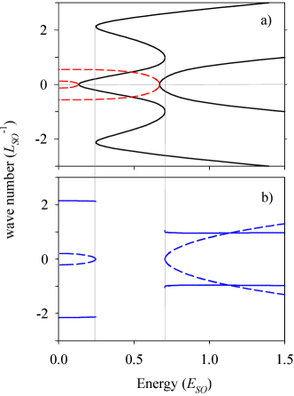
Figure 1: (Color online) Band structure as a function of energy for $\Delta_{B}=0.4E_{SO}$, $\Delta_{0}=0.25E_{SO}$, $\mu=0.1E_{SO}$, $\phi_{B}=\pi/4$. Solid and dashed lines correspond to $\Re(k)$ and $\Im(k)$, respectively. Panel a) shows modes having only one nonvanishing component of the wave number: solid lines are for propagating modes with $\Im(k)=0$ while dashed lines are for evanescent modes with $\Re(k)=0$. Panel b) shows the complex $k$’s for evanescent modes with both real and imaginary parts. The units are defined in Eqs. (9) and (10). Thin gray lines are guides helping the eye to correlate the position of the band extrema.

As an illustrative example, Fig. 1 shows a typical complex band structure. Notice that, contrary to common band representations, we choose the energy as horizontal axis since, within our approach, $E$ is given and the wave numbers are inferred. We only display the positive energy solutions, the negative ones corresponding to the specular image with respect to $E=0$. As in Ref. [ore11, ] we set our energy units using the Rashba interaction as a reference. Specifically, our length and energy units are

$$L_{SO} = \frac{\hbar^{2}}{\alpha m}\;,$$ (9)

$$E_{SO} = \frac{\alpha^{2}m}{\hbar^{2}}\;.$$ (10)

The propagating states in Fig. 1a agree with those already discussed in Refs. [ore11, ; kli12, ]. The evanescent states provide, however, a novel view. We distinguish two types of evanescent modes: those shown in Fig. 1a have a purely imaginary wave number, while those with wave numbers having both real and imaginary parts are shown in panel b). For a given energy, wave numbers always come in sets $\{k,k^{*},-k,-k^{*}\}$ or, equivalently, as $\pm|\Re(k)|\pm i|\Im(k)|$, where $\Re$ and $\Im$ stand for real and imaginary parts, respectively.ser07 That is, wave numbers come in quartets when both real and imaginary parts are non vanishing (panel b) and in pairs when the wave number is either purely real or purely imaginary (panel a).

Figure 1 shows that propagating and evanescent bands can be smoothly connected by the extrema points. In panel a) this connection is clearly seen as horizontal parabolas of opposite curvatures, showing how a purely imaginary wave number transforms into a purely real one as the energy increases. In panel b), $\Re(k)$ of an evanescent state connects with the extremum of the corresponding propagating band, while the imaginary part disappears when entering the propagating band sector. For a given energy, there are always 8 modes, as corresponds to a quadratic kinetic energy and the $4\times 4$ matrix in Eq. (II.1).

Summarizing this section, we stress that the suggested approach is a robust numerical algorithm allowing the determination of the complex band structure for an arbitrary set of parameters. We will focus next on the description of edge states, in particular zero energy ones representing Majorana modes.

II.2 Edge states

The complex band structure contains the necessary information on all possible eigenstates. In particular, localized states for which the wave function fades away of some defect or interface are, in general, superpositions of evanescent states. Let us consider a semi-infinite 1D system restricted to $x\geq 0$. A priori, we expect the abrupt edge at $x=0$ to allow the formation of localized states vanishing at $x=0$ and decaying towards $x\to\infty$. Such a state has to be a superposition of evanescent waves having $\Im(k)>0$. Let us assume that the set of such wave numbers is $\{\tilde{k}\}$, containing $\tilde{N}$ modes for a given energy $E$. The boundary condition an edge state has to fulfill is then

$$\sum_{k\in\{\tilde{k}\}}C_{k}\,\psi_{s_{\sigma}s_{\tau}}^{(k)}=0\;,$$ (11)

where the $C_{k}$’s are complex numbers and the $\psi_{s_{\sigma}s_{\tau}}^{(k)}$’s are the state amplitudes defined in the preceding subsection.

Equation (11) is a set of four linear equations, for $(s_{\sigma}s_{\tau})=(++,+-,-+,--)$, and $\tilde{N}$ unknown $C_{k}$’s. We can immediately conclude that if $\tilde{N}<4$ no edge state is possible since there are less unknowns than equations in Eq. (11). That is, if there are less than 4 evanescent modes with $\Im(k)>0$ only the trivial solution $C_{k}=0$ is possible, i.e., no physical solution is present. On the contrary, if $\tilde{N}>4$ it will always be possible to find a set of nonvanishing $C_{k}^{\prime}s$. If $\tilde{N}=4$ the nontrivial solution will be possible if the system matrix is singular (zero determinant). In that case the condition for the existence of an edge state is

$$\det\{\psi_{s_{\sigma}s_{\tau}}^{(k)}\}=0\;.$$ (12)

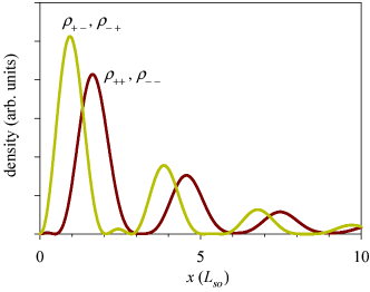
Figure 2: (Color online) Densities of the Majorana mode (edge state at zero energy) corresponding to the complex band structure of Fig. 1. The definition of $\rho_{s_{\sigma},s_{\tau}}(x)$ is given in Eq. (14).

For instance, in the case of Fig. 1 the requirement of at least 4 evanescent modes restricts the possibility of an edge mode to energies $E<0.1E_{SO}$. We have also computed the determinant of Eq. (12) finding that it vanishes only for $E=0$, while it grows linearly for $E>0$. Therefore, in this example a zero energy edge state is formed. This is a Majorana mode for which Fig. 2 displays the corresponding density profile, obtained as

$$\rho(x) \equiv \sum_{s_{\sigma}s_{\tau}}{\rho_{s_{\sigma}s_{\tau}}(x)}\;,$$ (13)

$$\rho_{s_{\sigma}s_{\tau}}(x) = \sum_{kk^{\prime}}{C_{k^{\prime}}^{*}C_{k}\,\psi^{(k^{\prime})*}_{s_{\sigma}s_{\tau}}\psi^{(k)}_{s_{\sigma}s_{\tau}}e^{i(k-{k^{\prime}}^{*})x}}\;.$$ (14)

As expected, the densities vanish at $x=0$ and decay with damped oscillations for increasing $x$. This behavior is in good agreement with previous results.kli12 Notice also that because of symmetry the densities remain invariant after spin-isospin inversion.

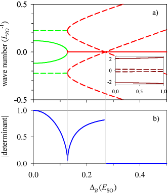
Figure 3: (Color online) a) Complex band structure as a function of $\Delta_{B}$ for fixed $E=0$, $\Delta_{0}=0.25E_{SO}$, $\mu=0.1E_{SO}$, $\phi_{B}=0$. As in Fig. 1, solid and dashed lines display real and imaginary parts of the wave number. The inset shows 4 modes with a large value of $\Re(k)$. b) Absolute value of the determinant Eq. (12). A vanishing determinant is the condition for the existence of an edge state.

The above results can be taken as examples of the method and its capabilities and we now address the question of how to rationalize the existence of topological phases. It was advanced by Oreg et al. ore11 that the signature of an emergent topological phase is the closing and reopening of the $k=0$ gap in the band structure of propagating states as one Hamiltonian parameter is varied. Increasing the Zeeman energy in a parallel field geometry the critical parameter for the topological transition is

$$\Delta_{B}^{(c)}=\sqrt{\Delta_{0}^{2}+\mu^{2}}\;,$$ (15)

such that zero-energy edge (Majorana) modes are present only when $\Delta_{B}>\Delta_{B}^{(c)}$. In the transverse field geometry, no zero energy modes are ever present. Let us analyze this scenario from the evanescent band structure point of view.

Figure 3 shows the evolution of the wave numbers at zero energy as a function of the Zeeman parameter. The field orientation is along $x$ and, in this case, we always find 8 evanescent modes for any $\Delta_{B}$. This means that there is no propagating mode for this energy. Notice that four evanescent modes with a rather structureless behavior and having a large real part of the wave number are shown in the inset. In panel b) we display the absolute value of the determinant Eq. (12) as a function of $\Delta_{B}$. The determinant has a discontinuous behavior: it decays from its maximal value for $\Delta_{B}=0$; it has an accidental zero for $\Delta_{B}\approx 0.13E_{SO}$, when all wave numbers in Fig. 3a become purely imaginary; and it consistently vanishes for $\Delta_{B}>0.27E_{SO}$, after the point where $\Im(k)$ vanishes for two of the modes.

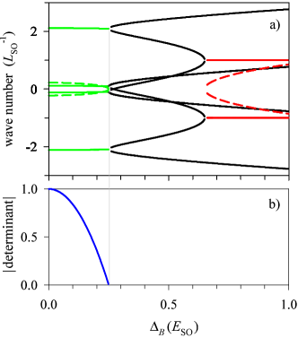
Figure 4: (Color online) Same as Fig. 3 for field orientation along $y$ ($\phi_{B}=\pi/2$). In panel b) the determinant can only be defined for $\Delta_{B}<0.25E_{SO}$, when there are 4 evanescent modes with $\Im(k)>0$.

The results in Fig. 3 show that Majorana modes exist above a critical field ($0.27E_{SO}$ in that case) which is in agreement with the $\Delta_{B}^{(c)}$ of Eq. (15) anticipated by Oreg and collaborators.ore11 Not only this, the analysis in terms of evanescent modes also sheds light on the reason why the topological transition is signaled by the vanishing of a gap for propagating states. Indeed, when $\Delta_{B}=\Delta_{B}^{(c)}$ in Fig. (3) the complete vanishing of $k$ for two of the modes indicates that they loose the evanescent character and become propagating, but only for a single point in $\Delta_{B}$ and thus they are not seen in panel a) as fully developed bands. At this value of $\Delta_{B}$, therefore, there is no energy gap for propagating states. Notice, finally, that Fig. 3 also shows that the vanishing of the gap for propagating states occurs for a wave number $k=0$.

When the field is in transverse direction ($y$), as in Fig. 4, no Majorana modes are present. Quite remarkably, in this case there are propagating modes at zero energy (dark solid lines appearing for $\Delta_{B}>0.25E_{SO}$). The condition of at least four evanescent modes with $\Im(k)>0$ is fulfilled only when $\Delta_{B}<0.25E_{SO}$ but, even in this region, no edge state is allowed because of the non vanishing determinant, as shown in panel b).

III The 2D case

We consider now the generalization of the complex band structure approach to include one extra spatial degree of freedom in the transverse direction to the wire. As before, we assume the wire to be infinite along $x$, but now motion along $y$ is also possible with the restriction $-L_{y}/2\leq y\leq L_{y}/2$. This corresponds to a hard wall confinement in $y$ within a square well of length $L_{y}$. We call this a 2D case although in the literature the name quasi-1D is often used to emphasize that there is confinement in the transverse direction while along the longitudinal one motion is free.

III.1 Hamiltonian

The generalization of Hamiltonian (1) is

$${\cal H}_{2D} = \left(\frac{p_{x}^{2}}{2m}+\frac{p_{y}^{2}}{2m}+V(y)-\mu\right)\tau_{z}+\Delta_{B}\vec{\sigma}\cdot\hat{n}$$ (16)

$$+ \Delta_{0}\tau_{x}+\frac{\alpha}{\hbar}\left(p_{x}\sigma_{y}-p_{y}\sigma_{x}\right)\tau_{z}\;,$$

where $V(y)$ is the square well of length $L_{y}$ mentioned above. Besides $y$ confinement Hamiltonian (16) includes the transverse kinetic energy and a $p_{y}$-dependent Rashba term that, following a usual convention, we call the Rashba mixing term. The mixing character of this term can be understood from the fact that the $p_{y}$ operator couples different square well eigenstates.

The analysis proceeds in a similar way to the preceding 1D case with the important difference that now the state amplitudes of Eq. (3) become functions of $y$,

$$\psi_{s_{\sigma}s_{\tau}}\to\psi_{s_{\sigma}s_{\tau}}(y)\;.$$ (17)

Accordingly, the algebraic Eq. (II.1) becomes a second order differential equation due to the dependence on $p_{y}^{2}$ and $p_{y}$

$$\left[\rule{0.0pt}{17.07182pt}\left(\frac{p_{y}^{2}}{2m}+\displaystyle\frac{\hbar^{2}k^{2}}{2m}-\mu\right)s_{\tau}+\Delta_{B}s_{\sigma}+\alpha ks_{\sigma}s_{\tau}\sin\phi_{B}\right.$$

$$\hskip 28.45274pt\left.\rule{0.0pt}{17.07182pt}-E\right]\psi_{s_{\sigma}s_{\tau}}(y)+\Delta_{0}\,\psi_{s_{\sigma}\overline{s_{\tau}}}(y)$$

$$+\alpha s_{\tau}\left(ik\,s_{\sigma}\cos\phi_{B}\,-\frac{p_{y}}{\hbar}\right)\psi_{\overline{s_{\sigma}}s_{\tau}}(y)=0\;.$$ (18)

Another difference with respect to the 1D case is the dependence on the magnetic field orientation. Now $x$ and $z$ orientations are no longer physically equivalent due to the orbital currents present in the latter. However, in Eq. (III.1) we have again assumed a magnetic field in the $xy$ plane with an azimuthal angle $\phi_{B}$ since, in this geometry, there are no orbital effects of the field.

From the numerical point of view solving Eqs. (III.1) for an arbitrary $k$ is much more demanding than the 1D case. We have devised a practical algorithm,ser07 introducing a uniform grid in $y$ and an arbitrary matching point $y_{m}$. The differential equation (III.1) on all grid points but $y_{m}$ is rewritten using finite difference formulas, with an important caveat: crossing from left to right of the matching point is avoided using non centered finite difference formulas. Another condition is that the state amplitude vanishes at the edges of the $y$ domain. At the matching point $y_{m}$, instead of Eq. (III.1), we require the conditions

$$\begin{array}[]{rcll}\psi_{s_{\sigma}s_{\tau}}(y_{m})&=&1\;,&{\rm if}\;(s_{\sigma},s_{\tau})=(s,t)\,,\\ \left(\frac{d^{(L)}}{dy}-\frac{d^{(R)}}{dy}\right)\psi_{s_{\sigma}s_{\tau}}(y_{m})&=&0\;,&{\rm if}\;(s_{\sigma},s_{\tau})\neq(s,t)\,,\end{array}$$ (19)

where $(s,t)$ are a pair of arbitrarily chosen spin and isospin labels. In Eq. (19) we have used the notation $d^{(L,R)}/dy$ to indicate derivatives at $y_{m}$ using only left ($L$) or right (R) neighboring grid points. Of course, a physically valid wave number must correspond to a continuous first derivative of $\psi_{st}(y)$ at the matching point. We thus numerically determine $k$ from the zeros of the function

$${\cal F}_{2D}(k)=\left|\left(\frac{d^{(L)}}{dy}-\frac{d^{(R)}}{dy}\right)\psi_{st}(y_{m})\right|^{2}\;.$$ (20)

As in the 1D case, when ${\cal F}_{2D}(k)=0$ is fulfilled the solution from Eq. (19) is equivalent to that of the full Eq. (III.1).

The robustness of the suggested numerical algorithms, both for 2D and 1D, is seen in the fact that for any complex $k$ the ${\cal F}$ functions can be computed, avoiding singular matrices or ill-behaved numerical problems.tom02 Finding the physically allowed $k$’s is then accomplished scanning the complex $k$ plane to determine the zeros of ${\cal F}$ with the desired accuracy. We have checked that the solution is not affected by the arbitrary choice of state components $(s,t)$ and matching point $y_{m}$. Besides, since Eq. (III.1) involves only one variable ($y$), high numerical precission can be easily obtained using large enough numbers of grid points ($N_{y}\approx 500$) and of points for the finite difference derivatives (5 to 11 points).

III.2 2D edge states

In 2D the boundary condition for an edge state with $x\geq 0$ is similar to Eq. (11), with the state amplitudes changed from scalars to $y$-functions,

$$\sum_{k\in\{\tilde{k}\}}C_{k}\,\psi_{s_{\sigma}s_{\tau}}^{(k)}(y)=0\;.$$ (21)

We immediately notice that now the boundary condition requires an infinite number of evanescent states $\{\tilde{k}\}$ due to the infinite number of possible values of $y$. In practice, a truncation to a restricted set of $\tilde{N}$ evanescent modes has to be done and, accordingly, the condition (21) can be imposed on $\tilde{N}/4$ values of $y$ (the number of modes should be a multiple of 4).

Instead of using specific values of $y$ in Eq. (21), we have projected Eq. (21) on the set of $\tilde{N}$ evanescent modes, finding the matrix equation

$$\sum_{k\in\{\tilde{k}\}}{\cal M}_{k^{\prime}k}\,C_{k}=0\;,$$ (22)

where

$${\cal M}_{k^{\prime}k}=\sum_{s_{\sigma}s_{\tau}}\int{dy\,\psi_{s_{\sigma}s_{\tau}}^{(k^{\prime})*}(y)\,\psi_{s_{\sigma}s_{\tau}}^{(k)}(y)\,\;.}$$ (23)

When the number $\tilde{N}$ of evanescent modes is large enough, the zero eigenvalues of matrix ${\cal M}$ correspond to Majorana edge states. This Hermitian matrix can be diagonalized numerically with standard methods. For the 1D case of the preceding section the diagonalization of matrix ${\cal M}$ is equivalent to the approach based on the determinant, Eq. (12), since a zero eigenvalue is associated with a vanishing determinant. In 2D matrix ${\cal M}$ allows a truncation of the infinite number of evanescent modes.

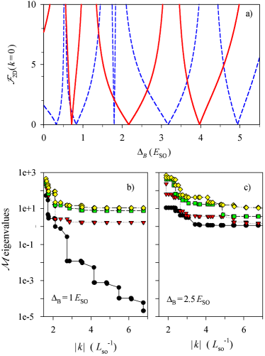
Figure 5: (Color online) a) Value of the derivative discontinuity ${\cal F}_{2D}$ for $k=0$. Solid and dashed lines correspond to presence and absence of the Rashba mixing term, respectively. In absence of Rashba mixing (dashes), the nodes signal the appearance of successive Majorana modes when increasing $\Delta_{B}$. For the case with Rashba mixing, panels b) and c) show the evolution of the lower eigenvalues of matrix ${\cal M}$ when increasing the number of evanescent modes. The appearance of a zero eigenvalue is seen in b). Parameters: $\Delta_{0}=0.25E_{SO}$, $\mu=0$, $E=0$, $L_{y}=5L_{SO}$.

The complete determination of the evanescent bands in 2D is a very tedious task due to the large number of states when varying $\Delta_{B}$. Instead of finding the equivalent to Fig. 3 for the 2D case, we have followed a different approach to determine the existence of Majorana edge states. Since the topological phase transition is signaled by a complete vanishing of the complex wave number, we have scanned the value of ${\cal F}_{2D}(k=0)$ when varying the Zeeman parameter $\Delta_{B}$ of the Hamiltonian. The regions between nodes of ${\cal F}_{2D}(k=0)$ are the different phases, and we have just studied a few selected values of $\Delta_{B}$ in each region. For a given $\Delta_{B}$, we look for a set of evanescent modes in the complex-$k$ plane. With these modes we then find matrix ${\cal M}_{k^{\prime}k}$ and compute its lower eigenvalues. As discussed above, each vanishing eigenvalue is associated with a Majorana zero mode.

In absence of Rashba mixing each transverse mode of the quantum wire behaves as an independent 1D system: there is an onset for the appearance of the $n$-th band Majorana mode

$$\Delta_{B,n}^{(c)}=\sqrt{\Delta_{0}^{2}+(\mu-\varepsilon_{n})^{2}}\;,$$ (24)

where $\varepsilon_{n}$ is the $n$-th eigenvalue of the transverse quantum well, and multiple Majorana modes are possible independently. This physics is contained in the results shown as a dashed line in Fig. 5a where, as could be expected, the derivative discontinuity ${\cal F}_{2D}(k=0)$ has nodes precisely when $\Delta_{B}=\Delta^{(c)}_{B,n}$. We have also obtained that, in this case, matrix ${\cal M}$ has $n$ different zero eigenvalues when evaluated for a value of $\Delta_{B}$ such that $\Delta^{(c)}_{B,n}<\Delta_{B}<\Delta^{(c)}_{B,n+1}$. In practice, a fast numerical convergence of these lower eigenvalues to $\approx 10^{-9}$ is easily obtained.

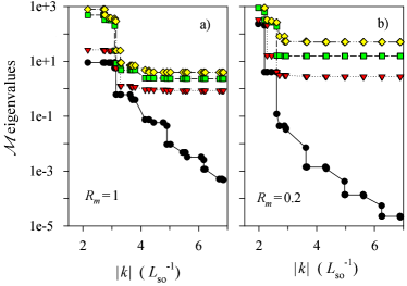
Figure 6: (Color online) Convergence of the lower eigenvalues of matrix ${\cal M}$ when $\Delta_{B}$ lies between the third and fourth nodes of ${\cal F}_{2D}(k=0)$. Left panel corresponds to full Rashba mixing ($R_{m}=1$) with $\Delta_{B}=4.5E_{SO}$ (cf. Fig. 5a) while right panel is for an artificially reduced mixing ($R_{m}=0.2$) with $\Delta_{B}=2.5E_{SO}$. The remaining parameters are the same of Fig. 5.

Conspicuous modifications to the above scenario are seen when including the Rashba mixing. Notice that in Fig. 5 we are assuming a regime of strong spin-orbit in which $E_{SO}\approx\varepsilon_{n+1}-\varepsilon_{n}$. We find that for $\Delta_{B}<0.71E_{SO}$, below the first node of Fig. 5a solid line, the matrix ${\cal M}$ has no zero eigenvalue. In the region between the first and second nodes, $0.71E_{SO}<\Delta_{B}<2.17E_{SO}$, we find clear evidence of a zero eigenvalue, as proved in Fig. 5b. Convergence is, however, rather slow and a large number of evanescent states is required. As a practical scheme, we have included the evanescent states in an ordered way, taking the modulus of the complex wave number as ordering parameter. This criterion gives, for instance, that in Fig. 5b for $|k|<7L_{SO}^{-1}$ we include a total of 44 evanescent modes.

In the region $2.17E_{SO}<\Delta_{B}<3.97E_{SO}$, between the second and third nodes of Fig. 5a solid line, the lower eigenvalues of matrix ${\cal M}$ converge to finite values, as shown in Fig. 5c for $\Delta_{B}=2.5E_{SO}$. This behavior is due to the Rashba mixing, for, in its absence, we find two zero eigenvalues in this region. Though numerical, the difference between panels b) and c) of Fig. 5 is quite clear and leads to the conclusion that Rashba mixing hinders the coexistence of two Majorana modes, which is in agreement with the results of Ref. [lim12, ] for finite systems. It is remarkable that this hindrance persists even in the semi-infinite system.

We focus next on the existence of edge states when $\Delta_{B}$ lies between the third and fourth nodes of ${\cal F}_{2D}(k=0)$; that is, when three zero modes are present without Rashba mixing. As shown in Fig. 6a, one Majorana mode again emerges when enough evanescent states are included in matrix ${\cal M}$. This result agrees with the physical scenario found in Ref. pot10, using a tight-binding approach; i.e., just a single zero mode is protected in non trivial topological phases. For the sake of discussion, we have artificially weighted the Rashba mixing term by a factor $R_{m}$ in Fig. 6. Convergence with the $|k|$ cutoff is much slower with full mixing ($R_{m}=1$) than with a reduced one ($R_{m}=0.2$), clearly indicating the relevance of this mechanism.

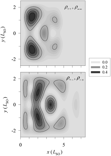
Figure 7: Density distributions for the Majorana zero mode shown in Fig. 5b. Arbitrary units are used in a gray color scale. Contour lines are displayed for a better presentation.

For completeness, Fig. 7 shows the density distributions corresponding to the Majorana mode of Fig. 5b, using a 2D generalization of Eq. (14). Notice that, on the scale of the figure, the density vanishes for $x=0$ and all values of $y$ which is indicating the good convergence of the boundary condition with the number of evanescent modes. Of course, the densities also vanish asymptotically for $x\to\infty$ and, as in the 1D case, remain invariant when inverting spin and isospin.

IV Conclusions

We have discussed the physics of Majorana modes in semi-infinite 1D and 2D wires using the complex band structure approach. This formalism provides a natural description of the zero-energy edge modes as superpositions of multiple evanescent waves. The boundary condition of a vanishing wave function at the edge cannot always be fulfilled, this limitation defining the parameter regions (phases) where Majorana modes exist.

The phase transition occurs when for zero energy the complex wave number of an evanescent band vanishes. The phase transition is seen as the emergence of a zero eigenvalue of matrix ${\cal M}$, defined in Eq. (23). In 1D the analysis with matrix ${\cal M}$ is equivalent to the determinant of state amplitudes; while in 2D matrix ${\cal M}$ allows to monitor the convergence of the lower eigenvalues when the number of evanescent modes is increased. In 2D we find evidence that, in case of a strong Rashba coupling, the Rashba mixing effect hinders the coexistence of multiple Majorana modes in the semi-infinite wire. In agreement with tight-binding models,pot10 alternating regions having zero and one Majorana modes are found when increasing $\Delta_{B}$.

- (1) For recent reviews, see J. Alicea, Rep. Prog. Phys. 75, 076501 (2012); X. L. Qi and S. C: Zhang, Rev. Mod. Phys. 83, 1057 (2011).
- (2) L. Fu and C. L. Kane, Phys. Rev. Lett. 100, 096407 (2008).
- (3) A. R. Akhmerov, J. Nilsson, and C. W. J. Beenakker, Phys. Rev. Lett. 102, 216404 (2009).
- (4) Y. Tanaka, T. Yokoyama, and N. Nagaosa, Phys. Rev. Lett. 103, 107002 (2009).
- (5) K. T. Law, P. A. Lee, and T. K. Ng, Phys. Rev. Lett. 103, 237001 (2009).
- (6) R. M. Lutchyn, J. D. Sau, and S. Das Sarma, Phys. Rev. Lett. 105, 077001 (2010).
- (7) Y. Oreg, G. Refael, and F. von Oppen, Phys. Rev. Lett. 105, 177002 (2010).
- (8) K. Flensberg, Phys. Rev. B 82, 180516 (2010).
- (9) A. C. Potter and P. A. Lee, Phys. Rev. Lett. 105, 227003 (2010); Phys. Rev. B 83, 094525 (2011).
- (10) A. R. Akhmerov, J. P. Dahlhaus, F. Hassler, M. Wimmer, and C. W. J. Beenakker, Phys. Rev. Lett. 106 057001 (2011).
- (11) S. Gangadharaiah, B. Braunecker, P. Simon, and D. Loss, Phys. Rev. Lett. 107, 036801 (2011).
- (12) R. Egger, A. Zazunov, and A. L. Yeyati, Phys. Rev. Lett. 105, 136403 (2010).
- (13) R. M. Lutchyn, T. D. Stanescu, and S. Das Sarma, Phys. Rev. Lett. 106, 127001 (2011).
- (14) T. D. Stanescu, R. M. Lutchyn, and S. Das Sarma, Phys. Rev. B 84, 144522 (2011).
- (15) A. Zazunov, A. L. Yeyati, and R. Egger, Phys. Rev. B 84, 165440 (2011)
- (16) M. Wimmer, A. R. Akhmerov, J. P. Dahlhaus, C. W. J. Beenakker, New Journal of Physics 13 053016 (2011).
- (17) R. Zitko and P. Simon, Phys. Rev. B 84, 195310 (2011).
- (18) A. Golub, I. Kuzmenko, Y. Avishai, Phys. Rev. Lett. 107, 176802 (2011).
- (19) J. Li, G. Fleury, M. Büttiker, Phys. Rev. B 85, 125440 (2012).
- (20) J. Klinovaja, S. Gangadharaiah, and D. Loss, Phys. Rev. Lett. 108, 196804 (2012).
- (21) J. Klinovaja and D. Loss, Phys. Rev. B 86, 085408 (2012).
- (22) C. W. J. Beenakker, arXiv:1112.1950.
- (23) V. Mourik, K. Zuo, S. M. Frolov, S. R. Plissard, E. P. A. M. Bakkers, and L. P. Kouwenhoven, Science 336, 1003 (2012).
- (24) M. T. Deng, C. L. Yu, G. Y. Huang, M. Larsson, P. Caroff, Nano Lett. 12, 6414 (2012).
- (25) L. P. Rokhinson, X. Liu, and J. K. Furdyna, Nature Physics 8, 795 (2012).
- (26) A. Das, Y. Ronen, Y. Most, Y. Oreg, M. Heiblum, H. Shtrikman, Nature Physics 8, 887 (2012).
- (27) S. Sasaki, M. Kriener, K. Segawa, K. Yada, Y. Tanaka, M. Sato, and Y. Ando, Phys. Rev. Lett. 107, 217001 (2011).
- (28) J. R. Williams, A. J. Bestwick, P. Gallagher, S. S. Hong, Y. Cui, A. S. Bleich, J. G. Analytis, I. R. Fisher, and D. Goldhaber-Gordon, Phys. Rev. Lett. 109, 056803 (2012).
- (29) A. M. Lobos, R. M. Lutchyn, and S. Das Sarma, Phys. Rev. Lett. 109, 146403 (2012).
- (30) S. Tewari, T. D. Stanescu, J. D. Sau, and S. Das Sarma, Phys. Rev. B 86, 024504 (2012).
- (31) J. S. Lim, L. Serra, R. López, and R. Aguado, Phys. Rev. B 86, 121103 (2012).
- (32) J. S. Lim, R. López, and L. Serra, New Journal of Physics 14, 083020 (2012).
- (33) D. I. Pikulin, J. P. Dalhaus, M. Wimmer, S. Schomerus, and C. W. J. Beenakker, New Journal of Physics 14, 125011 (2012).
- (34) A. M. Cook, M. M. Vazifeh, and M. Franz, Phys. Rev. B 86, 155431 (2012).
- (35) D. Rainis, L. Trifunovic, J. Klinovaja, and D. Loss, Phys. Rev. B 87, 024515 (2013).
- (36) W. Shockley, Phys. Rev. 56, 317 (1939).
- (37) J. K. Tomfohr and O. F. Sankey, Phys. Rev. B 65, 245105 (2002).
- (38) L. Serra, D. Sánchez and R. López, Phys. Rev. B 76, 045339 (2007).
- (39) In 1D the analytic form of the Hamiltonian energy eigenvalue as a function of is known (see, e.g., Ref. [ore11, ]). Therefore, determining the allowed ’s amounts to finding the (complex) roots of an eigth degree polynomial in this case. However, the extension to 2D of this approach is, at the very least, unclear since the analytic eigenvalues are unknown in 2D.