Abstract

In this paper we outline some mathematical questions that emerge from trying to “turn the scientific method into math”. Specifically, we consider the problem of experiment planning (choosing the best experiment to do next) in explicit probabilistic and information theoretic terms. We formulate this as an information measurement problem; that is, we seek a rigorous definition of an information metric to measure the likely information yield of an experiment, such that maximizing the information metric will indeed reliably choose the best experiment to perform. We present the surprising result that defining the metric purely in terms of prediction power on observable variables yields a metric that can converge to the classical mutual information $I(X;\Omega)$ measuring how informative the experimental observation $X$ is about an underlying hidden variable $\Omega$. We show how the expectation potential information metric can compute the “information rate” of an experiment as well its total possible yield, and the information value of experimental controls. To illustrate the utility of these concepts for guiding fundamental scientific inquiry, we present an extensive case study (RoboMendel) applying these metrics to propose sequences of experiments for discovering the basic principles of genetics.

1 Introduction

1.1 The RoboMendel Problem

We first outline an intuitive introduction to our example application problem and its assumptions. We consider the problem of a robot scientist (whom we call “RoboMendel”) assigned the task of improving his theory of inheritance of traits, as measured by his ability to predict the outcome of any possible cross between animals, plants and other living creatures. We will derive precise definitions (e.g. of this “prediction power” metric) later; for the moment we focus on an intuitive statement of the problem and its goal. We assume that RoboMendel begins roughly where Mendel began, namely:

• He starts with a simple “like father, like son” (LFLS) model of inheritance that treats heritable variation as a set of distinct clusters (i.e. species) in “trait space”. That is, each species has a distinct distribution of trait values, and all members of that species are drawn i.i.d. (independent and identically distributed) from that multi-dimensional distribution. Members of a species can only give birth to new instances of the same species (again drawn i.i.d. from its trait distribution). The simplest version of this model asserts that two parents (mother and father) are required to give progeny, and that they must be from the same species.

• Beyond this, RoboMendel does not know any modern biology or technology, and thus can only detect visible, macroscopic trait differences that Mendel could see with his eyes.

• Concretely, the set of all possible “inheritance” experiments RoboMendel could do is simply the set of all possible crosses between different creatures. For example, he could try to cross a mouse with a lion, or a pea plant with another pea plant, etc.

• We define RoboMendel’s goal as elucidating predictive laws of inheritance, which we define as traits that in any individual depend on the traits of its ancestors (as opposed to other factors such as the weather). For example, we can easily see that the “like father, like son” model fits this definition, as follows. For each individual organism $i$, we associate with it a trait vector $\vec{X}_{i}$ of its observed trait values, and a hidden value $\Theta_{i}$ indicating what species it belongs to. Mathematically, the problem of predicting an individual’s traits ($p(\vec{X}_{i}|\Theta_{i})$) and the converse problem of inferring its species ($p(\Theta_{i}|\vec{X}_{i})$) are linked by Bayes’ Law. The main assertion of LFLS, namely that $\Theta_{\text{child}}=\Theta_{\text{dad}}=\Theta_{\text{mom}}$, indeed makes the parental traits $\vec{X}_{\text{dad}},\vec{X}_{\text{mom}}$ the sufficient statistics for predicting the child’s traits $\vec{X}_{\text{child}}$, so LFLS fits our definition of a “predictive law of inheritance”. We will later define precisely how this statement of a “target problem” is translated into an information metric.

• RoboMendel is initially shown the same observation that Mendel initially saw, namely that whereas pea plants normally have purple flowers, one year he finds a pea plant (ostensibly from last year’s purple-flowered parents) with white flowers. We will refer to this trait as Wh, and the original (purple- flowered) trait as Pu.

• RoboMendel simply seeks to choose the best possible experiment to do next (mouse X lion? pea X pea? etc.), performs the experiment, observes the results, and again chooses the best experiment to do next, and so on, cycle after cycle. By “best” we simply mean the most efficient path for improving its prediction power for trait inheritance in general.

• We seek a single, general principle for optimizing this process, in the form of a measure of the likely information yield of an experiment, expressed in terms of how much it could increase RoboMendel’s prediction power. That is, we seek a single metric that answers all of the above questions, ranging from fine details of experiment design optimization (e.g. how many replicates of this observation should I collect? Can I terminate this experiment now based on the results I’ve obtained so far?) to big decisions about what phenomena to study (e.g. should we study mouse X lion, or pea plant flower color variation?). Specifically, we mean that it should choose the experimental design that maximizes this information metric (typically expressed in terms of information yield per cost, assuming that both “setup costs” and “per observation costs” are properly accounted for).

1.2 Initial Parameters

The RoboMendel problem begins with the observation of one pea plant with white flowers, apparently descended from regular purple-flowered parents (since all pea plants previously encountered by RoboMendel had purple flowers). We first enumerate the basic probability factors that frame his experiment planning process:

• p(LFLS): this represents our confidence in our current like-father-like-son model of genetics. Note that this reflects both repeated observations that fit the model (i.e. each time we actually observe an animal or plant born from its parent, we see that it looks like the same species as its parent(s)), and an implicit absence of observations that violate the model (e.g. we never see evidence of successful inter-species crosses, like a zebra with a long neck like a giraffe). Assuming that we have observed on the order of 1000 species, we might set this probability at p(LFLS) = 0.999.

• p(Wh-heritable): this estimates the probability that Wh is actually a heritable trait. Note that if Wh is not a heritable trait (for example, it might be caused by an environmental factor), then experiments studying it will have zero information value for our targeted metric, which focuses specifically on genetic inheritance. In the absence of any previous data on this trait, we assume an uninformative prior p(Wh-heritable) = 0.5.

• p(same-species): this estimates the probability that Wh is a member of the same species as Pu, the regular purple- flowered pea plant. Note that same-species does not assume Wh-heritable; they are two separate hypotheses. Again we assume an uninformative prior p(same-species) = 0.5. Intuitively, on the one hand our prior belief was that it was descended from Pu parents, but on the other hand it doesn’t look like them.

Note that if both Wh-heritable and same-species are true, this would strongly contradict LFLS.

2 Foundations of the Experiment Planning Information Metric

In this section we outline a general information metric for experiment planning. This metric is based on standard concepts in statistical inference and information theory [1] [2] [3] [4] ; our interest here is how they apply to the specific problems of experiment planning and the scientific method.

2.1 Empirical Information

2.1.1 Defining “Prediction Power”

We have previously defined “empirical information” estimators based on two principles: measuring a model’s prediction power strictly for observable variables (rather than inferring hidden variables); estimating this metric from a random sample of observations, with a Law of Large Numbers (LLN) guarantee of convergence to a classic information metric such as relative entropy or mutual information [4] . Here we briefly outline their application to experiment planning. We define the relative information value of a model in terms of its increase in prediction power of one likelihood model $\Psi(X)$ relative to another $\Psi_{0}(X)$, as the difference in the expectation log-likelihoods of the observable $X$ under the two models

$$\Delta I=E_{\Omega}(\log{\Psi(X)})-E_{\Omega}(\log{\Psi_{0}(X)})$$

where the expectation is taken under the true (but unknown) distribution of the observable, $\Omega(X)$. Although this cannot be computed directly (because $\Omega(X)$ is unknown), it can be estimated empirically with a LLN convergence

$$\overline{L_{e}(\Psi)}=\frac{1}{n}\sum_{i=1}^{n}{\log{\Psi(X_{i})}}\to E_{\Omega}(\log{\Psi(X)})$$

as the sample size $n\to\infty$; we refer to $\overline{L_{e}(\Psi)}$ as the empirical log-likelihood. We then define the empirical information $\overline{I_{e}(\Psi)}$ as the estimated increase in prediction power relative to the marginal distribution of the observable, $p(X)$:

$$\overline{I_{e}(\Psi)}=\overline{L_{e}(\Psi)}-\overline{L_{e}(p)}$$

Note that this is a pure likelihood metric (i.e. no consideration of the prior probability of model $\Psi$), similar to the classical likelihood metrics used for Maximum Likelihood (ML), the Akaike Information Criterion (AIC) [5] , Bayesian Information Criterion (BIC) [6] , and various log-likelihood ratio tests. One difference should be emphasized: LLN convergence requires that $I_{e}(\Psi)$ be measured on data $X_{i}$ that are conditionally independent of the model $\Psi$ given the true distribution $\Omega$, i.e. on test data rather than training data, in marked contrast with ML, AIC, BIC and many other metrics designed for model-selection (i.e. choosing a model by maximizing the metric).

Example: after RoboMendel observes white flowers on some of his pea plants, he can try to improve the prediction power of his current model (which predicts that pea plants have only purple flowers) by adjusting it to predict that a certain fraction of pea flowers are white (Fig. 1C). He can then measure the empirical information gain of the new model on a set of observations of additional flowers. This validates that the new model greatly improves prediction power relative to the old model. Note however that it does not assess whether the new model truly fits the observations; we address this below with the potential information metric.

2.1.2 A Zero Information Principle

It is useful to highlight a simple but important feature of the metric: since information is defined as increased prediction power, any step that does not alter the prediction (i.e. $\Psi=\Psi_{0}$) must have zero information value.

This simple idea implies an interesting conundrum. Consider any new theory $\Psi^{\prime}$ proposed in response to observations that “do not fit” the existing model $\Psi_{0}$. Replacing the existing model with the new theory produces positive information (since the new theory fits the observations better). Now consider an experimental test of further predictions that the new model makes. If we were to perform that experiment and obtain results that do not fit the model $\Psi^{\prime}$, this would presumably have information value (again, because it would force us to change our predictive model). If on the other hand we obtained results that fit the model $\Psi^{\prime}$, that would appear to have zero information value (because no change in our predictions would result). On this basis, any kind of boolean rule for choosing our “current model” (i.e. the “weight” assigned to $\Psi^{\prime}$ must be either 0 or 1) would appear to lead to the following paradox. If we assign $\Psi^{\prime}$ a weight of 1, then the initial “proposal” step produces positive information, but the expectation information yield from the experiment to test it would be zero (because the boolean rule assigned zero probability to the negative result, and the positive result produces zero information yield). On the other hand if we assign it a weight of zero, then both the “proposal” and “test” steps would produce zero information. This suggests that only a “fuzzy rule” that allows it to be assigned a weight between 0 and 1 can ascribe positive information value both to proposing a new model and testing its predictions experimentally.

2.2 Expectation Information and the Hidden Mixture Problem

How does this principle affect our modeling of observables? First of all, it introduces a subtle change in the joint probability of multiple observations. For example, say RoboMendel observes a series of flowers from a randomly chosen individual. If the individual is drawn from a homogeneous population (under the LFLS model, from a single species) then these flower observations are “independent and identically distributed” (i.i.d.). However, if the individual is drawn from a hidden mixture of different species (e.g. one species with white flowers and one species with yellow flowers), then the flower observations are no longer independent; for example, if the first flower observed is yellow, that greatly increases the probability that subsequent flowers will be yellow. Note that the “fuzzy rule” principle of introducing a new model with a fractional weight implies exactly this kind of hidden mixture and consequent lack of independence.

2.2.1 The i.i.d. vs de Finetti Exchangeability Problem

This statistical distinction may at first seem subtle, but has fundamental importance, and deserves clear definition. Random variables $X_{1},X_{2},...$ are said to be “independent and identically distributed” (i.i.d.) if their joint distribution can simply be factored into a product of identical terms $p(X_{1},X_{2},...)=\prod_{i}{f(X_{i})}$ where the same marginal probability distribution $f()$ applies to each of the random variables. By contrast, random variables $X_{1},X_{2},...$ are said to be “exchangeable” if for any length $n$ and index sequences $i_{1},i_{2},...i_{n}$ and $j_{1},j_{2},...j_{n}$ (where each $i$ value is unique, and each $j$ value is unique), the joint probability distributions of the indexed variable sequences are identical: $p(X_{i_{1}},X_{i_{2}},...X_{i_{n}})=p(X_{j_{1}},X_{j_{2}},...X_{j_{n}})$ [7] . Clearly, if $X_{1},X_{2},...$ are i.i.d., then they are also exchangeable, but the converse is not true. Consider the case where the joint probability is

$$p(X_{1},X_{2},...)=\sum_{\Omega}{p(\Omega)\prod_{i}{\Omega(X_{i})}}$$

where the hidden variable $\Omega$ is allowed two or more possible values $\omega_{1},\omega_{2},...$. This expression is completely invariant with respect to exchange of different $X_{i},X_{j}$, so the random variables are exchangeable. However, they are not independent; instead they are conditionally independent given $\Omega$.

This definition is associated with the mathematician de Finetti, who proved that any infinite sequence of exchangeable Bernoulli variables is equivalent to a mixture of multiple i.i.d. Bernoulli sequences of the form given by the equation above [7] . In statistics, this definition occasions some subtle distinctions; that is, out of the many “standard results” that assume i.i.d. random variables, some of them extend without difficulty to the case where the random variables are exchangeable, while others do not.

De Finetti exchangeability is fundamental to the scientific method because science faces precisely this problem of an unknown mixture of hidden distributions. Canonical descriptions of the scientific method tend to gloss over this mixture problem, in that they discuss hypothesis testing as if the hypotheses were either “true” or “false”, i.e. true every single time we test them or false every single time we test them. This may seem like a natural attitude if one assumes that science only studies “eternal laws” i.e. hypotheses that by definition must be always true or always false in any given universe. But a priori, it is invalid to assume that because a hypothesis (“flowers are yellow”) tested true in one experiment, that it will therefore test true in all experiments.

Instead, we assert this should be treated as an empirical question. Specifically, we only assume the general model of a de Finetti mixture, and then use multiple observations to infer the weight parameters of the de Finetti mixture. This corresponds to replacing a boolean rule for choosing our current model, with a mixture model that combines multiple models with probabilities between zero and one. Of course, if multiple experiments in a variety of independent cases all confirm a given hypothesis, its mixture weight will converge to 1. As we shall show below, it is precisely this combination of initial uncertainty about the mixture followed by gradual convergence to an unchanging mixture, that drives the experiment planning process by predicting large expectation information yields for “new questions” vs. small information yields for “old questions” that have already been tested to convergence.

2.2.2 Expectation Empirical Information

This suggests an obvious extension of the empirical information concept. Empirical information represents a measure of our ability to predict various observables in a collection of scenarios that we have actually sampled. From the point of view of the de Finetti mixture, this metric is incomplete, in that it considers only scenarios we’ve already sampled, as opposed to the probable mix of familiar plus novel scenarios that an unbiased estimator should be based on. Conceptually, we formulate this as an expectation value for the prediction power, taken over our posterior estimate of the de Finetti mixture. Intuitively, the value of this metric arises from two sources. First, truly general models have extrapolation power; that is, they extrapolate successfully to regions of observation space that were not actually sampled in the training process. Second, the de Finetti mixture estimation process can convince us through repeated testing that a model actually has such extrapolation power; that is, its prediction power for novel cases has been found to be consistently the same as for the original cases.

Example: RoboMendel’s LFLS model predicts what progeny will look like from any pair of parents, and repeated confirmations of its predictions increase RoboMendel’s posterior estimate of the fraction of cases that it applies to in the real world, converging to 100%.

2.2.3 Universal vs. Targeted Information Metrics

We can either define this metric across all possible observables, or for a targeted set of types of observable outcomes that we particularly care about. A universal information metric treats all observables as “equally valuable”; that is, 1 bit of improved prediction power for one observable (e.g. flower color) counts exactly the same in the metric as 1 bit of improved prediction power for any other observable (e.g. identifying the tumor type of a patient’s cancer biopsy). By contrast, a targeted metric specifies a particular set of observables that we wish to be able to predict as accurately as possible. For example, for the RoboMendel problem, we restrict the information metric specifically to predicting traits that actually depend on parental traits (i.e. they are genetic, not due to some other, environmental factor).

2.3 The Experiment Planning Information Metric

2.3.1 Defining Potential Information

In information theory, the entropy $H(X)$ of a random variable represents a fundamental bound on its predictability. For example, no encoding of a sequence of outcomes $X$ can achieve an average message length of less than $H(X)$. Similarly, no model $\Psi$ can achieve an average log-likelihood $E(\log{\Psi(X)})>-H(X)$. This sets a hard limit on the maximum increase in prediction power we could achieve by any model, relative to the current model. We define this difference as the potential information [4]

$$I_{p}(X|\Psi)=-E(\log{\Psi(X)})-H(X)=D(\Omega(X)||\Psi(X))\geq 0$$

Note that by improving our model we could convert some or all of this potential information $I_{p}$ to empirical information $I_{e}$, but never more than this amount. It is for this reason we refer to it as the “potential information” remaining in the observable $X$.

But how can we actually calculate this metric? It should first be emphasized that the basic definition of $I_{p}$ is equivalent to the relative entropy $D(\Omega(X)||\Psi(X))$ of the true, unknown distribution $\Omega(X)$ vs. the model $\Psi(X)$. However, we cannot compute this relative entropy, since we do not know $\Omega(X)$. Once again, if we have a sample of observations $X_{i}$, we can estimate it empirically, with a Law of Large Numbers convergence guarantee [4] :

$$\overline{I_{p}(X|\Psi)}=-\overline{L_{e}(X|\Psi)}-\overline{H_{e}(X)}$$

where $\overline{H_{e}(X)}$ is the empirical entropy.

This has immediate significance for experiment planning. If we consider two different observables $X,Y$ we could observe experimentally, the maximum increase in prediction power that could result from these two different experiments (by the best possible modeling) is simply $I_{p}(X|\Psi)$ vs. $I_{p}(Y|\Psi)$, where $\Psi$ is our current model. Thus in principle we should choose the experiment that maximizes the potential information.

2.3.2 Example

In this and subsequent examples, information metrics were computed by applying RoboMendel models (described in the text) vs. random sample data generated from genetics simulations. All code for generating these results is available at https://github.com/cjlee112/darwin .

RoboMendel has been growing pea plants for several years (Fig. 1). They have always had purple flowers. He looks into his field and sees purple flowers. This yields mean and lower bound $I_{p}$ estimators of -0.003 and -0.032: nothing of interest. A white flower enters his field of vision: the mean estimator rises to +0.036 bits. Moreover, potential information is localizable in observation space (because it can be interpreted as a relative entropy of one spatial distribution vs. another). In this case, the positive $I_{p}$ signal can be tracked to a single observation (the white flower) with +83 bits of $I_{p}$ (a white flower is wildly unlikely under our current pea-species model). Of course, because we only have a single observation, the $I_{p}$ lower bound estimator remains not significant. This illustrates the first role of $I_{p}$ in experiment planning: when there is a large divergence between the mean $I_{p}$ estimator and the lower bound, it indicates a likely opportunity to produce a large amount of potential information by taking more observations of the item in question, to raise the lower bound. Since this prospective $I_{p}$ yield is the largest he currently has available, RoboMendel looks at 100 more flowers from this plant and obtains +68 bits of potential information (lower bound), because all the flowers on the plant turned out to be white.

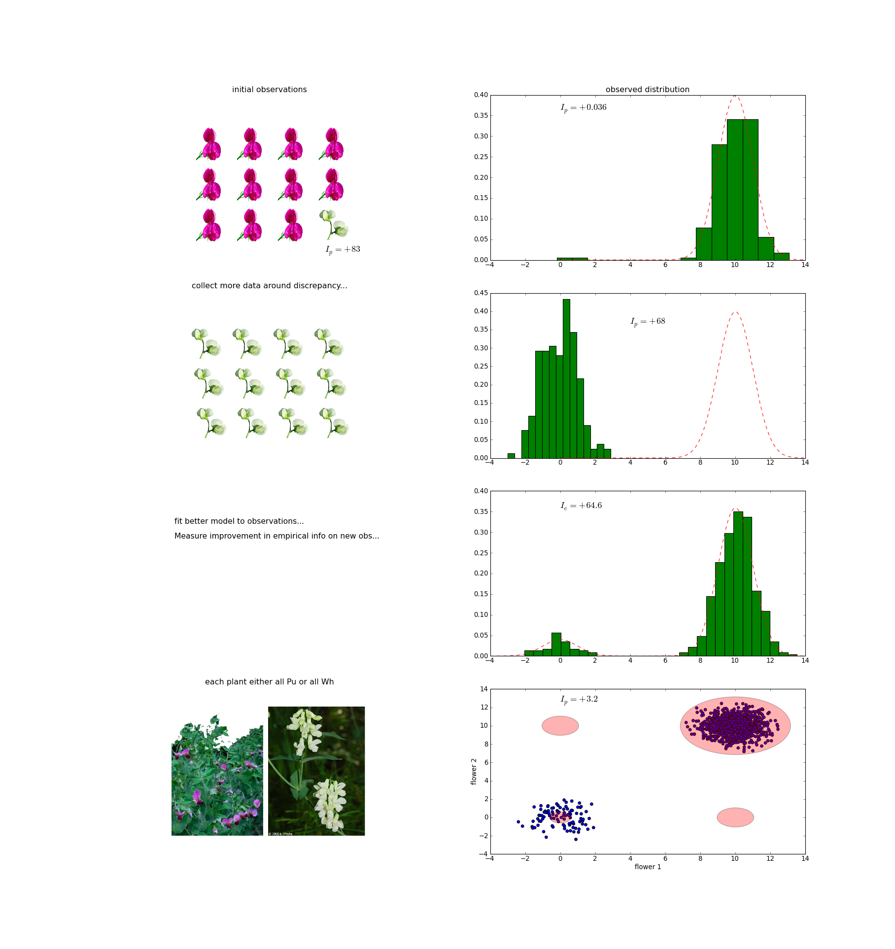
Figure 1: Data collection and model refinement guided by potential information A. Detection of a single outlier datapoint is insufficient to raise the confident lower-bound estimator of $I_{p}$, but suggests that collecting more observations in the region of the surprising data point could yield very large potential information. B. When Mendel observes more flowers from this plant, he finds that all of them are white. This produces +68 bits of potential information. C. To attempt to convert this potential information to empirical information, Mendel updates the pea-species model to reflect the ratio of white vs. purple flowers observed so far. This converts most of the potential information to empirical information. D. However, this species model treats each pea plant as drawn from the same distribution (the pea-species model). But instead each plant appears to have one of two different “phenotypes”: either all its flowers are purple, or all white. This mismatch vs. the model is reflected in strong positive potential information.

Now a second phase begins: seeking to convert this potential information into new empirical information, by adding new model terms that may fit it better. Typically the first step of this is to try to use the current model framework to fit as well as possible. Let’s say RoboMendel has only a simple model of species, in which each species represents a cluster of observable traits (e.g. flower color; shape etc.), and each individual is simply drawn from the probability distribution for its species. In other words, the only variable associated with an individual is what species it appears to belong to, and the only place we can try to tune to “fit” the observations better is the pea-plant species model itself. In this case we could do that by modifying it so that the probability distribution for flower color adds a small peak for white flowers (e.g. representing 10% of the total density, if that’s the fraction of our pea flower observations to date that have been white). We then test this new model by taking a new set of observations and calculating the empirical information yield (relative to our old model). RoboMendel does this and obtains +64.6 bits of empirical information. Is he done?

No, the $I_{p}$ calculation on the new data still indicates +3.2 bits of potential information. The new “mixture model” treated each flower as an independent event (purple or white), whereas in the real observations we see that the white flowers are segregated to just two individual plants (that are all-white), while the remaining plants are all-purple. The lower bound $I_{p}$ estimator indicates that this is not an artifact of insufficient sampling; collecting a larger sample will not make it go away. Instead, it indicates a convincing failure of the model. Note that the $I_{p}$ calculation did not need to be programmed to look specifically for this kind of hidden order; it was simply detected automatically as a reduction in the empirical entropy.

2.3.3 Model Evolution: Prototype, Superset and Posterior Likelihood

To understand this process of model evolution in a general way, we need clear terminology for distinguishing several of its aspects. First, we refer to the set of all possible models that are consistent with past observations as the model superset. Concretely, every model $\Psi$ with $I_{p}(\Psi|obs)<\epsilon$ (for some negligibly small value of $\epsilon$) is a member of this superset. Thus the only constraint on such models is that they yield the same likelihood distribution for the observables collected so far (they can of course differ not only in their hidden parameters but also in their likelihood distributions for other observables not yet collected). Of course, this set is a purely abstract construct, in that its members are innumerable (there is no limit to the complexity of models we could propose).

Instead of trying to explicitly enumerate the model superset, modelers typically propose a single specific model that fits the data. We will refer to such a model as a prototype model; by definition it is a member of the model superset. The value of a good prototype model is easily summarized:

• modelers generally seek the simplest model that fits the data (Occam’s razor).

• This simplicity makes the model predictive; that is, it generally asserts a simple sufficient statistic that it claims is the only variable that matters; all other variables are asserted to be conditionally independent of the observations given this sufficient statistic. This claim is a prediction; that is, it predicts a likelihood distribution for what we should observe under a variety of different experiments. To the extent that this likelihood distribution outperforms the empirical distribution estimated directly from the raw observations, we refer to this prediction power as model information $I_{m}$ [4] .

What happens when we detect strong potential information in a new set of observations vs. our current favored prototype model? First, this means that our model superset shrinks, to no longer include that prototype. We can of course construct a new model to fit these observations. To demonstrate that this new model actually improves prediction power ($I_{e}$) requires collecting a new, independent dataset (testing the model on the same dataset that was used to select the model would violate the definition of $I_{e}$). This should involve both independent replicates of the original experiment (this tests the model’s predictive power for interpolation), and completely new experiments where the model predicts a divergent likelihood than the previous model (we refer to this as extrapolation).

How to compute the expected information yield from such experiments? The de Finetti mixture concept is crucial to this calculation; that is, we must regard the current probability of the new prototype model as significantly less than 1, for obvious reasons:

• the new prototype model was constructed by fitting the data – it has not yet been validated by an independent test dataset;

• it must be considered to be only a subset of current model superset, i.e. we could easily make up many other models that also fit the data. Assuming that some probability measure exists on this model superset space, the new prototype model’s prior probability should certainly be less than 1.

• note that if we asserted a probability of 1 for the model, any validation experiment would by definition have zero expectation information value (because successful validation could not change our predictions at all).

Intuitively, the de Finetti mixture probability for the model $p(\psi_{1})$ determines the information yield of new experiments as follows:

• we construct a weighted likelihood $\psi_{PL}=p(\psi_{1})\psi_{1}+(1-p(\psi_{1}))\psi_{0}$, where $\psi_{0}$ represents the most plausible “counter-model” to the proposed prototype; typically it is just the original prototype model. Thus the contrast between $\psi_{0}$ vs. $\psi_{1}$ indicates specifically how the new model makes new predictions. (Of course, this can be generalized to more than two competing models $\psi_{0},\psi_{1},\psi_{2}...$ etc.)

• because the weight $p(\psi_{1})$ will change in response to each new observation, we refer to the weighted likelihood function $\psi_{PL}$ as the posterior likelihood.

• successful validation experiments (i.e. that confirm the new model) drive up $p(\psi_{1})\to 1$ and thus change our overall prediction $\psi_{PL}$, producing positive information value.

2.3.4 Model Mixture Weighting Schemes

We summarize three distinct schemes for choosing mixture weights in such de Finetti mixture models:

1. Empirical posteriors: in cases where there is a historical record of multiple observations that are relevant to the mixture, the mixture weights are estimated as a posterior probability distribution from those observations. Example: Say RoboMendel has recorded a set of observations of different individual animals that allow him to identify each one’s species. Next he discovers a new species. Based on all his observations, he can estimate the frequency of his new species.

2. A new distinction: if the previous observations do not distinguish the old vs. new models, we may use an uninformative prior. Example: RoboMendel has observed progeny from many matings of pairs of a given species (the progeny looked like the same species as their parents, as predicted by the LFLS model). Now he observes $Wh\times Pu\to Pu$, which does not fit LFLS. So he proposes a new model that fits this observation (e.g. if the “father” was Pu and the “mother” was Wh, he could propose that only the father determines the child’s traits). Note that in all previous observations, since the parents were from the same species, both models make the same prediction. Thus the previous observations provide no basis for estimating the frequencies of the new vs. old models. Only the $Wh\times Pu$ experiment distinguishes them, but since the “father-only” model was constructed to fit the results of this experiment, we can hardly treat it as evidence that any other distinguishing experiment is 100% guaranteed to support “father-only” too. Instead, it seems safer to adopt the conservative position of an uninformative prior, assigning equal probability to the two models. We will often use this weighting scheme in the RoboMendel experiments later in this paper.

3. An arbitrary proposal: say we propose a new model without any basis in potential information, i.e. the existing model already fits the observations, so the new model cannot improve the fit. This becomes a question of the prior probabilities of the models, which strongly favor simpler models (Occam’s Razor, based on the fact that the number of possible models goes up exponentially with their complexity, and their prior probability must be normalized over all such models). We will not use such arbitrary models in this paper.

2.3.5 The Expectation Potential Information Metric

We formalize our experiment planning metric in terms of the expectation value of the potential information of a specific experiment, under our current estimate of the probability of different possible “true distributions” $\omega_{1},\omega_{2},...$ (which we may consider to be the different possible “hidden states” of a random variable $\Omega$ representing the “true distribution”):

$$E(I_{p}(X|\Psi))=\sum_{i}{p(\omega_{i}|\Psi)D(\omega_{i}(X)||\Psi(X))}$$

where $p(\omega_{i}|\Psi)$ represents the probability estimate under our current model $\Psi$ that the true distribution of $X$ will turn out to be $\omega_{i}(X)$.

It is instructive to consider the case where these probability estimates converge to their true values, i.e. $p(\omega_{i}|\Psi)\to p(\omega_{i})$:

$$E(I_{p}(X|\Psi))\to\sum_{i}{p(\omega_{i})\sum_{X}{\omega_{i}(X)\log{\frac{\omega_{i}(X)}{\Psi(X)}}}}$$

$$=\sum_{i,x}{p(\omega_{i},X)\log{\frac{\omega_{i}(X)}{\sum_{i}{p(\omega_{i}|\Psi)\omega_{i}(X)}}}}$$

But the denominator is simply the marginal probability $\sum_{i}{p(\omega_{i})\omega_{i}(X)}=p(X)$. So

$$E(I_{p}(X|\Psi))\to\sum_{i,x}{p(\omega_{i},X)\log{\frac{\omega_{i}(X)p(\omega_{i})}{p(X)p(\omega_{i})}}}=\sum_{i,x}{p(\omega_{i},X)\log{\frac{p(X,\omega_{i})}{p(X)p(\omega_{i})}}}=I(X,\Omega)$$

i.e. the mutual information of the observable $X$ and the hidden variable $\Omega$ representing the true, unknown distribution. The mutual information is a fundamental measure of the “informativeness” of the observable for distinguishing the hidden states, and has been proposed as the metric for choosing an optimal experiment design [8] [9] [3] [10] [11] . The obvious problem is that the true distribution $p(\omega_{i})$ is unknown, and thus we cannot compute the mutual information as traditionally defined. However, we can compute the expectation potential information based on our subjective estimates of $p(\omega_{i}|\Psi)$. $E(I_{p}(X|\Psi))$ represents our subjective estimate of the likely information value of experiment $X$ given our current model $\Psi$. In the limit where our subjective estimates of $p(\omega_{i}|\Psi)$ converge to the true values $p(\omega_{i})$, then our subjective estimator of the experiment’s value converges to the classical “objective” measure given by the mutual information $E(I_{p}(X|\Psi))\to I(X;\Omega)$. We discuss this connection further in the Conclusions.

2.3.6 Disambiguation

If the observable $X$ can determine the hidden state of $\Omega$ unambiguously, i.e. if there is no overlap between the different likelihood distributions $\omega_{i}(X)$, then this further reduces to an even simpler case that we will refer to as disambiguation. Since

$$I(X;\Omega)=H(\Omega)-H(\Omega|X)$$

if $H(\Omega|X)\to 0$ (i.e. observing $X$ determines $\Omega$ unambiguously), then $I(X;\Omega)\to H(\Omega)$. In other words, the information value of the experiment simply becomes equal to our initial uncertainty about $\Omega$. Since good experimental design generally strives to attain an unambiguous determination, disambiguation is a common scenario. This also makes mathematically explicit why repeating an experiment rapidly reduces its information value; the initial experiment eliminates or greatly diminishes the uncertainty and thus the information value of repeating the experiment.

2.3.7 Example: Mouse x Lion

This experiment directly tests the LFLS model, which predicts that no offspring should result from an inter-species cross. The observable “result” from the experiment is whether the cross produces viable progeny or not. We assume that the possible observable states progeny vs. no-progeny can be unambiguously distinguished. The probability estimates of our current model are $\Psi(\text{progeny})=1-p(\text{LFLS})$, $\Psi(\text{no-progeny})=p(\text{LFLS})$. To keep things simple, we consider two possible outcomes of the experiment: if LFLS is true, then we will observe $p(\text{no-progeny})=1$ (i.e. this cross will never produce progeny); if LFLS is false, we will observe $p(\text{progeny})=1$ (every mating successfully produces progeny). So our expectation potential information is:

$$E(I_{p})=p(\text{LFLS})D(p(X|\text{LFLS})||\Psi)+(1-p(\text{LFLS}))D(p(X|\text{not-LFLS})||\Psi)$$

$$=p(\text{LFLS})\left(1\log{\frac{1}{p(\text{LFLS})}}\right)+(1-p(\text{LFLS}))\left(1\log{\frac{1}{1-p(\text{LFLS})}}\right)$$

$$=H(LFLS)$$

This simply reflects our assumption that the observable (progeny vs. no-progeny) can unambiguously determine the hidden state (LFLS vs. not-LFLS). As we noted above, this reduces the expectation $I_{p}$ to a simple disambiguation, where the experiment’s information yield is simply equal to the initial uncertainty about the hidden state.

For p(LFLS) = 0.999, $E(I_{p})\approx 0.01$ bits. The obvious point is that since our current belief in LFLS is already strong, an experiment testing it yet-again is expected to have low information value.

2.3.8 Example: Wh x Wh

This experiment tests whether Wh is heritable; under the LFLS model, if Wh is heritable (i.e. a distinct species), its children will also be Wh. To test this prediction, RoboMendel can simply cross a white-flowered plant with itself, grow the resulting seeds, and observe the resulting flower colors. If he were confident that Wh was definitely a distinct species, this would just be a test of LFLS and would have a low expectation $I_{p}$ yield like the previous case. However, his current belief p(same-species) = 0.5 introduces uncertainty into what we expect to see in this experiment. Specifically, if Wh-heritable then he expects Wh progeny; on the other hand if same-species he expects Pu progeny. So as a simple initial model he adopts $\Psi(Wh)=\Psi(Pu)=0.5$. The expectation information yield is

$$E(I_{p})=p(\text{Wh-heritable})D(p(X|\text{Wh-heritable})||\Psi)+(1-p(\text{Wh-heritable}))D(p(X|\text{not-Wh-heritable})||\Psi)$$

However, the definition of his targeted information metric excludes the second term (which represents the case where Wh is not heritable), so the yield is reduced to the first term:

$$E(I_{p})=-p(\text{Wh-heritable})\log{p(\text{Wh-heritable})}$$

Under his initial assumptions, this gives an expectation yield of 0.5 bits. Clearly RoboMendel would prefer this experiment over Mouse x Lion.

2.3.9 Distinguishing an Experiment’s Information Rate vs. Total Capacity

When the competing models overlap significantly in their likelihood distributions, a single observation is not sufficient to unambiguously determine the hidden state. In this case we can repeat the experiment until the result becomes unequivocal. This is a general principle: we can define the total information capacity of an experiment as the limit of information yield as the number of replicates of the experiment $n\to\infty$. Furthermore, we can define the growth of the information yield as a function of increasing $n$ as the experiment’s information yield curve. Finally, we can define the slope of this curve at a given point as the information rate.

In general, factors that are independently sampled in each replicate of the experiment affect the information rate, but not the total, whereas factors that remain constant over different replicates of the experiment (such as the experiment design itself) affect the total yield. Note that the information rate has critical importance for computing the efficiency of an experiment defined as its information yield per unit cost. This is determined by the experiment’s initial setup cost $c_{s}$ and its unit cost per replicate $c_{r}$.

Concretely, how do we actually calculate information yield curves? Conceptually, we simply replace the single-observation variable $X$ with a vector $\vec{X}^{n}$ representing $n$ observations of $X$. For many problems, the $n$ dimensional vector $\vec{X}^{n}$ can be represented without loss of information by its sufficient statistic $T(\vec{X}^{n})$, which simplifies the computation. We then compute $E(I_{p}(\vec{X}^{n}|\Psi))$ or $E(I_{p}(T(\vec{X}^{n})|\Psi))$ for different values of $n$.

Information Rate Example

Consider a simple experiment to test whether Wh and Pu belong to “the same species”, by crossing them and planting the resulting seeds (if any) to see if they grow successfully (Fig. 2). Imagine that there is a 30% probability that “bad weather” will occur during the experiment, blocking any seeds from growing (regardless of whether they are fertile). If an experiment yields progeny (seeds grow) the result is unambiguous (“Wh and Pu are the same species”), but if no seeds grow we have uncertainty as to whether Wh and Pu are different species, or simply bad weather occurred. Since each experiment has an independent probability of bad weather, if we simply repeat the experiment multiple times, we can reduce this uncertainty to any level we wish. Thus, the bad weather factor affects the experiment’s information rate, but not its total information capacity. Next, consider the effect of adding a control to our experiment that explicitly tests for bad weather. For example, we could also plant seeds of a cross that we know should grow (e.g. $Pu\times Pu$); if they fail to grow, we know bad weather occurred. Adding this control improves the experiment’s information rate, but has no effect on its total information capacity.

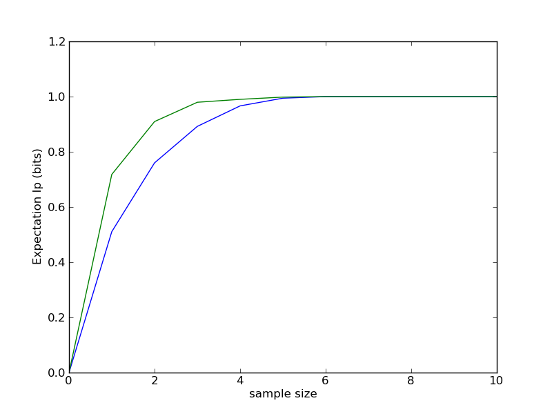
Figure 2: Expectation Ip Yield Curve for Wh x Pu Test In the absence of a control (blue) vs. with Pu x Pu control (green). Assumes 30% probability of bad weather in each experiment; 50% probability that Wh and Pu are same species vs. different species.

Information Total Example: “Technical Failure”

In many fields, “technical problems” can cause an experiment to fail to give the predicted result even if the hypothesis is correct. For example, in molecular biology, a lengthy experiment such as knocking out a gene in mouse can simply give a negative result (no apparent phenotype), e.g. because another pathway exists that can complement the target gene function. Indeed, in complex, incompletely characterized systems such as biology, any one of a myriad of unpredictable problems can cause an experiment to fail: e.g. the sample is lacking a factor that is crucial for the desired reaction; the sample is insufficiently pure and is contaminated with an inhibitor that blocks the reaction; the sample is “too old” and has been degraded by the action of proteases or nucleases; etc. Typically, such technical problems cause a “negative result” that looks the same as would be expected if the hypothesis were false. As the probability of such technical problems increases, the expectation information yield decreases for two reasons: first, the probability of an unambiguous “confirmation” (the observed outcome matches that predicted by our hypothesis) decreases; second, the “failure” outcome (the observed result does not fit the prediction) becomes more and more ambiguous, i.e. it may not mean that the hypothesis is wrong, it may simply mean that a technical problem occurred.

Such “technical failures” affect the total $E(I_{p})$ yield (rather than just the rate), because the cause of the failure is built into the experiment design itself. Simply repeating the same experiment many times will not allow us to sample over independent draws of failure vs. no-failure; if the design is flawed, then every replicate will fail in the same way. Say we are testing a boolean hypothesis $\Psi$ with prior probability $p(\psi^{+})=\alpha$ using an experiment design with failure probability $f$. If the experiment yields a boolean observation $x^{+}$ vs. $x^{-}$, then the joint probabilities are $p(\psi^{+},x^{+})=\alpha(1-f)$ (true positive); $p(\psi^{+},x^{-})=\alpha f$ (false negative); $p(\psi^{-},x^{-})=1-\alpha$ (true negative). We can compute the total expectation potential information for this design as the mutual information $I(\Psi;X)$, which decreases to zero with increasing $f$ (Fig. 3).

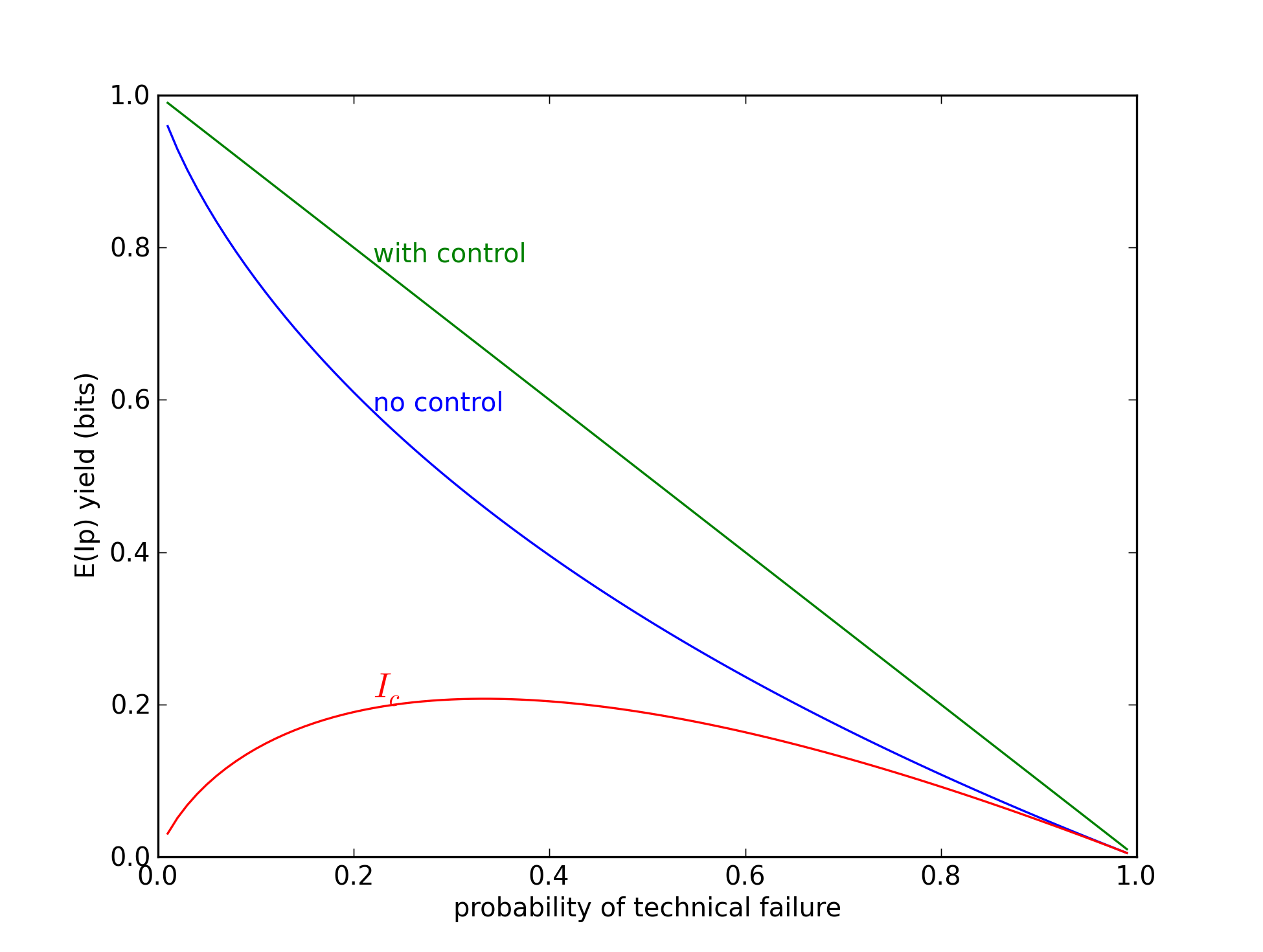
Figure 3: Reduced total expectation potential information as a function of increasing probability of technical failure in an experiment design $E(I_{p})$ with a positive control (green) vs. without a positive control (blue); the difference constitutes the control information $I_{c}$ (red). Assuming an uninformative prior for the hypothesis i.e. $\alpha=0.5$ (see text for details).

This analysis also can measure the value of adding a “positive control” to the experiment. If we add an observable $C$ that yields value $c^{-}$ in the case of technical failure, and $c^{+}$ otherwise, the joint probabilities become $p(\psi^{+},x^{+},c^{+})=\alpha(1-f)$ (true positive); $p(\psi^{+},x^{-},c^{-})=\alpha f$ (false negative); $p(\psi^{-},x^{-},c^{+})=(1-\alpha)(1-f)$ (true negative); $p(\psi^{-},x^{-},c^{-})=(1-\alpha)f$ (true negative). This yields a strictly linear decrease in information yield; thus we can associate with the positive control the amount of $E(I_{p})$ it “rescues” (relative to the experiment lacking the positive control); we refer to this as the control information $I_{c}$ (Fig. 3).

2.3.10 Targeted Potential Information

So far we have ignored the question of whether the observable outcomes are actually of interest. In other words, we have presented universal metrics that treat all observables as “equally valuable” as targets for prediction. It is useful to consider the case where we wish to target our information metric to a specific set of phenomena. For example, for the RoboMendel problem, we wish to restrict the metric to traits that are actually genetic (i.e. which depend on ancestral traits, as opposed to other, environmental factors). We accomplish this in the simplest way possible: we just multiply the expectation information yield for a given observable $X$ by our probability estimate $\tau_{X}$ that it matches our target definition:

$$E(I_{p}(X,Y,Z...|\Psi,\tau))=\tau_{X}E(I_{p}(X|\Psi))+\tau_{Y}E(I_{p}(Y|\Psi))+\tau_{Z}E(I_{p}(Z|\Psi))+...$$

For example, when RoboMendel first encounters a pea plant with white flowers (Wh), there are many potentially interesting questions he could investigate, but he has fundamental uncertainty whether Wh is even a “genetic phenomenon” (i.e. whether this trait is genetically heritable). If not, gaining prediction power for this trait has zero value for his targeted information metric. This initial uncertainty has two effects. First, it reduces the estimated information yield for the many possible experiments he could perform on Wh, because they are down-weighted by an initial $\tau_{Wh}=0.5$ (we will use uninformative priors throughout for such “initial uncertainty” values). Second, it creates strong potential information for any experiment that can test whether Wh is heritable, for the following reason.

2.3.11 Example: An Environmental Factor Control

It is useful to make explicit the factors that could confound this analysis. RoboMendel’s targeted information metric focuses on genetically heritable variation, as opposed to variation caused by environmental factors. Suppose Wh is caused by an environmental factor such as chemicals in the soil. That would confound our interpretation of the Wh x Wh experiment; specifically, if we obtain a Wh child, we are uncertain whether that means Wh-heritable, or simply that the environmental effect occurred. Assume that p(Wh-env) is the probability that any given plant is turned Wh by the unknown environmental factor. (Clearly we do not expect that p(Wh-env) is 100%, since most of our pea plants are Pu). Now our model becomes $\Psi(Wh)=(1+p(\text{Wh-env}))/2$.

This reduces our expectation information yield (Fig. 4). In particular, it reduces the information rate, but not the total information capacity of this experiment. Say we repeat this experiment $n$ times. If Wh-heritable, we expect to get a Wh child every time. However, the probability of that outcome under the environmental factor model is just $p(\text{Wh-env})^{n}$, so our combined model becomes $\Psi(Wh^{n})=(1+p(\text{Wh-env})^{n})/2$.

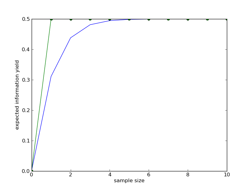
Figure 4: Expectation Ip Yield Curve for Wh x Wh Test In the absence of a control (blue) vs. with Pu x Pu control (green). Assumes 30% probability of environmental factor in each experiment; 50% probability that Wh is heritable.

Next, consider the effect of adding a Pu x Pu control, in other words, planting a seed of a Pu x Pu cross immediately next to the Wh x Wh seed. If Wh is due to an environmental factor in that patch of soil, then both of the resulting plants will be Wh, whereas if Wh-heritable then only the Wh x Wh plant will be Wh, and the control will be Pu. This control enables us to unambiguously eliminate the possibility of an environmental effect even with a single experiment (see figure).

3 RoboMendel Experiment Planning

We now apply these basic concepts and metrics to the RoboMendel experiment planning problem. To show how the metrics work in practice, we first apply them to specific experiments. We then use the metrics to investigate the “research path” (the sequence of experiments chosen by the maximum $E(I_{p})$ metric) under different model assumptions. Source code for the calculations for each specific experiment is available from https://github.com/cjlee112/darwin. Section 5 also provides a very brief summary of the calculation methods for the reader to understand them “at a glance”.

3.1 A Standard RoboMendel Experiment Set

One basic advantage of the RoboMendel problem is that it is possible to easily enumerate all the possible experiments, which are simply all possible crosses of various species. We now list a set of “standard” experiments that RoboMendel will compute expectation information yields for at each stage of the experiment planning process. We state each experiment in terms of the basic cross, and the observed data obtained if the experiment is performed. We use the simple genetics simulation classes included in the darwin empirical information metrics software package [4] to simulate these experiments.

• Mouse x Lion: described above. Outcome: no offspring. Note that this is a generic example of any arbitrary species-cross experiment; other possible inter-species crosses would give the same expectation $I_{p}$ yield.

• Wh x Wh: described above. Outcome: Wh offspring. May include Pu x Pu control to test for possible environmental effects.

• Wh x Pu: outcome, purple-flowered offspring, Hy in the nomenclature below.

• Wh father x Pu mother vs. Wh mother x Pu father: outcome, purple-flowered offspring.

• Pu father x Pu mother vs. Pu mother x Pu father: outcome, purple-flowered offspring. This design simply makes explicitly obvious that the “swap” experiment has no value unless the mother and father have different traits.

• Pu x Pu self-cross (cross a Pu individual to itself). Outcome: for each heterozygous locus, 1/4 of the offspring will be homozygous.

• Hy x Hy: outcome, 1/4 Wh, 1/4 Pu, 1/2 Hy offspring.

• Wh x Hy: outcome, 1/2 Wh, 1/2 Hy offspring.

• Pu x Hy: outcome, 1/2 Pu, 1/2 Hy offspring.

Of course, it must be emphasized that RoboMendel does not any know these outcomes, but simply chooses an experiment to perform (based on the $E(I_{p})$ yield for all these experiments), performs the experiment, and collects observations. Of course, these data will in turn change the expectation information yields for all of the experiments (for example by altering RoboMendel’s probability estimates for p(Wh-heritable), p(same-species), p(LFLS), etc.). RoboMendel therefore recomputes the $E(I_{p})$ yields, chooses the next best experiment to perform, and the cycle repeats.

3.2 The RoboMendel Experiment Sequence

3.2.1 Experiment 1

Starting from RoboMendel’s initial uninformative parameters, it computes the following expectation information yields for the standard experiments:

Table 1: Expectation potential information yields from the initial conditions

Experiment	$E(I_{p})$
Wh x Wh	0.5 bits
Wh x Pu	0.09 bits
Mouse x Lion	0.01 bits
Wh x Pu swap	$1.2\times 10^{-6}$ bits
Pu x Pu swap	0 bits
Pu x Pu self-cross	0 bits

Comments: the Wh x Pu experiment yields are reduced by strong uncertainty about both same-species and Wh-heritable. The Wh x Wh experiment gives a strong yield, because RoboMendel is completely unsure what its result will be, and because it can reveal whether Wh is heritable.

RoboMendel chooses to perform the Wh x Wh experiment, and obtains 100% white-flowered progeny. As the sample size (number of progeny) $n\to\infty$, this causes $p(\text{Wh-heritable})\to 1$. To keep this discussion simple, we skip over these details and assume that at the termination of the experiment $p(\text{Wh-heritable})=0.999$.

3.2.2 Experiment 2

This leads to a new set of expectation information yields:

Table 2: Expectation potential information yields after Wh x Wh experiment

Experiment	$E(I_{p})$
Wh x Pu	0.19 bits
Mouse x Lion	0.01 bits
Pu x Pu swap	0.001 bits
Wh x Wh	0.001 bits
Pu x Pu self-cross	0 bits
Wh x Pu swap	0 bits

Comments: the Wh x Wh yield drops near zero because the previous results convinced us that Wh is heritable (so there is no uncertainty what the outcome of repeating this will be). The Wh x Pu yield has doubled because our uncertainty about Wh-heritable was eliminated.

RoboMendel therefore performs the Wh x Pu experiment and obtains 100% purple-flowered progeny. The fact that progeny were produced at all is only consistent with the same-species hypothesis. Again ignoring the details of sample size, we assume that RoboMendel performed a large enough experiment to obtain a reasonable degree of confidence, leaving him with $p(\text{same-species})=0.999$

We will refer to the progeny of this experiment as Hy (hybrid), since they represent a potentially new category (the offspring of Wh and Pu, parents that do not “look like” they belong to the same species, at least according to our current pea species model). This adds some new possible crosses to the list of experiments.

3.2.3 The One-Parent Model

The asymmetry of this experimental result (the offspring resemble one parent but not the other) raises questions about what exactly the role of both parents is in determining the child’s traits. Previously, such questions did not arise because both parents were drawn from the same distribution. One possible explanation of this result would be if there was a simple asymmetry in which only one parent’s traits were actually passed on to the child. For example, if RoboMendel’s Wh x Pu experiment crossed Wh mothers (flowers) with Pu fathers (pollen), he might interpret the result as indicating that only the father determines the child’s traits. Note that this is irrelevant to all previous experiments (where both parents resemble each other). Therefore RoboMendel proposes this new variant of the LFLS model, with an uninformative prior of p(one-parent)=0.5.

3.2.4 Experiment 3

RoboMendel computes a new set of expectation information yields on this basis:

Table 3: Expectation potential information yields after Wh x Pu experiment

Experiment	$E(I_{p})$
Wh x Pu swap	1.0 bits
Mouse x Lion	0.01 bits
Pu x Pu swap	0.001 bits
Wh x Wh	0.001 bits
Pu x Pu self-cross	0 bits
Wh x Pu	0 bits

Comments: RoboMendel’s uncertainty about whether LFLS might actually only depend on one parent makes the swap experiment highly informative (a straightforward disambiguation of a question with 50% uncertainty). Note that it receives its full expectation Ip value because RoboMendel is now confident of both same-species and Wh-heritable.

RoboMendel therefore performs the swap experiment, and obtains 100% purple-flowered progeny regardless of which parent is Wh vs. Pu. Assume RoboMendel’s sample size is large enough to reduce the one-parent model to p(one-parent)=0.001.

3.2.5 The Transmission Model

RoboMendel therefore considers the next level of model, specifically a Markov model in which each individual receives a “signal” from each of its parents, and transmits one of these signals to each of its children. By definition, Pu sends a pu signal, and Wh a wh signal. Thus the transmission model predicts that since Hy received 1 wh + 1 pu signal, it will send wh with 50% probability and pu with 50% probability to its children. This implies a necessary corollary that pu is dominant over wh, so an individual containing both (like Hy) will be purple-flowered. The conventional terminology for this is to call Wh a recessive trait. Again, RoboMendel assigns this model an uninformative prior of p(transmission)=0.5.

Note that the real significance of this model is that it introduces a hidden variable into our genetic model. That is, it postulates that the inheritance of traits is determined by “signal states” which are not necessarily directly observable. Specifically, it postulates that even though Hy is purple-flowered (and looks no different than Pu), it contains a hidden wh signal.

3.2.6 Experiment 4

RoboMendel computes a new set of expectation information yields on this basis:

Table 4: Expectation potential information yields after Wh x Pu swap experiment

Experiment	$E(I_{p})$
Hy x Wh	1 bits
Hy x Hy	0.98 bits
Mouse x Lion	0.01 bits
Pu x Pu swap	0.001 bits
Wh x Wh	0.001 bits
Pu x Pu self-cross	0 bits
Wh x Pu	0 bits
Wh x Pu swap	0 bits
Hy x Pu	0 bits

Comments: both the Hy x Hy and Hy x Wh experiments receive high expectation Ip values, because for a reasonable sample size (e.g. $n=20$) they turn into a straightforward disambiguation of two distinct predictions (according to LFLS, Hy should yield offspring that resemble it (i.e. 100% should be purple-flowered); whereas transmission predicts that 25% of its progeny should receive two wh signals and therefore should be white-flowered). Note that Hy x Pu gives no expectation information, since both models predict the same observable outcome (100% purple-flowered progeny).

RoboMendel chooses to perform the Hy x Hy and Hy x Wh experiments simultaneously (they can both be done at the same time). The results fit the transmission model, and reject the LFLS model (at least for the Wh/Pu trait).

3.2.7 The Value of Predictions

The transmission model has correctly predicted the behavior of one genetic trait. As we emphasized earlier in this paper, this does not prove that it will hold true for all genetic traits. Instead, this must be viewed as an unknown de Finetti mixture which we can only learn empirically, i.e. to test experimentally what fraction of genetic traits obey the transmission model. Concretely, how can we best do this?

The transmission model itself suggests an experiment that can begin to answer this question. If any additional traits exist in the population that obey this model, we should be able to reveal them easily by a self-cross experiment. That is, additional recessive traits like Wh may be present in the population but hidden because they are infrequent, and therefore very unlikely to occur in both copies in any individual (which would be necessary for it to produce a visible effect). The key prediction of the transmission model is that any self-cross (in which an individual is mated with itself) will reveal approximately one-quarter of its recessive traits in each of its children. That is, just like for Hy x Hy, each recessive trait has a 1/4 probability of transmitting two copies of itself to a given offspring. Thus the transmission model predicts that the self-cross experiment is an effective way to see whether any additional “Mendelian” traits actually exist in the population.

Once again, RoboMendel’s assessment of the value of this experiment depends on his prior probability for this novel event. As before, we assume an uninformative prior, that is p(more-traits)=0.5. How can RoboMendel calculate an expectation information yield for “unknown traits”? The key is that the $E(I_{p})$ doesn’t require predicting exactly what a novel trait will look like; it only requires an estimate of its relative entropy vs. RoboMendel’s current model of a Pu x Pu cross. RoboMendel only has one example mutant trait (Wh) to build such an estimate upon. Wh was observed to be 10 standard deviations divergent from the Pu distribution on one variable (flower-color) but apparently identical to Pu in its distribution of other variables (e.g. plant size; number of leaves; shape of leaves etc.). We therefore imagine modeling a similar “single-variable divergence” as follows. Following our p(more-traits) prior, we assign 50% of the probability to an uninformative density on this variable (we reserve the remaining 50% for the standard Pu peak for this variable). In order to cover deviations as large as Wh in both directions, the uninformative part of this density is of the form $p(X)=0.5/20$ for $X\in[0,20]$. Under such a model the relative entropy of a trait like Wh would be $D(Wh||\Psi)=\log 40-H(X|Wh)\approx 3.27$ bits.

Therefore the expectation $I_{p}$ yield for finding one such trait with probability p(more-traits)=0.5 is approximately 1.64 bits. Note this assumes generating enough progeny from a given individual (e.g. $n=20$) for strong confidence of getting at least one child with two copies of the putative trait (with 25% probability per child).

Note that this expectation yield is a direct consequence of the de Finetti mixture model. That is, we selected the transmission model to fit a single instance of a genetic trait. But this single instance does not prove that the model will be a “universal law” that applies to all genetic traits. Instead, according to the de Finetti mixture there is an unknown mixture of trait types (some of which may obey this model, and others which obey different models). The associated probabilities have a crucial effect on the model’s total prediction power, depending on whether most traits obey it vs. very few. (Taking the transmission model as a specific example, even today researchers struggle with the question of what proportion of important human disease traits are “simple” (involving only a few mutations / genes; in the simplest case, Mendelian) vs. “complex” (in which a disease susceptibility arises from a combination of small effects of many genes)). According to the de Finetti view we can only learn these mixture probabilities empirically, e.g. by testing different genetic traits to see if they obey this model. Based on a single case where we selected the transmission model to fit the data, we have little basis for estimating this mixture, so initially we use an uninformative prior.

This considerably changes the expectation yield for the self-cross experiment. Previously it had zero value, because RoboMendel’s current model confidently expected a single outcome (Pu children, just as would be predicted for any Pu x Pu cross). Now, however, it provides a powerful way to test a hypothesis that RoboMendel is currently very uncertain about (i.e. whether any more traits will obey the transmission model).

Another question is how many distinct individuals RoboMendel should perform the self-cross experiment on; this depends on the (unknown) frequency of such traits in the population. Again using Wh as a guide, it seems reasonable to use approximately the same number of individuals in which the Wh trait was first found, say approximately 20 - 100 plants. In this way, RoboMendel would have the same power for detecting an additional trait as was used for discovering the original Wh trait.

3.2.8 Experiment 5

RoboMendel obtains a new set of expectation information yields on this basis:

Table 5: Expectation potential information yields after Hy x Hy/Wh experiments

Experiment	$E(I_{p})$
Pu x Pu self-cross	1.64 bits
Mouse x Lion	0.01 bits
Pu x Pu swap	0.001 bits
Wh x Wh	0.001 bits
Hy x Hy	0.001 bits
Hy x Wh	0.001 bits
Wh x Pu	0 bits
Wh x Pu swap	0 bits
Hy x Pu	0 bits

RoboMendel therefore performs the Pu x Pu self-cross experiment and inspects the progeny for clearly anomalous characteristics. Based on historical data, this experiment would be highly likely to discover additional recessive traits such as those found by Mendel: Wrinkled seeds; White seed coats; Yellow seeds; Yellow pods; Constricted pods; Terminal flowers; Short plants; etc.

3.3 What If RoboMendel Fails to Propose the Transmission Model?

The above sequence demonstrates the power of proposing a good model: it predicts new experiments that lead to further discoveries. This suggests an obvious question: what would have happened if RoboMendel had not considered the transmission model after the Wh x Pu experiment? Certainly, alternative models are possible.

3.3.1 Alternative Model: “Pu Undilutable”

For example, RoboMendel could simply have proposed that “Pu always beats Wh“, in the sense that any child with a purple-flowered parent and a white-flowered parent will always have purple flowers. (Note that this is different than saying that Wh is recessive in the transmission model). We now consider this alternative experiment sequence.

The essence of this model is that Pu is “undilutable”: no matter how much Wh we “dilute” it with (i.e. how many times we cross it with Wh), we will still get 100% Pu progeny. This suggests an obvious experiment: serially “dilute” Pu by crossing it over and over with Wh. If the new Pu-undilutable model is correct, these successive generations will remain 100% purple-flowered; otherwise we might expect increasing amounts of Wh progeny to begin appearing. Following our previous practice we assign the new model an uninformative prior p(Pu-undilutable)=0.5. Note that we already have the first step in this “dilution sequence”: Hy, the result of crossing “pure” Pu to Wh once. Concretely, we would like to complete at least a few “dilution cycles” with large enough sample sizes in each generation to detect a small fraction of Wh children. Say each cross produces 30 seeds from which new plants can be grown. If Pu were a chemical compound, its concentration would be diluted 30-fold each generation. If RoboMendel repeats this dilution over 10 generations, Pu will be diluted by a factor of $5.9\times 10^{14}$, which would appear to be a rigorous test of the dilution model. RoboMendel therefore computes the expectation information yield of this experiment as simple disambiguation of a hypothesis with 50% uncertainty, which yields 1 bit.

Thus Hy x Wh becomes RoboMendel’s next experiment step (highest expected yield). It yields an unexpected result: half Wh progeny, and half purple-flowered progeny. Not only is Pu-undilutable immediately rejected, but this result makes clear that RoboMendel must hypothesize a “hidden” variable representing an individual’s genetic state (since two plants that outwardly looked the same, Hy and Pu, behaved completely differently genetically). Note that introducing a “hidden variable” to represent the genetic state is the essence of the transmission model. Thus, failing to propose the transmission model, but continuing to use information metrics to find the best test of alternative models, has forced RoboMendel back towards the transmission model.

3.3.2 Alternative Model: An Inter-Species Hybrid?

We now consider another alternative explanation of the Wh x Pu result. Mendel and contemporaries were aware that in some cases crosses of highly similar species (e.g. horse and donkey) could produce viable progeny (e.g. $\text{horse}\times\text{donkey}\to\text{mule}$), but that these progeny were generally sterile (i.e. unable to reproduce). Thus RoboMendel could propose an alternative explanation that the Wh x Pu result does not imply same-species, by asserting that Hy is a “hybrid cross” of two different species. This model suggests an obvious test: Hy x Hy, to see if progeny are obtained. Assigning this species-hybrid model an uninformative prior of 0.5, the Hy x Hy experiment becomes a straightforward disambiguation with a 1 bit expected yield. RoboMendel therefore performs this experiment as his next best step.

Even with progeny from a single Hy x Hy cross (approximately 30 plants), RoboMendel is almost certain to obtain at least one Wh child (since each child actually has a 25% chance of being Wh). This both rejects the species-hybrid model and again compels the concept of a “hidden variable” describing genetic state (since again Hy is behaving very differently from Pu genetically, even though it looks exactly the same in appearance).

Once again, using expectation information to pick experiments that will test the model has overcome a wrong initial choice of model, and forced RoboMendel back in the direction of the transmission model.

4 Conclusions

Recently, there has been growing interest in automated experiment planning in general [12] [13] and specifically in mutual information for optimal experiment planning [9] [14] [3] [10] [11] . The approach presented in this paper is largely compatible with previous results on mutual information as an experiment planning metric, although it starts from rather different foundations. The mutual information approach focuses on the question of how informative a given experiment (observable variable $X$) is about a designated hidden variable $\Omega$ (the target of interest). By contrast, potential information is defined strictly in terms of the likelihood of observable variables (measuring our prediction power on these observables, not our ability to infer hidden variables). It is a striking result that the expectation potential information (defined in these purely observable terms) can converge to the mutual information. This follows from the de Finetti mixture of competing models in the $E(I_{p})$ calculation; when the estimated mixture weights converge to the true model probabilities, the expectation potential information converges to the true mutual information $E(I_{p})\to I(X;\Omega)$. Of course, in real scientific inference problems, the true model probabilities are unknown.

Ordinarily, the mutual information metric is applied to problems where the hidden variable target (“what question to ask?”) is pre-defined, and the experimental observation (“how to answer it?”) is varied, to find the best experiment for determining the value of the hidden variable. As an example of this distinction, consider the behavior of the general mutual information metric $I(X;\Omega)$ as we repeat an experimental observation of $X$ again and again. By definition, $I(X;\Omega)$ remains constant after these multiple observations, even though the past observations may have already told us the actual value of $\Omega$. This behavior is not suitable for helping us decide “what question to ask?”. By contrast, the expectation potential information goes to zero if an observation is repeated in this way, reflecting the fact that there is nothing more to learn from repeating this experiment. In this respect it behaves more like a conditional mutual information taking into account all previous observations.

In this paper we have addressed both types of challenges together. Expectation potential information is defined in terms of the possible gain in prediction power (ability to predict observables) that could result from performing an experiment. This definition subsumes the issues not only of how best to answer a given question, but also what question will be most valuable to ask (i.e. will yield the largest possible increase in prediction power). Concretely, we have demonstrated the utility of $E(I_{p})$ for choosing the “best next question” among very different experiments (e.g. mouse $\times$ lion, $Wh\times Pu$ etc.). We have presented evidence that the expectation potential information metric is useful both for guiding experiment proposal (choosing what experiment to do next, out of all the possibilities), and for fine-grained experiment optimization (such as deciding whether a given control is worth including or not). It generalizes nicely from single observations to multiple replicate observations, providing straightforward measures of both information rate and total information yield.

We suggest that the main value of an experiment planning metric is when it acts as a “gradient” on the space of all possible experimental observations. In other words, it provides a purely local signal (computable at any given point on an experiment planning trajectory) that indicates how to “read” the largest increase in average prediction power from this space. Thus it breaks down the problem of guessing the hidden structure of this space, into small steps for reading the patterns in the data, ideally one dimension at a time. (Of course, this signal must be present in the data in the first place; if the observations were encrypted with a one-time pad, no such breakdown would be possible).

The RoboMendel problem illustrates this process in action. The initial detection of a potential information signal (white flowers on a pea plant descended from purple-flowered parents) indicates a breakdown of the current model, and suggests plausible modifications of the model. Computation of expectation potential information identifies the best experiments to test these plausible models. An important feature of such a metric is robustness: ideally it should point you in the right direction regardless of what path you take to get there. For example, in addition to considering the “canonical” path (in which RoboMendel proposes the “transmission” model that Mendel himself proposed), we also considered several alternative paths in which RoboMendel proposed alternative, incorrect models. We showed that $E(I_{p})$ then identified experiments to test these models, which produced observations that rejected these models and directly revealed the “transmission” pattern. This at least illustrates the kind of robustness that we would hope for from a general information metric.

As such, this metric could be applied to enable RoboMendel to discover many additional features of genetics. Note that Experiment 5 (Pu x Pu self-cross) would directly lead to identifying the next layer of genetics, namely multiple genetic loci controling multiple traits. From this point, the exact same $E(I_{p})$ experiment planning process should be able to discover the obvious substructure and superstructure of these traits, e.g. discovering complementation groups i.e. “genes”; discovering chromosomes; constructing genetic maps; discovering pathways and epistasis etc.

Of course, it must be emphasized that far more is required for actual automated experiment planning and discovery [12] . Here we have only discussed an information metric for forecasting the yield, given specific proposed models and experiments. That entirely ignores the crucial questions of how to generate model proposals in an automatic and appropriate way, and robust principles for assigning their de Finetti weights (prior probabilities). In the RoboMendel example we have also largely ignored the question of how to generate experiment proposals (this clearly must be driven by looking for the predicted differences between the new vs. old models). Another major area that we’ve ignored is the question of experiment costs. Presumably, to choose the experiment with the highest information yield per cost requires good models of the structure of experiment costs, e.g. distinguishing setup costs and latency for beginning an experiment vs. the unit cost of adding one more sample replicate. We point out these large areas of research merely to emphasize that the information metric presented here is but a small piece of the whole puzzle.

4.1 The Scientific Method

Karl Popper emphasized that a scientific hypothesis must be testable to be useful [15] . Thus the value of a hypothesis is that it makes predictions that both differ from our previous expectations (otherwise they would be indistinguishable), and are readily verifiable by available experimental means.

The expectation potential information metric is entirely consistent with this outlook. In order for an experiment to produce potential information, it must have two or more observationally distinguishable outcomes, and there must be strong uncertainty about which outcome will actually occur. Translating this into Popper’s terms, this means that the hypothesis under test must predict a different outcome than our previous model, and there must be uncertainty about the hypothesis (leading to uncertainty about the expected outcome).

The RoboMendel example illustrates how the scientific method translates into a cycle of steps driven by the basic information metrics of potential information and expectation potential information. We enumerate the basic steps:

1. a surprising observation: substantial potential information is detected (via a confident lower bound on the $I_{p}$ metric [4] ).

2. a new model that fits: a modification to the current model is proposed, typically by fitting the new, surprising observation(s). Note that the new model should not differ from the old model on previous sets of observables (which the old model fit well).

3. a divergent prediction: the new model can only improve prediction power if it makes some different predictions than the old model, and if we have significant uncertainty about their de Finetti mixture weights. Actually testing one of these predictions will have information value to the extent it can result in changing the de Finetti weights. We quantify this as the $E(I_{p})$ metric.

Since the purpose of the $E(I_{p})$ metric is to maximize the potential information yield, performing the experiment it chose to test the model’s predictions often leads to new potential information, e.g RoboMendel’s tests of the “one-parent” model or the “Pu undilutable” model both lead to surprising observations (that do not fit the model). Then we resume the cycle again at step 1.

4.2 The “Boolean Logic” of Expectation Potential Information

The expectation potential information principle imposes an interesting constraint on information yields from experiment planning. Whereas an “accidental” observation can produce a huge $I_{p}$ yield (e.g. seeing white flowers on a pea plant yields approximately 68 bits), the expected yield from a planned experiment tends to be limited to $E(I_{p})\to\log{N}$ where $N$ is the number of distinct models it can distinguish. Indeed, in the common situation where we are testing a new model vs. the old model, every “good” experiment becomes at most a 1 bit hypothesis test. In this sense, $E(I_{p})$ comes very close to a Boolean logic, in which the scientific method becomes a series of “true vs false” hypothesis tests. This may seem surprising, given that the metric is based strictly on observation log-likelihoods, which have no finite limit (if the model fits the observations poorly, $I_{p}$ can grow arbitrarily large). It is the expectation principle that strongly constrains the metric: it can take into account the possibility of a hugely surprising experimental outcome, but by definition assigns it a vanishingly small probability. Thus the biggest $E(I_{p})$ yield comes not from such “big” surprises but instead from “little” surprises (i.e. with 50% probability).

However, it’s worth noting that there are some exceptions to this simplistic “Boolean” pattern. First, it doesn’t apply automatically to any arbitrary model proposal, even if one can design an experiment that would test it. Unless there is potential information (observations) favoring the new model over the old model, there is no justification for assigning it a large (50%, uninformative) probability. Indeed, arbitrary complex models are likely to be assigned small prior probabilities (simply to satisfy normalization of their priors; c.f. Occam’s razor), and thus to receive correspondingly small $E(I_{p})$ values. Second, the risk of “technical failure” problems in the experiment design can reduce either the total $E(I_{p})$ or the information rate far below 1 bit (e.g. see the Technical Failure example in section 2.3). Third, if we are computing a targeted information metric, it may be reduced far below 1 bit (even for a good experiment) if there is strong uncertainty that the observation is relevant to the target of interest (e.g. if RoboMendel is interested in inheritance, he initially has uncertainty whether Wh is actually a heritable trait). On the other hand, the targeted information yield might be far larger than 1 bit, if the new model gives predictions not only for the one observable being tested, but for many other relevant observables as well (for example, RoboMendel’s transmission model yields improved prediction power not only for Wh x Pu but for many other traits). Fourth, one could of course test many plausible models in one experiment design, which would yield an $E(I_{p})$ much greater than one bit. As an extreme example, imagine a botanist planning a return expedition to a new continent, based on having discovered many new species on his two previous expeditions there. In effect the “new models” being tested are the set of all possible new botanical species, and the previous expeditions provide reasonable confidence that the “experiment design” can detect many of these “big surprises” (i.e. accurately observe their surprising traits). In principle, we could empirically estimate a very large $E(I_{p})$ for the return expedition, from the observed $I_{p}$ yields from the previous expeditions.

5 Methods Summary

We have already presented the $E(I_{p})$ computations at length in the theory section (Section 2), and all details of the calculations are available as source code for the information metric values presented in this paper (available from https://github.com/cjlee112/darwin). Here we simply provide a quick reference summarizing the calculations for Section 3 so readers can understand them “at a glance”.

Expectation potential information: $I_{p}$ is an empirical (sample-based) estimator of the relative entropy of the true (but unknown) observation likelihood $\Omega(X)$ vs. the model observation likelihood $\Psi(X)$. To compute its expectation value for a set of possible likelihood distributions $\omega_{i}(X)$ with estimated mixture weights $p(\omega_{i}|\Psi)$, we compute the potential information yield for each possible experiment “outcome” $\omega_{i}(X)$ vs. the original mixture model which we define as $\psi_{PL}(X)=\sum_{i}{p(\omega_{i}|\Psi)\omega_{i}(X)}$:

$$E(I_{p})=\sum_{i}{p(\omega_{i}|\Psi)D(\omega_{i}(X)||\psi_{PL}(X))}$$

where the relative entropy $D(\omega_{i}(X)||\psi_{PL}(X))$ is defined as usual

$$D(\omega_{i}(X)||\psi_{PL}(X))=\sum_{X}{\omega_{i}(X)\log{\frac{\omega_{i}(X)}{\psi_{PL}(X)}}}$$

for a discrete variable $X$ (or replaced by an integral over $X$ if it is a continuous variable).

Targeted information metric: to restrict the information metric to a target phenomenon (e.g. genetic inheritance), we re-weight the $E(I_{p})$ for a given observable $X$ by the probability $\tau_{X}$ that $X$ is indeed an exemplar of that target phenomenon. For example, at the beginning of the RoboMendel experiments, there is strong uncertainty as to whether Wh is in fact a genetic trait (that can be inherited, as opposed to an environmental phenomenon). We calculate the expectation targeted information value as

$$E(I_{p}(X|\Psi,\tau))=\tau_{X}E(I_{p}(X|\Psi))$$

References

- 1. Shannon C (1948) A mathematical theory of communication. Bell System Technical Journal 27: 379-423.
- 2. Kullback S, Leibler R (1951) On information and sufficiency. The Annals of Mathematical Statistics 22: 79-86.
- 3. Paninski L (2005) Asymptotic theory of information-theoretic experimental design. Neural Computation 17: 1480-1507.
- 4. Lee C (2011) Empirical information metrics for prediction power and experiment planning. Information 2: 17-40.
- 5. Akaike H (1974) A new look at the statistical model identification. IEEE Trans Automat Contr AC-19: 716-23.
- 6. Schwarz G (1978) Estimating the dimension of a model. Ann Stat 6: 461-464.
- 7. de Finetti B (1937) La prévision: ses lois logiques, ses sources subjectives. Ann Inst Henri Poincaré 7: 1–68.
- 8. Lindley D (1956) On a measure of the information provided by an experiment. Ann Math Statist 27: 986-1005.
- 9. Machens CK (2002) Adaptive sampling by information maximization. Phys Rev Lett 88: 2281040.
- 10. Lewi J, Butera R, Paninski L (2009) Sequential optimal design of neurophysiology experiments. Neural Computation 21: 619-687.
- 11. Cavagnaro DR, Myung JI, Pitt MA, Kujala JV (2010) Adaptive design optimization: A mutual information-based approach to model discrimination in cognitive science. Neural Computation 22: 887-905.
- 12. King RD, Rowland J, Oliver SG, Young M, Aubrey W, et al. (2009) The automation of science. Science 324: 85-89.
- 13. Guan Y, Dunham M, Caudy A, Troyanskaya O (2010) Systematic planning of genome-scale experiments in poorly studied species. PLoS Comp Biol 6: e1000698.
- 14. Nelson JD (2005) Finding useful questions: on bayesian diagnosticity, probability, impact and information gain. Psych Rev 112: 979-999.
- 15. Popper K (1959) The Logic of Scientific Discovery. Basic Books, New York, NY.