Measurements of electron anisotropy in solar flares using albedo with RHESSI X-ray data

Abstract

The angular distribution of electrons accelerated in solar flares is a key parameter in the understanding of the acceleration and propagation mechanisms that occur there. However, the anisotropy of energetic electrons is still a poorly known quantity, with observational studies producing evidence for an isotropic distribution and theoretical models mainly considering the strongly beamed case. We use the effect of photospheric albedo to infer the pitch angle distribution of X-ray emitting electrons using Hard X-ray data from RHESSI. A bi-directional approximation is applied and a regularized inversion is performed for eight large flare events to deduce the electron spectra in both downward (towards the photosphere) and upward (away from the photosphere) directions. The electron spectra and the electron anisotropy ratios are calculated for broad energy range from about $10$ and up to $\sim 300$ keV near the peak of the flares. The variation of electron anisotropy over short periods of time intervals lasting 4, 8 and 16 seconds near the impulsive peak has been examined. The results show little evidence for strong anisotropy and the mean electron flux spectra are consistent with the isotropic electron distribution. The $3\sigma$-level uncertainties, although energy and event dependent, are found to suggest that anisotropic distribution with anisotropy larger than $\sim 3$ are not consistent with the hard X-ray data. At energies above $150-200$ keV, the uncertainties are larger and thus the possible electron anisotropies could be larger.

1 Introduction

Solar flares are one of the most energetic processes which occur in the solar system. However the details of the acceleration processes responsible are still poorly known. The X-rays which are observed at the Earth are commonly produced by the accelerated electrons interacting with the solar plasma and producing bremsstrahlung radiation. To understand solar flares it is therefore important to understand the distribution of these accelerated electrons. In general, this distribution will vary in space, energy and in pitch angle (see 2011SSRv..159..107H, 2011SSRv..159..301K, as the recent reviews of electron properties in solar flares).

Several techniques have been used to estimate the anisotropy in the pitch-angle distribution of X-ray emitting electrons in solar flares [Holman et al. (2011), Kontar et al. (2011)]. The most commonly used method is to look at the centre-to-limb variation of solar X-ray properties [Datlowe, Elcan, and Hudson (1974), Vestrand et al. (1987)]. That is comparing the characteristics, most commonly total X-ray flux [Pizzichini, Spizzichino, and Vespignani (1974)], or the spectral index of solar flares at the limb to disk centre events. Studies concentrating on lower energy emission (below 300 keV) tended to find no significant evidence of directivity. These studies have also been performed using SMM data [Dennis (1988)] studying flares with energies above 300 keV [Vilmer (1994), Bai (1988), Bogovalov et al. (1985)]. Some evidence for directivity at high energies has been reported [McTiernan and Petrosian (1991), Vestrand, Forrest, and Rieger (1991)]. More recently RHESSI (Ramaty High Energy Solar Spectroscopic Imager) data [Lin et al. (2002)] has been used to determine the X-ray anisotropy [Kašparová, Kontar, and Brown (2007)]. An obvious disadvantage of the statistical method is that the variation can only be seen as an average over a large number of solar flares, so little can be said about X-ray or electron anisotropy in a given flare.

An approach which allows individual flares to be studied is the stereoscopic method [Catalano and van Allen (1973)]. Here each individual flare is measured directly by two spacecraft at two different locations, ideally well separated in space. Studies that have been performed using this method do not show any clear evidence of directivity [Kane et al. (1998), Li et al. (1994)]. A disadvantage of this approach is the difficulty in cross calibrating, often leading to large errors. Another drawback is, as in the centre-to-limb method, this technique does not give direct information about the downward electron distribution.

As an anisotropic electron distribution will produce polarised X-rays, measuring the polarisation can therefore give a measure of the anisotropy of the electron distribution [Leach and Petrosian (1983)]. An isotropic source should show low polarisation, whereas a beam should produce significant polarisation [Bai and Ramaty (1978), Leach and Petrosian (1983), Emslie, Bradsher, and McConnell (2008)]. Studies of polarisation have been performed using various X-ray satellites, recently using the Coronas-F satellite [Zhitnik et al. (2006)]. The reported measurements vary substantially from observation to observation, adding to the scepticism of these measurements. A major drawback of this approach is the observational difficulty in measuring polarisation at HXR energies for transient events like solar flares. Several attempts have been made using RHESSI [McConnell et al. (2002), Suarez-Garcia et al. (2006)], but so far there have been no conclusive measurements made. HXR polarisation has not yet been used to its full potential and future observations could provide a more definitive answer.

Another important process, which can be used to diagnose the angular distribution, is photospheric albedo [Kontar and Brown (2006)]. Photospheric albedo of X-rays results from initially downward directed X-rays, which are Compton scattered off electrons in the solar photosphere, being observed at Earth. This effect distorts the HXR spectrum [Tomblin (1972), Bai and Ramaty (1978)] and leads to an appearance of apparent low energy cutoff in the deduced electron spectrum [Kontar, Dickson, and Kašparová (2008)], when the observed X-ray spectrum is not corrected for an albedo [Kontar et al. (2006)]. As the spectral shapes of reflected and primary hard X-ray spectra are sufficiently distinct, these two components can be distinguished and the albedo reflected flux could be used as a measure of the downward going electrons (Figure 1). RHESSI provides sufficient energy resolution, broad energy coverage, and sensitivity to better constrain directivity of energetic electrons in individual solar flare events.

Here we use this albedo method to examine the directivity of energetic electrons in solar flares. We first perform some forward modelling to examine the effect directivity of the electron spectrum and the role of the albedo contribution has on solar flare spectra. The RHESSI flare catalogue has been searched for suitable flares between 2002 and 2008 and we use the spectral data from the impulsive phases of several well observed flares to perform a bi-directional inversion, estimating the fluxes of electrons travelling towards and away from the photosphere.

2 Solar flare spectrum and electron anisotropy

The spatially integrated X-ray photon flux spectrum at the Earth $I(\epsilon,\theta_{0})$, [photons cm^-2 s^-1 keV^-1] is straightforwardly related to the mean electron flux spectrum of energetic electron ${\overline{F}}(E,\beta)$ [electrons  cm^-2 s^-1 keV^-1 sr^-1] via the linear integral relation (e.g. 2004ApJ…613.1233M, 2011arXiv1110.4993J). For a given electron distribution ${\overline{F}}(E,\beta)$, where $\beta$ is the electron pitch angle, the resulting emitted X-ray flux at distance $R$ is

$$\ilabel{eq:Idef}I(\epsilon,\theta_{0})=\frac{{\bar{n}}V}{4\pi R^{2}}\int_{0}^{2\pi}\int_{0}^{\pi}\int_{\epsilon}^{\infty}{\overline{F}}(E,\beta)Q(\epsilon,E,\theta(\beta,\phi))sin(\beta)dEd\beta d\phi\;~{},$$ (1)

where $V$ is the source volume, $\bar{n}$ is the mean plasma density, $Q(\epsilon,E,\theta)$ is the angular dependant bremsstrahlung cross-section, $\epsilon$ is photon energy, $E$ is electron energy and $\theta$ is the angle between the initial electron velocity vector and the direction of the emitted photon. The cross-section used here is the electron-ion cross section, formula 2BN from 1959RvMP…31..920K with Coulomb correction by 1939AnP…426..178E added. The relation between the angles $\beta$, $\theta_{0}$, $\phi$ and $\theta$ is given by

$$cos\theta=cos\beta\,cos\theta_{0}+sin\beta\,sin\theta_{0}\,cos\phi\;~{},$$ (2)

where $\theta_{0}$ is the angle between the emitted photon and the direction of the photosphere. The exact plasma density distribution $n$ and flaring volume $V$ are often poorly known and therefore it is preferable if the value ${\bar{n}}V{\bar{F}}(E,\Omega)$ is inferred, this is the mean electron flux spectrum [Brown, Emslie, and Kontar (2003)], a density weighted electron flux, multiplied by ${\bar{n}}V$ the number of electrons in the emitting volume. This value is model independent, and its detailed structure can be related to the electron acceleration and propagation physics which is central to the understanding of solar flares.

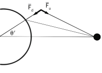
Figure 1.: The geometry of the X-ray emitting source above the photosphere and bi-directional approximation. X-rays are emitted in all directions and observed directly at Earth or Compton back-scattered in the solar photosphere and then observed at Earth. The true angular distribution of electrons ${\overline{F}}(E,\beta)$ is approximated by downward $F_{d}$ and upward $F_{u}$ going electrons.fig:geo

The electron distribution of emitting electrons is assumed to be separable in energy and angle. The energy dependence is taken to be a single power-law as solar flare x-ray observations are often well fit by power laws implying close to power-law electron spectra. For simplicity the pitch angle distribution is taken to be a gaussian beam centred downwards. This pitch angle distribution is assumed as electrons tend to stream along magnetic field lines resulting in a downwards beam, and the gaussian parametrization of this is popular as it has useful analytic properties. The total distribution has the form similar to 1983ApJ…269..715L

$$\ilabel{eq:mod}{\overline{F}}(E,\beta)\propto E^{-\delta}\exp\left(\frac{-(1-\mu)^{2}}{\Delta\mu^{2}}\right)\;~{},$$ (3)

where $\mu=cos(\beta)$ and $\Delta\mu$ characterises the width of the Gaussian. It should be noted that Equation (3) refers to the mean electron flux spectrum not the injected electron spectrum considered in 1983ApJ…269..715L. Three different cases were assumed for the angular variation of the electron spectrum (Figure 2): the isotropic case ($\Delta\mu=10$), an intermediate anisotropic case ($\Delta\mu=0.4$) and a highly beamed case ($\Delta\mu=0.1$). The electron spectral index $\delta$ was assumed to be $\delta=2$ as the typical flare spectral index of X-rays in large flares is around $\gamma=3$ (see e.g. 1985SoPh..100..465D) and for the mean electron flux spectrum $\gamma\approx\delta+1$.

As the assumed electron distribution has azimuthal symmetry an average cross-section integrated over $\phi$ can immediately be defined leaving only the angles $\theta_{0}$ and $\beta$ needed to characterise the angular distribution (c.f. 2004ApJ…613.1233M)

$$\ilabel{cs}Q^{\prime}(\epsilon,E,\theta_{0},\beta)=\int_{\phi=0}^{2\pi}Q(\epsilon,E,\theta(\phi))d\phi\;~{}.$$ (4)

The angular distribution of the emitted X-rays with respect to the downward direction can now be found by applying this cross section to the assumed electron spectrum and integrating over electron energy and pitch angle (Figure 3)

$$\ilabel{Idef3}I(\epsilon,\theta_{0})=\frac{{\bar{n}}V}{4\pi R^{2}}\int_{0}^{\pi}\int_{\epsilon}^{\infty}{\overline{F}}(E,\beta)Q^{\prime}(\epsilon,E,\beta,\theta_{0})sin(\beta)dEd\beta\;~{}.$$ (5)

The primary emission observed for a flare at heliocentric angle $\theta^{\prime}$ is expected to come from a small range in angle in the direction of the observer. Considering the geometry, it is clear that the upward directed photon distribution can be approximated as

$$I_{U}(\epsilon)=I(\epsilon,\theta_{0}=180^{\circ}-\theta^{\prime})\;~{}.$$ (6)

The albedo reflected component, on the other hand, results from the photons directed down towards the photosphere. This is likely to be a broader distribution so an average is taken over a downwards directed cone concentric with the mean direction of the electron distribution and with half angle $\alpha$, in this study a value of $90^{\circ}$ is used. The downward directed flux can then be defined as

$$I_{D}(\epsilon)=\frac{\displaystyle\int_{\theta_{0}=0}^{\alpha}I(\epsilon,\theta_{0})\sin\theta_{0}d\theta_{0}}{\displaystyle\int_{\theta_{0}=0}^{\alpha}\sin\theta_{0}d\theta_{0}}\;~{}.$$ (7)

The reflected component, due to albedo, of a given X-ray spectrum incident on the photosphere can be characterised by using a Green’s function $A$ dependant on observation angle $\theta^{\prime}$ [Kontar and Brown (2006)]. Thus, the total observed X-ray spectrum will be given by the sum of the directly observed and reflected components:

$$I_{O}=I_{U}+A\;I_{D}\;~{},$$ (8)

where $I_{O}$ is the total and $I_{U}$, $I_{D}$ are upward and downward directed components (Figure 6).

In practice the photon spectrum is calculated numerically with a finite resolution. For energy a pseudo-logarithmic binning scheme with 100 bins starting at $10$ keV and going up to 5 MeV is used for both electrons and photons. Due to the highly anisotropic nature of the cross-section at high energies fine resolution in angle was needed. Angles $\beta$ and $\theta_{0}$ were binned in 90 evenly spaced bins between 0 and $\pi$ whereas $\phi$ was binned in 180 evenly spaced bins between 0 and $2\pi$.

The upward and downward components of the photon flux are now given by vectors. The observer directed component is defined as

$${\bf I_{U}}=\{I_{U}(\epsilon_{i}),...,I_{U}(\epsilon_{n})\},\qquad i=1,..,n$$ (9)

where $\epsilon_{i}$ corresponds to the centre energy of the photon bin and $n$ is the number of bins in photons space. The photosphere directed component is given by ${\bf I_{D}}$ defined in the same way. Similarly the angle dependant Green’s function is here calculated in the form of a $n\times n$ Green’s matrix $\bf A$. The vector representing the total observed flux is simply given by

$$\bf{I_{O}}={\bf I_{U}}+A{\bf I_{D}}\;~{},$$ (10)

where $A$ is the albedo matrix constructed from Green’s functions.

2.1 Photon Spectral Index

Due to the effect of albedo one of the most notable variations with changing anisotropy is in the photon spectral index, the derivative with respect to energy of the photon flux. It is commonly defined as [Brown and Emslie (1988), Conway et al. (2003)]

$$\gamma(\epsilon)=-\frac{\epsilon}{I}\,\frac{dI}{d\epsilon}=-\frac{d\,log\,I}{d\,log\,\epsilon}\;~{},$$ (11)

which is calculated for both the primary photon spectrum for a range of viewing angles (Figure 5) and for the total observed spectrum including albedo component for a range of positions on the solar disk (Figure 7).

Figure 2.: Polar diagrams of the assumed electron pitch-angle distribution $F(E,\beta)$. The angle made with the x-axis corresponds to the pitch angle $\beta$ of the electron and the radial extent corresponds to the magnitude of the distribution. The electron flux with $\mu=1$ is normalised to 1. Left: isotropic case $\Delta\mu=10$. Middle: intermediate anisotropic case $\Delta\mu=0.4$. Right: Highly beamed case $\Delta\mu=0.1$. fig:pole

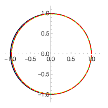
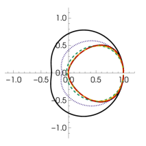
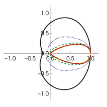
Figure 3.: Polar diagrams of the emitted photon distribution $I(\epsilon,\theta_{0})$. The angle made with the x-axis corresponds to the angle $\theta_{0}$ and the radial extent corresponds to the magnitude of the photon distribution. The energy distribution is plotted for several energies: 10 keV (solid black), 40 keV (dotted purple), 150 keV (dashed green), 600 keV (dashed yellow) and 5 MeV (solid red). The photon flux with $\cos\theta_{0}=1$ is normalised to 1. Left: isotropic case Middle: intermediate anisotropic case. Right: Highly beamed case.fig:polp

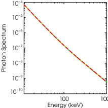
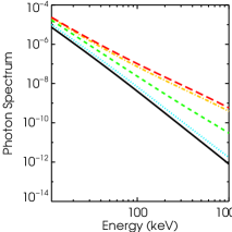
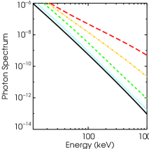
Figure 4.: Photon flux for several selected values of $\theta_{0}$ - $0^{\circ}$ (red, long dashed), $45^{\circ}$ (yellow, dot-dashed), $90^{\circ}$ (green, dashed), $135^{\circ}$ (blue, dotted) and $180^{\circ}$ (black, solid). Left: isotropic case Middle: intermediate anisotropic case. Right: Highly beamed case.fig:modflux

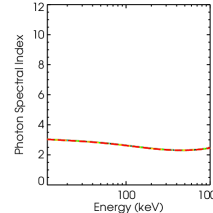
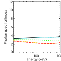
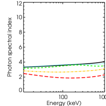
Figure 5.: Photon spectral index for several selected values of $\theta_{0}$ - $0^{\circ}$ (red, long dashed), $45^{\circ}$ (yellow, dot-dashed), $90^{\circ}$ (green, dashed), $135^{\circ}$ (blue, dotted) and $180^{\circ}$ (black, solid). Left: isotropic case Middle: intermediate anisotropic case. Right: Highly beamed case.fig:modgam

This method was performed for the cases of strong ($\Delta\mu=0.1$) and intermediate ($\Delta\mu=0.4$) beaming over an energy range 10 keV to 5 MeV (Figure 2). After applying this assumed electron spectrum to the bremsstrahlung cross-section the angular dependant X-ray emission is found (Figure 3), for lower energies this tends towards being closer to isotropic than the electron distribution but for high energies it is reasonably similar to the input electron spectrum. The emitted flux density (Figure 4) and spectral index (Figure 5) for a range of angles of observation are then calculated. A Green’s matrix corresponding to the albedo reflection at a range of heliocentric angles [Kontar et al. (2006)] was then applied (Figure 6). Emission close to the solar limb shows very little influence from albedo as expected and the power law in photon energy is recovered, however emission closer to the disk centre shows a distinctive hump over the entire energy range due to the albedo reflection. The influence of albedo can be seen more clearly when observed photon spectral index is considered (Figure 7), flares close to the disk centre show a large increase in $\gamma$ above 200 keV, and this is more pronounced in the strong beaming case.

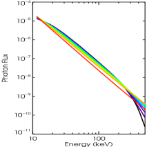
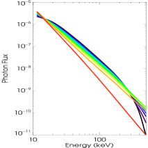
Figure 6.: Total observed photon flux including reflected albedo component for flares located at different places on the disk ranging from disk centre $\cos\theta^{\prime}=1$ (black), $\cos\theta^{\prime}=0.9$ (purple), $\cos\theta^{\prime}=0.8$ (indigo) $\cos\theta^{\prime}=1$ to limb $\cos\theta^{\prime}=0.2$ (yellow) $\cos\theta^{\prime}=0.1$ (orange) $\cos\theta^{\prime}=0.01$ (red). Left: isotropic case Middle: intermediate anisotropic case. Right: Highly beamed case.fig:modtotf

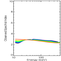
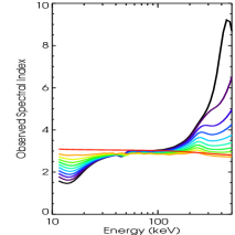
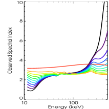
Figure 7.: Photon spectral index for the total observed spectrum against photon energy for flares located at different places on the disk ranging from disk centre $\cos\theta^{\prime}=1$ (black), $\cos\theta^{\prime}=0.9$ (purple), $\cos\theta^{\prime}=0.8$ (indigo) $\cos\theta^{\prime}=1$ to limb $\cos\theta^{\prime}=0.2$ (yellow) $\cos\theta^{\prime}=0.1$ (orange) $\cos\theta^{\prime}=0.01$ (red). Left: isotropic case Middle: intermediate anisotropic case. Right: Highly beamed case. fig:modindex

3 Application to RHESSI data

The RHESSI data archive was examined for flares with emission above $300$ keV with particular attention paid to flares close to the solar disk centre. These flares are selected because the forward modelling suggests that the variation due to beaming is strongest at high energies and flares closest to the disk centre should have the strongest albedo reflection and should therefore also show the greatest change due to beaming. In total eight suitable flares were found (Table 1) which were within $60^{\circ}$ of the solar centre (Figure 8) and showed significant $>3\sigma$ counts above background (Figure 9); a number of other flares matching these criteria were found but they were discounted due to high levels of pulse pileup and particle contamination.

tab:flares

Table 1.: Flares suitable for analysis. flare positions are given in arcsecond from the Sun centre.

	Flare Date	Start Time (UT)	GOES Class	x position	y position	$\mu$
a	20-Aug-2002	08:25:21	M3.4	562	-270	0.72
b	10-Sep-2002	14:52:47	M2.9	-622	-244	0.72
c	17-Jun-2003	22:52:42	M6.8	-783	-148	0.52
d	2-Nov-2003	17:16:00	X8.3	770	-343	0.51
e	10-Nov-2004	02:09:40	X2.5	738	116	0.69
f	15-Jan-2005	22:49:08	X2.6	117	325	0.93
g	17-Jan-2005	09:43:44	X3.8	441	301	0.86
h	10-Sep-2005	21:34:26	X2.1	-667	-255	0.69

Figure 8.: Positions of all 8 flares studied on the solar disk. The inner rings indicate heliocentric angles of $30^{\circ}$ and $60^{\circ}$.

For each of the flares found the background was removed in the standard manner [Schwartz et al. (2002)]. Counts were accumulated over the impulsive phase, as the differences in the spectra due to anisotropy in the electron spectra are greater at higher energies. The time intervals studied were selected ensuring a high number of high energy counts (Figure 10). A pseudo-logarithmic binning scheme between 10 keV and 500 keV was used to initially accumulate the spectra avoiding detectors 2 and 7 due to their poor resolution [Smith et al. (2002)]. After background subtraction had been performed the energy range was further reduced by discarding the energy bins with counts less than $3\sigma$ above the background.

4 Inversion method

The cross-section is similarly divided into two components $Q^{F}$ represents the bremsstrahlung cross-section in the forward direction, that is the radiation beamed in the same direction as the electron was travelling and $Q^{B}$ represents the cross-section for the radiation beamed in the opposite direction to the electron. These matrices are determined by taking the full angular dependant cross-section and averaging over a range of angles similar to the method applied to determine the upward and downward components of the photon flux

$$Q(\epsilon,E,\theta_{0})=\frac{1}{2\pi(1-\cos(\alpha))}\int^{\alpha}_{\beta=0}Q^{\prime}(\epsilon,E,\beta,\theta_{0})\sin\beta d\beta\;~{},$$ (12)

with $\alpha=90^{\circ}$ $Q^{B}(\epsilon,E)=Q(\epsilon,E,\theta_{0}=180^{\circ}-\theta^{\prime})$ and $Q^{F}(\epsilon,E)=Q(\epsilon,E,\theta_{0}=0^{\circ})$

This results in a directly observed count spectrum given by

$$\ilabel{Iobs}I_{o}(\epsilon)=\frac{{\bar{n}}V}{4\pi R^{2}}\int_{\epsilon}^{\infty}(Q^{F}(\epsilon,E){\overline{F}}_{u}(E)\;+\;Q^{B}(\epsilon,E){\overline{F}}_{d}(E))dE$$ (13)

and a downward directed photon flux given by

$$I_{d}(\epsilon)=\frac{{\bar{n}}V}{4\pi R^{2}}\int_{\epsilon}^{\infty}(Q^{B}(\epsilon,E){\overline{F}}_{u}(E)\;+\;Q^{F}(\epsilon,E){\overline{F}}_{d}(E))dE\,.$$ (14)

A Green’s function approach can be used to determine the fraction of this downward directed photon flux reflected back towards the observer by albedo [Kontar et al. (2006)].

The matrix relation between the observed photon spectrum and the bi-directional electron spectra is now given by

$$\ilabel{eq:full}\mathbf{C=S\left(Q^{F}+AQ^{B}\qquad Q^{B}+AQ^{F}\right)\left({\bar{F_{u}}\atop\bar{F_{d}}}\right)}\;~{},$$ (15)

where $\mathbf{A}$ is a discretized matrix representing the Green’s function and $\mathbf{S}$ represents the photon to count spectral response of RHESSI.

Equation (eq:full) must be simplified so that the array containing the cross-section and Green’s functions is converted into a standard two dimensional matrix and the two component electron spectrum is represented as a one dimensional vector. A method of performing this transformation is described in 1995ApJ…448L..61H. The equation can then be solved using the standard regularised inversion methods.

A significant problem is determining the electron spectrum which produced a given photon spectrum. In general there is a linear relationship between the observed count spectrum represented by vector $\mathbf{C}$ and the electron distribution which produced it, $\mathbf{\bar{F}}$, which can be written the form

$$\ilabel{eq:mat}\mathbf{C=MF}$$ (16)

here $\mathbf{M}$ is a matrix defined by $\mathbf{M=SQ}$ where $\mathbf{Q}$ is a matrix representing the bremsstrahlung cross-section in this case $\mathbf{Q=\left(Q^{F}+AQ^{B}\qquad Q^{B}+AQ^{F}\right)}$ To determine the emitting electron spectrum this must be solved for $\mathbf{\bar{F}}$, here this is equivalent to the matrix $\mathbf{\left({\bar{F_{u}}\atop\bar{F_{d}}}\right)}$. However this problem is ill-posed as noise in the data is amplified making a direct inversion impossible [Bertero, Mol, and Pike (1988)]. A technique for solving this is regularized inversion [Tikhonov (1963)].

As Equation (eq:mat) does not have a unique solution additional constraints must be imposed by considering the physical properties of the electron distribution.The solution can then found by solving the Lagrange multipliers problem

$$\ilabel{eq:tik}||\mathbf{M\bar{F}-C}||^{2}+\lambda||\mathbf{L\bar{F}}||^{2}=\mathnormal{minimum},$$ (17)

this method is known as Tikhonov regularisation. Here $\mathbf{L}$ represents the additional constraint, in this case an approximation of the differential operator is used and $\lambda$ is the regularisation parameter, a variable which determines the degree of smoothness imposed on the solution. Equation (eq:tik) can be solved by Generalized Singular Value Decomposition for arbitrary $\lambda$ and $\mathbf{L}$ [Kontar et al. (2004)].

The choice of the regularisation parameter here is determined by examining the normalised residuals which are defined by $r_{k}=(({\bf{M}}{\overline{\bf{F}}})_{k}-{\bf{C}}_{k})/\delta C_{k}$. Then the best value of $\lambda$ by minimizing

$$\ilabel{chi2}\|({\bf{M}}{\overline{\bf{F}}}_{\lambda}-{\bf{C}})(\delta{\bf C})^{-1}\|^{2}=\alpha.$$ (18)

The choice of $\mathbf{L}$ is related to the constraint applied to the solution and in this case should be related to the underlying physics, here a finite difference matrix representing the first derivative is used. dependence The robustness of the solution can be improved if the equation is first preconditioned [Kontar et al. (2004)]. A forward fit performed on dependence the data using a standard model of a thermal component plus a broken power law [Holman et al. (2003)]. This estimated electron spectrum, $\mathbf{{\overline{F}}}_{0}$ , is used as a starting point for the regularised inversion. The inversion is performed on the difference between the data, $\mathbf{C}$ and the fit, $\mathbf{M{\overline{F}}_{0}}$, This modified data vector and the cross-section matrix are also scaled by a factor of $\mathbf{\sqrt{M{\overline{F}}_{0}}}$. These transforms both make the solution much flatter and so less prone to errors.

This method has been applied to the problem of inverting the angle averaged electron spectrum numerous times (e.g. 2006ApJ…643..523B,2005) but can be extended to determine an angular dependant electron flux. This is done here by extending the cross-section matrix to take account of the angular dependence of the bremsstrahlung cross-section and then solving for an electron flux matrix with two components, one directed down towards the photosphere, $\bar{F}_{d}$, and one directed towards the observer $\bar{F}_{u}$ Kontar and Brown (2006).

The inversion algorithm is applied to the selected time intervals of the flare and the upward, ${\bar{n}}V{\bar{F}_{u}}$, and downward, ${\bar{n}}V{\bar{F}_{d}}$, electron fluxes calculated. As a first estimate a thermal plus double power-law fit is performed with ${\overline{F}}_{u}={\overline{F}}_{d}$.

The errors on the electron flux components are calculated by combining the errors on the count flux and the errors on the background. Random perturbations are applied to the count flux based on the error and the electron flux is recalculated. The distribution of these realizations is then used to estimate the error on the electron flux. The regularised solution also has finite resolution. The resolution matrix is defined as $R=M_{\lambda}^{-1}M_{true}$, where ${\overline{F}}_{true}^{-1}=M_{true}C$ is the true solution to the inverse problem and ${\overline{F}}_{\lambda}=M_{\lambda}^{-1}C$ is the regularised solution. The resolution matrix quantifies the horizontal errors of the solution, so the identity matrix (zero horizontal errors) correspond to the direct inverse $M_{\lambda}^{-1}$. For any practical situations, the regularization imposes a spread on the strong peaks centred on the main diagonal, this is an unavoidable occurrence in any inverse problem. The FWHM of each of the rows of this matrix is taken as the energy resolution for that energy bin and is considered here as the horizontal error in the electron flux (Figure 11).

The anisotropy was defined to be the ratio of $nV{\overline{F}}_{d}$ to $nV{\overline{F}}_{u}$. Confidence strips for the total anisotropy were calculated using the same method as the errors in the electron flux (Figure 12). Random perturbations were applied within the ”confidence river” defined by both the horizontal and vertical error bars.

In order to test the method, we have applied it to simulated electron spectra. The electron spectra have been assumed to have simple functional forms and equivalent photon spectra and albedo reflection were added using analytical expressions for electron fluxes. Random noise, at a similar level to the noise estimated from RHESSI observations, has been added to the resulting count spectrum. This simulated spectrum was then inverted using the same algorithm as the real data.

Spectra from isotropic initial distributions generally gives a result which is consistent with the input spectrum within errors and shows a reasonable distribution of residuals. For weak anisotropy the results generally show broader confidence intervals than for the isotropic case with the same level of noise so that the solution is often consistent with the weakly anisotropic input spectrum and an isotropic input spectrum. For stronger levels of anisotropy (${\overline{F}}_{d}/{\overline{F}}_{u}>10$ at 100 keV), the method tends to give unphysical negative values for the electron flux. This can be avoided by increasing the regularisation parameter to force the solution to be smoother and ensure the solution is positive everywhere. However this approach leads to under-regularisation and unacceptably large residuals suggesting that the method cannot converge on a physically meaningful solution which satisfies the data. We emphasise that there is an upper limit to the size of the maximum anisotropy detectable as it is difficult to constrain an anisotropy that is greater than the fractional error in the larger component of electron flux.

The tests also confirm that this method works best for flares with high energy counts close to the disk centre and that the anisotropy cannot be reliably inferred for weak or limb events, as was expected from the forward modelling. All the inversions of RHESSI data show physically sound results with reasonable residuals.

  

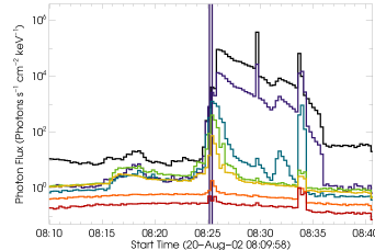
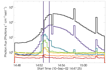
     (a)                                (b)

  

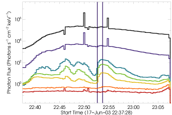
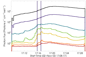
     (c)                                (d)

  

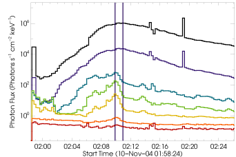
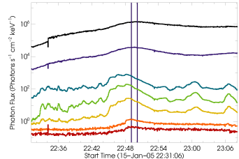
     (e)                                (f)

  

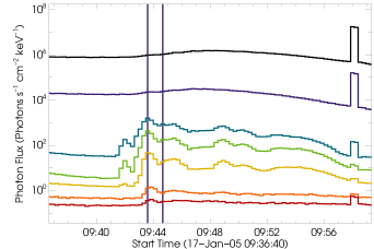
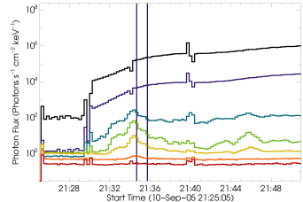
     (g)                                (h)

Figure 9.: RHESSI lightcurves of each of the flares studied in 7 energy bands- black 7-12 keV, purple 12-25 keV, blue 25-50 keV, green 50-100 keV, yellow 100-300 keV, orange 300-800 keV, red 800-5000 keV. The vertical lines show the accumulation time interval used. The plots are semi-calibrated, a diagonal approximation of the RHESSI response is used to estimate the photon flux from the measured counts. There are still instrumental artefacts present with the very sharp spikes and dips being the result of attenuator status changes. All times are in UT. fig:F-panels

  

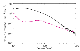
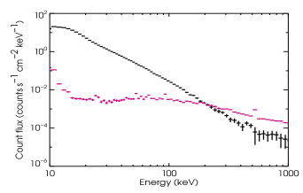
                              (a)                                (b)

  

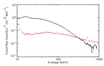
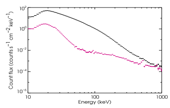
                              (c)                                (d)

  

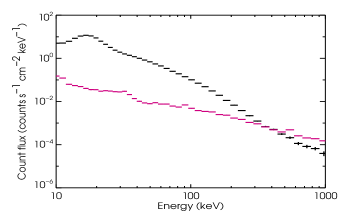
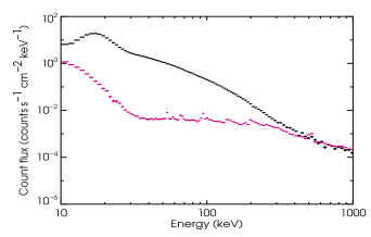
                              (e)                                (f)

  

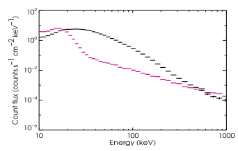
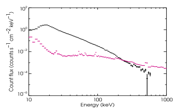
                              (g)                                (h)

Figure 10.: Impulsive phase count spectra accumulated by RHESSI for each flare studied (see Figure 9). The black line shows the background subtracted counts and the magenta line the background. fig:C-panels

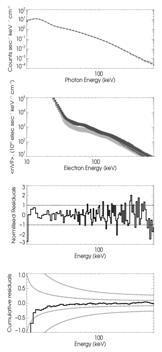
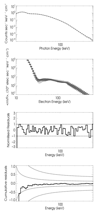
Figure 11.: Results of the invertion procedure for 64 second intervals from two selected flares on 10th November 2004 (left) and 17th June 2003 (right). Top panel shows the measured count spectrum (full line) overplotted with the count spectrum corresponding to the calculated regularised electron spectra (dashed line). The second panel shows regularised electron spectrum with associated 1-$\sigma$ vertical and horizontal error bars for each point, the light grey line denotes the upward electron flux and the dark grey line the downward electron flux. The third panel shows the normalised residuals for each time interval and the bottom panel shows the cumulative residuals.fig:resid

  

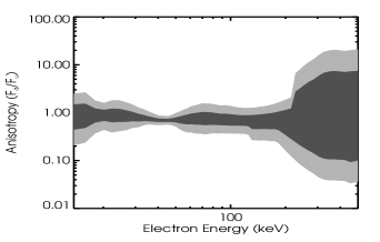
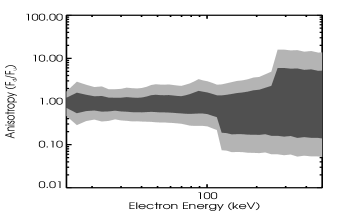
        (a)                                (b)

  

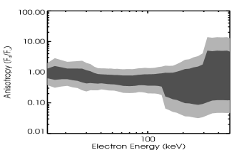
        (c)                                (d)

  

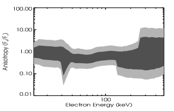
        (e)                                (f)

  

        (g)                                (h)

Figure 12.: The anisotropy of the electron spectrum (defined as ${\overline{F}_{d}}/{\overline{F}_{u}}$) for all eight flares studied. The dark grey area represents the $1\sigma$ confidence interval and the light grey the $3\sigma$ confidence interval. fig:A-panels

  

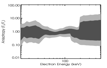
        (a)                                (b)

  

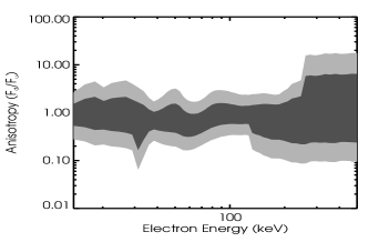
        (c)                                (d)

  

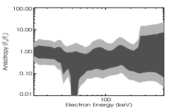
        (e)                                (f)

  

        (g)                                (h)

Figure 13.: The anisotropy of the electron spectrum (defined as ${\overline{F}_{d}}/{\overline{F}_{u}}$) for the first eight 4 second time intervals for the flare occurred on 10 November 2004. The first interval starts at 02:09:40 UT and the intervals shown here cover the most intense part of the impulsive peak. The dark grey area represents the $1\sigma$ confidence interval and the light grey the $3\sigma$ confidence interval. fig:As-panels

Figure 14.: Pitch angle spread, $\Delta\mu$, for various anisotropies ${\overline{F}_{d}}/{\overline{F}_{u}}$ using ${\overline{F}(\mu)}\propto\exp\left(\frac{-(1-\mu)^{2}}{\Delta\mu^{2}}\right)$ (solid line) and ${\overline{F}(\mu)}\propto\exp\left(\frac{-(1-\mu)}{\Delta\mu}\right)$ (dashed line). The vertical dotted line shows an anisotropy of 3. fig:delmu

4.1 20th August 2002

This flare was detected on 20th August 2002 around 08:20 UT with the impulsive peak starting about 08:25 UT. It was detected with a heliocentric angle of $\sim 43^{\circ}$ equivalent to $\mu=0.73$. The flare also shows good count statistics up to 400 keV. As this flare had attenuator status changes from A0 (open telescope) to A1 (thin shutter in) at 08:25:16 UT and to A3 (both shutters in) at 08:25:44 UT, the analysis was only performed over the 16 s period rather than the 64 s period studied for most flares. There is some particle contamination over the impulsive phase. This flare was extensively studied by 2007A&A…466..705K and the background subtraction used in this paper is similar to the subtraction described there. This flare was previously analysed using bi-directional inversion by 2006A&A…446.1157K.

4.2 10th September 2002

This flare was detected on 10th September 2002 between 14:02 and 15:15 UT with the impulsive peak starting about 14:52 UT. It was detected with a heliocentric angle of $\sim 44^{\circ}$ equivalent to $\mu=0.72$. The flare also shows good count statistics up to 300 keV. This flare also has an attenuator status change from A0 to A1 at 14:52:43 UT and to A3 at 14:54:16 UT, so the impulsive phase is taken to be a 32 s time interval between 14:52:47 and 14:53:19 UT.

4.3 17th June 2003

This flare was detected on 17th June 2003 starting at approximately 22:30 UT. As RHESSI shows significant particle contamination during the early stages of this flare analysis was performed on a later impulsive peak with accumulation starting at 22:52:42 UT. It was detected with a heliocentric angle of $59^{\circ}$ equivalent to $\mu=0.51$. The flare also shows good count statistics up to 300 keV.

4.4 2nd November 2003

This flare was detected on 2nd November 2003. It was detected with a heliocentric angle of $\sim 59^{\circ}$ equivalent to $\mu=0.51$. The flare also shows good count statistics up to 300 keV. RHESSI showed some elevated particle levels during the impulsive phase of the flare so analysis was confined to the earlier part of the impulsive phase.

4.5 10th November 2004

This flare was detected on 10th November 2004. It was observed with a heliocentric angle of $46.5^{\circ}$ equivalent to $\mu=0.69$. The flare shows no significant particle measurements during the impulsive phase and low probability of pulse pileup. The flare also shows good count statistics up to 500 keV.

4.6 15th January 2005

This flare was detected on 15th January 2005. It was detected with a heliocentric angle of $20^{\circ}$ equivalent to $\mu=0.93$, the closest of all the flares selected to the disk centre and therefore the most likely to show evidence of strong downwards directivity. The flare also shows good count statistics up to 400 keV.

4.7 17th January 2005

This flare was detected on 17th January 2005 between 09:30 and 15:15 UT with the impulsive peak starting about 09:42 UT. It was detected with a heliocentric angle of $\sim 31^{\circ}$ equivalent to $\mu=0.86$. The flare also shows good count statistics up to 300 keV. As this flare occurs in the tail of a previous flare is has very high background at low energies. Counts below 18 keV were not accumulated for this flare. This flare was also previously analysed using bi-directional inversion 2006A&A…446.1157K.

4.8 10th September 2005

This flare was detected on 10th September 2005. It was detected with a heliocentric angle of $\sim 46^{\circ}$ equivalent to $\mu=0.69$. This flare showed negligible particle contamination and a low probability of pulse pileup. The flare also shows good count statistics up to 300 keV. Due to changes in the attenuator status during the impulsive phase from A1 to A3 at 21:34:12 UT and the maximum time interval studied for this flare is 32 s starting at 21:34:26 UT.

4.9 Short time intervals

Four seconds is roughly the rotation period of RHESSI and thus the shortest time interval studied here. Longer time intervals of 8, 16, and 32 seconds were also studied for some flares depending on the length of the impulsive phase. The results for these time intervals are very similar to the results for the full impulsive phase. The inversions for short time intervals generally show confidence intervals around an anisotropy of 1 at the $1\sigma$ level extending to around 2 below 100 keV and sharply increasing above that. As the count statistics are lower for the shorter time intervals the confidence intervals are wider than for the full impulsive phase. There was no discernible statistically significant variation in the level of anisotropy for the duration of the impulsive phase. As an example the anisotropies for each of the 4 second time intervals for the flare on 10th November 2004 are shown in Figure fig:As-panels.

5 Discussion and Conclusions

This analysis shows consistently that for almost all flares studied by RHESSI that the recovered ${\overline{F}_{d}}/{\overline{F}_{u}}$ is close to unity within the confidence intervals being consistent with an isotropic pitch angle distribution. For almost every flare downward beaming of a ratio greater than $\sim 3:1$ is ruled out to $3-\sigma$ confidence below $\sim 150$ keV. The only clear exception to this is the flare on 20th August 2002 between 30 and 50 keV, where the recovered flux appears to be inconsistent with isotropic at the 3-$\sigma$ level and suggest a slightly greater ($1.5-2$) upward flux. This flare is unusual in several respects. There is a high level of particle contamination throughout the impulsive phase. Several background subtractions were examined to attempt to account for this. This flare is also one of the flattest flares studied, which makes pileup correction more difficult to estimate. Also, this is one of only two flares studied where the attenuator status was A1 for the examined time interval.

These measurements appear to rule out any strong beaming such as would be expected in the basic collisional thick target model. However as only two components are recovered and the confidence intervals can be fairly large using this method, the observations are consistent with a range of possible pitch angle distributions including fully isotropic distributions, pancake distributions and weak beaming below the measured confidence level. The size of the uncertainties could be reduced with better count statistics and better energy resolution as each of these distributions does show different spectral variation. The forward modelling shows very clearly that when there is significant beaming in the emitting electron population it will result in a very strong albedo emission. For many cases with substantial beaming, particularly close to the disk centre, the albedo component can dominate over the primary component. In order to directly compare the measured results to the forward model a plot of $\Delta\mu$ against anisotropy (${\overline{F}_{d}}/{\overline{F}_{u}}$) is included (Figure fig:delmu) both for the functional form described by Equation 3 and for another commonly used form ${\overline{F}}\propto\exp\left(\frac{-(1-\mu)}{\Delta\mu}\right)$. It should be stressed that the results in Figures fig:A-panels and fig:As-panels are model independent and can be interpreted in terms of a variety of models, including, but not limited to those considered in Figure fig:delmu.

These results are consistent with previous published results which showed little evidence of directivity below 300 keV. It should be noted that this study measures anisotropy in terms of the electron flux, whereas for other types of study the parametrisation of anisotropy is often in terms of the directivity of the X-ray emission for stereoscopic studies and the centre-to-limb variance for statistical studies. These are generally related to the electron anisotropy in a model dependant manner. As the X-ray emission can be quite broad, particularly for low energies, a large anisotropy in the electron spectrum could result in a low photon spectrum directivity. 2007A&A…466..705K performed a centre-to-limb study using RHESSI data and inferred a directivity ratio between 0.2 and 5 in the range 15 - 20 keV. As the emission below $\sim 30\,keV$ is expected to be predominantly produced by thermal electrons it is expected that the distribution in this energy range should be isotropic. This is particularly true for the flares on 17 June 2003 and 10 November 2004 which show strong thermal components however this may not be the case for flares which show a weak thermal component such as the flare on 20 August 2002.

As this study measured X-rays in the energy range 10 - 500 keV the reliability of the inversion above approximately 250 keV is questionable. As can be seen from Figure fig:A-panels the confidence interval increases significantly at a few hundred keV. Thus it is difficult to make comparisons with the SMM studies which examined X-ray measurements above 300 keV. However the measurements in this study are for the most part in agreement with previous studies McTiernan and Petrosian (1991).

As electrons propagate through the corona and chromosphere they will be pitch angle scattered by Coulomb collisions (e.g. 1981ApJ…251..781L; 1991A&A…251..693M), although it seems that collisions will be insufficient to isotropise an initially beamed distribution Brown (1972); Leach and Petrosian (1981). These results, therefore, suggest that either the accelerated electron population is more isotropic, or other transport effects are more important than anticipated. Specifically, the electron scattering by various wave-particle interactions could increase the pitch angle spread of the energetic electrons. Further, if the distribution of energetic electrons is close to isotropic, the role of return current should be diminished. In addition we note, that although the return current itself does contribute to the formation of a backward going beam, it is likely to be more efficient at energies below $\sim 50$ keV, so that the higher energy electrons are expected to be weakly affected Holman et al. (2011).

Acknowledgements

This work is supported by STFC, UK. The European Commission is acknowledged for funding from the HESPE Network (FP7-SPACE-2010-263086) (EPK).

References

- Bai (1988) Bai, T.: 1988, Directionality of continuum gamma rays from solar flares. ApJ 334, 1049 – 1053. doi:10.1086/166897.
- Bai and Ramaty (1978) Bai, T., Ramaty, R.: 1978, Backscatter, anisotropy, and polarization of solar hard X-rays. ApJ 219, 705 – 726. doi:10.1086/155830.
- Bertero, Mol, and Pike (1988) Bertero, M., Mol, C.D., Pike, E.R.: 1988, Linear inverse problems with discrete data: Ii. stability and regularisation. Inverse Problems 4(3), 573. http://stacks.iop.org/0266-5611/4/i=3/a=004.
- Bogovalov et al. (1985) Bogovalov, S.V., Kotov, Y.D., Zenchenko, V.M., Vedrenne, G., Niel, M., Barat, C., Chambon, G., Talon, R.: 1985, Directionality of Solar Flare Hard X-Rays - VENERA:13 Observations. Soviet Astronomy Letters 11, 322 – +.
- Brown (1972) Brown, J.C.: 1972, The Directivity and Polarisation of Thick Target X-Ray Bremsstrahlung from Solar Flares. Sol. Phys. 26, 441 – 459. doi:10.1007/BF00165286.
- Brown and Emslie (1988) Brown, J.C., Emslie, A.G.: 1988, Analytic limits on the forms of spectra possible from optically thin collisional bremsstrahlung source models. ApJ 331, 554 – 564. doi:10.1086/166581.
- Brown, Emslie, and Kontar (2003) Brown, J.C., Emslie, A.G., Kontar, E.P.: 2003, The Determination and Use of Mean Electron Flux Spectra in Solar Flares. ApJ 595, L115 – L117. doi:10.1086/378169.
- Brown et al. (2006) Brown, J.C., Emslie, A.G., Holman, G.D., Johns-Krull, C.M., Kontar, E.P., Lin, R.P., Massone, A.M., Piana, M.: 2006, Evaluation of Algorithms for Reconstructing Electron Spectra from Their Bremsstrahlung Hard X-Ray Spectra. ApJ 643, 523 – 531. doi:10.1086/501497.
- Catalano and van Allen (1973) Catalano, C.P., van Allen, J.A.: 1973, Height Distribution and Directionality of 2-12 a X-Ray Flare Emission in the Solar Atmosphere. ApJ 185, 335 – 350. doi:10.1086/152420.
- Conway et al. (2003) Conway, A.J., Brown, J.C., Eves, B.A.C., Kontar, E.: 2003, Implications of solar flare hard X-ray “knee” spectra observed by RHESSI. A&A 407, 725 – 734. doi:10.1051/0004-6361:20030897.
- Datlowe, Elcan, and Hudson (1974) Datlowe, D.W., Elcan, M.J., Hudson, H.S.: 1974, OSO-7 observations of solar X-rays in the energy range 10-100 keV. Sol. Phys. 39, 155 – 174. doi:10.1007/BF00154978.
- Dennis (1985) Dennis, B.R.: 1985, Solar hard X-ray bursts. Sol. Phys. 100, 465 – 490. doi:10.1007/BF00158441.
- Dennis (1988) Dennis, B.R.: 1988, Solar flare hard X-ray observations. Sol. Phys. 118, 49 – 94. doi:10.1007/BF00148588.
- Elwert (1939) Elwert, G.: 1939, Verschärfte Berechnung von Intensität und Polarisation im kontinuierlichen Röntgenspektrum1. Annalen der Physik 426, 178 – 208. doi:10.1002/andp.19394260206.
- Emslie, Bradsher, and McConnell (2008) Emslie, A.G., Bradsher, H.L., McConnell, M.L.: 2008, Hard X-Ray Polarization from Non-vertical Solar Flare Loops. ApJ 674, 570 – 575. doi:10.1086/524983.
- Holman et al. (2003) Holman, G.D., Sui, L., Schwartz, R.A., Emslie, A.G.: 2003, Electron Bremsstrahlung Hard X-Ray Spectra, Electron Distributions, and Energetics in the 2002 July 23 Solar Flare. ApJ 595, L97 – L101. doi:10.1086/378488.
- Holman et al. (2011) Holman, G.D., Aschwanden, M.J., Aurass, H., Battaglia, M., Grigis, P.C., Kontar, E.P., Liu, W., Saint-Hilaire, P., Zharkova, V.V.: 2011, Implications of X-ray Observations for Electron Acceleration and Propagation in Solar Flares. Space Sci. Rev. 159, 107 – 166. doi:10.1007/s11214-010-9680-9.
- Hubeny and Judge (1995) Hubeny, V., Judge, P.G.: 1995, Solution to the Bivariate Integral Inversion Problem: The Determination of Emission Measures Differential in Temperature and Density. ApJ 448, L61+. doi:10.1086/309594.
- Jeffrey and Kontar (2011) Jeffrey, N., Kontar, E.: 2011, Spatially resolved hard X-ray polarization in solar flares: effects of Compton scattering and bremsstrahlung. ArXiv e-prints.
- Johns and Lin (1992a) Johns, C.M., Lin, R.P.: 1992a, Erratum - the Derivation of Parent Electron Spectra from Bremsstrahlung Hard X-Ray Spectra. Sol. Phys. 142, 219.
- Johns and Lin (1992b) Johns, C.M., Lin, R.P.: 1992b, The derivation of parent electron spectra from bremsstrahlung hard X-ray spectra. Sol. Phys. 137, 121 – 140. doi:10.1007/BF00146579.
- Kane et al. (1998) Kane, S.R., Hurley, K., McTiernan, J.M., Boer, M., Niel, M., Kosugi, T., Yoshimori, M.: 1998, Stereoscopic Observations of Solar Hard X-Ray Flares Made by ULYSSES and YOHKOH. ApJ 500, 1003 – +. doi:10.1086/305738.
- Kašparová, Kontar, and Brown (2007) Kašparová, J., Kontar, E.P., Brown, J.C.: 2007, Hard X-ray spectra and positions of solar flares observed by RHESSI: photospheric albedo, directivity and electron spectra. A&A 466, 705 – 712. doi:10.1051/0004-6361:20066689.
- Koch and Motz (1959) Koch, H.W., Motz, J.W.: 1959, Bremsstrahlung Cross-Section Formulas and Related Data. Reviews of Modern Physics 31, 920 – 955. doi:10.1103/RevModPhys.31.920.
- Kontar and Brown (2006) Kontar, E.P., Brown, J.C.: 2006, Stereoscopic Electron Spectroscopy of Solar Hard X-Ray Flares with a Single Spacecraft. ApJ 653, L149 – L152. doi:10.1086/510586.
- Kontar, Dickson, and Kašparová (2008) Kontar, E.P., Dickson, E., Kašparová, J.: 2008, Low-Energy Cutoffs in Electron Spectra of Solar Flares: Statistical Survey. Sol. Phys. 252, 139 – 147. doi:10.1007/s11207-008-9249-x.
- Kontar et al. (2004) Kontar, E.P., Piana, M., Massone, A.M., Emslie, A.G., Brown, J.C.: 2004, Generalized Regularization Techniques with Constraints for the Analysis of Solar Bremsstrahlung X-ray Spectra. Sol. Phys. 225, 293 – 309. doi:10.1007/s11207-004-4140-x.
- Kontar et al. (2005) Kontar, E.P., Emslie, A.G., Piana, M., Massone, A.M., Brown, J.C.: 2005, Determination of Electron Flux Spectra in a Solar Flare with an Augmented Regularization Method: Application to Rhessi Data. Sol. Phys. 226, 317 – 325. doi:10.1007/s11207-005-7150-4.
- Kontar et al. (2006) Kontar, E.P., MacKinnon, A.L., Schwartz, R.A., Brown, J.C.: 2006, Compton backscattered and primary X-rays from solar flares: angle dependent Green’s function correction for photospheric albedo. A&A 446, 1157 – 1163. doi:10.1051/0004-6361:20053672.
- Kontar et al. (2011) Kontar, E.P., Brown, J.C., Emslie, A.G., Hajdas, W., Holman, G.D., Hurford, G.J., Kašparová, J., Mallik, P.C.V., Massone, A.M., McConnell, M.L., Piana, M., Prato, M., Schmahl, E.J., Suarez-Garcia, E.: 2011, Deducing Electron Properties from Hard X-ray Observations. Space Sci. Rev. 159, 301 – 355. doi:10.1007/s11214-011-9804-x.
- Leach and Petrosian (1981) Leach, J., Petrosian, V.: 1981, Impulsive phase of solar flares. I - Characteristics of high energy electrons. ApJ 251, 781 – 791. doi:10.1086/159521.
- Leach and Petrosian (1983) Leach, J., Petrosian, V.: 1983, The impulsive phase of solar flares. II - Characteristics of the hard X-rays. ApJ 269, 715 – 727. doi:10.1086/161081.
- Li et al. (1994) Li, P., Hurley, K., Barat, C., Niel, M., Talon, R., Kurt, V.: 1994, Directivity of 100-500 keV solar flare hard X-ray emission. ApJ 426, 758 – 766. doi:10.1086/174112.
- Lin et al. (2002) Lin, R.P., Dennis, B.R., Hurford, G.J., Smith, D.M., Zehnder, A., Harvey, P.R., Curtis, D.W., Pankow, D., Turin, P., Bester, M., Csillaghy, A., Lewis, M., Madden, N., van Beek, H.F., Appleby, M., Raudorf, T., McTiernan, J., Ramaty, R., Schmahl, E., Schwartz, R., Krucker, S., Abiad, R., Quinn, T., Berg, P., Hashii, M., Sterling, R., Jackson, R., Pratt, R., Campbell, R.D., Malone, D., Landis, D., Barrington-Leigh, C.P., Slassi-Sennou, S., Cork, C., Clark, D., Amato, D., Orwig, L., Boyle, R., Banks, I.S., Shirey, K., Tolbert, A.K., Zarro, D., Snow, F., Thomsen, K., Henneck, R., McHedlishvili, A., Ming, P., Fivian, M., Jordan, J., Wanner, R., Crubb, J., Preble, J., Matranga, M., Benz, A., Hudson, H., Canfield, R.C., Holman, G.D., Crannell, C., Kosugi, T., Emslie, A.G., Vilmer, N., Brown, J.C., Johns-Krull, C., Aschwanden, M., Metcalf, T., Conway, A.: 2002, The Reuven Ramaty High-Energy Solar Spectroscopic Imager (RHESSI). Sol. Phys. 210, 3 – 32. doi:10.1023/A:1022428818870.
- MacKinnon and Craig (1991) MacKinnon, A.L., Craig, I.J.D.: 1991, Stochastic simulation of fast particle diffusive transport. A&A 251, 693 – 699.
- Massone et al. (2004) Massone, A.M., Emslie, A.G., Kontar, E.P., Piana, M., Prato, M., Brown, J.C.: 2004, Anisotropic Bremsstrahlung Emission and the Form of Regularized Electron Flux Spectra in Solar Flares. ApJ 613, 1233 – 1240. doi:10.1086/423127.
- McConnell et al. (2002) McConnell, M.L., Ryan, J.M., Smith, D.M., Lin, R.P., Emslie, A.G.: 2002, RHESSI as a Hard X-Ray Polarimeter. Sol. Phys. 210, 125 – 142. doi:10.1023/A:1022413708738.
- McTiernan and Petrosian (1991) McTiernan, J.M., Petrosian, V.: 1991, Center-to-limb variations of characteristics of solar flare hard X-ray and gamma-ray emission. ApJ 379, 381 – 391. doi:10.1086/170513.
- Pizzichini, Spizzichino, and Vespignani (1974) Pizzichini, G., Spizzichino, A., Vespignani, G.R.: 1974, On Anisotropy of Solar Hard X-Ray Emission. Sol. Phys. 35, 431 – 439. doi:10.1007/BF00151966.
- Schwartz et al. (2002) Schwartz, R.A., Csillaghy, A., Tolbert, A.K., Hurford, G.J., Mc Tiernan, J., Zarro, D.: 2002, RHESSI Data Analysis Software: Rationale and Methods. Sol. Phys. 210, 165 – 191. doi:10.1023/A:1022444531435.
- Smith et al. (2002) Smith, D.M., Lin, R.P., Turin, P., Curtis, D.W., Primbsch, J.H., Campbell, R.D., Abiad, R., Schroeder, P., Cork, C.P., Hull, E.L., Landis, D.A., Madden, N.W., Malone, D., Pehl, R.H., Raudorf, T., Sangsingkeow, P., Boyle, R., Banks, I.S., Shirey, K., Schwartz, R.: 2002, The RHESSI Spectrometer. Sol. Phys. 210, 33 – 60. doi:10.1023/A:1022400716414.
- Suarez-Garcia et al. (2006) Suarez-Garcia, E., Hajdas, W., Wigger, C., Arzner, K., Güdel, M., Zehnder, A., Grigis, P.: 2006, X-Ray Polarization of Solar Flares Measured with Rhessi. Sol. Phys. 239, 149 – 172. doi:10.1007/s11207-006-0268-1.
- Tikhonov (1963) Tikhonov, A.N.: 1963, Solution of incorrectly formulated problems and the regularization method. Sov. Math. Dokl. 4, 1035 – 1038.
- Tomblin (1972) Tomblin, F.F.: 1972, Compton Backscattering of Solar X-Ray Emission. ApJ 171, 377 – +. doi:10.1086/151288.
- Vestrand, Forrest, and Rieger (1991) Vestrand, W.T., Forrest, D.J., Rieger, E.: 1991, New Measurements of the Anisotropy of Solar Flare Gamma-Rays. In: International Cosmic Ray Conference, International Cosmic Ray Conference 3, 69.
- Vestrand et al. (1987) Vestrand, W.T., Forrest, D.J., Chupp, E.L., Rieger, E., Share, G.H.: 1987, The directivity of high-energy emission from solar flares - Solar Maximum Mission observations. ApJ 322, 1010 – 1022. doi:10.1086/165796.
- Vilmer (1994) Vilmer, N.: 1994, Solar hard X-ray and gamma-ray observations from GRANAT. ApJS 90, 611 – 621. doi:10.1086/191882.
- Zhitnik et al. (2006) Zhitnik, I.A., Logachev, Y.I., Bogomolov, A.V., Denisov, Y.I., Kavanosyan, S.S., Kuznetsov, S.N., Morozov, O.V., Myagkova, I.N., Svertilov, S.I., Ignat’ev, A.P., Oparin, S.N., Pertsov, A.A., Tindo, I.P.: 2006, Polarization, temporal, and spectral parameters of solar flare hard X-rays as measured by the SPR-N instrument onboard the CORONAS-F satellite. Solar System Research 40, 93 – 103. doi:10.1134/S003809460602002X.