Non-relativistic Geodesic Behaviors for a Massive Charged Particle Falling in de Sitter Spacetime

Abstract

In this article, continuing the work done in the previous paper (M. Fathi 2012), we apply a Lagrangian formalism to demonstrate the shape of the geodesic motion for a massive charged particle which is falling freely in a de Sitter spacetime. We will show that a spiral shape of the trajectory is available, due to the logarithmic behavior of time, with respect to the proper time.

¹Department of Physics, Payame Noor University, PO BOX 19395-3697, Tehran, Iran

²Department of Physics, Islamic Azad University, Central Tehran Branch, Tehran, Iran

1 Introduction

As well as an accelerating charge can radiate electromagnetic energy, possessing a momentum, this emission can affect the particle’s trajectory because of a side effect, called radiation reaction. The force, caused by a rate of change in this momentum, is known as Abraham-Lorentz force [2]. The radiation reaction is a recoiling force and is proportional to the rate of change in acceleration. Afterwards, Dirac employed space-like geodesics to the Abraham-Lorentz force to generalize it to relativistic velocities. This force is called the Abraham-Lorentz-Dirac force [3].

In this work, connected to the derivations in [1], we use a Lagrangian formalism, for a massive charged particle, to derive the relations between the coordinate time and the affine parameter of the trajectory. This affine parameter, will be considered as the proper time. Like before, we choose the flat coordinate system in a de Sitter space time and the effective potential will be initially derived. The test particle is considered to be finitely small, to avoid impositions of the side effects of irregularity.

Therefore, the relation for the coordinate time with respect to the proper time, will be derived form the Lagrange equations. Then using numerical simulations, the shape of the possible orbit will be illustrated, showing how the particle approximately behaves while it is falling freely in a de Sitter spacetime.

The paper is organized as follows: In section two, bring a brief review of the flat coordinate system in de Sitter spacetime and the effective potential for a freely falling particle in this spacetime, as well as the geodesic equations, are derived. In section three, we give the total external force (including the radiation reaction), causing the total kinetic energy of the test particle. In section four, the Lagrangian formalism is presented and the numerical simulations are given.

2 de Sitter Spacetime

The de Sitter spacetime is a vacuum solution for Einstein equations with a positive cosmological constant $\Lambda$,

$$R_{\mu\nu}-\frac{1}{2}Rg_{\mu\nu}+\Lambda g_{\mu\nu}=0.$$ (1)

The de Sitter spacetime is the unique maximally symmetric curved spacetime characterized by the following condition [4, 7]:

$$R_{\mu\nu\lambda\rho}=\frac{\Lambda}{3}(g_{\mu\lambda}g_{\nu\rho}-g_{\mu\rho}g_{\nu\lambda}),$$ (2)

where $R_{\mu\nu\lambda\rho}$ is the Riemann curvature tensor. The relations $R_{\mu\nu}=R^{\lambda}_{\mu\lambda\nu}$ , $R=g_{\mu\nu}R^{\mu\nu}$ lead to:

$$R=4\Lambda,$$ (3)

in which $R$ is the Ricci scalar. The metric in de Sitter spacetime is defined as follows:

$$ds^{2}=g^{ds}_{\mu\nu}dX^{\mu}dX^{\nu},\quad\mu,\nu=0,1,2,3$$ (4)

in which $X^{\mu}$ is the four-dimensional intrinsic coordinates of this four dimensional hyperbolic spacetime. The de Sitter spacetime is a hyperboloid space, embedded in a five dimensional space, called the Ambient space:

$$X_{H}=\{x\in R^{5};x^{2}=\eta_{\alpha\beta}x^{\alpha}x^{\beta}=-H^{-2}\},\quad\alpha,\beta=0,1,2,3,4$$ (5)

for which the metric is given by:

$$ds^{2}=\eta_{\alpha\beta}dx^{\alpha}dx^{\beta},\quad\eta_{\alpha\beta}=diag\{1,-1,-1,-1,-1\}$$ (6)

Here $H^{-1}$ is the minimum radius of the hyperboloid and $H$ is the Hubble parameter. Note that, in this paper, the Hubble parameter will be regarded as a constant (Hubble constant), but some analytical solutions for the Hubble parameter and the cosmological constant, have been presented within other gravitational theories (see [5, 6]). The most important coordinate systems in de Sitter spactime are: Global, Conformal, Flat and Static [7]. We use the flat coordinate system, which is defined as follows:

$$ds^{2}=c^{2}dt^{2}-e^{2Ht}dX_{i}^{2},\,\,\,\,\,\,i=1,2,3.$$ (7)

We use this metric for further calculations.

2.1 the effective potential

For a test particle, having charge $q$ and mass $m$, the equations of motion can be derived from the Hamilton-Jacobi equations of wave crests [8]:

$$g^{\mu\nu}P_{\mu}P_{\nu}+m^{2}=0,$$ (8)

in which $\lambda$ is the affine parameter and the 4-momentum $P_{\mu}$ is defined as:

$$P_{\mu}=g_{\mu\nu}P^{\nu}=g_{\mu\nu}\frac{dX_{\nu}}{d\lambda}.$$

Here, the charge $q$, will temporarily disappear, since the particle is falling freely. However, in our further considerations, where the radiation reaction comes into account, the charge $q$ receives an important roll in our calculations. Using the metric (7) in (8) and defining the energy as $E=P_{0}$, we get:

$$E^{2}-e^{2Ht}\sum_{i=1}^{3}(\frac{dX_{i}}{d\lambda})^{2}+m^{2}=0.$$ (9)

If we take the spatial coordinates $X_{i}$, indistinguishable, then we deduce form (9) that:

$$E^{2}-3e^{2Ht}(\frac{dX}{d\lambda})^{2}+m^{2}=0,$$ (10)

or

$$(\frac{dX}{d\lambda})^{2}=\frac{E^{2}+m^{2}}{3e^{2Ht}},$$ (11)

from which we introduce the effective potential as:

$$V_{eff}=\frac{m}{\sqrt{3}}e^{-Ht}.$$ (12)

This is the effective potential which the test particle feels during its geodesic motion. Figure 1 shows the behavior of this time-dependent potential.

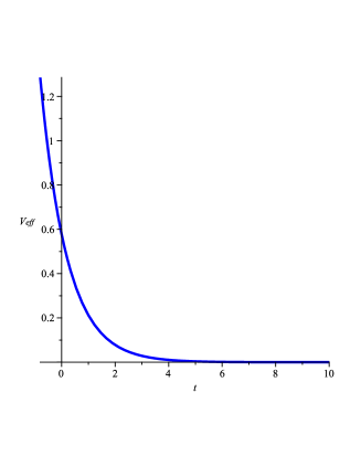
Figure 1: The time-dependent potential for a freely falling particle in de Sitter space-time

2.2 the geodesics

To derive a relation between the coordinate time and the spatial coordinates in (7), we use the geodesic equations:

$$\frac{d^{2}X^{\mu}}{d\lambda^{2}}+\Gamma^{\mu}_{\nu\rho}\frac{dX^{\nu}}{d\lambda}\frac{dX^{\rho}}{d\lambda}=0,$$ (13)

which leads to:

$$\frac{d}{d\lambda}X(\lambda)=e^{-2Ht(\lambda)},$$ (14)

$$\frac{d^{2}}{d\lambda^{2}}t(\lambda)=-\frac{3}{c^{2}}He^{-2Ht(\lambda)}.$$ (15)

The test particle’s velocity can be derived using (14) and (15) as follows [1]:

$$v=\frac{ce^{-Ht}}{\sqrt{3+e^{2Ht}\Big{(}-3+\frac{c^{2}}{v_{0}^{2}}\Big{)}}}.$$ (16)

It is easy to show that the following constraint is imposed on the initial velocity $v_{0}$:

$$v_{0}<\frac{c}{\sqrt{3(1-e^{-2Ht})}}.$$

Therefore we can obtain the relation between the coordinate time and the spatial coordinates as:

$$X(t)=\frac{c}{3H}\Big{(}\frac{c}{v_{0}}-e^{-Ht}\sqrt{3+(-3+\frac{c^{2}}{v_{0}^{2}})e^{2Ht}}\,\,\Big{)}.$$ (17)

In the next section we introduce the radiation reaction and use it to illustrate the effects of the resultant force, on particle’s trajectory.

3 Radiation Reaction

Now we present a brief review on the radiation reaction. The radiation reaction provides a recoiling force which is given by [9]:

$$F_{re}^{\mu}=\frac{2}{3}\frac{q^{2}}{c^{3}}\ddot{v}^{\mu}+\frac{2}{3}\frac{q^{2}}{c^{3}}v^{\mu}\dot{v}^{\lambda}\dot{v}_{\lambda},$$ (18)

where $v$ represents the test particle’s velocity. The Lorentz-Dirac equation which relates the particle’s motion and the external force is given by:

$$ma^{\mu}=F^{\mu}_{ext}+F^{\mu}_{re},$$ (19)

in which $a^{\mu}$ is the 4-acceleration. Considering $\frac{q^{2}}{mc^{3}}$ to be a small valued quantity and using (18) one obtains [3, 10, 11]:

$$ma^{\mu}=F_{ext}^{\mu}+\frac{2}{3}\frac{q^{2}}{c^{3}m}\Big{(}\delta_{\lambda}^{\mu}+v^{\mu}v_{\lambda}\Big{)}\partial_{\gamma}F^{\lambda}_{ext}v^{\gamma},$$ (20)

In non-relativistic limit (20) turns to [3, 11]:

$$ma=F_{ext}+\frac{2}{3}\frac{q^{2}}{mc^{3}}\dot{F}_{ext}.$$ (21)

The reader can find such relations in curved space in [12, 13].

We can rewrite (21) as $F_{total}\equiv ma$ for which we consider $F_{re}=\frac{2}{3}\frac{q^{2}}{c^{3}}\ddot{v}$. For the radiation reaction recoiling force, one can write [1]:

$$F_{re}=\sum^{\infty}_{n=1}\alpha^{n}(\frac{d^{n}}{dt^{n}})F_{ext},$$ (22)

in which $\alpha\equiv\frac{2}{3}\frac{q^{2}}{mc^{3}}.$ for small values for $\frac{q^{2}}{mc^{3}}$ we get:

$$F_{total}=\sum^{\infty}_{n=0}\alpha^{n}(\frac{d^{n}}{dt^{n}})F_{ext}.$$ (23)

In non-relativistic limits, where $v_{0}\ll c$, equation (17) leads to:

$$X(t)=\frac{v_{0}}{2H}\Big{(}1-e^{-2Ht}\Big{)}.$$ (24)

Therefore, the external force in this limit, turns to:

$$F_{ext}=m\ddot{X}(t)=-2mHv_{0}e^{-2Ht}.$$ (25)

Using (25) in (23) we obtain [1]:

$$X(t)=\frac{v_{0}}{(2H)(1+2H\alpha)}\Big{(}1-e^{-2Ht}\Big{)}.$$ (26)

This is the general equation which relates $X$ to coordinate time $t$.

4 Lagrangian Formalism

The external force in (25), provides an external momentum which is being imposed on the test particle:

$$P_{ext}=\int F_{ext}dt=mv_{0}e^{-2Ht}.$$ (27)

This momentum is a source for the kinetic energy of the test particle. We have:

$$K_{ext}=\frac{P^{2}_{ext}}{2m}=\frac{1}{2}mv_{0}^{2}e^{-4Ht}.$$ (28)

Now let us construct a Lagrangian like:

$$\mathcal{L}=K_{ext}-V_{eff},$$ (29)

in which $V_{eff}$ has been defined in (12). In de Sitter flat metric (7), this Lagrangian is a function like:

$$\mathcal{L}\equiv\mathcal{L}(t,X_{1},X_{2},X_{3},\dot{t},\dot{X}_{1},\dot{X}_{2},\dot{X}_{3}).$$ (30)

Here the dot stands for differentiation with respect to affine parameter $\lambda$ in geodesic motion. Using the metric (7) with $c=1$ yields:

$$\mathcal{L}=\frac{1}{2}\,m{{v_{0}}}^{2}{{e}^{-4\,H{t}}}-\frac{1}{3}\,m\sqrt{3}{{e}^{-H{t}}}.$$ (31)

Since we take the geometrical units ($c=1$), we have $d\lambda=d\tau$, where $\tau$ is the proper time. For indistinguishable spatial coordinates, the action in this space time, is defined by [14]:

$$S=\int\mathcal{L}(t,X,\dot{t},\dot{X})d\tau,$$ (32)

Varying this action, we can obtain the Euler-Lagrange equation of motion in de Sitter spacetime:

$$\frac{\partial\mathcal{L}}{\partial X^{i}}-\frac{d}{d\tau}\Big{(}\frac{\partial\mathcal{L}}{\partial\dot{X}^{i}}\Big{)}=0.$$ (33)

Since the metric contains only time-dependent expressions, therefore only one equation will come out from (33):

$$6\,{{v_{0}}}^{2}{{e}^{-4\,Ht\left(\tau\right)}}-\sqrt{3}{{e}^{-Ht\left(\tau\right)}}=0.$$ (34)

As we can see, the mass $m$ has no contribution in time-dependent equation. This leads to derive the following expression for $t$:

$$t(\tau)=\frac{\Big{(}2\ln(2v_{0}^{2})+\ln(3)\Big{)}}{6H}$$ (35)

4.1 shapes of the trajectory

Now we can illustrate the coordinate behaviors. First, let us concern about the coordinate time $t$, which has been shown that it has a logarithmic behavior with respect to initial velocity $v_{0}$. Using equation (35), we can plot the test particles trajectory, which is shown in Figure 2.

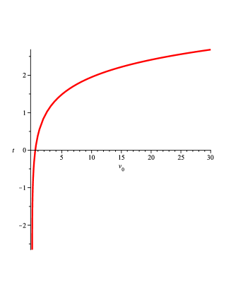
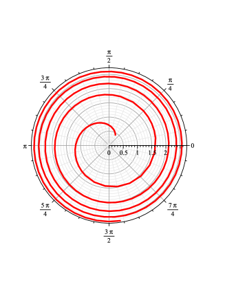
a) b)

Figure 2: a) The behavior of coordinate time with respect to initial velocity. b) The spiral behavior of time, with respect to initial velocity.

We can find out that this behavior, construct a spiral with a varying interior radius.

Another type of illustrations, is to plot the spatial coordinate $X$, with respect to coordinate time $t$. To do this, we use the the general relation (26), which includes the effects of the radiation reaction on particle’s trajectory. Figure 3 shows the so called behavior.

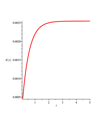
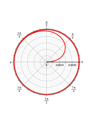
a) b)

Figure 3: a) The behavior of spatial coordinates $X$ with respect to coordinate time $t$. b) The shape of the test particle’s trajectory, in non-relativistic limit.

According to Figures 2 and 3, we will see that how the effects of radiation reaction, can make the trajectories unstable, and also causes a drop on the canter of potential.

5 Conclusion

It seems that the Liénard - Wiechert retarded potentials are not completely sufficient when the trajectories for charged particles are considered in curved spacetimes [15]. In this article, we firstly reviewed the radiation reaction, caused by particle’s radiation and derived some expressions, relating the spatial coordinates to coordinate time, in a de Sitter spacetime. Afterwards, by using a Lagrangian formalism, we derived another expression for the coordinate time, with respect to the proper time. Using these relations, we finally plotted the shapes of the trajectories, for an accelerated charged object, while falling freely in de Sitter spacetime.

Acknowledgements This work was supported under a research grant by Payame Noor University.

References

- [1] M. Fathi M. Tanhayi-Ahari M.R. Tanhayi F. Tavakoli, Radiation Effects on Geodesics in de Sitter Space: A Classical Approach, Int. J. Theor. Phys. (2012) 51:1938-1945.
-
[2]
M. Abraham and R. Becker, Theorie der Electrizität, Vol. II, (Springer, Leipzig,
1933).
H. A. Lorentz, Theory of electrons, (Dover, New York, 1952). - [3] F. Rohrlich, The dynamics of a charged sphere and the electron. Am. J. Phys 65 (11) p. 1051 (1997).
- [4] Qingming Cheng, de Sitter space, in Hazewinkel, Michiel, Encyclopaedia of Mathematics, Springer (2001), ISBN 978-1556080104.
- [5] M.R. Tanhayi, M. Fathi, M.V. Takook, Observable quantities in Weyl gravity, Mod. Phys. Lett. A, Vol. 26, No. 32 (2011) 2403-2410.
- [6] F. Payandeh, M. Fathi, Spherical Solutions due to the Exterior Geometry of a Charged Weyl Black Hole, Int. J. Theor. Phys. (2012) 51:2227-2236.
- [7] M. V. Takook, Ph.D. thesis, Universit Paris P.M. Curie (Paris 6) (1997).
- [8] C.W. Misner, K.S. Thorne and J.A. Wheeler, Gravitation, Freeman (1973).
- [9] F. Rohrlich, Am. J. Phys. 68, 12 (2000).
- [10] D. V. Gal tsov, P. Spirin, Grav. Cosmol. 13241-252, (2007).
- [11] L. D. Landau and E. D. Lifshitz, The classical Theory Of Fields, Pergamon Peress, Fourth English eddition (1975).
- [12] Dmitri Gal’tsov, Radiation reaction and energy-momentum conservation, ”Mass and Motion in General Relativity”, eds. L. Blanchet, A. Spallicci and B. Whiting, Springer Series: Fundamental Theories of Physics, Vol. 162, pp. 367-393, 2011.
- [13] M.J. Pfenning, E. Poisson, Scalar, electromagnetic, and gravitational self-forces in weakly curved spacetimes, Phys.Rev.D65:084001,2002.
- [14] Greiner W. Classical Mechanics: Sytem of Particles and Hamiltonian Dynamics. Springer-Verlag, New York, Inc., (2003).
- [15] E. Poisson, Constructing the self-force, arXiv:0909.2994v1.
- [16] S. N. Lyle, Self-Force and Inertia: Old Light on New Ideas, Lect. Notes Phys. 796 (Springer, Berlin Heidelberg 2010), DOI 10.1007/978-3-642-04785-5.