Nucleon Electromagnetic Form Factors
in the Timelike Region
Abstract
The electromagnetic form factors of the proton and the neutron in the timelike region are reviewed. In view of the forthcoming experimental projects devoted to investigate these observables, we present the current status of the field and we emphasize the relevant role, that accurate measurements, refined phenomenological analyses, as well as microscopic models will play with the goal of achieving deeper insights into the structure of the nucleon and its inner dynamics.
Keywords: Timelike form factors, Nucleon Targets, Experimental extraction, Dispersion Relations, Constituent Quark Models
1 Introduction
The investigation of the nucleon structure through electromagnetic (em) probes has played a central role in our present understanding of strong interactions. In particular, the measurements of em nucleon form factors (FF’s) in the spacelike (SL) region, which started with the pioneering work of Hofstadter [1], have given the indisputable evidence of the non-elementary nature of the proton. The possibility, offered by SL photons, of achieving an accurate description of the three-dimensional structure of the nucleon has motivated many and successful experimental efforts, which resulted in an accurate data base of the SL nucleon FF’s (see Ref. [2] for a list of recent reviews). With the advent of a new experimental technique – the so-called polarization-transfer method – a striking fall-off of the proton electric FF relative to the magnetic one, which largely follows a dipole behavior, has been discovered. This relatively recent achievement impressively demonstrates the relevance of the polarization degrees of freedom in the studies of the nucleon structure.
The transition to the timelike (TL) region, widening in such a way the investigation of the nucleon FF’s, opens unique possibilities for studying peculiar features of the nucleon state. In particular, in the TL region, one can exploit the hadronic components of the virtual photon state, that become physical, according to the proper energy thresholds. A very popular model of those hadronic components is the vector meson dominance model (see Ref. [3] for a recent review), that allows i) to develop a simple picture of the production mechanism of a physical hadron-antihadron pair, and ii) to accurately identify quantities, which are containing relevant details on the nucleon/antinucleon states. The information accessed in the TL region could appear less intuitive than the electric and magnetic distribution densities of the nucleon, but indeed they play a relevant role for shedding light on the long-range behavior of the strong interactions. TL FF’s are indeed more sensitive to the discrete hadron spectrum (given the pole structure that occurs) and to the presence of many transition amplitudes of physical processes. For instance, though the SL nucleon FF’s can be described by models, that take into account only few vector mesons, the pole pattern shown by the experimental TL FF’s cannot be reproduced without considering all the relevant vector mesons. To better understand the appealing feature of the TL region, let us go back to the fifties, when the theoretical studies on this issue began. In particular, in a paper by Federbush, Goldberger and Treiman [4], it was pointed out that a bridge can be established between the studies of the nucleon em FF’s and the transition amplitudes of physical processes, like em decays of vector mesons (VM’s) as well as the production of hadronic states with well-defined quantum numbers. This link was found through the dispersion relations that allow to express the FF’s in terms of an integral over their imaginary parts, that are non-vanishing only in the TL region. At that time, the mesonic and nucleonic degrees of freedom were the relevant ones in the field of the strong interactions, and therefore the mentioned em VM decays and hadronic transition amplitudes were considered as the relevant inputs for a phenomenological analysis. Our modern paradigm of strong interactions, Quantum ChromoDynamics (QCD), allows us to understand those physical quantities, through a microscopical description in terms of quark and gluon degrees of freedom. It should be noticed that microscopic models could represent an effective tool for evaluating the above mentioned quantities (see, e.g., the analyses in Refs. [5, 6, 7]), since Lattice QCD is greatly challenged in the TL region, differently from the SL case where electric and magnetic density distributions begin to be addressed [8].
Summarizing what has been illustrated above, it is clear that a measurement of the imaginary part of the TL nucleon FF’s, that can be achieved by exploiting the polarization degrees of freedom, is highly desirable, with a final goal of constructing a more detailed database of the nucleon FF’s, that does contain not only information on the electric and magnetic distribution densities, but also on other physical hadronic processes.
At present, the experimental knowledge of the TL nucleon FF’s unfortunately does not yet allow to achieve this goal. Compared to the SL sector, where precision measurements of FF’s have been achieved on the percent level, the data base of TL FF’s is rather scarce. Recent measurements of the BaBar collaboration [9] have somewhat improved the knowledge of the proton FF. The BaBar result concerning the ratio of the electric to the magnetic FF is however still largely limited by statistical uncertainties, and it is furthermore in conflict with a previous measurement at LEAR [10]. This only demonstrates the need for a new generation of high-precision measurements of the em FF of the proton and neutron. Indeed, new facilities at Novosibirsk, Beijing, and FAIR/Darmstadt recently came into operation or are about to start in the coming years. From these facilities we can expect significantly improved results.
The aim of the work is therefore to give an updated (maybe not complete) view to the present status of both the experimental and theoretical investigations in the field. Moreover, we hope that this review could represent an opportunity, allowing to share the common expertise, and to compare the different experimental as well as theoretical techniques, which have been worked out in the past. But, after all, the main goal is to show the wealth of information which is provided by the TL nucleon FF’s for understanding in depth the non-perturbative regime of QCD. In view of this, we will emphasize that only measurements of the relative phases will fully determine the nucleon FF’s in the TL region, so that the maximal phenomenological knowledge can be reached. Therefore, this review appears to be timely, given the near- and mid-term future experimental programs.
The review is organized as follows. Sect. 2 is devoted to the experimental studies, in particular in Subsect. 2.1 an overview of the facilities as well as the experimental techniques is given. In Subsect. 2.2, the present experimental data base is presented, and in Subsect. 2.3 the future facilities and perspectives are discussed. In Sect. 3 we present the theoretical background. We start in Subsect. 3.1 with a brief review of the SL em FF’s; in Subsect. 3.2 the general formalism for investigating the TL nucleon FF’s is presented. It follows in Subsect. 3.3 a discussion of the threshold energy region; in Subsect. 3.4 the path how to obtain the dispersion relations between the real and the imaginary part of the nucleon FF’s is shown; in Subsects. 3.5 - 3.9, several theoretical approaches are finally reviewed. In Sect. 4 some conclusions are drawn and future perspectives are presented.
2 The experimental investigation of TL nucleon form factors
In the year 1972 the first measurement of a TL nucleon FF was performed at the collider ADONE in Frascati using the process [11]. This historically first result was obtained with an optical spark chamber setup at a center-of-mass energy (c.m. energy) of GeV/c. In the following years a series of measurement campaigns were performed at the electron-positron colliders ADONE with the FENICE experiment [12, 13], as well as at the Orsay colliding beam facility (DCI) with the detectors DM1 [14] and DM2 [15, 16]. The em FF of the proton was explored by these facilities from nearly production threshold (, where is the mass of the proton) up to c.m. energies of GeV/c. Precision measurements were also obtained with the BES-II experiment [17] at BEPC, and with CLEO [18] at CESR. The information concerning the TL FF of the neutron is especially scarce, with only the FENICE experiment so far having been able to perform this measurement, cf. Refs. [13, 19].
First attempts to measure the proton FF using the inverse reaction date back to the mid 1960’s. Indeed, first upper limits stem from antiproton beam experiments at BNL [20] and CERN [21]. The discovery of this reaction was finally possible using an antiproton beam at PS/CERN in 1976 [22]. Antiproton experiments were later continued with great success at LEAR/CERN with the PS170 experiment [10, 23, 24] and at FNAL [25, 26, 27].
In the experiments mentioned above, em FF’s have been measured using the so-called energy scan method, i.e. by systematically varying the c.m. energy of the collider. Around the beginning of the 21st century, particle factories came into operation, such as the B-factory PEP-II at SLAC, which was operated at a c.m. energy corresponding to the mass of the (4S) resonance of GeV. It was realized that the use of events with photon radiation from the initial state (ISR) appears to be a copious source of hadronic final states with invariant masses below the actual c.m. energy of the collider. Competitive results of the proton [9] as well as of the , , and FF’s [28] have been achieved at the BaBar experiment in the course of the years. The BaBar data set does not only feature the best statistical and systematic precision achieved to date, but it is also spanning the entire energy range of interest from threshold up to GeV. The BELLE collaboration at the Japanese B-factory project KEK-B has been using the ISR-technique in the charmonium energy region and has measured the process [29].
2.1 Experimental techniques and facilities
We report in this Subsect. on the various experimental techniques (see also Fig. (1)) and facilities, as outlined above. A compilation of the experimental results follows in Subsect. 2.2. An outlook concerning future perspectives in the field will finally be discussed in Subsect. 2.3.
2.1.1 Energy scan experiments in annihilation
The standard technique for measurements of hadron production in electron-positron annihilation is the so-called energy scan, in which the c.m. energy of the collider, , is varied systematically, see Fig. (1,a). At each energy point a measurement of the associated cross section is carried out. In the case of nucleon pair production, , the associated FF’s are related to the total cross section in one-photon approximation (see Subsect. 3.2 for a more detailed discussion) according to:
| (1) |
where is the electromagnetic fine structure constant, the nucleon velocity, is the s-wave Sommerfeld-Gamow factor, that takes into account the Coulomb effects at threshold (see Eq. (30) and below for more details), and the nucleon mass. and are the electric and magnetic Sachs FF’s, respectively, which depend on the square four-momentum transfer of the virtual photon, . Neglecting radiative corrections, the four-momentum transfer and the c.m. energy of the collider are identical, cf. Eq. (1):
In none of the energy scan experiments performed so far, the Sachs FF’s could be disentangled by means of a measurement of the differential cross section (see below), and the data are therefore shown in terms of an effective FF defined as follows:
| (2) |
where the rightmost-hand side shows the relation with the Sachs FF’s in one-photon approximation.
We want to stress that any experimental measurement of is independent of any assumption on or 111 In literature, it is often stated that the experimental value of is obtained assuming , which is incorrect., and it quantitatively indicates how much the experimental cross section differs from a point-like one (cf. Eq. (35)). Summarizing, the cross section can be written as a product of a point-like cross section and , that contains information on the transition amplitude from a virtual photon state to a state (i.e, in a naive picture, , through all the allowed paths, see also Subsect. 3.2).
The cross section itself is obtained by measuring the total number of nucleon pairs, , after background subtraction () and by normalizing to the total integrated luminosity (). Since detectors cannot cover the full solid angle, the geometrical acceptance () and detection efficiencies (), as well as radiative corrections () need to be considered:
| (3) |
Table (1) shows a compilation of nucleon FF measurements, which have been obtained via the energy scan technique. While the channel has been measured by several experiments (Refs. [11, 12, 13, 14, 15, 16]), data on the final state so far exist only from FENICE [12, 13]. The experiment DM2 also measured at one single energy point the process [16]. As can be seen from Table (1), the energy range from production threshold up to GeV has been covered via energy scan experiments. Typical energy steps in the individual scanning campaigns vary from MeV – in the case of the Frascati and Orsay experiments – up to MeV in the case of BEPC [17]. At 3.67 GeV, one single energy point has been published by CLEO at Cornell [18]. With integrated luminosities well below pb-1 per scan point (in almost all cases) and given the small cross section for the process , the collected statistics typically was very low. Even close to threshold, where the cross section for baryon-pair production is highest (but still below nb), the statistics per scan point did not exceed events. We briefly discuss in the following the methodology used at the experiments DM1 / DM2 (Orsay), the FENICE experiment (Frascati), and the BES experiment (Beijing).

| Exp. | Reaction |
|
|
Range [GeV] |
|
Events | Ref. | ||||||
|---|---|---|---|---|---|---|---|---|---|---|---|---|---|
| DM1 | 1979 | 4 | 0.4 | [14] | |||||||||
| DM2 | 1983 | 6 | 0.5 | [15] | |||||||||
| DM2 | 1990 | 1 | 2.4 | 0.2 | 7 | [16] | |||||||
| DM2 | 1990 | 1 | 2.4 | 0.2 | 4 | [16] | |||||||
| ADONE 73 | 1973 | 1 | 2.1 | 0.2 | 25 | [11] | |||||||
| FENICE | 1993 | 2 | 0.1 | 27 | [19] | ||||||||
| FENICE | 1993 | 1 | 2.1 | 0.1 | 28 | [19] | |||||||
| FENICE | 1994 | 4 | 0.3 | 70 | [12] | ||||||||
| FENICE | 1998 | 5 | 0.4 | 74 | [13] | ||||||||
| FENICE | 1998 | 1 | 2.1 | 0.1 | 7 | [13] | |||||||
| BES-II | 2005 | 10 | 5 | 80 | [17] | ||||||||
| CLEO | 2005 | 1 | 3.671 | 21 | 16 | [18] |
-
•
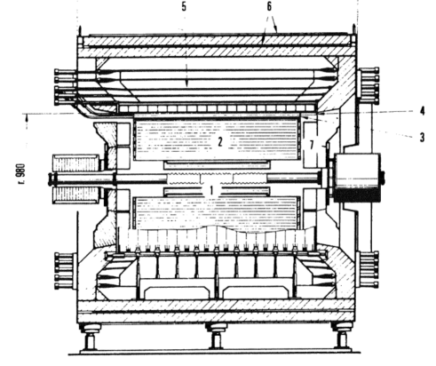
At the Orsay colliding beam facility DCI the nucleon FF measurements were performed with the detectors DM1 and DM2. A sketch of the DM2 detector is shown in Fig. (3). It already resembles the typical structure of modern collider experiments with large geometrical acceptance. DM2 consisted of several layers of cylindrical multiwire proportional chambers (MWPCs) inside a magnetic field of solenoidal shape. In two scan campaigns (four and six scanning points each) the energy range between GeV and GeV could be covered; in total, approximately events were selected.
-
•
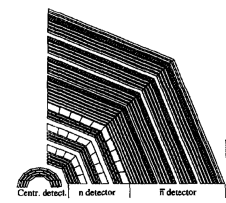
The non-magnetic FENICE detector (cf. Fig. (3)) at the ADONE collider was designed with the primary goal to measure the neutron FF. The main components of the experiments were Limited-Streamer-Tube (LST) modules as tracking devices, scintillation counters as triggering and timing devices and thin iron plates as distributed converters for the antineutron detection [13]. The specific signature of an antineutron annihilation ’star’ together with the long TOF between production and annihilation, were mainly used to detect anti-neutrons. No dedicated neutron detection was performed due to the relatively low neutron detection efficiency. The neutron FF has been measured from values close to threshold up to GeV. A precise determination of the proton FF in the same energy range has been possible as well.
-
•
From an energy scan (10 scanning points) of the BEPC collider in the range GeV/c GeV/c, the BES-II experiment could extract the proton FF, extending significantly the energy range covered before at Frascati and Orsay. BES-II was a typical multiple-purpose detector with large acceptance, consisting of a vertex chamber, a large cylindrical drift chamber, a TOF system as well as a photon detector setup. The whole apparatus was embedded in a solenoidal coil. The precision of the proton FF measurement at BEPC was mostly limited by statistics. In total, events have been detected. The systematic uncertainty was close to in all scan points.
2.1.2 annihilation
Starting in the 1960’s, antiproton beams became available, which were also used to search for the process , see Fig. (1,b). The antiproton beam is scattered on a hydrogen target in a fixed-target configuration. The momentum transfer squared, , of the em FF in this case is accessible by measuring the invariant mass of the lepton pair, or, alternatively, it is calculated for a given antiproton beam momentum assuming the target protons to be at rest. First upper limits for the TL proton FF have indeed been obtained at relatively high energies at BNL [20] and CERN [21] in ranges between (GeV/c)2 and (GeV/c)2. For historical reasons we report FF results from experiments as a function of the c.m. energy of the collider, , while results from annihilation experiments are quoted as a function of .
In the year 1976 – 3 years after the first Frascati measurement of a TL nucleon FF in scattering – the first positive result was achieved by the Mulhouse-Strasbourg-Torino collaboration [22] with an antiproton beam at PS/CERN. In total, candidate events, which were produced by stopped antiprotons in a liquid hydrogen target, as well as additional events, in which the annihilation process took place ’in-flight’, had been recorded. The experimental setup consisted of several optical spark chambers surrounded by an array of scintillators. Due to the low antiproton beam momenta, for the first time the proton FF could be measured at values almost at the production threshold.
Indeed, annihilation experiments allow for a complementary access to the TL proton FF. Differently to colliders, the production threshold does not feature a limited phase space for the outgoing particles, and furthermore, one does not have to deal with the experimental issues related to low-momenta protons in the target region. On the other hand, no baryon FF’s different from protons can be accessed in annihilation experiments, and the rejection of background with hadronic final states is an experimental challenge.
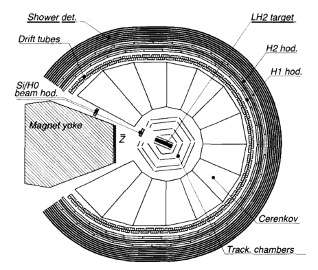
With the advent of a dedicated storage ring for low-momenta antiprotons at CERN, the LEAR ring, significant progress could be achieved also for measurements of the TL proton FF. A dedicated experiment PS170 was able extract the FF at different values from threshold up to (GeV/c)2 [10, 23, 24]. Not only the beam intensity was increased with respect to the previous CERN experiment, but also the instrumentation was more advanced. The PS170 detector consisted of several layers of MWPCs as tracking detectors, Cerenkov detectors, and hodoscopes inside a T magnetic field. It was possible to separate signal events from two-body processes involving hadrons. Fig. (4) shows a sketch of the detector. In a sophisticated analysis, the yield of the final state was normalized to the yield of the two-body hadronic reactions and . The cross section for the process was then computed using the known ratio of hadronic two-body final states to the total annihilation cross section, cf. Ref.[10] for more details.
For antiprotons stopped in the liquid hydrogen target – i.e. for events very close to threshold – a large statistics of almost events could be collected, exceeding the previously available statistics by more than one order of magnitude. The extracted FF was however limited by systematic uncertainties. Due to the fact that the stopped antiproton is forming a atom, only the configuration with quantum numbers is relevant for the em FF. Hence, the fraction of quantum states, as well as the ratio of the spin singlet to triplet probabilities need to be known. Overall, an uncertainty of approximately % was achieved at threshold.
The large angular acceptance together with the relatively high statistics did also allow for a first measurement of the differential cross section using ’in-flight’ events. In one-photon approximation, this differential cross section is given by
| (4) |
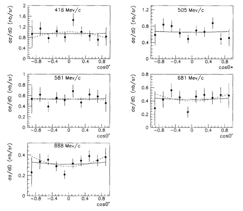
where is the angle between the proton and the beam direction in the c.m. system, and the antiproton momentum in the CM system ( see also Eq. (26). From the measurement of the differential cross section (cf. Fig. (5)) and using Eq. (4), the ratio could be extracted. The experiment PS170 has measured this ratio for five different values, although with relatively large statistical and systematic uncertainties of %. The result for the ratio will be presented in the next Subsect..
In the 1990’s and at the beginning of the new century, measurements of the TL proton FF have been obtained also at FNAL, where a high-intensity, stochastically-cooled antiproton beam used to be in operation. Using a hydrogen gas target, the experiments E761 and E835 covered the high- range between (GeV/c)2 and (GeV/c)2. Those were the highest momentum transfers achieved at the time, exceeding the measurements at BES-II in electron-positron annihilation. At the highest energy point, (GeV/c)2, only an upper limit could be established. In contrast to the low-momenta antiproton experiments performed at LEAR, at FNAL the cross section measurement could be normalized to the integrated luminosity, which was monitored by a dedicated monitoring system using elastically scattered antiprotons as a reference process. The cross section is determined using Eq. (2) – with the only difference that a different kinematic flux factor has to be considered – , and Eq. (3) with to be replaced with , where corresponds to the number of events.
Table (2) shows a summary of all results from annihilation experiments for extracting TL nucleon FF’s.
2.1.3 Initial State Radiation
Around the year 2000, a new generation of high-luminosity electron-positron colliders came into operation, which were explicitly designed to operate at fixed c.m. energies, , corresponding to the mass of either the -resonance – in the case of the -factory DANE in Frascati – or the mass of the -resonance – in the case of the B-factories PEP-II at SLAC and KEK-B in Tsukuba. As those resonances provide the highest statistics for coherent production of pairs of K- and B-mesons, the main physics motivation for the above mentioned facilities was the measurement of CP-violation in K- and B-meson systems.
Energy scans over wide energy ranges were technically not possible at the first generation - and B-factories. It was realized, however (see Refs. [31, 32, 33]), that the very high luminosities did allow for a complementary approach to the standard energy scan. Events with photon radiation from the initial state (ISR), cf. Fig. (1,c), lead to a reduction of the invariant mass of the virtual photon, , and hence allow for a measurement of the hadronic FF’s at energies below . By measuring the invariant mass of the hadronic system, , the entire energy range below the c.m. energy of the collider becomes accessible: . By neglecting effects of final state radiation (FSR), the following relation holds for the four-momentum transfer :
Comprehensive reviews of the ISR method, which is also called Radiative Return technique, can be found in Refs. [34] and [35]. The method was both used for measurements of hadronic reactions with mesons in the final state, as for the measurement of baryon pair production:
The BaBar experiment at the SLAC B-factory PEP-II has measured the TL proton FF below GeV, and has furthermore investigated the following three hyperon final states: , , and . Before BaBar no experiment had the sensitivity to measure the latter two channels. The full BaBar data set comprises an integrated luminosity of fb-1, collected between 1999 and 2008. BaBar results of mesonic final states, i.e. of final states containing two pions, three pions, four pions etc. are very valuable input for evaluating the hadronic contributions to and the running fine structure constant . Notably, a measurement of the TL pion FF from threshold up to GeV with % precision in the peak region was achieved [36]. Furthermore, a series of interesting structures have been observed in the mass spectra, e.g. a destructive interference effect in the final states [37] at an energy being very close to the threshold. Among the major results of the ISR programme at BaBar, we want to mention also the discoveries of the [38] and [39] resonances.

On the theoretical side, the ISR process was calculated within QED up to Next-to-Leading Order (NLO) and the probability for ISR photon emission can be expressed by means of a radiator function [32, 33, 40]. Notice that high energies of the ISR photon correspond to small values of . Neglecting again effects of FSR (see Ref. [41] concerning this issue), i.e. assuming , the non-radiative cross section can be extracted from the measured radiative cross section by using this radiator function:
| (5) |
The calculation of the radiator function is usually performed with the Monte Carlo method; a dedicated Monte Carlo generator for ISR processes has been developed within the PHOKHARA package, which simulates a large number of hadronic reactions, including also the baryonic final states [42] , , and [43]. PHOKHARA simulates the full NLO-ISR radiative corrections [44]. Within the BaBar collaboration, besides PHOKHARA, also the AFKQED Monte Carlo package has been developed, which is simulating FSR corrections by means of PHOTOS [45] and which uses the structure function approach for higher order ISR corrections. The AFKQED generator is based on an early version of PHOKHARA, called EVA, cf. Refs. [32, 46].
Due to the specific energy dependence of the ISR photon, the radiator function decreases steeply with . In Fig. (6), the so-called ISR luminosity is shown, which is the product of the radiator function times the integrated luminosity: . The specific values for BaBar ( GeV, fb-1) have been used in Fig. (6). The geometrical acceptance () and detection efficiency () have been considered as well ().
The ISR luminosity allows to compare the number of ISR events produced for a given final state and for a given mass value with the direct production in an energy scan; depends of course on the chosen bin size and decreases with finer binning. At the production threshold, the ISR luminosity is found to be pb-1 (assuming a bin width of MeV/c2) and therefore exceeds the statistics collected at ADONE and DCI. Apart from the large statistics, the ISR method offers some additional advantages over conventional energy scan measurements:


-
•
A very valuable feature is the fact that in one single experiment the entire energy range of interest can be covered. This avoids the notorious problems associated with combinations of different data sets, which are usually having different normalization uncertainties. At BaBar, the proton FF could be measured over a very wide mass range from production threshold up to GeV/c, which has never been possible before and which exceeds the energy range covered by BES-II and the FNAL experiments.
-
•
In the baryon FF measurements performed at BaBar, the ISR photon has been tagged in the em calorimeter (EMC) at relatively large polar angles. Events with small angle ISR photons, which a priori have a much higher cross section, lead to an event signature, in which the hadronic system is emitted opposite to the ISR photon. The hadronic particles are hence flying outside the detector acceptance. The lower the invariant of the hadronic system is, the higher is the probability to lose at least one of the hadronic particles in the final state. However, for the tagged photon approach this back-to-back signature has its own merits, namely it leads to the fact that the geometrical acceptance for events is very flat compared to usual energy scan experiments. This can be seen in Fig. (8), where the angular acceptance for events is shown. The almost uniform angular distribution reduces the model dependence of the cross section measurement due to the unknown ratio, which represents a major limitation in the data analysis of energy scan experiments.
-
•
Furthermore, for ISR events – differently from standard experiments – the momenta of the final state particles at threshold are non-zero. This does not only reduce the systematic effects, which are usually unavoidable when dealing with low-momenta particles, but it leads also to a flat reconstruction efficiency as a function of , which is especially important if the FF at threshold is investigated. In Fig. (8) the mass resolution as a function of the hadronic mass is shown. At low masses, the mass resolution is as small as MeV/c2. In order to improve the mass resolution and to reject background channels, a kinematic fit is usually performed.
We conclude that the ISR technique is a very competitive method for the measurement of baryon TL FF’s. Moreover, the high statistics and accuracy of the BaBar measurement of the proton FF [9] allowed a measurement of the ratio in five energy bins. Like in the case of the PS170 experiment, the angular distributions are investigated to disentangle and . However, when using the ISR technique, the existence of an additional high-energetic photon in the final state needs to be taken into account. In the BaBar analysis, the differential cross section with respect to the cosine of the angle has been fitted (cf. Fig. (9)), where is the angle between the proton in the rest frame and the momentum of the system in the rest frame (remember that PEP-II is an asymmetric collider built for CP studies in the B-meson sector). In Ref. [43] it has been suggested to use a different approach, namely to consider the proton angular distribution in the hadronic rest frame, with the z-axis aligned with the direction of the ISR photon and the y-axis in the plane determined by the beam and the photon directions.
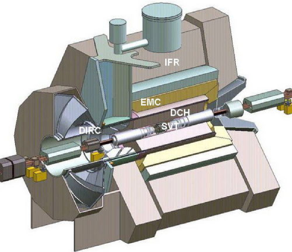
Fig. (10) shows a sketch of the BaBar detector. Charged particles are detected in the BaBar tracking system, which comprises a five-layer silicon vertex tracker (SVT) and a 40-layers cylindrical drift chamber (DCH) operating in a T solenoidal magnetic field. The momentum resolution for a GeV/c track is %. Particle identification is provided by a an internally reflected Cerenkov detector (DIRC), as well as by information from the tracking system. The energy and position of photons is measured by a CsI(Tl) em calorimeter (EMC); muons are identified by a dedicated detection system inside the iron coil (instrumented flux return, IFR). No attempts have been made at BaBar to measure the detection efficiency of neutrons inside the EMC; only the proton-antiproton final state as well as hyperon channels, which decay into protons and pions, have been investigated.
| Exp. | Reaction |
|
|
Range [GeV] |
|
Events | Ref. | ||||||
|---|---|---|---|---|---|---|---|---|---|---|---|---|---|
| BaBar | 2005 | 47 | 232 | 4025 | [9] | ||||||||
| BaBar | 2007 | 12 | 232 | 138 | [28] | ||||||||
| BaBar | 2007 | 4 | 232 | 24 | [28] | ||||||||
| BaBar | 2007 | 5 | 232 | 18 | [28] | ||||||||
| BELLE | 2008 | 50 | 659 | not cited | [29] |
Table (3) gives a summary of the ISR measurements of TL baryon FF’s, which have been performed so far. Besides the BaBar results reported above, the BELLE experiment at the Japanese B-factory project KEK-B has investigated the process in the energy range between GeV and GeV using the ISR technique [29]. The integrated luminosity collected at BELLE is exceeding fb-1 and is hence twice as large as the luminosity available at BaBar. Until now, the ISR programme at BELLE has been entirely devoted to the production of charm and charmonium resonances in the mass range above GeV/c2. In the case of the analysis, a resonance at MeV/c2 and a width of MeV has indeed been found.
2.2 Experimental results
In this Subsect. the experimental results obtained in in the extraction of TL baryon FF’s are summarized. While the main focus of this review is the physics of the TL FF of the proton and of the neutron, we also present the results obtained by BaBar on hyperon FF’s. Furthermore, we discuss some phenomenological aspects related to the FF measurements. The in-depth discussion of the theoretical background follows in Sect. 3.
2.2.1 TL proton electromagnetic form factor
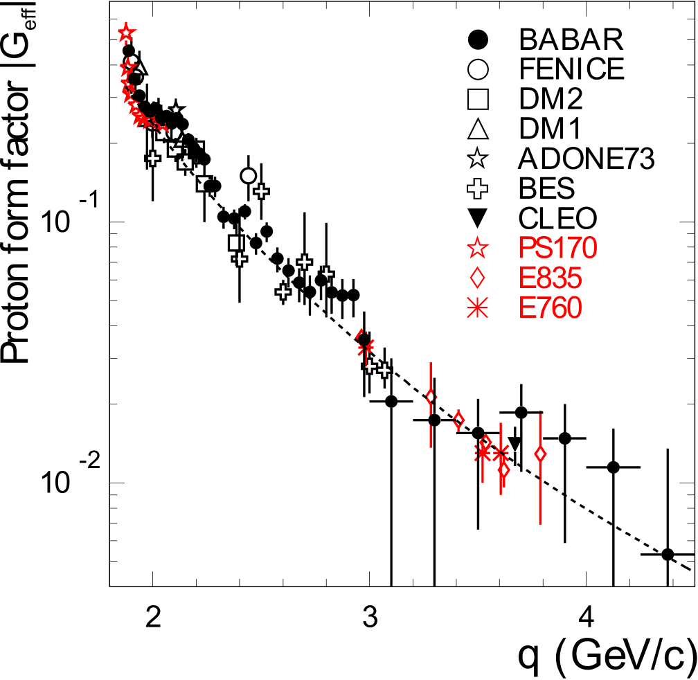
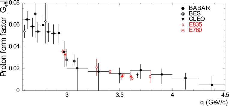
In Fig. (12) the various measurements of the cross section, performed at colliders, are summarized, see Tables (1) and (3). The energy range between the production threshold and GeV has been covered. Fig. (12) shows the effective FF for those data sets and includes in addition the results obtained via proton-antiproton annihilation at CERN and FNAL, cf. Table (2). We have omitted the older CERN results of Refs. [23, 24, 22] which are superseded by the high-statistics measurements of experiment PS170 (Ref.[10]). In general we can identify a good agreement among the different data sets. Nevertheless, the complex shape of the TL proton FF is largely not understood and has lead to many speculations. We briefly summarize the most relevant observations.
-
•
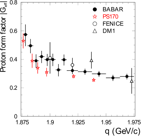
The FF shows a very steep rise toward threshold, which can be clearly identified in the two data sets of BaBar and PS170. A zoom to the threshold region is shown in Fig. 13 (linear vertical scale), in which the BaBar spectrum is plotted in a finer binning to take account of the rapid FF change. Although the BaBar and PS170 spectra seem to indicate some normalization issues, the threshold enhancement is clearly visible also in this plot. It is interesting to note that a similar behavior can be seen also in the invariant mass spectra of very different physics processes, e.g. B-decays (, ) measured at BELLE [47] and BaBar [48] as well as the decay measured at BES [49]. It has been speculated whether the threshold enhancement might be due to the existence of a hypothetical, narrow resonance with a mass just below threshold. Indeed, such a narrow bound state could give rise to a dip in the energy dependence of the cross section as a result of an interference effect with a broad resonance [50]. Several experiments had observed such a dip in the energy spectrum of the state [51] and more recently also BaBar has confirmed this observation in the and exclusive states [37]. We will discuss the physics of the threshold region in more detail in Subsect. 3.3.
-
•
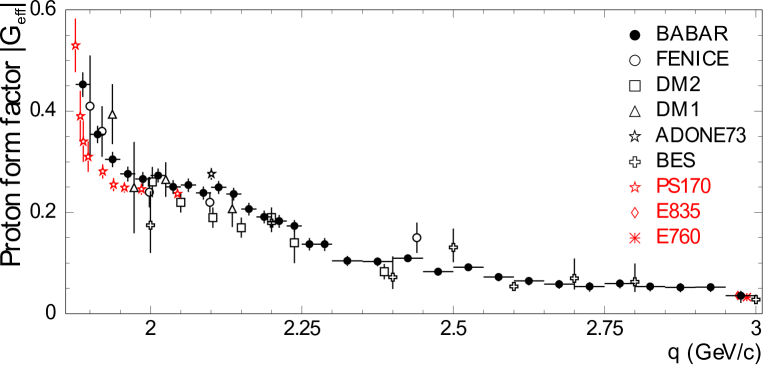
Fig. (14) shows the energy dependence of in the energy range from threshold to GeV (upper plot), and from GeV to GeV (lower plot). The events from and decays to are subtracted from the contents of the corresponding bins. Two rapid decreases of the FF and cross section near GeV and GeV are seen by BaBar. Rosner has pointed out [52] that these steps are just below the respective thresholds for and systems, respectively, and suggests an s-wave threshold effect to be responsible for these structures.
-
•
Finally, a comparison of the asymptotic behavior of the TL proton FF at high with the corresponding SL FF, measured in scattering, represents another puzzle. While perturbative QCD calculations and the application of the Phragmén-Lindelöff theorem (cf. Subsect. 3.4) predict the asymptotic values for SL and TL FF’s to be identical at high energies, the experimental investigation of this issue is confronted by the difficulties of disentangling the electric and magnetic FF in the TL region. If one assumes that the effective form factor could be an approximation of the TL magnetic form factor (cf. Eq. (2)), one finds that it is larger than the corresponding SL quantities by about a factor of two. In order to perform this comparison, one has to assume that the TL magnetic FF is positive in the asymptotic region (cf. Subsect. 3.7 for a more detailed discussion).
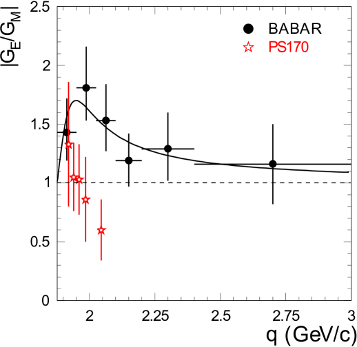
In Figs. (9)and (5) the results of BaBar [9] and PS170 [10] on the differential cross section had already been presented. We remind that according to Eq. 4 the ratio becomes accessible from the measurement of . Fig. (15) shows the results obtained by both collaborations on this ratio. The experiment PS170 has measured in five energy bins below GeV; BaBar has measured the ratio in six energy bins below GeV. While the spectrum of the PS170 experiment seems to be compatible with the assumption , the BaBar spectrum shows a relatively large deviation from for intermediate energies.
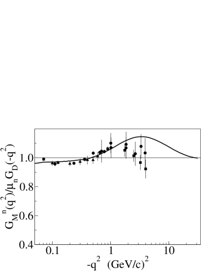
2.2.2 TL neutron electromagnetic form factor
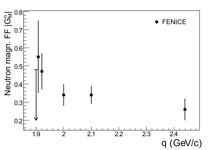
As mentioned above, only FENICE has measured so far the FF for the reaction . In addition to the usual choice of using an effective FF (cf. Eq. (2)), the FENICE collaboration has also analyzed the neutron FF by assuming in the one-photon cross-section, namely identifying the ratio
with the magnetic FF of the neutron (see also Subsect. 3.2). This was motivated by the angular distributions measured in the experiment, which were compatible with a shape, only. The data, hence, did not allow for an additional term proportional to , which would have indicated a significant contribution from the electric FF, see Eq. (4). In Fig. (16), as in Ref. [13], the data are shown in terms of the previous ratio.
Although the process is measured with very low statistics, the FF is found to be systematically higher than in the case of the proton. This effect is not understood and needs an experimental confirmation, especially since naive quark models predict the TL proton FF to be higher than the neutron one.
2.2.3 TL hyperon electromagnetic form factors
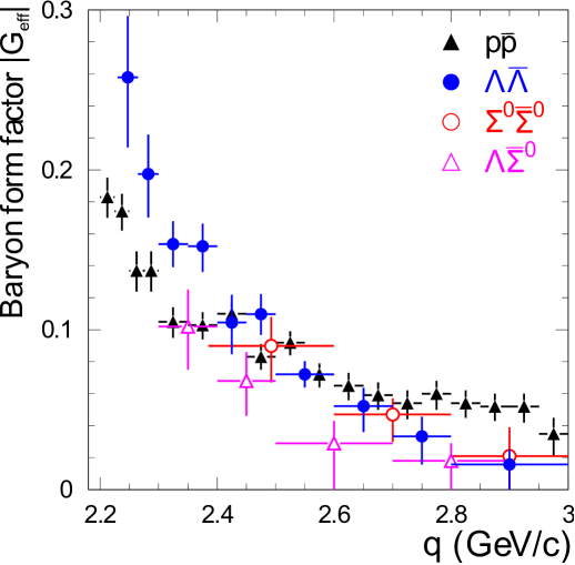
The BaBar measurements of hyperon effective FF’s are presented in Fig. 17. The results for the hyperon final states , and are shown together with the proton FF. Although, the hyperon FF’s are having significantly larger uncertainties confronted to the proton case, there is clear evidence that all measured FF’s are featuring a strong threshold enhancement. Again, this behavior is not understood.
A nonzero relative phase between the electric and magnetic FF’s and leads to a polarization of the outgoing baryons with the polarization being proportional to . The polarization can be measured in the decay using the correlation between the direction of the polarization vector and the direction of the proton from the decay. Due to the low statistics collected at BaBar, only a weak limit could be extracted for this phase: . In Ref. [28] also the ratio was investigated in two mass intervals. Again, the low statistics did only allow for measurements with large uncertainties. is found to be for the mass range GeV GeV and for GeV GeV, where is the invariant mass of the system.
2.3 Experimental outlook
At present, the knowledge of the em FF’s of the nucleon in the TL regime remains largely not understood. This statement appears obvious, given the various phenomenological puzzles mentioned above. The relevance of a better experimental data base for an improved theory prediction will be discussed in detail in Sect. 3. While experiments have been able to measure the shape of a so-called effective FF of the proton, , with a precision of a few percent at threshold, the uncertainties are much larger at higher momentum transfer. The neutron FF remains almost terra incognita. To receive a significant progress in our understanding of TL nucleon FF’s, the future experimental programme, in our opinion, should concentrate on the following aspects:
-
•
Consolidate the existing FF measurements of the proton, and obtain first precision data for the FF of the neutron (as well as for hyperons);
-
•
Obtain statistically significant results for the ratio ;
-
•
Measure the relative phase between the electric and magnetic Sachs FF’s.
Fortunately, in a world-wide effort such an experimental programme is currently pursued. All experimental techniques presented in Subsect. 2.1.1 will be used: the energy scan, the ISR technique, and the annihilation method.
Very recently the VEPP-2000 electron-positron accelerator in Novosibirsk came into operation with c.m. energies of up to GeV and with a design luminosity of cm-2s-1 at the highest beam energies. First preliminary results by the CMD-3 and SND collaborations concerning TL nucleon FF’s have already been presented at conferences [53], both for the as well as for the final states. These first results indicate that – once the design luminosity will be achieved – we can expect approximately and events produced close to threshold and the ratio to be measured with % accuracy.
Furthermore, the second generation B-factory projects in Japan and Italy [54], which will start operation in several years from now, foresee an increase of luminosity of up to two orders of magnitude compared to the first generation. The ISR method will be applied at those facilities and the statistical errors for future FF measurements will be reduced by up to an order of magnitude.
In the following, we will present in more detail two facilities for which a significant progress in the field can be expected in the near-term future, especially at intermediate and large energies, where an extraction of the ratio is of major importance. These are the BES-III experiment at Beijing and the PANDA experiment at the future FAIR facility in Darmstadt.
2.3.1 BES-III at the collider BEPC-II
The BEPC-II collider in Beijing is a next-generation -charm factory with c.m. energies corresponding to the mass of the charmonium resonances. Data taking started in 2009 with more than fb-1 of integrated luminosity having been collected since then. The world’s largest statistics of , , and decays is already available at BES-III, see Ref. [55] for a detailed summary of the physics programme. The accelerator is designed to have the highest instantaneous luminosity on the resonance. Peak luminosities of cm-2s-1 have been achieved. This corresponds to % of the design value. For lower and higher energies, the instantaneous luminosity drops by up to an order of magnitude. Since the BEPC-II accelerator (differently from the B-factories) is designed to operate not only at one single beam energy, an excellent chance for a new precision measurement of the TL nucleon FF’s over a wide energy range is given.
Such an energy scan between to GeV is indeed scheduled for the coming years. In a first campaign, the step sizes will be approximately MeV wide with a finer binning eventually at GeV and GeV, where steps in the spectrum of the proton FF have been found (cf. Fig. (14)). Based on the current performance of the accelerator, the integrated luminosities per scan point can be estimated to be between pb-1 (at GeV) and up to pb-1 (below and above the resonance). Compared to the scan performed by the predecessor experiment BES-II (Ref. [17]), this implies not only a significant increase of the number of scan points as well as of a broadening of the energy range, but also an increase in statistics of about two orders of magnitude. According to the current plannings, detected events at GeV and events at GeV will be detected. Also concerning the systematic uncertainties, which used to be below % in the case of BES-II, a major progress can be expected, given the improved detector performance. The statistical error will however still be dominating the overall precision in most of the energy range.
A determination of the em FF of the neutron seems feasible as well at BES-III. A recent measurement of the branching fraction [56] with % uncertainty has demonstrated the sensitivity of the BES-III detector for neutron and antineutron detection, which is the major issue in this analysis.
The high integrated luminosities available at BES-III, will also allow for a programme of ISR measurements of TL nucleon FF’s. Notice that the threshold region for production will only be accessible via ISR, given the fact that for technical reasons an operation of the collider below GeV is most likely impossible. Background conditions appear to be optimal for runs taken on the resonance, on which fb-1 of integrated luminosity have already been taken and for which fb-1 are expected for the coming years. A feasibility study [57] shows, that the expected statistics at BES-III will be competitive with the existing BaBar measurement. The fact that the c.m. energy of the BEPC-II collider is very close to the hadronic mass range of interest, leads to a radiator function (see Eq. (5)) which is advantageous with respect to the measurements performed at BaBar. This effect cannot be overcompensated by the higher integrated luminosities available at the B-factories. Moreover, the fact that the ISR photon at BES-III is much less energetic compared to BaBar, opens the possibility for so-called untagged measurements, in which the detection of the ISR photon is not explicitly required. Since the differential cross section for ISR events increases significantly for low-angle photons, the untagged approach offers a very high statistics at a good signal-to-background ratio 222The feasibility of untagged measurements was already proven in ISR-analyses of the TL pion FF at the KLOE experiment at DANE [58]..
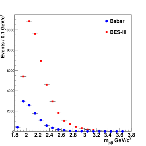
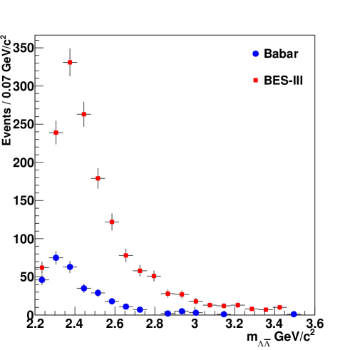
The expected BES-III statistics in terms of produced events using the ISR technique can be seen in Fig. (18) for the channel (left plot) and for the channel (right plot). An integrated luminosity of fb-1 has been assumed in these simulations. For the sake of comparison, the event yield for the BaBar case for an integrated luminosity of fb-1 is shown as well. Since the geometrical acceptances and detection efficiencies might be different between BES-III and BaBar, we only compare the number of produced events333 We remind that the fully available BaBar statistics is about a factor two larger than the one used in the published results of Refs. [9, 28] and the one assumed in Fig. (18).. In order to facilitate the detection of ISR-produced events, a dedicated tagging detector [59] has been installed in the BEPC-II beam line at very small polar angles. This tagging device is intended to detect ISR-photons at very small polar angles. The precision of the future measurement remains however to be investigated.
2.3.2 PANDA at the HESR antiproton beam at FAIR
The HESR storage ring at FAIR [60], which will start operation in 2018, will provide a high-intensity and high-resolution antiproton beam in the multi-GeV energy range. The beam will be scattered on a proton target (pellet or gas jet) within the PANDA detector, yielding luminosities of cm-2s-1 and higher. This is an improvement of an order of magnitude compared to the luminosity, which used to be available at FNAL.
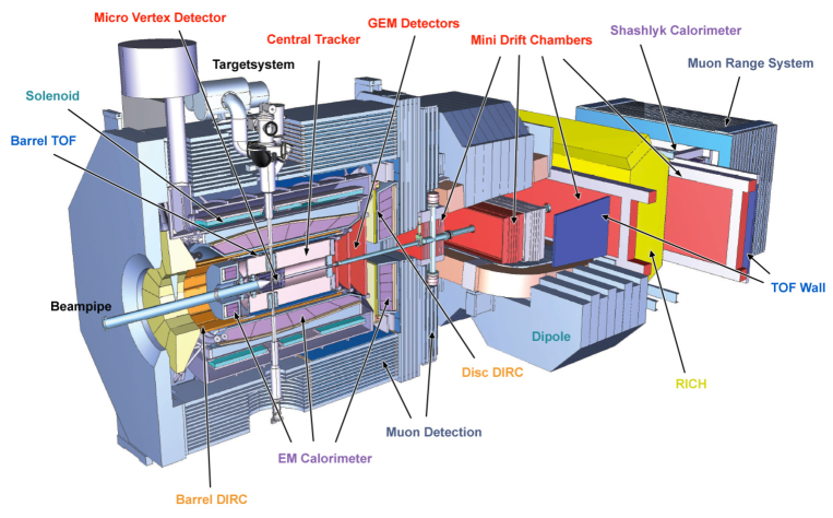
The PANDA detector, which is shown in Fig. (19), consists of a barrel as well as a forward detector. The barrel detector resembles the geometry of typical collider experiments (see e.g. Fig. (10)) with a solenoidal magnetic field. The forward spectrometer reflects the fixed target concept of the experiment and contains a dipole magnet to allow for a momentum measurement of particles scattered at small polar angles. The electromagnetic calorimeter of PANDA, the straw tube tracking system together with a dedicated DIRC Cerenkov detector setup will be of utmost relevance for a precision measurement of the process. With antiproton beam momenta between GeV/c and GeV/c available at the HESR, the em FF of the proton in the range between (GeV/c)2 and (GeV/c)2 can be accessed [61].
Detailed feasibility studies have been performed to prepare the measurement of the proton FF, cf. Ref. [62]. A serious background remains from two-body processes like and , which happen to have up to six orders of magnitude higher cross sections compared to signal events. A special effort has indeed been made to provide realistic event generators for those processes (cf. Ref. [62]). In the background process, Dalitz decays of neutral pions can be rejected by appropriate angular cuts. The background channel requires very good PID capabilities and a good understanding of their experimental efficiencies. Kinematic fits help to reject the hadronic two-body background channels as well as other background processes. Taking into account all these analysis items, and by performing realistic Monte-Carlo based detector simulations, it has been found that the process can be measured over the full kinematically accessible range with a reconstruction efficiency of %. The remaining background-to-signal ratios are expected to be as low as %. The measurement of the yield will be normalized to the integrated luminosity, for which a dedicated monitor system will be used at PANDA.
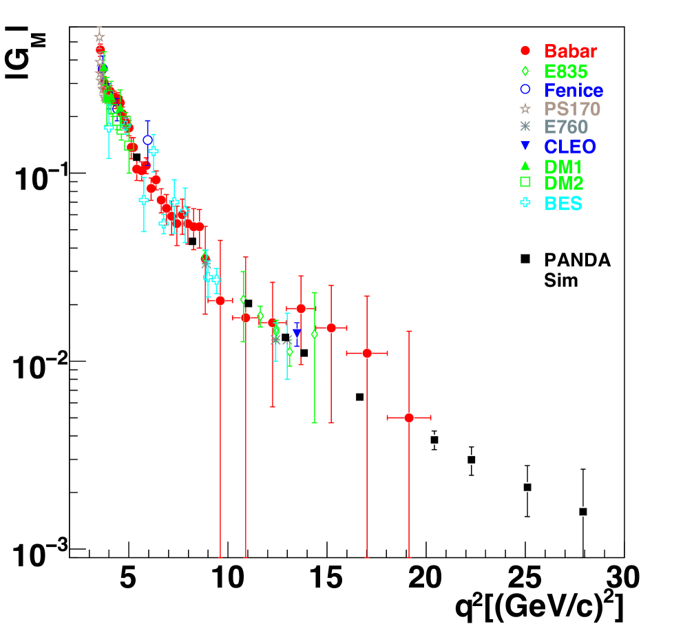
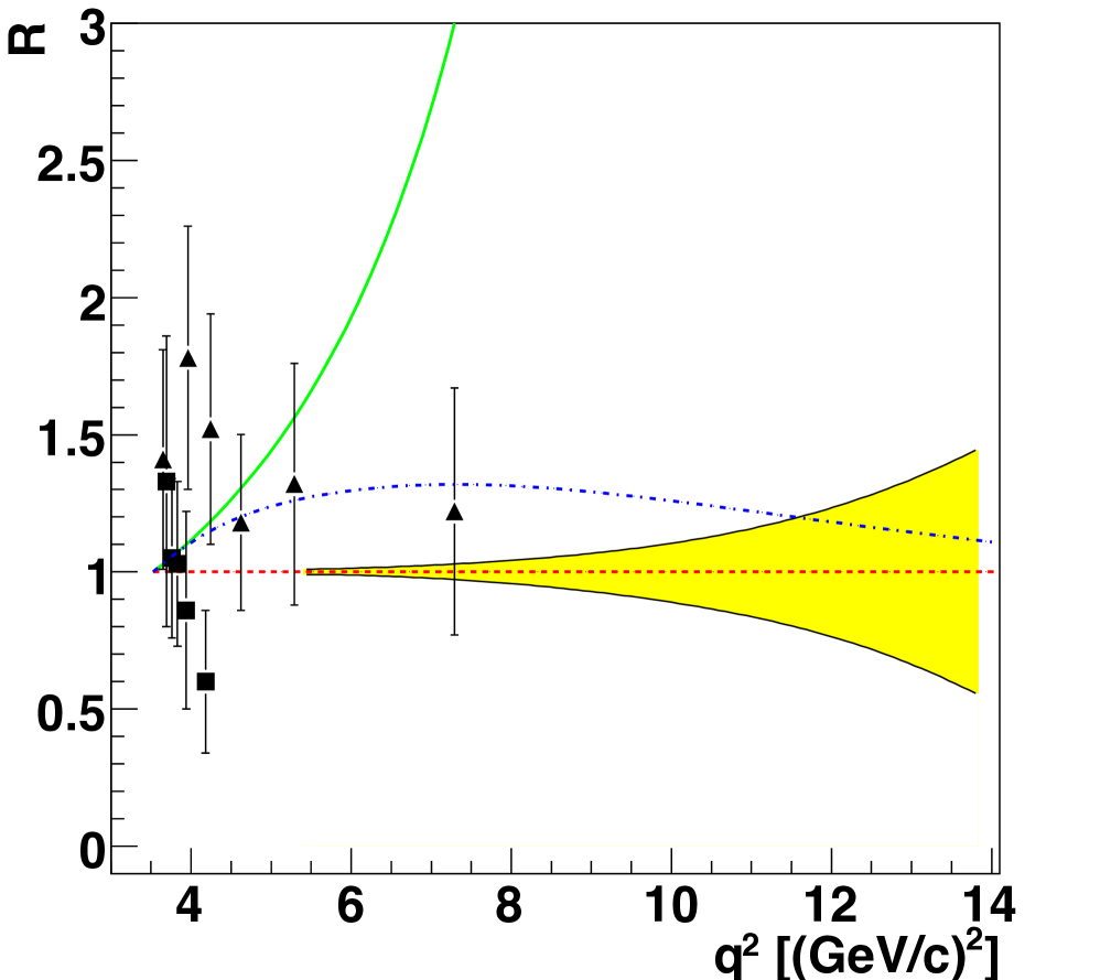
In Figs. (21) and (21) the results of the above-mentioned feasibility studies are summarized. Fig. (21) shows the expected accuracy for the effective FF in comparison to already existing data. In the case of PANDA, an integrated luminosity of fb-1 collected at different values (i.e. scan points) was assumed; only the statistical error is shown. According to Fig. (21) we can expect a remarkable improvement with respect to the so-far most precise measurement from BaBar. Fig. (21) shows the accuracy (yellow error band), which is expected at PANDA for the ratio (for this simulation it was assumed ). In the range between (GeV/c)2 and (GeV/c)2 the statistical error of the extracted ratio will be on the level of a few percent only. Above (GeV/c)2 the extraction of the ratio is not feasible anymore due to the kinematic suppression of (cf. Eq. (4)). It is obvious from Fig. (21) that a precision measurement of the ratio at PANDA will be very sensitive to distinguish between different hadronic models. Three of those theoretical predictions are shown in Fig. (21). The work corresponding to the red dashed line, cf. Ref. [65] (Brodsky, and Farrar), is predicting ; the green solid line and the blue dot-dashed line are taken from Refs. [66] (Iachello, Jackson, and Lande) and [67] (Lomon), respectively. Those models will be further discussed in Sect. 3.
The PANDA collaboration has also suggested to measure the TL em FF of the proton in the unphysical region () by using the reaction , cf. Refs. [63]. Furthermore, it has been demonstrated that TL measurements provide valuable information to search for two-photon effects, cf. Ref. [64].
As mentioned above and as worked out in Ref. [68], future directions in experiment
should concentrate on an experimental
programme, which is aiming for a measurement of the relative phase between the electric
and the magnetic FF’s. In order to achieve this goal, a polarized target, or – as an alternative – a polarized
antiproton beam is required444In principle this phase can be also measured in the case of
annihilation using an unpolarized beam, but measuring the polarization
of the outgoing proton. No experiment at an collider has however taken this into account.
A polarimeter (e.g. made of carbon) would be required for this task.. At PANDA, feasibility studies for a polarized hydrogen
gas target are underway [71], while within the PAX collaboration [72] at FAIR
solutions for antiproton polarization are being investigated. Spin filtering experiments
are carried out in this context – so far with protons – indicating that this method
seems to be a promising
method (cf. Ref. [73]) for nucleon polarization. Hopefully this approach can be tested
soon also with antiprotons.
Double polarization experiments using both a polarized target as well as a polarized antiproton beam
will be giving further insights concerning the relative phases between the magnetic and the
electric FF’s, cf. Refs. [69, 70] for further details.
In Sect. 3.2 we will be discussing in detail the opportunities which are given by
the polarization degrees of freedom.
The various plannings and future
directions outlined in this Subsect. make us
confident, that the experimental progress expected for the coming years will bring us new and enlightening
insights towards a quantum field theoretical understanding of the physics of
TL nucleon FFs. We stress once more that future polarization experiments are a must.
3 Theoretical background
The theoretical investigation of the nucleon em FF’s in the TL region cannot be kept separate from the corresponding one in the SL region, given the complementary nature of the information on the nucleon internal structure, that can be accessed through the electron-nucleon elastic scattering and the annihilation processes or , all related via the crossing symmetry. Therefore, it appears useful to briefly illustrate some generalities on the nucleon FF’s in the SL region. We remind that in a SL scattering process a virtual photon with a four-momentum hits a nucleon with four-momentum . The following relation holds for SL processes: .
3.1 Nucleon Form Factors in the SL region
As it is well-known, in the SL region the nucleon em FF’s can be investigated through the elastic reaction
pictorially illustrated by the diagram in Fig. (22), where the one-photon-exchange approximation is shown. Within such an approximation, a virtual photon () is exchanged between the incoming electron and the nucleon target, in a -channel process. It is compelling to immediately mention the relevant role, which the polarization degrees of freedom played during the last decade in the experimental studies of the proton FF’s (see Ref. [2] for recent reviews). In particular, by applying a novel experimental technique, the so-called polarization-transfer technique, it has been discovered a totally unexpected feature of the electric FF of the proton: a fall-off faster than the dipole one, for (see below).

For , the nucleon em current operator is a Hermitian operator, that behaves like a four-vector under Lorentz transformations, and, moreover, fulfills the constraints imposed by parity, time-reversal and current conservation. These general properties straightforwardly lead to the following covariant expression for the matrix elements in the SL region (see e.g. [74],[75] and [76]).
| (6) |
where i) and are the initial and final nucleon spinors (normalized as ), and ii) and are the Dirac and Pauli form factors, respectively. They are scalar functions that depend upon one scalar quantity, , namely the only, non trivial kinematical scalar constructed through and . The second line in Eq. (6) has been obtained by applying the Gordon decomposition. It is worth noting that, in the first line of Eq. (6), the Dirac structure allows a physically grounded classification of the two terms. As a matter of fact, one has a helicity conserving contribution, that fulfills and a helicity non-conserving term,that fulfills , (let us remind that is the helicity projector for an ultra-relativistic case).
The Dirac and the Pauli form factors take into account the non-elementary nature of the nucleon, and they are normalized according to the proton and neutron charges for and to the anomalous magnetic moments for , viz
| (9) |
Notably, in the SL region, the Dirac and Pauli FF’s are real functions. This feature can be deduced by using the Hermiticity of both and the Dirac structure ( and ). One could infer the Hermiticity of , by observing that the first-order approximation of the T-matrix is a Hermitian operator in the SL region, since in the -channel no real particles can be present in the intermediate states. In particular, the unitarity condition for the first-order T-matrix, , reads
| (10) |
As mentioned above, the vanishing value of the rhs is due to the unphysical nature of the intermediate states, . Then, the Hermiticity of follows from the Hermiticity of . It is important to anticipate that, in the TL region, the unitarity constraint has to be implemented by taking into account the opening of real-particle production channels, since a -channel reaction occurs. Therefore, the TL nucleon FF’s are expected to be complex functions.
Instead of using Dirac and Pauli FF’s, it is possible to introduce proper combinations of them [77, 75] as follows
| (11) |
where , . In Eq. (11), and are the so-called Sachs electric and magnetic form factors, respectively. The physical motivation of considering these combinations is given by the analysis of the current operator performed in the Breit frame, where and . In this frame, the nucleon FF’s can be expressed in terms of three-dimensional Fourier transforms of functions to be interpreted as electric and magnetic densities, like in the non relativistic framework, viz
| (12) |
where . If , the non-relativistic limit is immediately recovered. Therefore, one could naively argue that the SL nucleon FF’s yield information on intrinsic properties of the nucleon. Unfortunately, such a correlation should be carefully reconsidered, taking properly into account the boosts to be applied to the states of a composite system, like the nucleon (see, e.g., [78, 79]). Notice that, in the Breit frame, both initial and final states have to be boosted when the matrix elements of the current are calculated.
Recently, a new physical interpretation of the nucleon FF’s has emerged (see, e.g. [80]). It is based on the field theoretical description of the constituents, inside the nucleon, given in terms of the so-called Generalized Parton Distributions (GPD’s) (see, e.g., [81] for an extended review of the topic). Such a formalism, developed within the Deep Inelastic Virtual Compton framework, leads to a description that fully satisfies the general principles, allowing to correctly treat the relativistic-boost effects, as well. It should be pointed out that GPD’s depend upon three scalar invariants: , and , with i) the average four momentum of the active constituent, before and after interacting with an external probe, and ii) a light-like four-vector. Furthermore, it turns out that, in the Deep Inelastic Scattering (DIS) limit where the variable plays an analogous role of , one can reobtain the nucleon FF’s from the unpolarized quark GPD’s, putting and integrating on . To complete the analysis, two-dimensional Fourier transforms of the relevant GPD’s in the Drell-Yan frame (a particular Breit frame where the ) are introduced. In this frame, the variable has only transverse components, i.e. , (notice that in the Drell-Yan frame ) and it is conjugated to the impact parameter . In conclusion, the main outcome is given by the determination of well-defined density distributions of the constituents in the transverse plane . For instance, the Dirac FF yields
| (13) |
where is one of the unpolarized GPD’s. Summarizing, can provide information on the density distributions in a transverse plane, once the effect of the boosts on the initial and final states of a composite system are correctly taken into account. This can be implemented by using the light-cone description of both the operator current and the nucleon states (see, e.g., [81]).
The last issue to be mentioned, that will be relevant also in the TL region when a model builder has to constrain his own approach, is the asymptotic behavior of the nucleon FF’s, as dictated by QCD. By considering both dimensional scaling laws and helicity conservation, perturbative QCD (pQCD) yields the following asymptotic behavior for the nucleon FF’s (see, e.g., [65, 82])
| (14) |
where is the anomalous dimension (, depending upon the active number of flavors ). It should be pointed that the asymptotic behavior of the FF’s is dictated by the perturbative gluon exchange, that provides the mechanism for sharing the momentum transfer among the constituents. In order to accomplish this, at least two massless gluons must be exchanged, and each gluon propagator contributes with a factor . As to , the spin-flip effect adds an extra factor .
To complete this snapshot of the SL region, it is impossible to avoid few words on the experimental technique that has given a new, strong impetus to the investigation of the proton FF’s in this region. In particular, a technique based on the measurement of the polarization of the final state proton has experimentally proven that the proton charge FF strikingly decreases faster than the dipole FF [2]. It is also worth noting that in the TL region, since the nucleon FF’s become complex functions, a pair, produced in the final state, naturally acquires polarization degrees of freedom, even in absence of polarized leptons in the initial state (see Subsect. 3.2 and [68]).
In the SL region, when a polarized electron hits an unpolarized nucleon target, some polarization is transferred to the recoiling nucleon. Such a polarization can be measured with a suitable secondary analyzing reaction. The polarization-transfer method (see [2] for more details) is based on the measurement of the transverse and longitudinal components of the recoil proton polarization, in the elastic reaction
| (15) |
where the incident electron has a longitudinal polarization along the direction of the momentum transfer, (indeed one could consider reactions with more complicate polarization set-up [83])). To understand why the final state proton gets a polarization, one should first recall that the polarization of a fermion (with four-momentum and spin ) with respect to a given direction, , is obtained from the following expectation value:
| (18) | |||
| (19) |
where . In order to determine the polarization of the final proton, Eq. (19) has to be properly weighted by using the polarization density of the final state, i.e. by exploiting the transition probability to scatter the final proton along a given direction. To this end, one has to use the density matrix of the final nucleon, formally written as , where the matrix is the T-matrix relevant for the process under scrutiny555In a non relativistic framework, one parametrizes , with and complex functions, and . (see, e.g., [83] for a discussion in one-photon approximation within a relativistic framework). It is worth noting that the density matrix of the final nucleon can lead to a polarization in different cases: i) in case the initial nucleon has a polarization, ii) if the incoming beam has a polarization, or iii) a complex-valued FF’s of the nucleon are present in the current (see [84] for the non relativistic case, and [68] for the relativistic one). In conclusion, the above mentioned weighting of Eq. (19) amounts to obtain the polarization of the final proton by evaluating the polarized differential cross section, where an average on the spin of the initial proton is performed (this means an initial density matrix purely scalar), and the polarization of the incoming beam is taken into account. Then, the experimental polarization, , of the recoiling proton is given by (see, e.g. [85] and [84])
| (20) |
where is the unpolarized cross section (representing the normalization of the polarization density matrix in the final state), a proper factor, the leptonic tensor with both symmetric and antisymmetric terms (since the electron beam is polarized in (15)), and the proton tensor is given by
It turns out that the proton in the final state of the reaction (15) gains a polarization in the scattering plane, , taking . The measured components of the polarization vector allows one to extract the ratio of the proton FF’s as follows
| (21) |
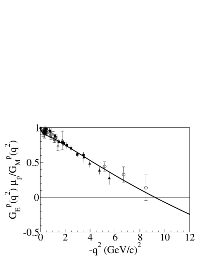
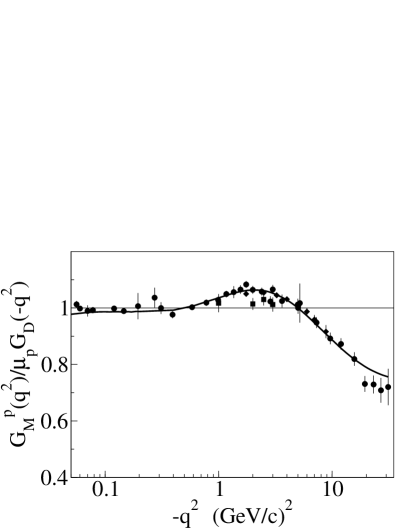
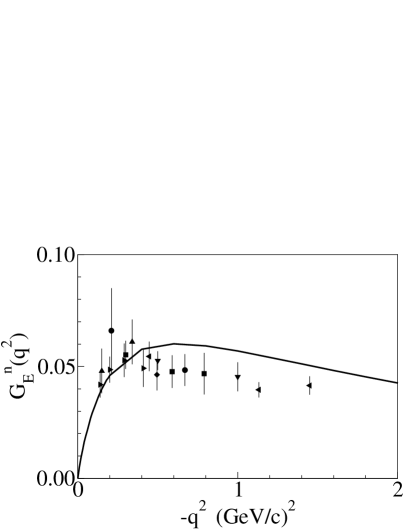
Concluding this Subsection, for the sake of illustration, an overview of the status of the analysis of the nucleon FF’s in the SL region is presented in Fig. (23). It is also shown a recent theoretical calculation [7], based on a relativistic constituent quark (CQ) approach, that has been extended to the TL region, as well (see Subsect.3.9). The interested reader can be referred to, e.g., Ref. [2] for a comprehensive and updated discussion of the experimental measurements.
3.2 Nucleon form factors in the TL region

The reaction where a pair annihilates into charged leptons, viz
| (22) |
and the time-reversed process, viz
| (23) |
represent a direct source of information on the nucleon FF’s in the TL region. For the sake of concreteness in what follows it will be considered the annihilation. In Fig. (24), the one-photon approximation of the reaction (23) is depicted.
In the hadronic annihilation process, a virtual photon with invariant square mass can materialize into a quark-antiquark pair, since it can become active the hadronic part of the virtual-photon state, shortly given by
| (24) |
An honored, and still very alive, approximation of the photon vertex is the vector dominance model (VMD) (see, e.g., [3] for a recent review), that describes the hadronic part of the photon wave-function through a direct coupling between the virtual photon and a vector meson (with the proper mass, spin and parity). Such a model certainly allows one to construct a very effective scheme of approximation, that has to be completed by a description of the hadronic decay of the vector meson, if one is interested in the hadronic FF’s (i.e. ). In view of the quark content of the hadronic term, one should also consider a direct coupling to a pair, and therefore more complicate production channels (as it will discussed in what follows). With these first physical insights in mind, we can start to deal with the analysis of the matrix elements of the nucleon current for describing reaction (23).
The investigation of the process (23) (as well as (22)) takes advantage of the crossing symmetry, and therefore one can exploit the previous analysis of the elastic scattering in the SL region. In particular, the matrix elements of the nucleon current operator involved in the reactions (23) are written as follows
| (25) |
where , and , in the center of mass. In the TL region, the current operator is involved in the transition from the vacuum to a state with a nucleon-antinucleon pair, that becomes real beyond the proper threshold, given by . This means that production channels are now opened, and therefore the current operator is not more a Hermitian one. This can be verified from the unitarity condition, Eq. (10), applied to this case, namely to an -channel process. As a consequence, as it can be also recognized from a perturbative analysis of the FF’s themselves, the nucleon FF’s become complex functions, with a characteristic multi-cut structure due to the free propagation of the relevant hadronic pair, beyond the proper production threshold. Indeed, if we expand the analysis to include the whole hadronic production, one can recognize that different channels can be opened, with different energy thresholds. In the interval , there is no purely hadron production at all, while for increasing values of , up to , one meets channels that contributes to the production of a virtual pair. One has in order : i) the isovector two-pion channel, that starts at , where is the pion mass, ii) the isoscalar three-pion channel, that begins at , iii) the meson production, beyond , etc. The physical threshold for the is and the region is called the unphysical region, when we are dealing with the reaction (23): it contains many interesting information, particularly near the threshold (see Subsect. 3.3). It should be pointed out that the opening of more production channels beyond the threshold generates new overlapping cuts in the FF’s. As we will see below (Subsect. 3.4), one of the main issue in the general treatment of the TL FF’s is precisely the evaluation of the discontinuity of the FF’s across the cuts, namely the imaginary part of the FF’s.

By adopting the one-photon approximation and performing the suitable traces, one gets (see also Eq. (4)) the following differential cross section for the -pair production, in the CM frame, [86] (for the cross section of the reaction see Ref. [87], paying attention to the flux factor different from , in this case)
| (26) |
where , is the angle between the direction of the incoming electron, taken as -axis, and the produced nucleon (see Fig. (25)), the absolute value of the velocity of both and (with ), (notice the difference with the definition in the SL region, below Eq. (11)) and is a constant defined as follows
| (30) |
with
(notice that the expression of the variable contains a factor at variance of what one can find in Ref. [9] where a mistyping is present [88]). In the case of the -pair, is the s-wave Sommerfeld-Gamow factor that takes into account the QED leading-order correction to the wave-function of the charged pair, and results to be proportional to , where is the relative wave-function in the continuum. This factor specifically affects the cross section near the threshold, where the relative 3-momentum of the charged hadronic pair is small (see, e.g., [89, 90]) and therefore . In particular, it makes the cross section different from zero at threshold, since the factor in the denominator of balances a factor that comes from the phase-space calculation. As a final remark, it is worth noting that the standard non relativistic expression of the variable is
where is the relative velocity, the relative momentum and the reduced mass (). It can be heuristically generalized to the relativistic framework [9] as follows
obtaining the expression of the variable in Eq. (30) (notice that in the above equations).
In Eq. (26), as in the SL case, one has introduced the Sachs FF’s, given by
| (31) |
Notably, at the threshold, i.e. , electric and magnetic Sachs FF’s become equal by construction. This issue has been experimentally investigated for the proton case, by two different collaborations. As discussed in Subsect. 2.2, the ratio has been extracted from the angular distributions (cf. Eq. (26)) measured in a wide range of momentum transfer, (GeV/c), by the BaBar collaboration [9]. For up to (GeV/c), the ratio results to be significantly greater than unity, in disagreement with previous data, obtained by the PS170 collaboration [10], that are compatible with the expected threshold value .
The total cross section in one-photon approximation is obtained from Eq. (26) by integrating over the solid angle . For the sake of legibility, here we rewrite Eq. (1), but with some obvious changes, viz
| (32) |
Such an expression suggests to define an effective nucleon form factor in the TL region by dividing the actual total cross section shown in Eq. (3.2), by the point-like one, obtained from Eq. (3.2) putting . Then, one can write
| (33) |
where
| (34) |
The total cross section becomes
| (35) |
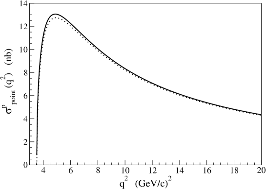
The point-like cross sections for proton and neutron reduce at threshold, i.e. , to
| (36) |
where for the neutron for . In Fig. (26), for illustrating the effect of the Sommerfeld-Gamow factor and the behavior close to the threshold, for both proton and neutron, is shown in the range of the present-day experiments. One should notice i) the very steep increasing between the thresholds, and respectively, and the maxima, around , and ii) the effect of the Sommerfeld-Gamow factor that makes non vanishing the point-like cross section of the proton. at the threshold.
Coming back to the definition of the effective FF, that in one-photon approximation is a combination of electric and magnetic Sachs FF’s, it appears quite natural to compare Eq. (33) with the corresponding quantity defined through the experimental cross section , namely Eq. (2). It should be pointed out that in both numerator and denominator in the middle of Eq. (2) there are quantities experimentally measured, and therefore one has an operative definition for , a part the model dependence due to the Sommerfeld-Gamow factor. Moreover, in analogy with the microscopic interpretation of the SL FF’s as Fourier transform of electric and magnetic spatial distributions (cf Eq. (12) with the caveat of Eq. (13)), one could develop a simple physical picture of the TL effective FF. Indeed, one could consider that it is microscopically related, through a Fourier transform in time, to the transition amplitude from a virtual-photon state (cf Eq. (24)) to a hadronic state. With this in mind, it becomes clear that in the TL region one can explore the time/energy structure of the hadronic Fock components of the photon state. At this point, a final short comment about seems appropriate. One should notice that, unfortunately, in the literature one can find a shortcoming in the presentation of what the experiments provide. As a matter of fact, sometimes it is claimed that one measures the nucleon magnetic form factor assuming , but this is not the case, unless (i.e. at the threshold). However, it should be clarified that the proton database in the TL region, is entirely constructed by introducing the effective proton form factors as defined in Eq. (2). For the neutron case, the Frascati data points [13] are shown i) by using Eq. (2) or ii) by assuming , that amounts to define for the neutron
| (37) |
In any case, in the experimental papers the procedure adopted for extracting the data is always properly indicated.
In the TL region, since the nucleon FF’s are complex functions, one has extra degrees of polarization for the produced pair, even without a polarization of the incoming beams. This was already explained above, in the brief introduction to the polarization-transfer method in the SL region. For instance, one finds that a produced proton [86, 91, 68] gains a polarization perpendicular to the scattering plane (recall that the chosen -axis is directed along the incoming electron beam) and, in one-photon approximation, it is given by
| (38) |
where is the phase of the complex-valued electric (magnetic) Sachs FF and is defined as:
| (39) |
The other two components of the polarization, and , lie on the scattering plane and are different from zero only if the electron beam has a non vanishing longitudinal polarization, , viz
| (40) |
As one can see from Eqs. (38), (39) and (26), information on absolute values and phases can be extracted by measuring both the angular distributions and the normal (to the scattering plane) polarization. Indeed, one could consider also different cases, e.g. a polarized antiproton beam in the reaction (22) [72], in order to extract double-spin polarization observables, that allows to access (see Refs. [69] and [70] for details).
The previous expressions of both cross section and polarizations have been obtained by considering only the one-photon-exchange approximation. The formalism for including the two-photon-exchange effects can be found, e.g. in Ref. [92] (for a recent review of the effects of the two-photon exchange in the SL region see Ref. [93]), while Refs. [94, 95] give a first quantitative investigation of the effect, showing a reassuring smallness (few percents) of the corrections.
3.3 The production threshold
The study of the reaction (23) near the threshold provides many relevant insights in the reaction mechanism that governs the transition from the unphysical to the physical regions.
For the proton case, the PS170 collaboration [10] observed for the first time a steep slope of the effective FF when slightly increases from the threshold value, and more recently the BaBar collaboration [9] has accurately measured and confirmed the near-threshold peak. As to the neutron, the FENICE collaboration [13] (see also [12] for the proton measurements) made the first and (till now) only measurement close to the threshold, showing also in this case, but with large error bars, an increasing value for .
The sizable and sharp rising of the cross section close to the production, given the experimental efforts devoted to its investigation, has driven a lot of theoretical studies, pointing to elucidate the origin of such a surprising result. It is useful to remind that for the pion, one meets a more soft behavior, since a huge peak related to the -meson production, around MeV, appears far beyond the production threshold of a pair, . Even if the proposed mechanisms for explaining the proton case are different, all the approaches have the common aim to clarify and constrain the interaction. In particular, the steep slope has been explained i) by the final-state interaction acting near the threshold (see, e.g. [97] and references quoted therein), ii) by the tail of a bound state (see, e.g. [98] for a recent investigation of this issue by using the Paris potential and reference quoted therein) or iii) by a narrow meson resonance [13], just below the threshold. For instance, in Ref. [99] a complex scattering length in a state is obtained from the Jülich potential [100], allowing to achieve a good description of the data. In Ref. [97], the field of investigation is enlarged to cover not only the proton case but also and other systems, by exploiting a phenomenological approach beyond the scattering-length approximation, pointing to a resonant behavior near the threshold. The bound state appears a very intriguing possibility, but such an explanation as mentioned above, is in competition with less exotic effects. However, if this is the case, one could address the issue via reactions like or even as investigated in [101], by taking into account the off-mass-shellness of the nucleons inside the target nucleus.
The neutron threshold deserves some attention, in view of the existence of only one data set [13]. Those data posed a question about the applicability of a naive pQCD analysis to the production involved in the proton and neutron FF’s. By using the FENICE data for both proton and neutron, one has , while a naive perturbative description of the annihilation [102] leads to , namely almost a factor of difference. Fortunately the new data by the BaBar collaboration [9] suggest a path that reconciles experiment and naive expectation, since by considering the BaBar proton data near threshold, the difference between the experimental ratio and the naive pQCD prediction shrinks the difference to a factor of , but with a large error band, due to the uncertainties of the FENICE neutron data.
3.4 Dispersion Relations: an overview
A truly microscopic calculations of the nucleon FF’s have necessarily a prerequisite: i) a knowledge of the substructure of the nucleon and the interactions between the constituents, and ii) a non-perturbative framework where elaborating the calculations. Such an observation makes clear how much challenging be the task. Historically, coming back to the fifties, the study of the nucleon FF’s had great benefits from the extension of the investigation to the whole complex plane of the relevant variables. In this way, as briefly illustrated below, the non-perturbative regime of the strong interactions, based at that time on nucleonic and mesonic degrees of freedom, could be taken into account, by exploiting both i) information gathered within a perturbative (diagrammatic) analysis of the needed amplitudes and ii) more fundamental properties, like causality, embedded and tightly related to the analytical behavior of the observables. As it is well-known, such an analytic method has its origin in the Kramers-Krönig relation in optics [103].
Local properties of the field theories, as dictated by the microscopic causality, can be immediately translated into the analytic behavior of the scattering amplitudes (see, e.g. [76]), and in turn into the analytic behavior of the general Green functions of the interacting fields, if one adopts the Lehmann-Symanzik-Zimmermann (LSZ) reduction formula [104] for the S-matrix elements.
The causality constraint imposes a finite value for the speed of any signal. This constraint can be rephrased into the request that space-time regions, separated by space-like distances, cannot communicate each other and therefore one has to require proper operatorial relations between fields, viz
| (41) |
where and are the local bosonic and fermionic fields of a given theory, respectively. In turn, the commutation properties establish well-defined analytic behavior of the Fourier transform of combinations of the field themselves, analogously to the basic investigation performed in classical optics by Kramers and Krönig, who analyzed the propagation of a wave front and found the constraints induced by causality on the diffractive index (i.e. the em response of the composite system). A causal behavior means that the response of the system will be vanishing for , where is the instant when the system starts to be perturbed. If one takes into account such a constraint, one can rigorously deduce that the Fourier transform of the system response must be analytic in the upper-half plane (see [76] for details). Then, an integral relation between the real and the imaginary part of such a Fourier transform follows. For instance, if one has a complex function , analytic in the upper-half plane, one can write the following Cauchy integral
| (42) |
with a contour, , composed by the real axis and a semi-circle at infinity, in the upper half-plane. If properly behaves for , namely the contribution from the arc at infinity is vanishing, one gets a simple expression
| (43) |
otherwise one has to add the contribution of the semi-circle. Moreover, recalling the formal expression
where indicates the Cauchy principal value, the following relations, called dispersion relations (DR’s)666These relations are also known as Hilbert transformations between and ., can be straightforwardly deduced
| (44) | |||
| (45) |
Therefore, the knowledge of the whole function can be obtained from the knowledge of only one contribution: the real part or the imaginary one. The name dispersion relations can be traced back to the work of Kramers and Krönig [103], where the diffractive index was investigated, and relations between the real part (governing the dispersive behavior of the light) and the imaginary one (controlling its absorption) were established, by using the causality principle, as mentioned above.
If the assumed quick fall-off of does not hold, and therefore the integrals in Eqs. (44) and (45) are not well-defined, then one can write down new DR’s, by introducing a proper subtraction term. For instance, for , one can speed-up the fall-off by subtracting and repeating the same steps that lead to Eqs. (44) and (45), but for
obtaining, e.g., for the real part
| (46) |
since . Such a subtraction procedure can be applied with the obvious changes, e.g. subtracting from , as many times as it needs in order to make vanishing the contribution at infinity, in the integrals.
In view of the application to the nucleon FF’s, it is interesting to briefly discuss the case when has a cut for , and it is real for . The Schwarz reflection principle, , applied along the open interval , allows one to analytically continue in the lower half-plane. Then a different path can be considered for writing down the Cauchy relation (42). In particular, the integration path runs along the lower rim from infinity to and along the upper one in the reversed direction, and it has to be completed by a circle at infinity (to be integrated in the counter-clockwise direction). Then, assuming for simplicity that the contribution to the Cauchy integral for is vanishing (a subtraction procedure can be always implemented), one gets
| (47) |
In conclusion, the function is determined for any by the discontinuity across the cut. The relevance of this relation is given by the possibility to link the imaginary part of the nucleon FF’s in the TL region to physical amplitudes, as discussed in the following Subsection. With simple steps, one can also write
| (48) |
Such an equation is a generalization of Eq. (44), where the analyticity of was assumed only in the upper half-plane. In the case of a slow decreasing of for , one can repeat the subtraction procedure as in the previous Eq. (46), obtaining the following one-time subtracted expression
| (49) |
In closing this Subsection, it is important for what follows to mention one of the theorems that can be deduced from the Phragmén-Lindelöf principle that allows to extend the maximum-modulus principle to unbounded domains [105]. The theorem, relevant for putting in relation the asymptotic value of the FF’s in the TL region and in the SL one, states:
If an analytic function , with , is such that i) as along a straight line starting from the origin and as along another straight line, again starting from the origin, ii) it is regular 777A regular function is analytic and single-valued in a given region.and bounded in one of the two sectors between these two straight lines. Then and uniformly in that sector as . It is important to note the request that the analytic function must be bounded in one of the two sectors.
Summarizing the analysis in the complex plane, one should mention four items: i) causality determines the analytic behavior of an amplitude involved in a given physical process, ii) the Schwarz reflection principle allows to analytically continue a function from one side of the plane to the other side, if along a part of the real axis it does not contain singularities, iii) in presence of a cut, the function can be expressed in terms of the discontinuity across the cut, iv) a theorem from the Phragmén-Lindelöf principle leads to relate the asymptotic behavior of the function for . One of the first discussions of the application of the Phragmén-Lindelöff theorem (previously used for proving the Pomeranchuk theorem and its generalizations) to the em nucleon FF’s, putting in relation the asymptotic values in the SL and TL regions, can be found in Ref. [69].
3.5 Dispersion Relations and the Nucleon Form Factors
Refs. [4, 106] (see also [76], [84] and [107] for more general discussions) yielded a first description of how the previous general properties, particularly causality, can be exploited for modeling the nucleon FF’s in both the SL and the TL regions. Noteworthy, the same approach can be applied to any hadron.
In the seminal work of Ref. [4], dispersion relations for the SL and TL nucleon FF’s were determined, after analyzing the matrix elements of the em current operator (needed for the first order T-matrix) and using the LSZ reduction formalism [104] for the S-matrix elements (see, e.g., [76]). A direct and fundamental consequence of such an investigation was the possibility of relating the imaginary part of the FF’s to matrix elements relevant for other physical processes, that, in turn, can offer experimental inputs for an overall description of the FF’s themselves. Let us briefly illustrate the issue in the TL case, by considering the following matrix elements of the em current operator
| (50) |
where, due to the LSZ reduction, one has
| (51) |
with the source of the nucleon interacting field, i.e.
| (52) |
It should be recalled that , like , lowers the baryon number by a unity.
An important step for making more transparent the investigation of the analytic behavior of the FF’s, is the substitution of the time-ordered sum by the commutator , that allows one to implement the causality (cf. also Eq. (41)). This can be accomplished by noticing that the matrix element , generated by the rightmost term in the second line of Eq. (51), does not contribute to the matrix element of the current, Eq. (50). As a matter of fact, since
the matrix element must vanish. Therefore, no contribution can be generated by a one-nucleon intermediate state, when a physical, complete basis is used for spanning the matrix element , viz
| (53) |
where means an integration over the four-momentum and a sum over the discrete quantum numbers. It should be pointed out that the intermediate states spanning the matrix element in the lhs of Eq. (53) must have baryon number , since both the em current conserves the baryonic number and annihilates a nucleon in the initial state. Moreover, (the nucleon is the lowest state), and therefore the intermediate states must contain multi-hadron systems with . Finally, since in Eq. (50) , one immediately deduces that does not contribute to (see also [84] for details). As a matter of fact, one gets
| (54) |
Therefore, the matrix element in Eq. (50) can be rewritten as follows
| (55) |
As mentioned above, the presence of the commutator makes it possible to exploit rather directly the causality, since , is vanishing for space-like separations, i.e. (given the commutation rules of the local fields). Then, one has to deal with two theta functions in the four dimensional integral (55): and . A general discussion, that involves a careful analysis of the dependence in , where and , can be found in [84]. Here, following the simplified presentation of Ref. [4], the case is assumed, and the analytical dependence upon only , taken as a complex variable, is considered. Given the function , the analytic structure of the integrand in Eq. (55) is governed by , and this leads to argue that the matrix elements of the current is analytic in the upper half-plane of . Straightforwardly, one can repeat the steps illustrated in the previous Subsection and construct dispersion relations for the nucleon FF’s. Indeed, if one would use the dispersion relations (see Eq. (47) or its subtracted version, Eq. (49)), one has to fully determine where the singularities are located, and in this task the help comes from the analysis in perturbation theory, namely by considering the Feynman diagrams contributing to the FF’s. Such a study (see, e.g., [76]) shows that in the TL region one meets multiple cuts: a first branch point located at , i.e. in correspondence with the threshold of the two-pion production, that contributes to the isovector part of the nucleon FF’s (in a VMD framework [3], one has the production of a virtual meson, that decays in two pions), then another cut starting from the threshold of the three-pion production, that contributes to the isoscalar part of the nucleon FF’s (in a VMD framework, one has the production of a virtual meson, that decays in three pions), etc. (see below). In summary, within a DR approach one obtains (cf. Eqs. (47) and (49)) the following expressions for the nucleon FF’s, valid for any
| (56) |
where the normalizations of the FF’s have been explicitly shown, with
Moreover, the lowest thresholds for each isospin channel have been considered. Three comments are in order: i) the main task should be the evaluation of the imaginary part of the form factors for , ii) one could expect more cuts starting at various thresholds, depending upon the particle productions one has to consider, iii) one should keep in mind that the dispersion integrals have contributions also from values of below the production threshold (), the so-called unphysical region.
Indeed, the analysis of the discontinuity across the real axis, for , of the current-operator matrix elements allows one to determine the imaginary part of the FF’s, establishing the announced link with physical processes, like the hadronic decays of neutral vector mesons, the TL form factors of mesons (e.g. for describing the -continuum) or the physical annihilation into mesons. To show this, still following Ref.[4], one can write
| (57) |
Notice that i) Eq. (54) has been used, and ii) lowers the baryon number by a unity and therefore the intermediate states must have , as also requested by the matrix elements of the em current . If one repeats analogous steps (illustrated in Appendix A) for the matrix elements of , one can single out the imaginary part of the nucleon FF’s by evaluating matrix elements of the skew-hermitian part of , as follows
| (58) |
From Eq. (58), by applying the proper Dirac traces, one can obtain the needed relations for determining (see the next Subsection). The attractive feature of Eq. (58) is the link with physical processes, as already said. In particular, the matrix elements is related to the em production of physical hadronic systems with , while the matrix elements is proportional to the hadronic production of a pair (or the annihilation into hadronic states). It should be pointed out that, since the intermediate states have , given the presence of the four-momentum conserving delta-function, they represent physical states (differently from the SL case where , i.e. unphysical intermediate states), and a spectral decomposition of the nucleon FF’s can be devised. Strictly related to the value of the masses of the intermediate states, there is the question of the energy thresholds of the multi-cut structure that must appear in Eq. (56). One can immediately realize that the em hadron production, , has as the lowest physical threshold (contributing to the isovector FF’s), while the physical threshold of the hadronic production of the pair , is . The region between these two thresholds, as mentioned above, is the unphysical region, that, however, contributes to the dispersion integral, since the path of integration starts at , i.e. where the free propagation of the pions begins. Therefore, one of the issues in the DR method is given by the evaluation of the matrix elements in the unphysical region. This can be overcome through an analytic continuation of the physical processes and by considering the crossing symmetry (see [4] and [108] for a more recent discussion). Below the threshold , there are other possible energy thresholds related to the em productions of three pions, -pair, four pions, , etc. In particular, one has to remind that the intermediate states, , must have vanishing baryonic number and strangeness, and therefore they can contain two or more mesons, with proper quantum numbers, or baryon-antibaryon pairs. Moreover, given the presence of the matrix elements of the current operator , the intermediate states must have the proper isospin quantum numbers dictated by , that contains an isoscalar term and an isovector one. For instance, the first term filters non-strange meson states with , i.e states with an odd number of pions, while the second term can single out non-strange meson states with , i.e states with an even number of pions. Since the G-parity does not affect states made by strange mesons, the lightest state with a kaon and an antikaon can contribute to both isospin channels.
3.6 TL Nucleon form factors and the dispersion relation approach
The DR approach has been widely adopted for describing the SL nucleon FF’s (see, e.g., [109] and references quoted therein). Particular care was devoted to modeling the spectral representation of the imaginary part of the FF’s (cf. the sum in Eq. (58)). One of the main ingredients for achieving such a description was represented by the phenomenological input supplied by the VMD (see, e.g., [3]), since one could use a physically meaningful scheme and exploit experimental quantities for describing . Moreover, the extension to the TL FF’s was straightforward, since the DR’s hold for any value of . In particular, the DR approach adopted in Ref. [109] for a very accurate description of the SL FF’s (as known at the date), was extended in Ref. [110] to the TL region, without changing the number of the free parameters. For brevity we call this approach the Mainz model. In the spectral decomposition of , it was considered: i) the same numbers of VM poles as in [109], ii) the continuum, already used in the SL region for constraining the overall description through unitarity, and iii) the asymptotic behavior suggested by pQCD (cf. Eq. (14)), including in this way both hadron and quark degrees of freedom. For the sake of concreteness, let us mention that the spectral decomposition in terms of the VMD model amounts to a finite sum on the intermediate states with masses equal to the relevant vector mesons, viz
| (59) |
where and , and contains all the information about coupling and the transition . The above result follows from the VMD contribution to the whole FF’s, viz
| (60) |
where . Notice that the denominators, that come from the VM propagators, vanish only for , and produce the well-known pole pattern, experimentally seen in the TL region(cf Subsect. 2.2).
In [110], it was assumed an unsubtracted form for DR’s, that allows one to write
| (61) |
where the function , given by
| (62) |
takes into account the pQCD prescription for the asymptotic behavior. In the second line of Eq. (61), describes the two-pion contribution, including both the term from the pole and the continuum. This last term is parametrized through the pion form factor and the P-wave partial wave amplitude, without free parameters (see [109] for details). It is worth recalling that by using Eq. (62) one can recover the standard pQCD behavior for , viz
| (63) |
that, in turn, can be properly continued in the TL region. In Eq (62), is the anomalous dimension, controls the transition to the pQCD behavior and . In the actual calculations, the constants were chosen as follows: , corresponding to a number of flavors , , while the adjusted parameters were: i) the quantity and ii) the residues , corresponding to the contributions from three meson poles for each isospin channel. In particular the masses of the vector mesons were: , , , , and . Results for the TL nucleon FF’s, obtained by applying the Mainz model, are shown in Fig. (27).

The work described in Ref. [110] has been steadily improved by the Mainz-Bonn-Jülich collaboration [111, 108], enriching the previous description both i) by adding the as well as the continuum, and ii) by updating all the experimental inputs with latest experimental results. Moreover, different ways for implementing the asymptotic behavior requested by pQCD (see Refs. [111, 108] for more details) were considered. In particular, in the most recent SL and TL calculations presented in Ref. [108], it was introduced the so-called superconvergent approach for controlling the asymptotic behavior of the TL nucleon FF’s, besides the standard one given by Eq. (63). The superconvergent approach amounts to impose a proper fall-off not only to the real part (cf. Eq. (63)), but also to the imaginary part of Dirac and Pauli FF’s, i.e.
| (64) |
It should be pointed out that these constraints allow to take into account the application of the Phragmén-Lindelöff theorem, as illustrated in Subsect. 3.4. The TL nucleon FF’s, calculated by using such a superconvergent approach are shown in Fig. (28). Notice that i) the SL and TL proton data and ii) the neutron SL FF’s have been included in a 17-parameter fit, and therefore the neutron TL calculation (solid curve in the rightmost panel of Fig. (28)) represents a genuine prediction.
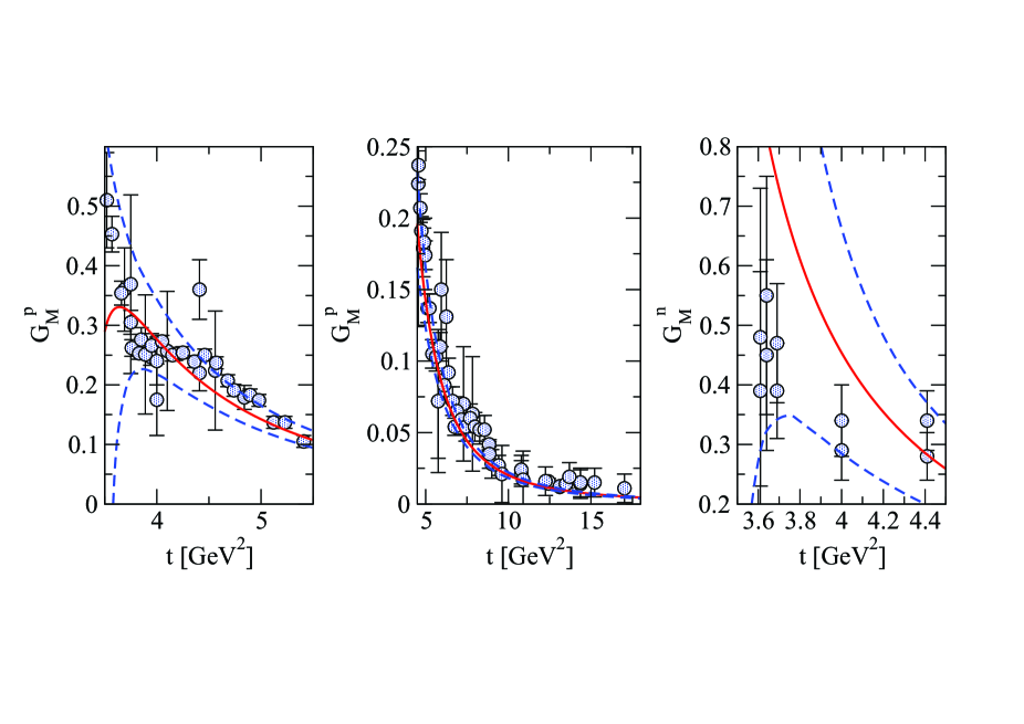
In Ref. [108], it was also presented an explicit pQCD continuum approach, based on a phenomenological Ansatz that fulfills the pQCD behavior (63). In this case the set of free parameters is reduced to 14, but the quality of the fit become worst, as pointed out in the same work.
More recently, the above illustrated approach has been improved by the Tokyo-Chiba group, adding more vector-meson poles and more parameters for modeling the pQCD contribution. In Ref. [112], an unsubtracted DR has been assumed for both Dirac and Pauli form factors, in the SL and TL regions. The spectral decomposition of the is described in an analogous way as in Ref. [108]. It was considered i) a continuum with a helicity decomposition of the amplitude (notice that the tabulated data for the scattering adopted in [112], i.e. the ones by Höheler et al [113], already contain the contribution), and ii) up to 5 meson resonances for each isospin channel, taking into account both mass (up to ) and width in the Breit-Wigner function that describes each vector-meson pole contribution. A particular care was devoted for modeling the asymptotic behavior suggested by pQCD, both considering contributions up to and implementing the superconvergent Ansatz in a slightly different way with respect to Ref. [108] (cf. Eq. (64)), viz
| (65) |
where has to satisfy the asymptotic condition
| (66) |
with and constants. In the actual calculation it was used . With the previous constraints, has the standard pQCD behavior, a part the value of different from the standard anomalous dimension. In the approach of Ref. [112], the number of free parameters has substantially increased, since one has 5 masses and widths for each isospin channel, and correspondingly 10 residues for the vector meson poles of both the Dirac and Pauli FF’s. Therefore the VMD part contains 40 parameters. Finally, one has to add 12 adjusted coefficients for the QCD part, 3 parameters that enter a convergence factor, ensuring the super-convergence condition and another one that shifts slightly the masses of the resonances in the Breit-Wigner width. The 56 parameters are fixed by fitting: i) the most recent SL and TL proton data, even considering the ratio measured by the BaBar collaboration [9] in the TL region (notice a mistyping in [112], where the experimental ratio is indicated with ) and ii) the SL and TL neutron data. The reasonably good description of the nucleon FF’s, achieved by the fitting procedure of Ref. [112], is illustrated in Figs. (30) and (30).
To summarize the investigations presented in this Subsection, one has to stress the richness of information in the TL region, that can be accessed through . Noteworthy, the experimental determination of the relevant phases could strongly motivate future efforts in developing more and more refined theoretical analysis, possibly tightly related to microscopic calculations, in order to establish a close vision on the non-perturbative regime of QCD.
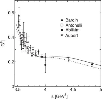
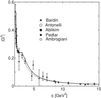
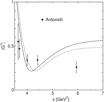
3.7 Phenomenological DR’s and TL extrema
In Ref. [114] the nucleon magnetic FF’s below the threshold, i.e. in the region , has been investigated in an almost model-independent way. The DR’s are adopted for determining an integral equation that relates and where (therefore ), following the modulus representation of the FF discussed in Ref. [115]. In the TL region one writes the following subtracted (recalling that ) dispersion relation
| (67) |
where is the phase of . The range of integration can be split into two parts, and . The integral in the second interval, i.e. the physical region, has been estimated by adopting a suitable function for , with the expected asymptotic behavior, and fitting the available experimental data, assumed to directly give (cf. Eq. (33) for the proper caveat). Then the value of in the unphysical interval, , is obtained by solving the following integral equation, through a very detailed procedure in order to overcome many numerical subtleties,
| (68) |
where indicates the above mentioned integral that depends upon in the physical region. Interesting structures, related to peaks for i) , ii) and iii) near the threshold are automatically generated. Noteworthy, no evidence of a bump at the mass has been found, in spite of the expectation that such a peak should exist if a sizable polarized content in the nucleon were present.
Within the DR spirit, in Refs. [116, 117], the proton ratio has been investigated by considering the following dispersion relation
| (69) |
where . Moreover, the Phragmén-Lindelöff theorem was implemented by imposing a vanishing asymptotic value for , in order to recover a real function when (as in the SL region). As a final step, the imaginary part has been spanned onto the ortho-normal basis given by the Chebyshev polynomials, with independent coefficients for the unphysical and the physical regions. The two set of coefficients are fixed by means of the available experimental data and the theoretical constraints in both the SL and the TL [116, 117], obtaining a description in the unphysical region and also in a wide range of . Unfortunately, the fitting procedure cannot be fully constrained, and this is reflected in the wide band associated to the solution of the integral equation (69). However, interesting results have been obtained, both near the threshold and in the asymptotic region. In particular, a dominance of near threshold has been found, as indicated by a growing ratio up to for . As to the asymptotic region, the moduli of the ratio are quite similar, but the prediction based on the Phragmén-Lindelöff theorem cannot be immediately tested. As a matter of fact, the SL result for is negative for , and in the TL region the extracted value is only the modulus . Therefore the phase of for has to be determined, for a full comparison. Indeed, in order to fulfill the equality between the SL and TL asymptotic values, i.e. (as dictated by the application of the Phragmén-Lindelöff theorem; cf. Subsect. 3.4), one should expect that , since asymptotically is negative. From such an observation, one can deduce the following interesting result. If one applies the argument theorem [105] to a closed path, composed by a circle at infinity and the upper and lower rims of the cut , and reminds also the Schwarz reflection principle, one gets that , where is the number of zeros (poles) inside the closed path. Notice that , given the assumed analyticity inside the closed path and one can choose . Therefore, must be an odd number to fit a negative value for . This seems to be in nice agreement with the SL data suggesting the existence of at least one zero (cf. in Fig. (23)). Further analyses of the issue have been carried out in Ref. [117], where it has been discussed the large uncertainty that affects the modulus of the previous ratio, due to the choice of the data set that one adopts for constraining the high momentum part of . In particular, one gets
Summarizing, all the previous results indicate that the phenomenological studies performed through the DR’s are a source of highly non trivial information in both the extrema of the TL region, given the powerful tool represented by the complex analysis.
3.8 The analytic continuation of the SL Nucleon FF’s
In the DR approach, in its full glory, the main issue is given by the attempt of exploiting physical processes for modeling the imaginary part of the nucleon FF’s, or better the discontinuity of the current matrix elements across the multi-cut region for . As we have seen in the previous Subsections, the knowledge of the imaginary part of the nucleon FF’s allows one to determine the FF’s themselves in the whole range of . A different program is presented in Refs. [118, 119], where it was proposed a fit of the TL data, starting from a well-known model of the SL FF’s, like the one in Ref. [66], devised in the 1970’s for describing, through a VMD approach (see, e.g., Ref. [3]), the available SL nucleon FF’s, but able to predict the fall-off of the SL ratio recently observed (cf. Subsect. 3.1 and [2]). The simple strategy for generating the TL nucleon FF’s, that are complex functions, is based on the analytical continuation of the SL FF’s, that are real functions of , replacing the dependence upon , with and then using the phase as a free parameter in the fitting procedure to obtain the TL nucleon FF’s. VMD plays a fundamental role in the DR approach for reconstructing , since it provides the pole structure, to which one has to add the multi-cuts generated by the free propagation of the hadronic states. Therefore the VMD content of the SL FF’s allows one a first approximation, that can be enriched by using the adjusted parameter . Indeed, only an infinitely accurate knowledge of the SL FF’s (i.e. only in a mathematical realm) could univocally determine the FF’s in their analytical domain, but this is not the case within the realm of the phenomenology.
Refs. [118, 119] have generalized the SL model of Ref. [66], where the external photon couples to both an intrinsic structure, described by a proper form factor and a meson cloud, obtained within the VMD framework. It should be pointed out that the presence of the intrinsic form factor has a clear physical motivation: the size of the constituent quarks (CQ’s) inside the nucleon (see, e.g., Ref. [120] for a discussion of the CQ FF in a relativistic description of the SL FF’s with a realistic nucleon wave-function). In particular, the SL model is given by
| (70) |
where
is the intrinsic CQ FF, , , . The six free parameters, , , , , and are fitted to the SL data.
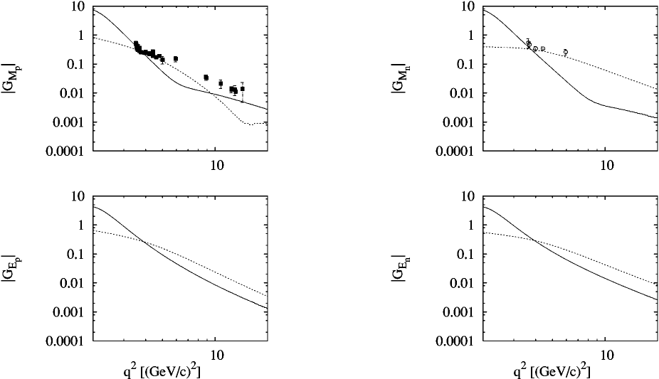
It is worth noting that the asymptotic behavior of the previous parametrization is the same predicted by pQCD, without logarithmic corrections. Moreover, in order to take into account the non negligible width of the meson, the propagator is changed accordingly to
with and being adhoc functions. The value of the fitted phase was found to be in Ref. [118], and in Ref. [119], where the proton data at the largest values were not included. In the upper panel of Fig. (31), the theoretical magnetic FF’s, and , are presented and compared with the experimental data, that correspond to the effective nucleon FF’s (see Eq. (33) and the relative caveat). In the lower panel, the TL electric FF’s are also shown. Unfortunately, as illustrated in the case of , the model does not contain the structure in resonances shown by the TL data for (the adopted VMD stops at the -meson), and therefore the comparison with the experimental data is not satisfactory. As to the neutron, it should be noted the large value reached at the threshold, in agreement with the FENICE measurements [13].
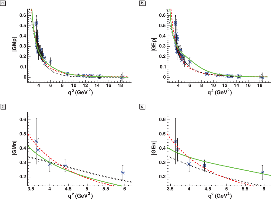
In the same spirit as the previous approach, in Ref. [70] the TL generalizations of both the SL model of Ref. [66] and the SL model of Ref. [67] have been elaborated. In the last case, the 14 parameters present in the SL nucleon FF’s have been updated by fitting the most recent SL and TL nucleon FF’s data-base (see Ref. [70] for the full list). In particular, the generalization to the TL region was performed exploiting the following relations
| (73) |
Together with the above mentioned models, the analytical continuation of a pQCD-inspired model was also proposed, based on counting rules and following the dipole behavior in the SL region. Such a model becomes in the TL region
| (74) |
where is the QCD scale parameter, and are extracted from the fitting procedure to the TL data. The results of the approach of Ref. [70] are presented in Fig. (32). Notice that the SL model of Ref. [67] contains two extra vector mesons with masses: GeV and GeV. Unfortunately, also in this case, the TL data, corresponding to the effective nucleon FF’s, given by Eq. (2), have been compared with both and , separately. In view of this, the comparison proposed in Fig. (32) should be carefully considered at large values of .
3.9 Nucleon FF’s within a Relativistic Constituent Quark Model
A more microscopic description of the nucleon FF’s, in both SL and TL regions, was proposed in Ref. [7], where it was adopted a relativistic Constituent Quark Model (RCQM), already successfully applied to the pion FF in the whole kinematical range [6]. The aim of the approach is to calculate as many quantities as possible in terms of quark degrees of freedom and to perform a direct evaluation of the SL and TL FF’s, without taking care of the DR constraints. At the end, after fixing only four adjusted parameters by using the SL experimental data, one can predict the proton and neutron FF’s in the TL region. In Ref. [7], the following ingredients were chosen: i) the Mandelstam formula [122] for calculating the matrix elements of the current operator in terms of the nucleon Bethe-Salpeter amplitude, ii) a microscopic relativistic Hamiltonian that is able to describe reasonably well the isovector and isoscalar vector meson spectra [123], to be included in the VMD part of the quark-photon vertex, iii) a quark-photon vertex decomposed in a bare term and a VMD term, iv) a Light-front (LF) framework [125], for embedding the previous ingredients and obtaining a relativistic (LF-boost invariant) CQM.
In the RCQM of Ref. [7], the quark-nucleon vertex is described through the Bethe-Salpeter amplitude, with a properly symmetrized Dirac structure, approximated by
| (75) |
where is the isospin spinor, the Dirac propagator of the quark, with the charge conjugation and yields the symmetrized dependence of the vertex function upon the quark momenta, .
In the TL region (for the SL expression see Ref. [7]), the matrix elements of the macroscopic current can be evaluated microscopically by means of the Mandelstam formula [122], i.e.
| (76) |
where in appears , is the quark-photon vertex, the number of colors and the trace runs over isospin and Dirac indexes. Notice that and .
The quark-photon vertex is decomposed as follows
where is the third component of the isospin operator and each term has a purely valence contribution. acting in the SL region only, and a contribution corresponding to the em -pair production (non valence contribution). In turn, the pair-production contribution, i.e. the relevant one in the TL region, can be decomposed in a bare term plus a VMD term (according to the photon-state expansion given in Eq. (24)). For instance, in the SL region, for a CQ with momentum one has
| (77) |
where is the so-called plus component of the quark four-momentum (see Ref. [125] for a detailed review of the LF framework), , and . It has to be pointed out that the constraints and single out a quark or an antiquark, respectively. The constants in the non valence term, (bare term) and (VMD term), are unknown weights determined from a fit to the SL data-base (indeed, in the actual fitting procedure was assumed, see below).
In Eq. (77), yields the VMD contribution to the quark-photon vertex and it has the same structure of the one adopted in the pion case [6], but including the isoscalar vector mesons. For a given isospin channel, is approximated as pictorially illustrated in Fig. (33) (cf. Ref. [6] for more details in the pion case), viz
| (78) |
where is the VM polarization, is the em decay constant of the -th vector meson, the corresponding mass, gives the momentum dependence of the VM vertex function and is the corresponding Dirac structure, while is the running total decay width. It has to point out that in Eq. (78) all the quantities appearing in the numerator have been approximated through the corresponding values calculated at the respective pole (i.e. the residue at ), obtaining, therefore, the correct result when the contribution is maximum. In turn, such an approximation allows one to evaluate , (our Ansatz for the VM vertex function, i.e. the amputated VM Bethe-Salpeter amplitude), by using the eigenvalues and the eigenvectors of the mass operator for vector mesons, proposed in Ref. [123].
The running total decay width in the denominator of Eq. (78), , is vanishing in the SL region, while in the TL region it is assumed to be
| (79) |
where is the total decay width (see, e.g., PDG[124]).
Once the on-mass-shell approximation has been introduced in Eq. (78), is not anymore a four vector, but since only the plus component has to be used in the evaluation of the nucleon FF’s, it is possible to generate matrix elements of the current operator that correctly transform under the LF-boosts (these boosts act on the plus component of a given four-vector without mixing other components, differently from the standard boosts).
Up to 20 isoscalar and isovector VM’s have been considered, since in the case of the pion that number of isoscalar mesons was necessary in order to get fully convergent results for the TL pion FF at the largest experimental values of (). The first four (three) meson masses for the isovector (isoscalar) channel are taken from PDG [124] together with the corresponding total decay widths , while all the other masses come from the solutions of the mass eigenequation [123], and is taken, as in the pion case. Noteworthy, all the em decay constants are calculated from the corresponding eigenfunctions, and they allow the evaluation of the em decay widths , that result in a very nice agreement with the experimental values, when available. Finally, as in the case of the pion, the quark mass is adopted. In conclusion, the VMD part of the photon-quark vertex is fully constrained, a part the relative weights and .

The momentum dependence of the nucleon vertex function in Eq. (75) is differently modeled in the valence region (necessary for evaluating the SL nucleon FF’s) and in the non valence one. In the valence sector, the spectator quarks are on their-own mass-shell, and the 3-momentum dependence, is approximated through a nucleon wave function à la Brodsky-Lepage (pQCD inspired) [125], given by
| (80) |
where is the free mass of the three-quark system, and a normalization constant, fixed through the normalization of the proton charge FF. The power and the parameter are chosen for obtaining an asymptotic decrease of the valence contribution to the SL nucleon FF’s faster than the dipole. The value can be fixed through the evaluation of the anomalous magnetic moments, and , obtaining for those quantities, (Exp.= 2.793) and (Exp.= -1.913).
The non valence vertex, that is fundamental for obtaining a zero in the SL ratio (cf. Fig. (23)) and essential for evaluating the TL FF’s, can depend on the available invariants, e.g. in the SL region one has i) the free mass of the spectator quarks, , and ii) the free mass of the N- system . Then, in the SL region, the non valence vertex is approximated by
| (81) |
where and . The power is a free parameter. In the TL region, the non valence vertex can depend on the mass of the nucleon- system, , and it is given by
| (82) |
where the factor of counts the possible patterns for the gluon emission by the produced pair.
The free parameters determined through a fit to the available SL experimental data, , , and , are four: i) two weights out three present in the pair production term of Eq. (77), i.e. and ; ii) the power in the valence amplitude, Eq. (80); iii) the power in the SL and TL non valence vertexes, see e.g. Eqs. (81) and (82). The minimization yields = 1.7. The overall quality of the SL fit can be appreciated from the comparisons in Fig. (23), and from both the calculated proton charge radius (), and the neutron charge slope at , (exp value; ). Surprisingly, the same quality in the fitting procedure can be achieved by excluding the data [7]. In Fig. (34), the experimental effective FF’s (see Eq. (2)) for both proton and neutron are compared with the RCQM results (evaluated according to Eq. (33)), that are true predictions of the model. It is worth noting that a microscopic calculation could lead to the extraction of valuable information on the dynamical content of a realistic RCQM. For instance, missing strengths at (nicely, the same feature appears in the TL pion FF [6]) and , could point to an enrichment of the present VM data-base, and therefore to a strong request of refining the RCQM approach in the VM sector. This simple example sheds light on the potentially relevant results that one could achieve from the forthcoming accurate measurements in the TL region and more and more improved microscopic calculations.
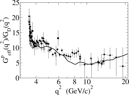
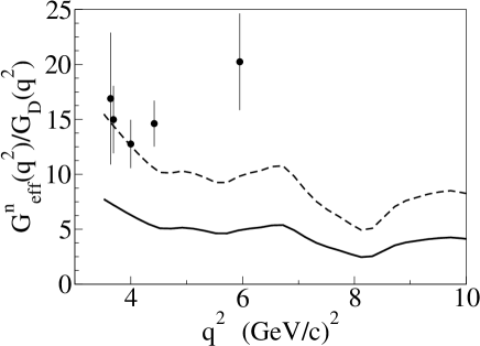
4 Conclusions sand Perspectives
This review has illustrated the advancements achieved so far, both experimentally and theoretically, in the investigation of the timelike electromagnetic form factors of the nucleon. We have also presented the forthcoming experimental facilities, from which in the near future results are to be expected.
The development of the field, started with the pioneering experimental work carried out in Frascati [11, 13] up to the forthcoming exciting experiments with high intensity beams [53, 55] as well as – hopefully polarized – antiproton beams [62, 72] at FAIR, is demonstrating the continuous interest in these challenging studies. However, to measure separately the electric and magnetic nucleon FF’s in the TL region is not an easy task, and the present-day database is still given in terms of an effective TL nucleon FF, that for the electron-positron annihilation process reads (see Eq. (33) and the corresponding remarks):
where the rightmost-hand side shows the relations with the Sachs FF’s in one-photon approximation.
The first success in the experimental investigations was the study of the total cross section for the reaction by exploiting the energy scan technique at electron-positron colliders. In this respect, a major improvement was achieved by introducing the initial state radiation technique, i.e. by using events like (cf. Subsect. 2.1.3). It was possible via ISR to obtain a measurement of the proton form factor with so far unprecedented precision and covering a very wide range. It should be pointed out that the ISR technique is of great appeal also for the planned high-luminosity B-factories, which are mainly devoted to the search of New-Physics signatures in B-decays. The study of the process , lead to single out three energy regions: i) the region around the production threshold, , that yields valuable information on the transition from unphysical to physical regions (cf. Subsects. 3.3 and 3.7); ii) the region where the Vector Meson Dominance and the interplay with the multi-cut analytic structure of the FF’s fully display their phenomenological strength in the studies of the non-perturbative regime of QCD; iii) the asymptotic region where the realm of the perturbative QCD settles and the application of the Phragmén-Lindelöff theorem is representing a fundamental constraint for calculations based on microscopic models. As shown in the theoretical interpretation of the experimental effective FF, (let us recall that such an interpretation is driven by the one-photon approximation and that the two-photon corrections seem to be small in TL region [94, 95, 92]), the electric and magnetic Sachs FF’s are both present in a proper combination (cf. the rightmost side of the above expression). As previously mentioned, experimental efforts already have been carried out [10, 9] and will be pursued in near future with the goal to fully disentangle the electric and the magnetic FF’s. To this end, extending the measurements of the angular distributions (see [9] for recent experimental achievements for the proton case) could provide a tool for determining the ratio . The holy grail in the field of TL nucleon FF’s, however, is the investigation of the phases of the complex-valued FF’s. This is heuristically illustrated in Fig. (35), where the discrimination power of an accurate measurement of the proton polarization perpendicular to the scattering plane, is shown. Notice that does not depend upon the polarization of the incoming electron beam, and once a polarimeter for the measurement of the proton polarization will be included into the experimental apparatus at an electron-positron collider, this measurement of could be performed. The experimental difficulties for achieving such a goal are known and are related to the measurement of the polarization degrees of freedom, but the strong motivations to pursue such a goal were already contained in the seminal work of Ref. [4], where the bridge between the TL FF’s , in particular , and the hadronic amplitudes of hadronic physical processes was established. Therefore, when measurements of will be available, the possibility to extract accurate information on both the em decays of vector mesons and the hadron production (with given quantum numbers) via should allow a carefully study of the hadronic states. From the theoretical side, the starting point of this program has been the analytic behavior of the complex-valued nucleon FF’s, as imposed by the causality, and the consequent dispersion relations (cf. Subsect. 3.4), that link the real and imaginary parts of the nucleon FF’s.
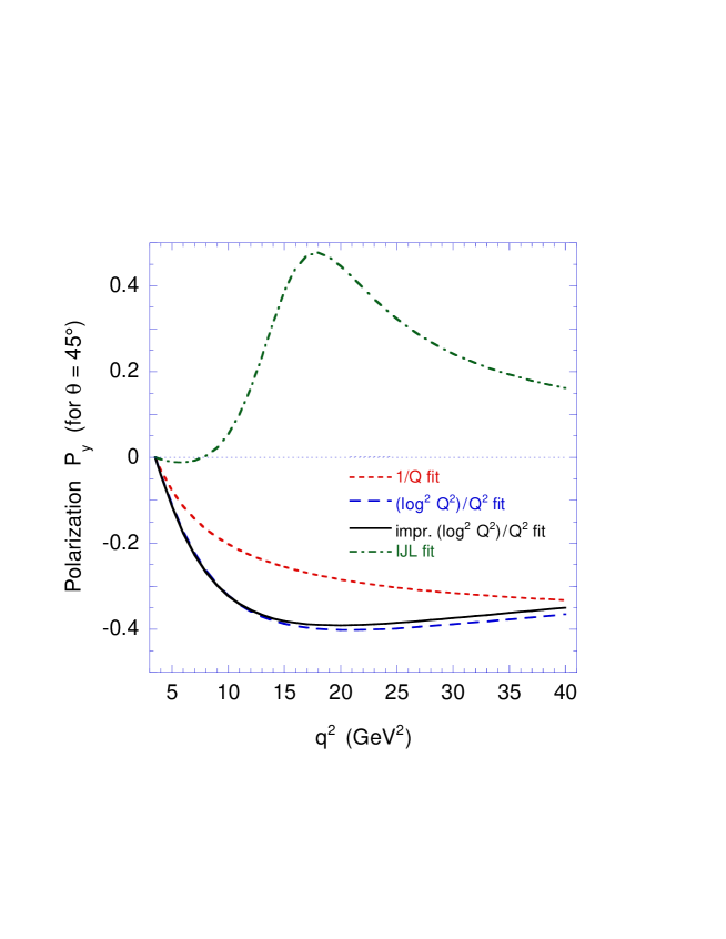
The Lehmann-Symanzik-Zimmermann reduction formula made it possible, to express in terms of the above mentioned hadronic amplitudes, that one can study in other experiments, since they are involved in physical (not virtual) processes. The first phenomenological attempts to model , as shown in Subsects. 3.6, 3.7 and 3.8, were based on exploiting experimental inputs, like masses and widths of the vector mesons, but also i) introducing adjusted parameters for implementing a fine tuning and for describing the hadronic free propagation (i.e. the continuum associated to the multi-cut structure of the TL FF’s) and ii) assuming theoretical constraints, particularly for the asymptotic behavior dictated by pQCD. The next step should be a refinement of our phenomenological tools, extending and enriching the microscopic calculations, like e.g. the one of Refs. [6, 7], which are based on a LF Hamiltonian for describing the VM spectra and successfully applied to both the pion and the nucleon. Another appealing approach is the one based on the Anti de Sitter/Conformal Field Theory framework, where a very nice description of both SL and TL pion FF has been achieved [5]. In this way, by developing models with less and less phenomenological inputs, we could link the measurements of to QCD-based calculations.
In summary, a detailed comparison between accurate experimental data, in particular when both absolute values and phases of the TL nucleon FF’s will become available, and microscopic approaches will allow to gain deep insights into the non-perturbative regime of QCD.
5 Acknowledgments
We gratefully acknowledge illuminating discussions and helpful remarks from Henryk Czyż, Vladimir Druzhinin, Tobias Frederico, Frank Maas, Simone Pacetti, Carlo Presilla, and Marc Vanderhaeghen. This work is supported by the Deutsche Forschungsgemeinschaft through the Collaborative Research Center “The Low-Energy Frontier of the Standard Model” (SFB 1044).
Appendix A Matrix element of the conjugated current
In this Appendix, the steps for obtaining the equivalent expression given in Eq. (57), but for the matrix elements of are shown. One gets
| (83) |
References
- [1] R.W. McAllister and R. Hofstadter, Phys. Rev. 102, 851 (1956)
- [2] C. E. Hyde-Wright and K. de Jager, Ann. Rev. Nucl. and Part. Sci. 54, 217 (2004); C.F. Perdrisat, V. Punjabi, and M. Vanderhaeghen, Progr. Part. Nucl. Phys. 59, 694 (2007); C.E. Carlson, Eur. Phys. J. Special Topics 198, 65 (2011); J. Arrington, K. de Jager, and C. F. Perdrisat, Jou. Phys. Conf. Ser. 299, 012002 (2011).
- [3] D. Schildknecht, Acta Phys.Polon. B 37,595 (2006).
- [4] P. Federbush, M. L. Goldberger, and S. B. Treiman, Phys. Rev. 112, 642 (1958).
- [5] S. J. Brodsky, and G. F. de Teramond, Phys. Rev. D 77, 056007 (2008); arXiv:1203.4025.
- [6] J.P.B.C. de Melo, T. Frederico, E. Pace, and G. Salmè, Phys. Lett. B 581, 75 (2004); Phys. Rev. D 73, 074013 (2006).
- [7] J.P.B.C. de Melo, T. Frederico, E. Pace, S. Pisano, and G. Salmè, Phys. Lett. B 671, 153 (2009).
- [8] C. Alexandrou et al, Phys. Rev. D 83, 114513 (2011). Phys. Rep. 301, 299 (1998).
- [9] B. Aubert et al. (BaBar Collaboration), Phys. Rev. D 73, 012005 (2006).
- [10] G. Bardin et al. (PS170 Collaboration), Nucl. Phys. B 411, 3 (1994).
- [11] M. Castellano et al., Nuovo Cimento 14 A, 1 (1973).
- [12] A. Antonelli et al. (Fenice Collaboration), Phys. Lett. B 334, 431 (1994).
- [13] A. Antonelli et al. (Fenice Collaboration), Nucl. Phys. B 517, 3 (1998).
- [14] B. Delcourt et al. (DM1 Collaboration), Phys. Lett. B 86, 395 (1979).
- [15] D. Bisello et al. (DM2 Collaboration), Nucl. Phys. B 224, 379 (1983).
- [16] D. Bisello et al. (DM2 Collaboration), Z. Phys. C 48, 23 (1990).
- [17] M. Ablikim et al. (BES Collaboration), Phys. Lett. B 630, 14 (2005).
- [18] T.K. Pedlar et al. (CLEO Collaboration), Phys. Rev. Lett. 95, 261803 (2005).
- [19] A. Antonelli et al. (Fenice Collaboration), Phys. Lett. B 313, 283 (1993).
- [20] M. Conversi et al., Nuovo Cimento XL, 8926 (1965).
- [21] D. L. Hartill et al., Phys. Rev. 184, 1415 (1969).
- [22] S. Bassompierre et al. (Mulhouse-Strasbourg-Torino Collaboration), Phys. Lett. B 64, 475 (1976); Phys. Lett. B 68, 477 (1977).
- [23] G. Bardin et al. (PS170 Collaboration), Phys. Lett. B 255, 149 (1991).
- [24] G. Bardin et al. (PS170 Collaboration), Phys. Lett. B 257, 514 (1991).
- [25] T. A. Armstrong et al. (E760 Collaboration), Phys. Rev. Lett. 70, 1212 (1993).
- [26] M. Ambrogiani et al. (E835 Collaboration), Phys. Rev. D 60, 032002 (1999).
- [27] M. Andreotti et al. (E835 Collaboration), Phys. Lett. B 559, 20 (2003).
- [28] B. Aubert et al. (BaBar Collaboration), Phys. Rev. D 76, 092006 (2007).
- [29] G. Pakhlova et al. (BELLE Collaboration), Phys. Rev. Lett. 101, 172001 (2008).
- [30] http://www.bo.infn.it/castro/research/DM2/DM2.html
- [31] M.-S. Chen, and P.M. Zerwas, Phys. Rev. D 11, 187 (1975).
- [32] S. Binner, J.H. Kühn, and K. Melnikov, Phys. Lett. B 459, 279 (1999).
- [33] M. Benayoun, S.I. Eidelman, V.N. Ivanchenko, and Z.K. Silagadze, Mod. Phys. Lett. A 14 2605 (1999).
- [34] S. Actis et al., Eur. Phys. J. C 66, 585 (2010).
- [35] V.P.Druzhinin, S.I. Eidelman, S.I. Serednyakov, and E.P. Solodov, Rev. Mod. Phys. 83, 1545 (2011).
- [36] B. Aubert et al. (BaBar Collaboration), Phys. Rev. Lett. 103, 231801 (2009).
- [37] B. Aubert et al. (BaBar Collaboration), Phys. Rev. D 73, 052003 (2006).
- [38] B. Aubert et al. (BaBar Collaboration), Phys. Rev. Lett. 95, 142001 (2005).
- [39] B. Aubert et al. (BaBar Collaboration), Phys. Rev. D Rap. Comm. 74, 091103 (2006).
- [40] V.N. Baier, V.S. Fadin, Phys. Lett. B 27, 223 (1968); A.B. Arbuzov et al., J. High Energy Phys. 12 009 (1998).
- [41] E.A. Kuraev, V.V. Bytev, E. Tomasi-Gustafsson, and S. Pacetti, Phys. Rev. D 84 017301 (2011).
- [42] H. Czyż, J. H. Kühn, E. Nowak, and G. Rodrigo, Eur. Phys. J. C 35 527 (2004).
- [43] H. Czyż, A. Grzelinska, and J. H. Kühn, Phys. Rev. D 75 074026 (2007).
- [44] H. Czyż, A. Grzelinska, J. H. Kühn, and G. Rodrigo, Eur. Phys. J. C 27 563 (2003).
- [45] G. Navana, and Z. Was, Eur. Phys. J. C 51 569 (2007).
- [46] H. Czyż, and J. H. Kühn, Eur. Phys. J. C 18 497 (2001).
- [47] K. Abe et al. (BELLE collaboration), Phys. Rev. Lett 88 181803 (2002); Phys. Rev. Lett 89 151802 (2003).
- [48] B. Aubert et al. (BaBar collaboration), Phys. Rev. D 72, 051101 (2005); Phys. Rev. D 74, 051101 (2006).
- [49] J.Z. Bai et al. (BES collaboration), Phys. Rev. Lett. 91 022001 (2003).
- [50] P.J. Franzini, and F.J. Gilman, Phys. Rev. D 32 237 (1985).
- [51] P.L. Frabetti et al. (E687 collaboration), Phys. Lett. B 514 240 (2001); M. Grilli et al. (DM2 collaboration), Nuovo Cim. 13A, 593 (1973).
- [52] J.L. Rosner, Phys.Rev. D 74, 076006 (2006).
- [53] E. Solodov, Proceedings of the XIV International Conference on Hadron Spectroscopy, Munich, June 13-17, 2011, edited by B. Grube, S. Paul, and N. Brambilla, arXiv: 1108:6174.
- [54] Super KEK-B: Physics at Super B Factory, arXiv: 1003.5012; SuperB: A High-Luminosity Asymmetric Super Flavor Factory. Conceptual Design Report, arXiv: 0709.0451.
- [55] D.M. Asner et al., Int. J. of Mod. Phys. A 24, Issue: 1 supp (2009).
- [56] M. Ablikim et al. (BES-III collaboration), accepted for publication on Phys. Rev. D; arXiv: 1205.1036.
- [57] C. Morales-Morales, and F. Maas, Mainz, private communication.
- [58] A. Aloisio et al. (KLOE collaboration), Phys. Lett. B 606, 12 (2005); F. Ambrosino et al. (KLOE collaboration), Phys. Lett. B 670, 285 (2009).
- [59] R. Baldini Ferroli, S. Pacetti, and A. Zallo, Nucl. Phys. Proc. Suppl. 219-220, 32 (2011).
- [60] http://www.gsi.de/portrait/fair.
- [61] Physics performance report for PANDA, W. Erni et al. (PANDA collaboration), arXiv:0903:3905
- [62] M. Sudol et al., Eur. Phys. J. A 44, 373 (2010).
- [63] C. Adamuscin, E.A. Kuraev, E. Tomasi-Gustafsson, and F. Maas, Phys. Rev. C 75, 045205 (2007); E.A. Kuraev, C. Adamuscin, E. Tomasi-Gustafsson, and F. Maas, Phys. Lett. B 649, 400 (2007).
- [64] G.I. Gakh, E. Tomasi-Gustafsson, Nucl. Phys. A 799 127 (2008).
- [65] S.J. Brodsky, and G.R. Farrar, Phys. Rev. D 11, 1309 (1975).
- [66] F. Iachello, A.D. Jackson, and A. Lande, Phys. Lett. B 43, 191 (1973).
- [67] E.L. Lomon, Phys. Rev. C 66, 045501 (2002).
- [68] S.J. Brodsky, C.E. Carlson J.R. Hiller, and D.S. Hwang, Phys. Rev. D 69, 054022 (2004).
- [69] S.M. Bilenkii, C. Giunti, and V. Wataghin, Z. Phys. C 59, 475 (1993).
- [70] E. Tomasi-Gustafsson, F. Lacroix, C. Duterte, and G. I. Gakh, Eur. Phys. J. A 24, 419 (2005).
- [71] M. Feher, F. Maas, Mainz, private communication.
- [72] H. Ströher, P. Lenisa, and F. Rathmann, PoS (STORI11) 030.
- [73] M.A. Leonova et al., Phys. Rev. Lett. 108, 074801 (2012).
- [74] D. R. Yennie, M. M. Lévy, and D. G. Ravenhall, Rev. Mod. Phys. 29, 144 (1957).
- [75] L.N. Hand, D. G. Miller, and Richard Wilson, Rev. Mod. Phys. 35, 335 (1963).
- [76] J. D. Bjorken and S. D. Drell, ”Relativistic Quantum Mechanics” and ”Relativistic Quantum Fields”, Mac-Graw Hill Book Company, 91965).
- [77] F. J. Ernst, R. G. Sachs and K. C. Wali, Phys. Rev. 119, 1105 (1960).
- [78] J J. Kelly, Phys. Rev. C 66, 065203 (2002).
- [79] A. F. Krutov and V. E. Troitsky, Phys. Part. Nuc. 40, 136 (2009).
- [80] G. A. Miller, Phys. Rev. Lett. 99, 112001 (2007); Phys. Rev. C 80, 045210 (2009).
- [81] M. Diehl, Phys. Rep. 388, 41 (2003).
- [82] S.J. Brodsky, and G.P. Lepage, Phys. Rev. D 22, 2157 (1980).
- [83] A.I. Akhiezer, L.N. Rozentsveig, and I.M. Shmushkevich, Sov. Phys. JETP 6,588 (1958).
- [84] M. L. Goldberger, and K.M. Watson, ”Collision Theory ”, Dover Pub. Inc, 2004.
- [85] M.P. Rekalo, and Egle Tomasi-Gustafsson, arXiv:0202025v1 and references quoted therein.
- [86] N. Cabibbo and R. Gatto, Phys. Rev. 124, 1557 (1961).
- [87] A. Zichichi, S.M. Berman, N. Cabibbo and R. Gatto, Nuovo Cimento XXIV, 170 (1962).
- [88] V. Druzhinin, Novosibirsk, private communication.
- [89] S.J. Brodsky, A.H. Hoang , J.H. Kühn, T. Teubner, Phys. Lett. B 359, 355 (1995).
- [90] A. H. Hoang, Phys. Rev. D 56, 7276 (1997).
- [91] A. Z. Dubnickova, S. Dubnicka and M. P. Rekalo, Nuovo Cimento A 109, 241 (1996).
- [92] C. Adamuscin, G. I. Gakh, E. Tomasi-Gustafsson, arXiv:0704.3375v1 and references quoted therein.
- [93] J. Arrington a, P.G. Blundenb, W. Melnitchouk, Progr. Part. Nucl. Phys. 66, 782 (2011)
- [94] E. Tomasi-Gustafsson, E.A. Kuraev, S. Bakmaev, S. Pacetti, Phys. Lett. B 659, 197 (2008).
- [95] D. Y. Chen, H. Q. Zhou, and Y. B. Dong, Phys. Rev. C 78, 045208 (2008).
- [96] T. Gousset and B. Pire, Phys. Rev. D 51, 15 (1995).
- [97] O.D. Dalkarov, P.A. Khakhulin, and A.Yu. Voronin, Nucl. Phys. A 833, 104 (2010).
- [98] B. El-Bennich, M. Lacombe, B. Loiseau, and S. Wycech, Phys. Rev. C 79, 054001 (2009).
- [99] J. Haidenbauer, H.-W. Hammer, and Ulf-G. Meißner, A. Sibirtsev, Phys. Lett. B 643, 29 (2006).
- [100] T. Hippchen, J. Haidenbauer, K. Holinde, and V. Mull, Phys. Rev. C 44, 1323 (1991); Phys. Rev. C 44, 1337 (1991).
- [101] H. Fonvieille, and V.A. Karmanov, Eur. Phys. J. A 42, 287 (2009).
- [102] J. Ellis, and M. Karliner, New J. Phys. 4, 18 (2002).
- [103] R. Krönig, Jou. Opt. Soc. Am. 12, 547 (1926); H. A. Kramers, Atti Congr. Intern. Fisici Como 2, 545 (1927).
- [104] H. Lehmann, K. Symanzik, and W. Zimmerman, Nuovo Cimento 1, 205 (1955).
- [105] E.C. Titchmarsh, ”The Theory of Functions”, 2nd ed., Oxford University Press, 1950; R. P. Boas and H.P. Boas, ”Invitation to complex analysis”, MAA Textbook series, Washington D.C., 2010.
- [106] G. F. Chew, R. Karplus, S. Gasiorowicz, and F. Zachariasen, Phys. Rev. 110, 265 (1958).
- [107] S.D. Drell and F. Zachariasen, ”Electromagnetic Structure of Nucleons”, Oxford University Press, New York, 1960.
- [108] M.A. Belushkin, H.-W. Hammer, and U.-G. Meißner, Phys. Rev. C 75, 035202 (2007).
- [109] P. Mergell, U.-G. Meißner and D. Drechsel, Nucl. Phys. A 596, 367 (1996).
- [110] H.-W. Hammer, U.-G. Meißner, and D. Drechsel, Phys. Lett. B 385, 343 (1996).
- [111] H.-W. Hammer, Eur.Phys. J. A 28, 49 (2006).
- [112] S. Furuichi, H. Ishikawa, and K. Watanabe, Phys. Rev. C 81,045209 (2010).
- [113] G. Höhler and H. H. Schopper, Landolt Börnstein, New Series Group I, Vol. 9b, p. 405. Pion Nucleon Scattering Part 2. Methods and Results of Phenomenological Analyses, edited by K.-H. Hellwege (Springer-Verlag, Berlin, Heidelberg, New York, 1983).
- [114] R. Baldini, S. Dubnička, P. Gauzzi, S. Pacetti, E. Pasqualucci, and Y. Srivastava, Eur. Phys. J. C 11, 709 (1999).
- [115] M. Gourdin, Phys. Rep. 11, 29 (1974).
- [116] R. Baldini, C. Bini, P. Gauzzi, M. Mirazita, M. Negrini, and S. Pacetti, Eur. Phys. Jou. C 46, 421 (2006).
- [117] S. Pacetti, Eur. Phys. Jou. A 32, 421 (2007).
- [118] F. Iachello, and Q. Wan, Phys. Rev. C 69, 055204 (2004)
- [119] R. Bijker, and F. Iachello, Phys. Rev. C 69, 068201 (2004),
- [120] F. Cardarelli, E. Pace, G. Salmè, and S. Simula, Phys. Lett. B 357, 267 (1995).
- [121] E. L. Lomon and S. Pacetti, Phys. Rev. D 85, 113004 (2012).
- [122] S. Mandelstam, Proc. Royal Soc. A 233, 248 (1955).
- [123] T. Frederico, H.-C. Pauli, and S.-G. Zhou, Phys. Rev. D 66, 054007 (2002); Phys. Rev. D 66, 116011 (2002).
- [124] W.-M. Yao et al., Jou. of Phys. 33, 1 (2006).
- [125] S.J. Brodsky, H.C. Pauli, and S.S. Pinsky, Phys. Rep. 301, 299 (1998).