Microscopic study of the string breaking in QCD

Abstract

Theory of strong decays defines in addition to decay widths, also the channel coupling and the mass shifts of the levels above the decay thresholds. In the standard decay models of the ${}^{3}P_{0}$ type the decay vertex is taken to be a phenomenological constant $\gamma$ and such a choice leads to large mass shifts of all meson levels due to real and virtual decays, the latter giving a divergent contribution. Here we show that taking the microscopic details of decay vertex into account, one obtains new string width coefficient, which strongly suppresses virtual decay contribution. In addition for a realistic space structure of the decay vertex of highly excited states, the decay matrix elements appear to be strongly different from those, where the constant $\gamma$ is used. From our analysis also follows that so-called flattening potential can imitate the effects of intermediate decay channels.

1 Introduction

There is large variety of single-channel models, proposed decades ago, which describe spectra of hadrons with reasonable accuracy [1]. The most popular and widely used is the relativistic quark model of N.Isgur and coworkers for mesons [2] and baryons [3], where effective constants are used for quark masses (constituent masses), as well as an overall negative constant $(C<0)$, and several additional parameters for spin-dependent interactions. For heavy quarkonia the Cornell model [4], based on nonrelativistic Schröedinger equation and linear plus Coulomb potential, was extensively exploited.

Most of the models proposed are rather successful in predictions of low-lying hadron masses and the idea, that relativistic quark Hamiltonian with confining and the gluon-exchange potential, can be derived from QCD, seems to be realistic. It was indeed done in Ref. [5], using the Wilson loop and field correlator technic, where for quarks at the ends of the rotating QCD string the relativistic string Hamiltonian (RSH) was derived. The RSH contains several improvements over old models:

i) At small $L$ (low rotation) it reduces to standard relativistic quark Hamiltonian [1, 2, 5, 6], but with current quark masses used instead of phenomenological constituent masses. The resulting hadron masses calculated are exprssed through the former and the string tension $\sigma$ [5, 6, 7].

ii) The overall negative constant is absent while for a given quark the universal negative self-energy correction appears, calculated via $\sigma$ [8]; its presence is crucially important to reproduce linear behavior of the Regge trajectories.

iii) At high $L$ due to string rotation term, which naturally appears in RSH [5] and is absent in quark Hamiltonian models [1, 2, 3, 4], the Regge trajectories with correct slope and intercept are calculated [9, 10]

As a result, one obtains the formalism, derived from QCD with minimal number of the first-principle parameters (current quark masses, $\alpha_{s}$, and string tension $\sigma$; connection of two latter was found in [11]).

Theoretical calculation of hadron masses with the use of RSH in single-channel approximation was successful for all states below open decay thresholds (see [12] and [13] for charmonium and bottomonium, [14] for heavy-light mesons, [9, 10, 15] for light mesons, and [16] for higher pionic states). However, for states above threshold RSH gives somewhat higher masses and one can expect that taking coupling to decay channels into account one obtains mass shifts of these levels down, closer to experimental values.

To this end the channel-coupling (CC) models were formulated in [4], [17, 18]. They are based on the presumed form of the decay Hamiltonian, which is usually taken to be the $~{}^{3}P_{0}$ model [19, 20]. More forms have been investigated in [21], with a conclusion that the so-called $sKs$ model yields results close to that within the $~{}^{3}P_{0}$ one. Influence of the CC effects on the spectrum are significant and can be divided in two parts.

First, the effect of close-by channels, when the energy of the level in question is not far from the two-body threshold (e.g. $\psi(3770)$ in connection with $DD,DD^{*}$ thresholds). As was found in [17, 22], the overall shift from the sum of the nearest thresholds (e.g. for charmonium) is of the order of (100-200) MeV.

Another part of the mass shift is associated with the contribution from higher intermediate thresholds (e.g. of a pair of higher $D$ and $\bar{D}$ mesons) and in this case convergence of such terms appears to be questionable. This topic was investigated in [23] and in the first paper of [23] the authors have introduced additional form factor for quarks to make the $~{}^{3}P_{0}$ vertex nonlocal and ensure convergence of the sum of contributions over thresholds.

Therefore the structure of the string-breaking vertex becomes a fundamental issue and one should try to find its properties from the basic QCD Lagrangian, which takes into account both confinement and chiral symmetry breaking. Such the strong decay Hamiltonian was derived from the first principles in [24] (which also supported by the $sKs$ model in its relativistic version), the interaction kernel being simply the confining potential between the newly born quark (antiquark $\bar{q}$) and original (possibly heavy) antiquark $\bar{Q}$ (quark $Q$). This constitutes the strong decay term in action of the form (in the local limit cf [21])

$$S_{eff}=\int d^{4}x\bar{\psi}_{\bar{q}}(x)\mathcal{M}(x)\psi_{q}(x),$$ (1)

$$\mathcal{M}(\mbox{\boldmath${\rm x}$},\mbox{\boldmath${\rm x}$}_{Q},\mbox{\boldmath${\rm x}$}_{\bar{Q}})=\sigma(|\mbox{\boldmath${\rm x}$}_{q}-\mbox{\boldmath${\rm x}$}_{\bar{Q}}|+|\mbox{\boldmath${\rm x}$}_{\bar{q}}-\mbox{\boldmath${\rm x}$}_{Q}|).$$ (2)

From (1), (2) one obtains the decay matrix element between the original state $(Q\bar{Q})_{n}$ and decay products – two mesons $(Q\bar{q})_{n_{2}}$ and $(\bar{Q}q)_{n_{3}}$ with relative momentum ${\rm p}$,

$$J_{nn_{2}n_{3}}(\mbox{\boldmath${\rm p}$})=\frac{1}{\sqrt{N_{c}}}\int\bar{y}_{123}\Psi^{(n)}_{Q\bar{Q}}(\mbox{\boldmath${\rm u}$}-\mbox{\boldmath${\rm v}$})e^{i\mbox{\boldmath${\rm p}$}\mbox{\boldmath${\rm r}$}}\mathcal{M}(\mbox{\boldmath${\rm x}$},\mbox{\boldmath${\rm u}$},\mbox{\boldmath${\rm v}$})\Psi^{(n_{2})}_{Q\bar{q}}(\mbox{\boldmath${\rm u}$}-\mbox{\boldmath${\rm x}$})\Psi^{(n_{3})}_{\bar{Q}q}(\mbox{\boldmath${\rm x}$}-\mbox{\boldmath${\rm v}$})d^{3}\mbox{\boldmath${\rm x}$}d^{3}(\mbox{\boldmath${\rm u}$}-\mbox{\boldmath${\rm v}$}).$$ (3)

Here the factor $\bar{y}_{123}$ accommodates spin-angular variables and the functions in (3) refer to radial dependencies only, $\mbox{\boldmath${\rm r}$}=c(\mbox{\boldmath${\rm u}$}-\mbox{\boldmath${\rm v}$})$, $c\approx 1$ for heavy $Q\bar{Q}$ masses. In the way it was derived in [24], the $\mathcal{M}(\mbox{\boldmath${\rm x}$},\mbox{\boldmath${\rm u}$},\mbox{\boldmath${\rm v}$})$ refers to the string between positions ${\rm u}$ of quark $Q$ and ${\rm v}$ of antiquark $\bar{Q}$, which breaks at the point ${\rm x}$ somewhere between ${\rm u}$ and ${\rm v}$. It is clear, that the point ${\rm x}$ should lie in the body of the string, i.e. within the string width $d$ from the axis of the string, see Fig.1. This implies the necessity of an extra factor in (1), $\Theta_{\rm string}(\mbox{\boldmath${\rm x}$},\mbox{\boldmath${\rm l}$})$, which is proportional to the energy density of the string with a fixed axis ${\rm l}$ (the vector $\mbox{\boldmath${\rm u}$}-\mbox{\boldmath${\rm v}$}$ in our case).

Figure 1: String breaking (pair creation) point $x$ and heavy-light radii $R_{2}$ and $R_{3}$, shown together with the string of radius $d$ between charges $Q$ and $\bar{Q}$.

Now the string density was studied both analytically [25] and on the lattice [26, 27]. In the field correlator method [28, 25] the string width $d$ is proportional to small vacuum correlation length, $\lambda\approx 0.1$ fm [11, 29], and therefore it is also small, $d\mathrel{\mathchoice{\lower 3.6pt\vbox{\halign{$\mathsurround=0pt\displaystyle\hfil#\hfil$\cr<\crcr\sim\crcr}}}{\lower 3.6pt\vbox{\halign{$\mathsurround=0pt\textstyle\hfil#\hfil$\cr<\crcr\sim\crcr}}}{\lower 3.6pt\vbox{\halign{$\mathsurround=0pt\scriptstyle\hfil#\hfil$\cr<\crcr\sim\crcr}}}{\lower 3.6pt\vbox{\halign{$\mathsurround=0pt\scriptscriptstyle\hfil#\hfil$\cr<\crcr\sim\crcr}}}}0.3$ fm, for not highly excited hadrons.

The string field density was computed in [25, 26, 27] and one can visualize there the field distribution in the string, exponentially decreasing far from the string axis. In lattice calculations similar estimates hold, but they depend on the way of probing the string fields: in case of a connected probe one has $d_{\rm con}\approx 0.3$ fm [26] and in the case of a disconnected probe $d$ is smaller, $d_{\rm disc}\approx 0.15$ fm [27]. A simple look into the configuration of large closed Wilson loop for the string and a smaller one for $q\bar{q}$ closed trajectory, shows that $d_{\rm disc}$ is closer to the string breaking situation. In what follows we shall take $d$ to be somewhere between the two (lattice) values. In next Section we shall study the effect of the decaying string width, called the factor $\Theta_{\rm string}(\mbox{\boldmath${\rm x}$},\mbox{\boldmath${\rm l}$})$, on the decay matrix element and resulting mass shifts of energy levels.

2 The width-of-the string correction in the string-breaking action

In [24] it was shown that the effective action of the $q\bar{q}$ pair emission in the field of static charges $Q\bar{Q}$, placed at fixed points, can be written as

$$S_{eff}=\int d^{4}xd^{4}y\bar{\psi}(x)\tilde{\mathcal{M}}(x,y)\psi(y),$$ (4)

where the mass operator $\tilde{\mathcal{M}}(x,y)$ is to be found from the nonlinear (integral) equation

$$\tilde{\mathcal{M}}(x,y)=\left(\frac{1}{\hat{\partial}+m_{q}+\tilde{\mathcal{M}}}\right)_{(x,y)}J(x,y)$$ (5)

and the kernel $J(x,y)=J_{Q}(x,y)+J_{\bar{Q}}(x,y)$ accounts for the fields in the string. Taking into account only colorelectric fields of scalar confining correlator $D(x)$, one can present $J_{Q}(x,y)$ as

$$J_{Q}(x,y)=\frac{g^{2}}{N_{c}}\langle A_{4}(x)A_{4}(y)\rangle=\int_{Q}^{x}du_{i}\int^{y}_{Q}dv_{i}D(u-v).$$ (6)

Here $Q$ is the position of the closest static charge $Q$( or $\bar{Q}$) in 4d space and the analogous term appears for the anticharge $\bar{Q}$ (or $Q$). Note, that in [24] it was tacitly implied that in (6) the averaging is over the vacuum configurations, and the points $\mbox{\boldmath${\rm x}$},\mbox{\boldmath${\rm y}$}$ can be anywhere in the space, surrounding static charge. It is the property of the kernel $J(x,y)$ that it is asymptotically large for collinear $\mbox{\boldmath${\rm x}$}||\mbox{\boldmath${\rm y}$}$ , but the direction of this vector can be arbitrary. That was enough for the proof of Chiral Symmetry Breaking (CSB) due to confinement, but in our case one needs a further specification.

Namely, at the moment of creation the created pair $q\bar{q}$ must lie on the minimal surface of the Wilson loop of static charges $Q\bar{Q}$, i.e. on (or inside) the string connecting static charges. This means that we must replace in (6) $\langle A_{4}A_{4}\rangle$ by $\langle A_{4}(x)A_{4}(y)\rangle_{\rm string}$, where the latter acquires the string profile factor $\Theta_{\rm string}(x,y)$, proportional to the string density of colorelectric fields,

$$\Theta_{\rm string}(x,y)=\xi(\mbox{\boldmath${\rm x}$},\mbox{\boldmath${\rm l}$})\xi(\mbox{\boldmath${\rm y}$},\mbox{\boldmath${\rm l}$}).$$ (7)

Here $\mbox{\boldmath${\rm l}$}=\mbox{\boldmath${\rm x}$}_{Q}(t)-\mbox{\boldmath${\rm x}$}_{\bar{Q}}(t)$ is the string axis vector. For long string, $|\mbox{\boldmath${\rm l}$}|\gg\lambda$, one expects that $\xi$ depends only on the distance $\mbox{\boldmath${\rm x}$}_{\bot}$ from the string axis, e.g.

$$\mbox{\boldmath${\rm x}$}^{2}_{\bot}=\frac{|(\mbox{\boldmath${\rm x}$}-\mbox{\boldmath${\rm x}$}_{Q})\times\mbox{\boldmath${\rm l}$}|^{2}}{\mbox{\boldmath${\rm l}$}^{2}}.$$ (8)

To simplify matter and for rough estimates one can take $\xi$ as a Gaussian function of distance to the center of the string, so we take

$$\xi(\mbox{\boldmath${\rm x}$},\mbox{\boldmath${\rm l}$})\approx\exp\left(-\rho^{2}\left(\mbox{\boldmath${\rm x}$}-\frac{\mbox{\boldmath${\rm x}$}_{Q}+\mbox{\boldmath${\rm x}$}_{\bar{Q}}}{2}\right)^{2}\right),$$ (9)

where $\rho\sim\frac{1}{d}\sim O(1$ GeV).

Insertion of $\Theta_{\rm string}(x,y)$ in its local form, $\Theta_{\rm string}(\mbox{\boldmath${\rm x}$},\mbox{\boldmath${\rm x}$})$, into (3) is easily integrated and yields for intermediate mesons with almost equal radius, $R_{2}\approx R_{3}$ (corresponding SHO parameters $\beta_{2}=\beta_{3},\beta_{i}\sim 1/R_{i}$)

$$J_{nn_{2}n_{3}}(\mbox{\boldmath${\rm p}$})\to J_{nn_{2}n_{3}}^{\rm(string)}(\mbox{\boldmath${\rm p}$})=\eta(\beta_{2},\rho)J_{nn_{2}n_{3}}(\mbox{\boldmath${\rm p}$}).$$ (10)

Here

$$\eta(\beta,\rho)=\left(\frac{\beta^{2}_{2}}{2\rho^{2}+\beta^{2}_{2}}\right)^{3/2}\cong\left(\frac{d^{2}}{d^{2}+R^{2}_{2}}\right)^{3/2}.$$ (11)

One should note that the expression (11) is valid as an asymptotic estimate for large distances $R_{2}$, $R_{2}\gg d$. Besides the approximation (9) does not take into account an additional suppression in the case of short strings, $|\mbox{\boldmath${\rm l}$}|<R_{2}+R_{3}$.

Thus $\eta(\beta,\rho)$ plays the role of the suppression factor for high excited intermediate mesons. Indeed, radii of high excited mesons are growing with radial and orbital quantum numbers $(n,L),R_{2}(n,L)\sim\sqrt{L},\sqrt{n}$, and $\eta^{2}(\beta,\rho)\sim\frac{1}{L^{3}},\frac{1}{n^{3}}$.

3 Study of the decay vertex

The string decay vertex, derived in Ref. [24], has the form (2) in the local approximation. In the standard ${}^{3}P_{0}$ approach [20] it is assumed that one can effectively replace the kernel $\mathcal{M}(\mbox{\boldmath${\rm x}$},\mbox{\boldmath${\rm x}$}_{Q},\mbox{\boldmath${\rm x}$}_{\bar{Q}})$ by a constant. The same type of approximation was used in [30, 31, 32] and also in [24], where results were compared with the analysis of decays of $\psi(3730)\to D\bar{D}$ and $\Upsilon(4S)\to B\bar{B}$ in [33]. Below we shall study the reliability of this replacement and show that the replacement of the kernel $\mathcal{M}$ by a constant is not always valid, especially for high excited states.

To illustrate this statement we consider the decay matrix element (3) with kernel $\mathcal{M}$, written in momentum space, where the wave functions of heavy-light mesons are replaced by gaussians $\Psi^{(n_{2},n_{3})}(q)=\left(\frac{2\sqrt{\pi}}{\beta_{2}}\right)^{3/2}e^{-q^{2}/2\beta_{2}^{2}}$ ($\beta_{2}=0.48$ for $D$-mesons and $\beta_{2}=0.49$ for $B$-mesons):

$$J_{nn_{2}n_{3}}(\textbf{p})=\frac{\sigma}{\sqrt{N_{c}}}\frac{32\sqrt{2}\pi}{\beta_{2}^{4}}\int\bar{y}_{123}\Psi^{(n)}_{Q\bar{Q}}(c\textbf{p}+\textbf{q})e^{-q^{2}/\beta_{2}^{2}}\Phi\left(-\frac{1}{2};\frac{3}{2};\frac{q^{2}}{2\beta_{2}^{2}}\right)\frac{d^{3}q}{(2\pi)^{3}}.$$ (12)

Here $\Phi(a;b;z)$ is the confluent hypergeometric function,

$$\Phi(a;b;z)=1+\frac{a}{b}z+\frac{a(a+1)}{b(b+1)}\frac{z^{2}}{2!}+\ldots,$$ (13)

the wave function $\Psi^{(n)}_{Q\bar{Q}}(c\textbf{p}+\textbf{q})$ can by expressed as a series of oscillator wave function (see Appendix 2 of [32] for details).

Another expression, which should be compared with (12), can be obtained by replacement of the kernel $\mathcal{M}$ to some constant $M_{\omega}$:

$$J^{(M_{\omega})}_{nn_{2}n_{3}}(\textbf{p})=\frac{M_{\omega}}{\sqrt{N_{c}}}\left(\frac{2\sqrt{\pi}}{\beta_{2}}\right)^{3}\int\bar{y}_{123}\Psi^{(n)}_{Q\bar{Q}}(c\textbf{p}+\textbf{q})e^{-q^{2}/\beta_{2}^{2}}\frac{d^{3}q}{(2\pi)^{3}}.$$ (14)

We consider $nS$ ($n$ ranges from $1$ to $5$) charmonium states ($\Psi^{(n)}_{Q\bar{Q}}$ in (12) and (14)), while the final states are $DD$ (or $DD^{*},D^{*}D^{*}$) in all cases, then $\bar{y}_{123}$ is proportional to $q_{i}$. It is of interest to notice that while for the $1S$, $2S$ and $3S$ states one can reproduce $\mathcal{M}$ by constant rather well, on the contrary, for the $4S$ and $5S$ states such the replacement does not work (see left parts of Figs. 2,3,4,5,6). The constants $M_{\omega}$ appear to be different in these cases: $M_{\omega}=0.65$ GeV, 0.8 GeV and 1.1 GeV for the $1S,2S$ and $3S$ states.

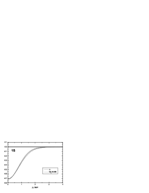
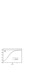
Figure 2: Profiles of decay matrix elements, Eq.(3) (scalar parts), for $1S(c\bar{c})$ into $DD$ (left panel) and $1S(b\bar{b})$ into $BB$ (right panel) calculated with decay vertex of Eq. (2), expression (12) – solid line, and for the constant decay vertex, expression (14) – broken line.

Surprisingly, that for the $nS$ bottomonium states the constant decay vertex reproduces results with the kernel $\mathcal{M}$ very well even for $4S$ and $5S$ states, however constants are different for different bottomonium states: $M_{\omega}$ varies from 0.65 GeV for $1S$ state to 1.3 GeV for $5S$ state (see right parts of Figs. 2,3,4,5,6), what we see in the case of charmonium states too.

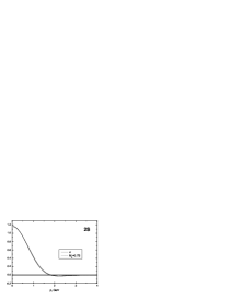
Figure 3: The same as in Fig. 2, but for the $2S(c\bar{c})$ into $DD$ (left panel) and $2S(b\bar{b})$ into $BB$ (right panel).

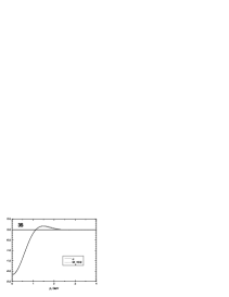
Figure 4: The same as in Fig. 2, but for the $3S(c\bar{c})$ into $DD$ (left panel) and $3S(b\bar{b})$ into $BB$ (right panel).

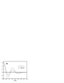
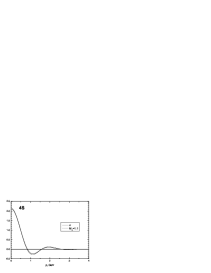
Figure 5: The same as in Fig. 2, but for the $4S(c\bar{c})$ into $DD$ (left panel) and $4S(b\bar{b})$ into $BB$ (right panel).

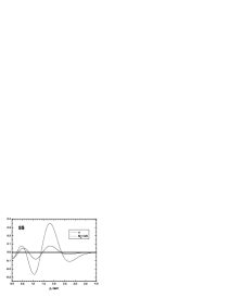
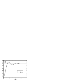
Figure 6: The same as in Fig. 2, but for the $5S(c\bar{c})$ into $DD$ (left panel) and $5S(b\bar{b})$ into $BB$ (right panel).

4 Analytic and phenomenological study of unquenched spectra

Our RSH was derived in Ref. [5] starting from the Wilson loop for the $q\bar{q}$ system and using Nambu-Goto action for the corresponding string. In the derivation presence of additional quark loops was neglected (quenched approximation), basing on the $1/N_{c}$ argument and additional (phenomenological) numerical suppression of the quark-loop effects. It is the purpose of the present Section to study these effects analytically and phenomenologically, and compare them with lattice results in the forthcoming Section.

The generating functional of heavy charges $Q\bar{Q}$, after integrating over other quark-loops, has the form

$$Z=\int DA\exp\ \mathcal{L}_{A}W_{Q\bar{Q}}(A)\det(m_{q}+\hat{D}(A)),$$ (15)

where $\mathcal{L}_{A}$ is the standard gluonic action and $W_{Q\bar{Q}}(A)$ is the external (fixed) Wilson loop of heavy quarks. The $\det$ term can be written in the path integral form [24]:

$$\det(m_{q}+\hat{D}(A))=\exp\left[tr\ln\left(\frac{1}{2}\int^{\infty}_{0}\frac{ds}{s}(D^{4}z)e^{-K}W_{q\bar{q}}(A)\right)\right],$$ (16)

where $(D^{4}z)$ is the path integration, $s$ is the proper time variable, $K=\frac{1}{4}\int^{s}_{0}\left(\frac{dz_{\mu}(\tau)}{d\tau}\right)^{2}d\tau$, and $W_{q\bar{q}}(A)$ is the Wilson loop of sea quarks, while $tr$ implies summation over flavor indices and space-time coordinates.

Expanding in the number of sea-quark loops, one has the first correction term [24]:

$$Z_{\rm 1loop}=\int DA\exp\mathcal{L}_{A}\left(\frac{1}{2}tr\left\{\int^{\infty}_{0}\frac{ds}{s}D^{4}z)e^{-K}W_{q\bar{q}}(A)W_{Q\bar{Q}}(A)\right\}\right).$$ (17)

Integrating in (17) over $DA$, one obtains the effective one-loop partition function,

$$Z_{\rm 1loop}=-\frac{1}{2}\int^{\infty}_{0}\frac{ds}{s}(D^{4}z)e^{-K}\chi(W_{q\bar{q}},W_{Q\bar{Q}}),$$ (18)

where $\chi$ is connected average of two loops,

$$\chi\equiv\langle W_{q\bar{q}}(A)W_{Q\bar{Q}}(A)\rangle-\langle W_{q\bar{q}}(A)\rangle\langle W_{Q\bar{Q}}(A)\rangle.$$ (19)

Properties of $\chi$ were studied in [25, 26], where it was shown that one can find a simple expression for $\chi$ for small distances between minimal area surfaces of both Wilson loops,

$$\chi\cong\frac{1}{N_{c}^{2}}\exp(-\sigma S_{\Delta})$$ (20)

and $S_{\Delta}$ is the minimal area of the surface connecting contours $C_{1}$ and $C_{2}$ of Wilson loops $W_{Q\bar{Q}}$ and $W_{q\bar{q}}$, respectively, as shown in Fig.7 One can see in Fig.7 that the width of the bands in $S_{\Delta}$ along time direction is of the order of $R_{2},R_{3}$, where $R_{2},R_{3}$ are the radii of intermediate mesons $(Q\bar{q})$ and $(\bar{Q}q)$.

Figure 7: Connected average of two Wilson loops, expressed via area law for the surface $S_{\Delta}$ between two loops. Radii $R_{2}$ and $R_{3}$ of two intermediate mesons $(Q\bar{q})$ and $(\bar{Q}q)$ are also shown.

Several properties of the effective partition function (18) can be derived immediately:

1) The general property of the unquenching process: since the integral $\int\frac{ds}{s}$ is obviously diverging at small $s$, one needs a renormalization step, which means that the string tension $\sigma$ in (20) is the renormalized (by unquenching) version of the quenched $\sigma$.

Expanding averaged static Wilson loop with sea quarks, one obtains

$$\langle W_{Q\bar{Q}|q\bar{q}}\rangle=\langle W_{Q\bar{Q}}\rangle+\frac{1}{N_{c}}\langle\langle W_{Q\bar{Q}}\bar{W}_{q\bar{q}}\rangle\rangle+\frac{1}{N^{2}_{c}}\langle\langle W_{Q\bar{Q}}\bar{W}_{q\bar{q}}\bar{W}_{q\bar{q}}\rangle\rangle+...,$$ (21)

where the bar over $W_{q\bar{q}}$ implies averaging over all paths, i.e. all contours of light quarks $C_{q\bar{q}}$ with the weight defined by the Fock-Feynman-Schwinger path integral,

$$\bar{W}_{q\bar{q}}=\int^{\infty}_{s_{0}}\frac{ds}{s}(D^{4}z)e^{-K}W_{q\bar{q}}(C_{q\bar{q}}).$$ (22)

Correspondingly, one can write each Wilson loop and their products as (omitting correction terms independent of $T$).

$$\langle W_{Q\bar{Q}}\rangle=\exp(-V_{Q\bar{Q}}(R)T)$$ (23)

$$\langle W_{Q\bar{Q}}\bar{W}_{q\bar{q}}\rangle\rangle=\exp(-V_{\Delta}(R)T);$$ (24)

$$\langle W_{Q\bar{Q}}\bar{W}_{q\bar{q}}\bar{W}_{q\bar{q}}\rangle\rangle=\exp(-V_{\Delta\Delta}(R)T).$$ (25)

Therefore the resulting $Q\bar{Q}$ interaction appears to be dependent on $T$. Since $V_{Q\bar{Q}}(R)=\sigma_{\rm ren}R+V_{\rm GE}(R)$, while $V_{\Delta\Delta}(R)<V_{\Delta}(R)<V_{Q\bar{Q}}(R)$ for large enough $R$, with increasing $T$ the $Q\bar{Q}$ system will pass from the purely confining regime $V_{Q\bar{Q}}$ to one-loop regime $V_{\Delta}$ and then to two-loop regime $V_{\Delta\Delta}$ etc. In the next Section we shall show that this type of transition was indeed observed on the lattice.

As to the form of $V_{\Delta}(R),V_{\Delta\Delta}(R)$ etc., one expects that for $R<R_{2}+R_{3}$, where $R_{2},R_{3}$ are radii of lowest $(Q\bar{q}),(\bar{Q}q)$ states, the form of $V_{\Delta}(R)$ does not change, i.e.

$$V_{\Delta}(R)\approx\sigma_{\rm ren}R,~{}~{}R<R_{2}+R_{3}\approx 1{\rm fm}.$$ (26)

In case of the $c\bar{c}$ system $R_{2}=R_{3}=R_{D}\approx R_{D^{*}}\approx 0.6$ fm. The same is true for $b\bar{b}$ system with $R_{B}\approx 0.5$ fm.

In a similar way one can treat $V_{\Delta\Delta}$ and higher loop terms. As a result one can predict that the static potential can be defined from the sum (21) in the $T$- independent way for $R\mathrel{\mathchoice{\lower 3.6pt\vbox{\halign{$\mathsurround=0pt\displaystyle\hfil#\hfil$\cr<\crcr\sim\crcr}}}{\lower 3.6pt\vbox{\halign{$\mathsurround=0pt\textstyle\hfil#\hfil$\cr<\crcr\sim\crcr}}}{\lower 3.6pt\vbox{\halign{$\mathsurround=0pt\scriptstyle\hfil#\hfil$\cr<\crcr\sim\crcr}}}{\lower 3.6pt\vbox{\halign{$\mathsurround=0pt\scriptscriptstyle\hfil#\hfil$\cr<\crcr\sim\crcr}}}}1$ fm,

$$V_{\rm static}(R)\approx V_{Q\bar{Q}}(R)\approx\sigma_{\rm ren}R,~{}~{}R\mathrel{\mathchoice{\lower 3.6pt\vbox{\halign{$\mathsurround=0pt\displaystyle\hfil#\hfil$\cr<\crcr\sim\crcr}}}{\lower 3.6pt\vbox{\halign{$\mathsurround=0pt\textstyle\hfil#\hfil$\cr<\crcr\sim\crcr}}}{\lower 3.6pt\vbox{\halign{$\mathsurround=0pt\scriptstyle\hfil#\hfil$\cr<\crcr\sim\crcr}}}{\lower 3.6pt\vbox{\halign{$\mathsurround=0pt\scriptscriptstyle\hfil#\hfil$\cr<\crcr\sim\crcr}}}}1{\rm fm}.$$ (27)

For $R>1.2$ fm the situation is complicated and static $(T$-independent) potential cannot be defined in the strict sense, as was discussed above. In this case another approach can be used, namely, the expansion of the connected averages $\langle\langle W_{Q\bar{Q}}\bar{W}_{q\bar{q}}\rangle\rangle$ in the series over intermediate heavy-light meson states, as was done in [18], and it is equivalent to the expansions in [4], [17], [20, 21, 22, 23]. In this way instead of $V_{\Delta}(R)$ one defines the energy-dependent nonlocal interaction

$$V_{121}(\mbox{\boldmath${\rm q}$},\mbox{\boldmath${\rm q}$}^{\prime},E)=\sum_{n_{2}n_{3}}\int\frac{d^{3}\mbox{\boldmath${\rm p}$}}{(2\pi)^{3}}\frac{X_{n_{2}n_{3}}(\mbox{\boldmath${\rm q}$}-\mbox{\boldmath${\rm p}$})X^{+}_{n_{2}n_{3}}(\mbox{\boldmath${\rm q}$}^{\prime}-\mbox{\boldmath${\rm p}$})}{E-E_{n_{2}n_{3}}(\mbox{\boldmath${\rm p}$})},$$ (28)

where subscripts 1,2 refer to the channels $Q\bar{Q}$ and $(Q\bar{q})(\bar{Q}q)$, respectively, while $n_{2},n_{3}$ are quantum numbers of the mesons $(Q\bar{q})$ and $(\bar{Q}q)$ with the wave functions $\psi_{n_{2}}$ and $\psi_{n_{3}}$, and

$$X_{n_{2}n_{3}}(\mbox{\boldmath${\rm r}$})=\frac{M_{\omega}\eta(\beta,\gamma)}{\sqrt{N_{c}}}\int\frac{d^{3}\mbox{\boldmath${\rm q}$}}{(2\pi)^{3}}e^{i\mbox{\boldmath${\rm q}$}\mbox{\boldmath${\rm r}$}}\psi_{n_{2}}(\mbox{\boldmath${\rm q}$})\psi_{n_{3}}(\mbox{\boldmath${\rm q}$}).$$ (29)

In a similar way instead of $V_{\Delta\Delta}(R)$, one defines the interaction $V_{131}$ due to three-meson intermediate states.

As a result, the total Hamiltonian has the form

$$H=H_{kin}+V_{Q\bar{Q}}(\mbox{\boldmath${\rm R}$})+V_{121}(\mbox{\boldmath${\rm R}$},\mbox{\boldmath${\rm R}$}^{\prime},E)+V_{131}(\mbox{\boldmath${\rm R}$},\mbox{\boldmath${\rm R}$}^{\prime},E)+....$$ (30)

As one can see, in (30) the $T$-dependent interaction of (23), (24), (25) is replaced by the energy-dependent nonlocal interaction.

Let us underline general properties of the new Hamiltonian (for an earlier discussion see [34]).

i) For energies below all thresholds the interaction $\sum_{n\geq 2}V_{1n1}(\mbox{\boldmath${\rm R}$},\mbox{\boldmath${\rm R}$},E)$ is negative, which implies attraction on average from all higher intermediate states. Hence the linear potential in $V_{Q\bar{Q}}(R)$ is modified (flattened) by inclusion of intermediate states. This attraction also persists in some energy region above thresholds, where the real part of $V_{1n1}$ is still negative.

ii) Due to strong reduction of overlap integrals of the type $||\Psi_{k}(\mbox{\boldmath${\rm R}$})V_{1n1}$ $(\mbox{\boldmath${\rm R}$},\mbox{\boldmath${\rm R}$}^{\prime},E)\Psi_{l}(\mbox{\boldmath${\rm R}$}^{\prime})||$ (as was discussed in previous Section, it is due to the string width effect), the series $\sum_{n\geq 2}V_{1n1}$ is fast converging and therefore only few terms are important.

Summarizing the effect of sea-quark loop on the $Q\bar{Q}$ interaction, one can say that there is no energy-independent (or time-independent) universal local interaction which can describe the dynamics of $Q\bar{Q}$ system in the unquenched case. If one tries to simulate the effect of quark loops on the static $Q\bar{Q}$ potential, then it should be an approximate local interaction, which is close to linear potential $\sigma_{\rm ren}R$ for $R\mathrel{\mathchoice{\lower 3.6pt\vbox{\halign{$\mathsurround=0pt\displaystyle\hfil#\hfil$\cr<\crcr\sim\crcr}}}{\lower 3.6pt\vbox{\halign{$\mathsurround=0pt\textstyle\hfil#\hfil$\cr<\crcr\sim\crcr}}}{\lower 3.6pt\vbox{\halign{$\mathsurround=0pt\scriptstyle\hfil#\hfil$\cr<\crcr\sim\crcr}}}{\lower 3.6pt\vbox{\halign{$\mathsurround=0pt\scriptscriptstyle\hfil#\hfil$\cr<\crcr\sim\crcr}}}}1$ fm, and becomes softer (flattening) for larger $R$, which can be approximated by making $\sigma_{\rm ren}$ the energy – and $R$ -dependent.

Such kind of flattening potential was introduced in [15] to describe high excitations of light mesons and used latter in [12, 13, 14] for higher charmonium states.

$$\tilde{V}_{Q\bar{Q}}(R)=\sigma(R)\cdot R;~{}~{}\sigma(R)=\sigma_{0}\left[1-\gamma_{0}\frac{\exp(\sqrt{\sigma_{0}}(r-R_{1}))}{B+\exp(\sqrt{\sigma_{0}}(r-R_{1}))}\right].$$ (31)

Here $R_{1}\approx 1.2$ fm is the distance, where the string can decay into two mesons, $\sigma_{0}R_{1}+2M_{Q}\approx 2M_{Q\bar{q}},\sigma_{0}=0.19$ GeV². Putting $\gamma_{0}=0.40$, the best description of radial excited light mesons was obtained in [15]. The modified potential $\tilde{V}_{Q\bar{Q}}(R)$, taken from [15], is shown in Fig.8.

Figure 8: Modified potential with parameters given in Eq. (31). For reference simple linear potential with $\sigma=0.19$ GeV² is also plotted.

The resulting light meson masses, taken from [15], are compared with experimental data in Table 1. For heavy quarkonia the role of the flattening is less important. Below in Table 2 one can see corresponding effect in charmonium levels, which is of the order of several tens of MeV for high excitations.

Another types of flattening potentials were suggested in [35]. One should, however, be careful with the large $R$ behavior of their flattening potentials, which is bounded from above, and therefore the quarks $Q,\bar{Q}$ can liberate themselves and this effect contradicts the physical picture in QCD, when an unstable hadron decays into hadrons, but not into quarks.

Table 1: Light meson masses $M_{0}(nL)$ (in GeV) from RSH with pure linear potential and their masses $\tilde{M}_{0}(nL)$ in potential with flattening. The corresponding flattening correction $\delta_{\rm flat}$ (in MeV), the self-energy correction $\Delta_{SE}=-\frac{12\sigma}{\pi M_{0}}$, the string correction $\Delta_{str}=\frac{2\sigma\langle r^{-1}\rangle l(l+1)}{M^{2}_{0}}$, and the resulting mass $M_{tot}=\tilde{M}_{0}+\delta_{SE}+\Delta_{str}+\delta_{GE}$ (where $\delta_{GE}$ is the correction from the gluon-exchange potential) are given in GeV.

State	$\gamma=0$	$\gamma=0.4$	$\delta_{\rm flat}$ (MeV)	$\Delta_{SE}$	$\Delta_{str}$	$M=\tilde{M}_{0}$
nL	$M_{0}(nL)$	$M_{0}(nL)$	flattening
1S	1.347	1.335	-12	-0.510	0	$0.725$
2S	2.009	1.944	-65	-0.342	0	$1.503$
1D	2.167	2.122	-45	-0317	-0.087	1.662
3S	2.512	2.300	-212	-0.274	0	1.937
2D	2.615	2.428	-187	-0.263	-0.058	2.052
4S	2.931	2.569	-362	-0.235	0	2.252
3D	3.006	2.647	-359	-0.229	-0.043	2.322
1P	1.802	1.777	-25	-0.382	-0.074	0.071
2P	2.328	2.213	-115	-0.295	-0.030	0.068
1F	2.479	2.402	-77	-0.277	-0.113	0.048
3P	2.766	2.472	-294	-0.249	-0.020	0.065
2F	2.876	2.606	-270	-0.239	-0.083	0.047
4P	3.146	2.731	-415	-0.219	-0.015	0.062
3F	3.233	2.821	-412	-0.213	-0.064	0.046

Table 2: Comparison of the single-channel and flattening potential results for S,P,D states of charmonium with existing experimental data.

State	SC	flattening	exp
1S	3.068	3.066	3.067
2S	3.678	3670	3.74(4)
3S	4.116	4.093	$4.040(3^{3}S_{1})$
4S	4.482	4.424	$4.421(4^{3}S_{1})$
5S	4.806	4.670	?
1P	3.488	3.484	3.525 $(^{1}P_{1})$
2P	3.954	3.940	$\sim 3.93(^{5}P_{2})$
3P	4.338	4.299	-
1D	3.79	3.78	$3.77(1^{3}D_{1})$
2D	4.189	4.165	4.153(3)
3D	4537	4.475	-

5 Comparison to other approaches

Here we compare our string decay picture with lattice data and other approaches. On the lattice the topic of string breaking and $Q\bar{Q}$ interaction above inelastic threshold was actively explored during last decade (for the first attempts see [36] and [37]). A way to determine the static potential in unquenched case was suggested in [38] and several spectra calculations, including sea-quark effects, were done in [39]. Recently careful studies of spectra of excited hadrons with open channels were published in [40] and [41], where the importance of inelastic channels was stressed. The difficulty of existing lattice approaches is the lack of the proper definition of a resonance state, which actually belongs to the continuous spectrum and requires either the continuous density description or the use of the Weinberg Eigenvalue Method, described recently in the last paper of Ref. [19]. The first approach is made possible by the use of the finite volume, when continuous states are discretized and the resonance is defined by the scattering phase [36, 37]. The second approach, to our knowledge, was never used on the lattice. As to precise definition of the resonance parameters on the lattice, from [40, 41] one can see that it needs a lot of efforts and is expected in the nearest future.

It is worth saying that the $Q\bar{Q}$ potential, calculated on the lattice, is not sensitive to the effects of the virtual sea quarks at least for distances $R\mathrel{\mathchoice{\lower 3.6pt\vbox{\halign{$\mathsurround=0pt\displaystyle\hfil#\hfil$\cr<\crcr\sim\crcr}}}{\lower 3.6pt\vbox{\halign{$\mathsurround=0pt\textstyle\hfil#\hfil$\cr<\crcr\sim\crcr}}}{\lower 3.6pt\vbox{\halign{$\mathsurround=0pt\scriptstyle\hfil#\hfil$\cr<\crcr\sim\crcr}}}{\lower 3.6pt\vbox{\halign{$\mathsurround=0pt\scriptscriptstyle\hfil#\hfil$\cr<\crcr\sim\crcr}}}}1$ fm (for the latest calculation see [42]). This result is in agreement with our discussion of the structure of the unquenched Wilson loop in the previous Section.

Table 3: Comparison of calculated mass $M_{tot}$ (in GeV) with experimental data.

$M_{tot}$	Theory	Exp.	$M_{cog}(th)$
$M(\rho(1S))$	0.749	$\rho(0.775)$	0.666
$M(\rho(2S))$	1.519	$\rho(1.465)$	1.479
$M(\rho(3S))$	1.937	$\rho(1900)?$	1.849
$M(\rho(4S))$	2.252	$\rho(2150)?$	2.166
$\bar{M}(1P)$	1.25	$a_{1}(1230)$
		$f_{1}(1282)$
$\bar{M}(2P)$	1.82	$a_{1}(1647)?a_{2}(1732)?$
		$f_{1}(1815)?$
$\bar{M}(3P)$	2.14	$f_{2}(2157)$ mixing for $3^{3}P_{2}$
$\bar{M}(4P)$	2.435		1.65
$\bar{M}(1D)$	1.66	$\rho_{3}(1690),\rho(1720)$
		mixing for $2^{3}S_{1}-1^{3}D_{1}$
$\bar{M}(2D)$	2.05	$\rho_{3}(1990)?$	1.989
$\bar{M}(3D)$	2.32	$\rho_{3}(2250)?,\rho_{5}(2330)?$	2.249
		$(3D-2G$ mixing(?))
$\bar{M}(1F)$	1.96	$a_{4}(2000),f_{4}(2018)$
$\bar{M}(2F)$	2.24	$f_{4}(2300)$
$\bar{M}(3F)$	2.50

References

- [1] J. M. Richard, Phys. Lett. B 100, 515 (1980); ibid 95, 299 (1980); D. P. Stanley and D. Robson, Phys. Rev. Lett. 45, 235 (1980); Phys. Rev. D 21, 3180 (1980); P. Cea, G. Nardulli, and G. Preparata, Z.Phys. C 16, 135 (1982); J. Carlson, J. Kogut, and V. R. Pandharipande, Phys. Rev. D 27, 233 (1983); J. L. Basdevant and S.Boukraa, Z. Phys. C 28, 413 (1983).
- [2] N. Isgur and S. Godfry, Phys. Rev. D 32, 189 (1985).
- [3] S. Capstick and N. Isgur, Phys. Rev. D 34, 2809 (1986).
- [4] E. Eichten, K. Gottfried, T. Kinoshita, K. D. Lane, and T. M. Yan, Phys. Rev. D 17, 3090 (1978) (Erratum:ibid. D 21, 313 (1980)), ibid. D 21, 203 (1980); Phys. Rev. Lett. 36, 500 (1976).
- [5] A. Yu. Dubin, A. B. Kaidalov, and Yu. A. Simonov, Phys. Lett. B 323, 41 (1994); Phys. At. Nucl. 56, 1745 (1993); Nuovo Cim. A 107, 2499 (1994); E. L. Gubankova and A. Yu. Dubin, Phys. Lett. B 334, 180 (1994).
- [6] Yu. A. Simonov, in “QCD: Perturbative or Nonperturbative ?” Ed. by L. Ferreira, P. Nogueira, and J. I. Silva-Marcos ( World Sci., Singapore (2001), p.60; arXiv: hep-ph/9911237.
- [7] Yu. S. Kalashnikova, A. V. Nefediev, and Yu. A. Simonov, Phys.Rev. D 64, 014037 (2001).
- [8] Yu. A. Simonov, Phys. Lett. B 515, 137 (2001); A. Di Giacomo and Yu. A. Simonov, Phys. Lett. B 595, 368 (2004).
- [9] A. M. Badalian and B. L. G. Bakker, Phys. Rev. D 66, 034025 (2002).
- [10] V. L. Morgunov, A. V. Nefediev, and Yu. A. Simonov, Phys. Lett. B 459, 653 (1999).
- [11] Yu. A. Simonov and V. I. Shevchenko, Adv. High Energy, 2009, 873051 (2009); arXiv: 0902.1405 [hep-ph]; Yu. A. Simonov, arXiv: 1003.3608 [hep-ph].
- [12] A. M. Badalian, Phys. At. Nucl. 74, 1375 (2011); arXiv: 1011.5580 [hep-ph].
- [13] A. M. Badalian, B. L. G. Bakker, and I. V. Danilkin, Phys. Rev. D 81, 071502 (2010).
- [14] A. M. Badalian and B. L. G. Bakker, Phys. Rev. D 84, 034006 (2011); A. M. Badalian, B. L. G. Bakker, and I. V. Danilkin, Phys. At. Nucl. 74, 631 (2011).
- [15] A. M. Badalian, Phys. At. Nucl. 66, 1342 (2003); A. M. Badalian, B. L. G. Bakker, and Yu. A. Simonov, Phys. Rev. D 66, 034006 (2002).
- [16] S. M. Fedorov and Yu. A. Simonov, JETP Lett. 78, 57 (2003); hep-ph/0306216 [hep-ph].
- [17] E. van Beveren, C. Dullemond, and G. Rupp, Phys. Rev. D 21, 772 (1980), E. van Beveren, Z.Phys. C 17, 135 (1983); E. van Beveren, G. Rupp, T. A. Rijken, and C. Dullemond, Phys. Rev D 27, 1527 (1983); S. Jacobs, K. J. Miller, and M. G. Olsson, Phys. Rev. Lett. 50, 1181 (1983); G. Fogli and G. Preparata, Nuovo Cimento, A 48, 235 (1978); A. C. Maciel and J. Paton, Nucl. Phys. B 181, 277 (1981); N. A. Törnqvist, Ann. Phys. (N.Y.) 135, 1 (1978); M. Ross and N. A. Törnqvist, Z. Phys. C 5, 205 (1980), N. A. Törnqvist, Phys. Rev. Lett. 49, 624 (1982); Nucl. Phys. B 203, 268 (1982).
- [18] Yu. A. Simonov, Phys. At. Nucl. 71, 1048 (2008), arXiv;0711.3626; Yu. A. Simonov, A. I. Veselov, Phys. Rev. D 79, 034024 (2009); I. V. Danilkin and Yu. A.‘Simonov, Phys. Rev. D 81, 074027 (2010).
- [19] L. Micu, Nucl. Phys. B 10, 521 (1969); A. Le Yaouanc, L. Olivier, O. Pene, and J. Raynal, Phys. Rev. D 8, 2223 (1973); ibid. D 9, 1415 (1974); D 11, 1272 (1975); D 21, 182 (1980).
- [20] N. Isgur and J. Paton, Phys. Rev. D 31, 2910 (1985); H. Blundell and S. Godfrey, Phys. Rev. D 53, 3700 (1996); T. Barnes, F. E. Close, P. R. Page, and E. S. Swanson, Phys. Rev. D 55, 4157 (1997); P. K. Page, Nucl. Phys. B 446, 189 (1995); P. Geiger and E. S. Swanson, Phys. Rev. D 50, 6855 (1994); H. Q. Zhou, R. G. Ping, and B. S. Zou, Phys. Lett. B 611, 123 (2005); X. H. Guo, H. W. Ke, X. Q. Li, X. Liu, and S. M. Zhao, Commun. Theor. Phys. 48, 509 (2007); J. Lu, W. Z. Deng, X. L. Chen, and S. L. Zhu, Phys. Rev. D 73, 054012 (2006).
- [21] E. S. Ackleh, T. Barnes, and E. S. Swanson, Phys. Rev. D 54, 6811 (1996).
- [22] K. Heikkilá, N. A. Törnqvist, and S. Oho, Phys. Rev. D 29, 110 (1984); Yu. S. Kalashnikova, Phys. Rev. D 72, 034010 (2005); M. K. Pennington and D. J. Wilson, Phys. Rev. D 76, 077502 (2007); T. Barnes and E. S. Swanson, Phys. Rev. C 77, 055206 (2008); S. Godfrey and R. Kokoski, Phys. Rev. D 43, 1679 (1991); F. E. Close and E. S. Swanson, Phys. Rev. D 72, 094004 (2005); E. S. Swanson, J. Phys. G 31, 845 (2005); D. S. Hwang and D. W. Kim, Phys. Lett. B 601, 137 (2004); E. J. Eichten, K. Lane, and C. Quigg, Phys. Rev. D 69, 094019 (2004); C. Hanhart, Yu. S. Kalashnikova, A. E. Kudryavtsev, and A. V. Nefediev, Phys. Rev. D 76, 034007 (2007); Yu. S. Kalashnikova, AIP Conf. Proc. 892, 318 (2007); Yu. S. Kalashnikova, Phys. Rev. D 72, 034010 (2005); C. Amsler and N. A. Törnqvist, Phys. Rept. 389, 61 (2004).
- [23] P. Geiger and N. Isgur, Phys. Rev. D 41, 1595 (1990), ibid D 44, 799 (1991), ibid D 47, 5050 (1993).
- [24] Yu. A. Simonov, Phys. Rev. D 84, 065013 (2011).
- [25] Yu. A. Simonov, Phys. Usp. 39, 313 (1996), [hep-ph/9709344]; D. S. Kuzmenko, V. I. Shevchenko, and Yu. A. Simonov, Phys. Usp. 104, 3 (2004).
- [26] L. Del Debbio, A. Di Giacomo, and Yu. A. Simonov, Phys. Lett. B 332, 111 (1994); N. Cardoso, M. Cardoso, and P. Bicudo, Phys. Lett. B 710, 343 (2012).
- [27] R. W. Haymaker, V. Singh, Y. Peng, and J. Woisiek, Phys. Rev. D 53, 389 (1996); P. Bicudo, N. Cardoso, and M. Cardoso, arXiv: 1010.3870.
- [28] H. G. Dosch, Phys. Lett. B 190, 177 (1987); H. G. Dosch and Yu. A. Simonov, Phys. Lett. B 205, 339 (1988); A. Di Giacomo, H. G. Dosch, V. I. Shevchenko, and Yu.A.Simonov, Phys. Rept. 372, 319 (2002).
- [29] G. S. Bali, N. Brambilla, and A. Vairo, Phys. Lett. B 421, 265 (1998); Y. Koma, M. Koma, Nucl. Phys. B 769, 79 (2007).
- [30] Yu. A. Simonov, Phys. At. Nucl. 71, 1048 (2008); Yu. A. Simonov and A. I. Veselov, Phys. Rev. D 79, 034024 (2009).
- [31] Yu. A. Simonov and A. I. Veselov, Phys. Lett. B671, 55 (2009).
- [32] I. V. Danilkin, V. D. Orlovsky, and Yu. A. Simonov, Phys. Rev. D 85, 034012 (2012).
- [33] T. Barnes, S. Godfrey, and E. S. Swanson, Phys. Rev. D 72, 054026 (2005).
- [34] A. M. Badalian, L. P. Kok, M. I. Polikarpov, and Yu. A. Simonov, Phys. Rept. 82, 31 (1982).
- [35] Y. B. Ding, K. T. Chao, and D. H. Qin, Chin. Phys. Lett. 10, 460 (1993); Phys. Rev. D 51, 5064 (1995); B. Q. Li, C. Meng, and K. T. Chao, Phys. Rev. D 80, 014012 (2009).
- [36] M. Lüscher, Comm. Math.Phys. 104, 177 (1986); ibid 105, 153 (1986); Nucl. Phys. B 354, 531 (1991); ibid. B 364, 237 (1991).
- [37] C. Mc Neil and C. Michael (UKQCD), Phys. Lett. B 556, 177 (2003); C. Michael, Eur. Phys. J. A 31, 793 (2007); Z. Prkacin, G. S. Bali, Th.Düssel et al, PoS LATTICE2005, 308 (2005) [hep-lat/0510051].
- [38] M. Donnellan, F. Knechtli, B. Leder, and R. Sommer, Nucl. Phys. D 849, 45 (2011).
- [39] T. Burch et al. [Fermilab Lattice and MILC Collab.], Phys. Rev. D 81, 034508 (2010); E. Follana et al. [HPQCD and UKQCD Collab.], Phys. Rev. D 75, 054502 (2007); Y. Namekawa et al. [PACS-CS Collab.], PoS LATTICE2008, 121 (2008); Y. Namekawa et al. [PACS-CS Collaboration], Phys. Rev. D 84, 074505 (2011); G. S. Bali et al., PoS LATTICE2011, 135 (2011); S. M. Ryan [Hadron Spectrum Collab.], PoS LATTICE2010, 124 (2010).
- [40] G. S. Bali, S. Collins, and C. Ehmann, Phys. Rev. D 84, 094506 (2011).
- [41] C. Morningstar et al., AIP Conf. Proc. 1441, 290 (2012); arXiv:09.0308 [hep-lat].
- [42] T. Kawanai and S. Sasaki [Tokyo U., RIKEN BNL, and Brookhaven Collab.], Phys. Rev. D 85, 091503 (2012).