Turbulence in weakly-ionized proto-planetary disks
Abstract
We investigate the characteristic properties of self-sustained MRI turbulence in low-ionized proto-planetary disks. We study the transition regime between active and dead-zone, performing 3D global non-ideal MHD simulations of stratified disk covering range of magnetic Reynolds number between . We found converged and saturated MRI turbulence for with a strength of . Below the MRI starts to decay at the midplane, having Elsasser numbers below one. We find a transition regime between where the MRI turbulence is still sustained but damped. At around the MRI turbulence decays but could reestablished due to the accumulation of toroidal magnetic field or the radial transport of magnetic field from the active region. Below the MRI cannot be sustained and is decaying. Here hydro-dynamical motions, like density waves dominate. We observe long-living anti-cyclonic vortices in the transition between dead-zone and active zone.
1 Introduction
The magneto-rotational instability (MRI) is a
candidate for driving turbulence and enabling the accretion of matter onto the central object
(Balbus & Hawley, 1991, 1998; Hawley & Balbus, 1991). Dependent on the ionization
degree, the MRI generated turbulence will be reduced, down to a low
turbulence regime, called the dead zone
(Blaes & Balbus, 1994; Jin, 1996; Sano et al., 2000). Various studies showed that a
certain level of resistivity suppresses MRI activity (Fleming et al., 2000; Sano & Stone, 2002a, b; Fleming & Stone, 2003; Inutsuka & Sano, 2005; Turner et al., 2007, 2010; Turner & Sano, 2008).
One of the most important dimensionless number, characterizing the coupling between gas and magnetic fields,
is the magnetic Reynolds number which
relates the timescale of magnetic advection to magnetic diffusion. We consider here the Ohmic diffusion term which is most important at the midplane.
Up to now, there is no clear prescription for which values of the
MRI turbulence is sustained in disks. Fleming et al. (2000) found sustained MRI with a zero-net flux magnetic field for
.
A recent study by Simon et al. (2011), using stratified local box simulations,
investigate the turbulence level for different values of the magnetic
Reynolds and Prandtl number. They found a so-called low state, a state where
turbulence is partly suppressed, but sustained due to a dynamo process.
In addition, they predict a critical Reynolds numbers in the range between . A similar region was investigated by Oishi & Mac Low (2011) in which they found . This critical Reynolds number is important to model the surface density of active layers in proto-planetary disk as it was recently done by
Martin et al. (2012).
In our study, we will search for the critical magnetic Reynolds number in global zero-net flux stratified MRI simulations. Here the MRI turbulence criterion, Elsasser number , should become unity. In contrast to the magnetic Reynolds number, the Elsasser number gives one clear threshold independent of the magnetic geometry or the stratification. We will also investigate the hydrodynamical motions which become important in the dead-zone region (Oishi & Mac Low, 2009).
We concentrate on the magnetic Reynolds
number regime proposed by Simon et al. (2011) and Oishi & Mac Low (2011).
For our simulations we use only explicit resistivity.
Oishi & Mac Low (2011) found out that well ionized MRI turbulence scales independently of if .
In addition, as the molecular viscosity is very small in proto-planetary disks we expect Prandtl numbers of and we focus on this low Prandtl number regime 111Here the hydrodynamic viscosity is small compared to
the magnetic diffusivity .
In this paper we will first describe the numerical and physical setup. Then we will present the results, discussion and the conclusion.
2 Setup
The initial conditions for density, pressure and azimuthal velocity follow hydrostatic equilibrium. We set the density to
| (1) |
with , the scale height to radius , . The pressure follows locally an isothermal equation of state: with the sound speed . The azimuthal velocity is set to
| (2) |
The initial velocities and are set to a white noise perturbation amplitude of . We start the simulation with a pure toroidal magnetic seed field with constant plasma beta . To obtain a range of magnetic Reynolds number we keep the magnetic dissipation value constant in the disk. We use three different values of , , and .
| (3) |
To estimate the numerical magnetic Reynolds number having MRI turbulence simulations
we run also ideal MHD simulations with different resolutions as reference.
The radial domain extends from 1 to 10 AU.
The domain covers 4.3 disk scale heights, or .
For the azimuthal domain we use for the L models and for the H models.
We use a uniform grid in spherical coordinates.
Models L have a resolution of , , and for the H models.
All models resolve the radial scale height with 9 to 22 grid cells for the inner and outer radius. The vertical scale height is resolved by 22 grid points. In models L the azimuthal scale height is resolved by 9 grid cells. The H models have a higher resolution of 17 per scale height in the azimuth. Their are calculated with the FARGO MHD to reduce even more the numerical dissipation (Mignone et al., 2012). The simulation models are summarized in table 1. We note that model is special. Here the numerical dissipation cannot be neglected. By comparing with the results of H models,
the model shows magnetic Reynolds number below the value used in . This model establishes a large dead-zone region. Here hydro-dynamical motions become important.
| Model name | FARGO | Rm | ||
|---|---|---|---|---|
| xx | 1-10 : 0.6 : | NO | Ideal | |
| xx | 1-10 : 0.6 : | YES | Ideal | |
| xx | 1-10 : 0.6 : | YES | Ideal | |
| xx | 1-10 : 0.6 : | YES | 4300-6300 | |
| xx | 1-10 : 0.6 : | YES | 3300-4800 | |
| xx | 1-10 : 0.6 : | YES | 2700-4300 | |
| xx | 1-10 : 0.6 : | NO | 3000* |
Buffer zones extent from 1 to 2 AU as well as from 9 to 10 AU. In the buffer zones we use a linearly increasing resistivity (up to ) reaching the boundary. This damps the magnetic field fluctuations and suppresses boundary interactions. For our analysis we use the range between 3 and 8 AU, which is not affected by the buffer zones. Our outflow boundary condition projects the radial gradients in density, pressure and azimuthal velocity into the radial boundary and the vertical gradients in density and pressure at the boundary. For all runs we employ the second order scheme in the PLUTO code with the HLLD Riemann solver (Miyoshi & Kusano, 2005), piece-wise linear reconstruction and order Runge Kutta time integration. We treat the induction equation with the ”Constrained Transport” (CT) method in combination with the upwind CT method described in Gardiner & Stone (2005), using explicit resistivity. A more detailed description of the physical setup can be found in Flock et al. (2011).
3 Results
According to Eq. 3, we obtain a specific value of magnetic Reynolds number at each radius, resulting in a specific value of turbulence. To compare the results at different specific radii the timescale of radial mixing is important. Due to the low magnetic dissipation, the timescale of magnetic diffusion is very long compared to the turbulent mixing timescale. The maximum radial mixing scale for an alpha value of 0.01 after 1000 years at the outer radius at 8 AU is around . For our analysis we use specific radial positions which are separated enough. In chapter 3.5 we will investigate how the radial transport of magnetic field effects the local evolution. The value at a specific radial position is calculated with
| (4) |
The integral is done for each radius separately with and is the left and right radial cell boundary. The is mass weighted to recover the correct total value. In chapter 3.1 we compare results having the same local time period. Here we average , the turbulent velocities and the dynamo between 25 and 60 local orbits. This ensures that we compare the same dynamical evolution at a specific radius and Reynolds number. The space average of and is done at the midplane region between scale heights. In chapter 3.2 we concentrate on the longterm evolution for different values of . There we include the two MRI criteria, the Elsasser number
| (5) |
as well as the factor Q
| (6) |
The Q factor is the ratio of the MRI fastest-growing azimuthal wavelength to the azimuthal cell size. The value should be larger than 8 (Flock et al., 2010). In chapter 3.3 we concentrate on the run having the largest dead-zone. Here we present results of the dominant hydro-dynamical motions.
3.1 Time averaged statistics
Due to the change of the rotation period with radius, the comparison of the turbulence statistics at different radii is limited
to the number of rotations at the outer radius. We therefore present the comparison for the different Reynolds numbers
between a time average of local orbits. We note that in this period the initial net magnetic flux has already vanished and we have a zero-net flux MRI turbulence.
We note also that the results from model should be excluded. They indicate that here the explicit dissipation is not resolved and the numerical dissipation dominates.
We still overplot the results obtained by this lower resolution (L models, Fig. 1 blue color) to estimate the total magnetic Reynolds number. This model will be still useful as it shows very
similar conditions as present in dead-zones.
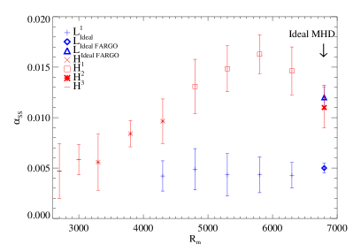
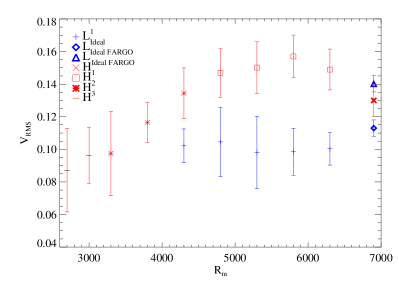
Fig. 1 combines the results of , the turbulent RMS velocity and the dynamo value as a function of the magnetic Reynolds number.
The results show for all turbulent quantities a saturation for magnetic Reynolds numbers around 5000 and above.
Below the MRI is damped and the turbulence decreases.
We observe a slightly higher turbulence level for high magnetic Reynolds numbers compared to fully ideal MHD run.
There is a saturation of at around value for magnetic Reynolds numbers greater than 5000, see Fig. 1 top.
Below , drops down to at around . Even one could see a flattening at around the values are still dominated by Maxwell stress which indicates that the MRI is still operating.
The turbulent velocity scales roughly with the square root of , found in recent local box simulations of dead-zones (Okuzumi & Hirose, 2011).
We observe a saturation around (Fig. 1, middle). Below , drops down to at around . We note again that these values represent the turbulent motions at the midplane, in the corona the turbulent velocity increases also in the dead-zone models.
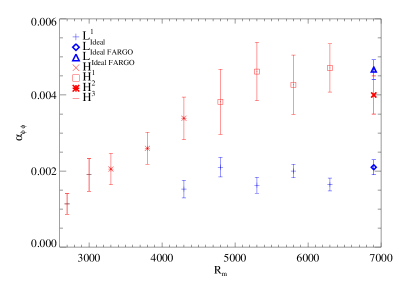
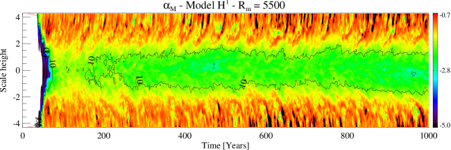
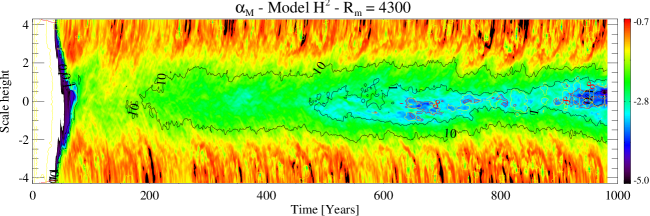
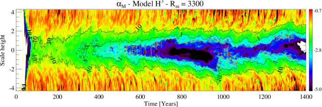
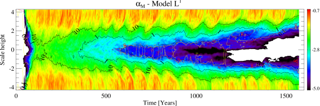
The dynamo action could be expressed by showing the correlations with
. We follow the analysis described in chapter 3.7 in (Flock et al., 2012) and
is normalized over . The dynamo action in the northern hemisphere is shown in Fig. 1, bottom. saturates at around 0.004 and decreases only down to 0.002 at .
In all runs the sign of in the southern hemisphere is negative with similar amplitude as the corresponding value in the northern hemisphere.
The results of the ideal MHD runs show convergence. Here the FARGO MHD method plays an important role in decreasing numerical dissipation as it is
presented in Mignone et al. 2012, A&A accepted. converge around 0.01.
We note again that the results presented in Fig. 1 reflect mainly the turbulence level at the midplane. In addition we see here no decay of the MRI turbulence due to the short time period.
In the next chapter we will concentrate on the longterm evolution over height for specific Reynolds number.
3.2 Longterm evolution
The previous chapter has shown the transition to saturated turbulence in well ionized disk regions.
In this chapter we focus on the longterm evolution, including the turbulence over height. For each model we perform the analysis at a specific Reynolds number which are located in the middle of the domain.
Here, has , for model and for model . In model we expect to have a Reynolds number around by comparison with model .
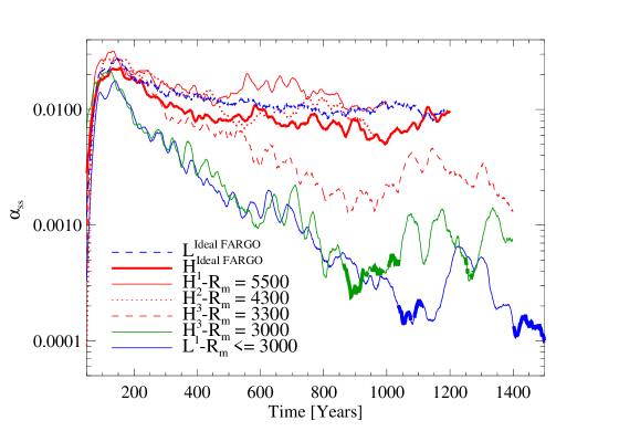
We plot the time evolution of in Fig. 2.
The analysis show that both ideal runs as well as the resistive runs down to ( and ),
show a steady turbulent evolution with .
The models and with show a steady decrease of the turbulence until they oscillate
in the range between . Due to the decrease we note that the results of the models and plotted in Fig. 1 depend on the averaged time period. For these models, an extended simulation runtime was needed.
We mark the regions with dominating Reynolds stress in thick (blue and green solid lines).
The plots show only a short-term domination which indicate that the total integral over height suggest still a operating MHD turbulence. The configuration of the Maxwell stress over height is presented in Fig. 3.
After around 200 inner orbits (years) the initial net azimuthal flux is lost and the flux start to oscillate around zero (Fromang & Nelson, 2006; Beckwith et al., 2011; Flock et al., 2011).
For a magnetic Reynolds number above the ionization is well enough to sustain the MRI turbulence at each height. In the midplane region we found
a saturation of at around . In model , Fig. 3, top, the Elsasser number is between 1 and 10 in the midplane region.
If the ionization is decreased below the Elsasser number reaches unity at the midplane (see also Fig. 4).
In model , Fig. 3, second from top, there is a small region at the midplane with . The total is still around 0.01 (compare Fig. 2)
but with higher fluctuations. Locally the magnetic turbulence starts to vanish at the midplane.
At around (model ) the total gets affected and decreases (compare Fig. 2).
In model the Elsasser number point is around 1 scale height. At the midplane drops below 0.1.
We confirmed the region equivalent with the definition by Okuzumi & Hirose (2011), Fig. 1 therein.
At this point also the azimuthal MRI wavelength becomes unresolved (, red solid line). At the midplane the Reynolds stress dominate over the Maxwell stress (Fig. 3, yellow solid line).
At , the MRI gets strongly damped. For model and model after around 500 years,
the poloidal magnetic fields decreases until the Elsasser number drops below 0.1 as well as the azimuthal MRI wavelength becomes unresolved (Fig. 3, red solid line). If the turbulence is able to survive depends also on the surrounding layers.
Even we choose a constant resistivity, the turbulence in the runs and is similar as they are present
in dead-zones. Turbulent upper layers of the disk are usually active (Turner & Sano, 2008; Dzyurkevich et al., 2010; Bai, 2011).
In this active layers the turbulent mixing is also stronger and active channels can reach into the dead-zone.
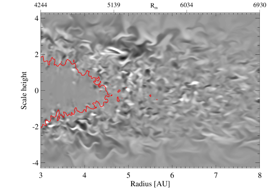
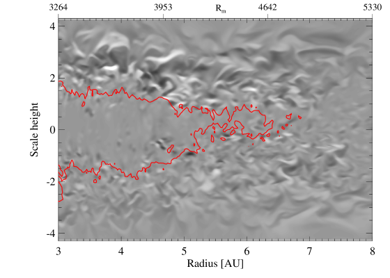
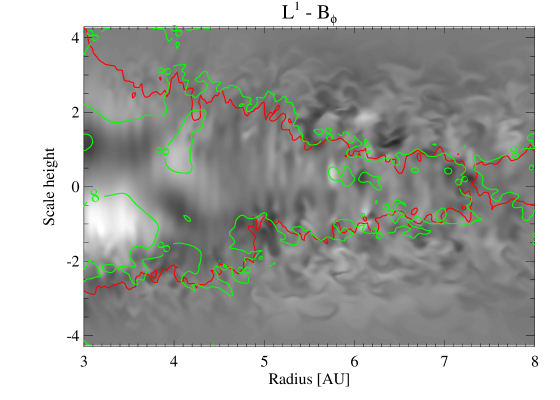
Fig. 4 presents a 2D slice of radial magnetic field overplotted with the line for model and after 1000 years.
At around the dissipation starts to damp the MRI at the midplane while there is still MRI turbulence in the corona of the disk. A similar shape could be expected at
the outer edge of dead-zones (Dzyurkevich et al. 2012, ApJ subm.).
We summarize that for magnetic Reynolds numbers above we observe a saturated and converged MRI turbulence in zero-net flux stratified simulations down to the midplane region.
The Maxwell stress dominates in each region the Reynolds stress.
Below the turbulence starts to decay at the midplane. The Elsasser number drops below 1 and there regions with low magnetic fields and dominating Reynolds stress.
At around , the Elsasser number drops below 0.1 at the midplane. Long-period oscillations becomes visible with MRI activation and decays. Below the MRI cannot operate. Here, Reynolds stress dominates over the Maxwell stress. Dependent on the surroundings, the upper layers are still active having MRI turbulence.
The results show that for magnetic Reynolds numbers down to , the MRI driven by a zero-net flux azimuthal magnetic field, can sustained the turbulence with .
Models and with show a decrease of the turbulence and eventually a dominating Reynolds stress.
From this results we conclude that the critical magnetic Reynolds number should around .
Oishi & Mac Low (2011) also found a critical magnetic Reynolds number around in local box simulations.
In the next chapter we concentrate on the run which present similar conditions as they are present in dead-zones.
3.3 Dead-zone oscillation
Before we move to the hydro-dynamical motions in dead-zones we want to investigate the long-term oscillations of the Maxwell stress we observed in the previous chapter. This oscillations could be connected to some sort of dynamo process.
Simon et al. (2011) presented in local box simulations a sudden transition from a ’low’ turbulent state to a ’high’ turbulent state. We observe in model and for a similar effect.
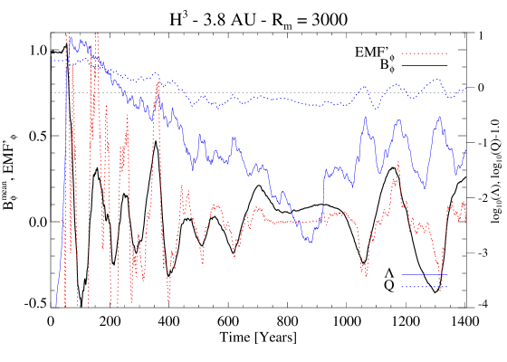
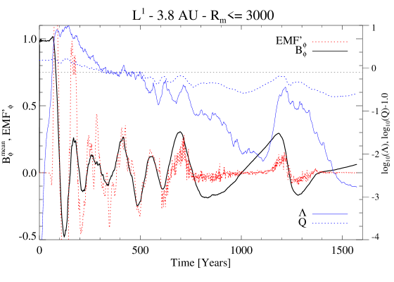
The results are combined in Fig 5 showing the mean toroidal magnetic field overplotted with the turbulent (times 1000), the Elsasser number and the Q value.
For this analysis we choose the southern hemisphere between 0 and 1.5 scale heights.
After around 200 years the initial mean toroidal magnetic field (black solid line) vanishes and starts to oscillate. There is a clear correlation between the turbulent EMF (red dotted line)
and the mean field which indicates a working dynamo. In both models, after around
500 years the MRI from azimuthal magnetic fields becomes unresolved ( blue dotted line below black dotted line). Here the Elsasser number drops below unity which still allows for damped MRI growth.
After 800 years the Elsasser number drops below 0.1. At this stage there is no MRI working and we are in the dead-zone stage. Here also the oscillations of mean field and turbulent EMF stop. In model the MRI switch on again after less then
200 years (27 local orbits) with a larger oscillation period. In model we observe a late switch on at 1100 years for only 150 years (20 local orbits). Afterwards the Elsasser number reaches nearly and we don’t expect a relaunch again. The sudden increase of is due to a sudden increase of poloidal magnetic field.
This sudden increase could be connected with the accumulation of toroidal magnetic fields (black solid line in Fig. 5, bottom) in the dead-zone
as well as due to radial transport of magnetic field (see chapter 3.5).
In Fig. 6, we present an azimuthal slice of toroidal magnetic field in the plane after 1500 years for model .
In the dead-zone () we observe locally a Q factor of 8 and above which correspond
to a plasma beta below 50, still the dissipation is too high to relaunch the MRI growth by azimuthal fields.
In general the line of resolved azimuthal field matches the one of decaying MRI (compare Fig. 3).
3.4 Hydrodynamical motions
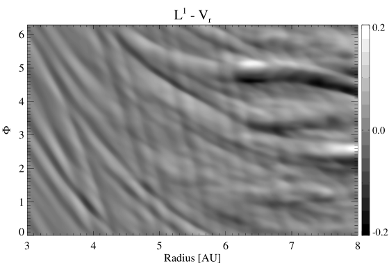
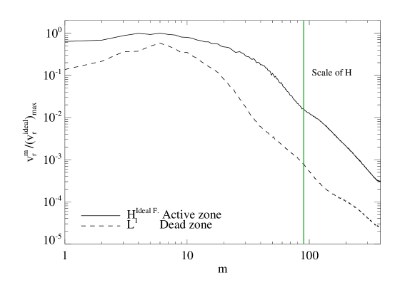
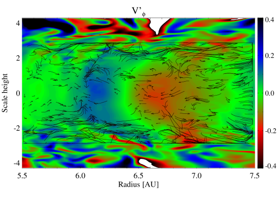
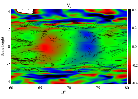
This dead-zone region is also interesting in terms of the hydro-dynamical motions. A close looks at the radial velocity in the midplane in Fig. 7 reveals velocity amplitudes around . On the first look these hydro-dynamical waves appear to be linear waves with a single mode. But a closer look at the Fourier spectra of the radial velocity reveals a more detailed picture. We calculated the spectra in the dead-zone region between 4 and 5 AU, time averaged between 1300 and 1500 years in model . In Fig. 8, we compare this spectra with the one obtained in fully ionized disk from model . In the dead-zone there is a peak at . The turbulence at lower scales (green solid line) is around 1 order of magnitude below the value in the fully MRI turbulent region. Beside the density waves we observe anti-cyclonic vortices (Fig. 7 between 6 and 7 AU) which create large extended spiral arms. They are produced at around 8 AU where we have a positive density slope due to the buffer zones. We calculated the relative vorticity between and in the large vortex. The growth of vortices at the border of the dead zone can be due to the Rossby wave instability as proposed by Varnière & Tagger (2006) and recently investigated by Lyra & Mac Low (2012). The vortex structure is presented in Fig. 9. The vertical extension is around SH, the radial extension is and the azimuthal one is around . The vortex is dragged by the hydro-dynamical surroundings which gives him the concave (Fig. 9 , top, dominant radial inward velocity), convex (Fig. 9, bottom, ) shape respectively. The magnetic fields (Fig. 9, bottom black vectors) are not present inside the vortex but in the surrounding layers. We measure a plasma beta of inside the vortex compared to in the surrounding region.
3.5 Radial mixing
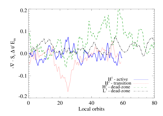
We already mentioned the effect of radial transport due to turbulent mixing. In this subsection we want to focus on the importance of radial transport of magnetic fields. We calculate the divergence of the radial Poynting flux integrated over time for the total and domain at using one scale height in radius. We integrate the divergence of the radial Poynting flux over every output ( local orbits) and compare it with the total magnetic energy. Fig. 10 shows how much magnetic energy is transported at each output (0.1 local orbits). In the fully turbulent layers the net radial transport is around zero with fluctuations of around 5 %. In the transition zone and the dead-zone the radial transport becomes more important and these fluctuations reach peaks of 10 to 20 %.
4 Discussion
4.1 Turbulence between active and dead-zones
In our work we showed that the MRI turbulence saturates around with .
Here the Elsasser number is around . This turbulence level is sustained for Elsasser number values of .
Stratified converged ideal MHD local simulations
(Davis et al., 2010) presented similar values of .
Still our results indicate a higher turbulence level using small explicit resistivity. High resolution simulations using explicit resistivity are needed to confirm the convergence of the accretion stress.
In addition, there are mean-field mechanism, which can temporal increase the value of
(Flock et al., 2012).
For magnetic Reynolds numbers around the critical value we observe long-period oscillations of the accretion stress as well as irregular switch off and on of MRI activity. Such oscillations were also reported by Simon et al. (2011) in local box simulations. We see indications that these oscillations are trigger by some dynamo process as locally there are accumulations of strong mean toroidal fields in the dead-zone. Also radial transport of magnetic field could here play a role.
In such configurations the corona is still active while in the midplane the MRI is switched of.
Here the Reynolds stress dominate over the Maxwell stress at .
A similar classification of turbulent regions in proto-planetary disks was done by comparing different heights,
see also in Okuzumi & Hirose (2011), Fig. 1.
4.2 Numerical, explicit and turbulent dissipation
In such turbulent simulations there are 3 kinds of important dissipation sources. The numerical dissipation, due to the finite grid size, the explicit resistivity and the turbulent dissipation. In model the numerical dissipation plays an important role. In addition one has to note that using a uniform grid, the numerical dissipation will be larger at the inner part then in the outer part. Here a logarithmic increasing grid would help. Then there is of course the explicit dissipation which is included in the induction equation in the code. Here one should be sure that the explicit one is higher than the numerical one. The turbulent dissipation scales with the level of the turbulence. Here it is still unclear how this dissipation process works in detail, see also Fig. 9 in Fromang & Papaloizou (2007).
5 Summary
We performed 3D global ideal and non-ideal MHD simulations to study MRI turbulence in low-ionized proto-planetary disks using an initial toroidal magnetic field for a range of magnetic Reynolds numbers. With our global simulations we are able to investigate the transition regime which is present between the active and the dead-zone in proto-planetary disks. We define 3 different disk regimes dependent on the magnetic Reynolds numbers:
-
•
Above a Reynolds number of . Here MRI turbulence saturates and is sustained. For this region we find steady and converged values around 0.01 in ideal and non-ideal simulations. The Maxwell stress dominates down to the midplane region. The turbulent velocities reach maximum values around . The dynamo is operating and we find with a positive sign in the northern hemisphere. The Elsasser number stays above 1 in the midplane.
-
•
Reynolds number between . Here, the MRI starts to switch of at the midplane region. The Elsasser number drops below 1. Simulations with show a still sustained turbulence, supported by radial transport of magnetic fields. For the MRI turbulence starts to switch off. We expect the critical magnetic Reynolds number around and below.
-
•
Reynolds number around and below. Here, there is no MRI at the midplane anymore. The Elsasser number drops below 0.1. The turbulence is dominated by the Reynolds stress. We observe long-period oscillations of MRI activity and MRI decay. There is an accumulation of toroidal magnetic fields below in the dead-zone. The turbulence at the midplane is supported by active channels in the corona which pump sound wave into the midplane region. The velocity spectra at the midplane reveals a drop of one order of magnitude at the scale of H in the dead-zone compared to the fully ionized turbulent region. We observe long lived anti-cyclonic vortices in the transition regime, creating spiral arms in the dead-zone. Magnetic fields are not present in the inner part of the vortex.
We thank Sebastien Fromang for the helpful comments on the global models. We thank Natalia Dzyurkevich for her suggestions and comments during this work. We thank also Neal Turner, Satoshi Okuzumi and Héloïse Meheut for their revision. We thank Andrea Mignone for supporting us with the PLUTO code. The research leading to these results has received funding from the European Research Council under the European Union’s Seventh Framework Programme (FP7/2007-2013) / ERC Grant agreement n° 258729. Parallel computations have been performed on the Theo cluster of the Max-Planck Institute for Astronomy Heidelberg located at the computing center of the Max-Planck Society in Garching.
References
- Bai (2011) Bai, X.-N. 2011, ApJ, 739, 50
- Balbus & Hawley (1991) Balbus, S. A. & Hawley, J. F. 1991, ApJ, 376, 214
- Balbus & Hawley (1998) —. 1998, Reviews of Modern Physics, 70, 1
- Beckwith et al. (2011) Beckwith, K., Armitage, P. J., & Simon, J. B. 2011, MNRAS, 416, 361
- Blaes & Balbus (1994) Blaes, O. M. & Balbus, S. A. 1994, ApJ, 421, 163
- Davis et al. (2010) Davis, S. W., Stone, J. M., & Pessah, M. E. 2010, ApJ, 713, 52
- Dzyurkevich et al. (2010) Dzyurkevich, N., Flock, M., Turner, N. J., Klahr, H., & Henning, T. 2010, A&A, 515, A70
- Fleming & Stone (2003) Fleming, T. & Stone, J. M. 2003, ApJ, 585, 908
- Fleming et al. (2000) Fleming, T. P., Stone, J. M., & Hawley, J. F. 2000, ApJ, 530, 464
- Flock et al. (2010) Flock, M., Dzyurkevich, N., Klahr, H., & Mignone, A. 2010, A&A, 516, A26
- Flock et al. (2012) Flock, M., Dzyurkevich, N., Klahr, H., Turner, N., & Henning, T. 2012, ApJ, 744, 144
- Flock et al. (2011) Flock, M., Dzyurkevich, N., Klahr, H., Turner, N. J., & Henning, T. 2011, ApJ, 735, 122
- Fromang & Nelson (2006) Fromang, S. & Nelson, R. P. 2006, A&A, 457, 343
- Fromang & Papaloizou (2007) Fromang, S. & Papaloizou, J. 2007, A&A, 476, 1113
- Gardiner & Stone (2005) Gardiner, T. A. & Stone, J. M. 2005, Journal of Computational Physics, 205, 509
- Hawley & Balbus (1991) Hawley, J. F. & Balbus, S. A. 1991, ApJ, 376, 223
- Inutsuka & Sano (2005) Inutsuka, S. & Sano, T. 2005, ApJ, 628, L155
- Jin (1996) Jin, L. 1996, ApJ, 457, 798
- Lyra & Mac Low (2012) Lyra, W. & Mac Low, M.-M. 2012, ArXiv e-prints
- Martin et al. (2012) Martin, R. G., Lubow, S. H., Livio, M., & Pringle, J. E. 2012, MNRAS, 2271
- Mignone et al. (2012) Mignone, A., Flock, M., Stute, M., Kolb, S. M., & Muscianisi, G. 2012, ArXiv e-prints
- Miyoshi & Kusano (2005) Miyoshi, T. & Kusano, K. 2005, Journal of Computational Physics, 208, 315
- Oishi & Mac Low (2009) Oishi, J. S. & Mac Low, M.-M. 2009, ApJ, 704, 1239
- Oishi & Mac Low (2011) —. 2011, ApJ, 740, 18
- Okuzumi & Hirose (2011) Okuzumi, S. & Hirose, S. 2011, ApJ, 742, 65
- Sano et al. (2000) Sano, T., Miyama, S. M., Umebayashi, T., & Nakano, T. 2000, ApJ, 543, 486
- Sano & Stone (2002a) Sano, T. & Stone, J. M. 2002a, ApJ, 570, 314
- Sano & Stone (2002b) —. 2002b, ApJ, 577, 534
- Simon et al. (2011) Simon, J. B., Hawley, J. F., & Beckwith, K. 2011, ApJ, 730, 94
- Turner et al. (2010) Turner, N. J., Carballido, A., & Sano, T. 2010, ApJ, 708, 188
- Turner & Sano (2008) Turner, N. J. & Sano, T. 2008, ApJ, 679, L131
- Turner et al. (2007) Turner, N. J., Sano, T., & Dziourkevitch, N. 2007, ApJ, 659, 729
- Varnière & Tagger (2006) Varnière, P. & Tagger, M. 2006, A&A, 446, L13