A PRQ Search Method for Probabilistic Objects

Abstract

This article proposes an PQR search method for probabilistic objects. The main idea of our method is to use a strategy called pre-approximation that can reduce the initial problem to a highly simplified version, implying that it makes the rest of steps easy to tackle. In particular, this strategy itself is pretty simple and easy to implement. Furthermore, motivated by the cost analysis, we further optimize our solution. The optimizations are mainly based on two insights: (i) the number of effective subdivisions is no more than 1; and (ii) an entity with the larger span is more likely to subdivide a single region. We demonstrate the effectiveness and efficiency of our proposed approaches through extensive experiments under various experimental settings.

I Introduction

Range query for moving objects has been the subject of much attentions [7, 10, 14, 22, 24], as it can find applications in various domains such as the digital battlefield, mobile workforce management, and transportation industry. It is usual that for a moving object $o$, only the discrete location information is stored on the database server, due to various reasons such as the limited battery power of mobile devices and the limited network bandwidth [4]. The recorded location of $o$ can be obtained by accessing the database, the whereabouts of its current location is usually uncertain [23]. For example, a common location update policy called dead reckoning [4, 23] is to update the recorded location ${l_{r}}$ when the deviation between ${l_{r}}$ and the actual location of $o$ is larger than a given distance threshold $\tau$. Before the next update, the specific location of $o$ is uncertain, except knowing that it lies in a circle with the center $l_{r}$ and radius $\tau$. To capture the location uncertainty, the idea of incorporating uncertainty into moving objects data has been proposed [23]. From then on, the probabilistic range query (PRQ) as a variant of the traditional range query has attracted much attentions in the data management community [5, 17, 15, 3, 20, 4, 25, 19]. A well known uncertainty model is using a closed region (in which the object can always be found) together with a probability density function (PDF). The closed region is usually called uncertainty region, and the PDF is used to denote object’s location distribution [4, 3, 23]. (See Section II for a more formal definition.) Given a query range $R$, the main difference between the traditional range query and the PRQ is that the latter returns not only the objects being located in $R$ but also their appearance probabilities. Assume that the location of object $o$ follows uniform distribution in its uncertainty region $u$ for ease of discussion, the probability of object $o$ being located in $R$ is equal to the ratio of the two areas, i.e., the probability $p=\frac{area~{}of~{}u\cap R}{area~{}of~{}u}$. Figure 1(a) illustrates an example and the PRQ returns { ($o$, 39%) }.

In existing works, an important branch is to address the PRQ for objects moving freely in 2D space. In this branch, many uncertainty models and techniques are proposed for various purposes. (Section II-A gives a brief survey about those models, purposes and techniques.) Surprisingly, little efforts are made for the PRQ over objects moving in a constrained 2D space where objects are forbidden to be located in some specific areas. For clarity, we term such specific areas as restricted areas, and dub the query above the Constrained Space Probabilistic Range Query (CSPRQ). The CSPRQ can also find many applications as objects moving in a constrained 2D space are common in the real world. For example, the tanks in the digital battlefield usually cannot run in lakes, forests and the like, the areas occupied by those obstacles can be naturally regarded as restricted areas (of tanks). With similar observations, in a zoo, tourists usually cannot roam in the dwelling spaces of dangerous animals such as tigers and lions, those dwelling spaces can be regarded as the restricted areas (of tourists).

Existing solutions cannot be directly applied to the CSPRQ as it involves a set ${\mathscr{R}}$ of restricted areas. Imagine if we directly use existing methods, implying that we ignore each restricted area $r$ ($\in{\mathscr{R}}$) in the computation phase. Figure 1(b) depicts this case, the circle $o.\odot$ is regarded as the uncertainty region $u$, and the query answer is {($o_{1}$, 100%), ($o_{3}$, 56%), ($o_{4}$, 42%)}. In contrast, Figure 1(c) presents the case considering ${\mathscr{R}}$ in the computation phase, here $o.\odot-\bigcup_{r\in R}r$ is regarded as $u$, and the query answer is { ($o_{1}$, 100%), ($o_{3}$, 22%), ($o_{4}$, 76%)}. The two answers above are different, and clearly the second one is correct. At first sight, to process the CSPRQ is simple as it seems to be a straightforward adaptation of existing methods. The fact however is not so, as this idea will be confronted with the overcomplicated geometrical operations, rendering its implementation infeasible. (Section III gives more detailed explanations.) In addition, computing the uncertainty region $u$ is also not a simple subtraction operation, as a straightforward computation incurs possible mistakes. On the other hand, the CSPRQ needs to consider a new set ${\mathscr{R}}$ compared to the previous works, it implies that the amount of data to be processed is larger and the computation is more complicated, which is another challenge and thus needs more considerations.

(a)

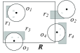
(b)

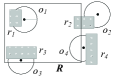
(c)

Figure 1: Illustration of the PRQ and CSPRQ. The small black dot denotes the recorded location $l_{r}$, the radius of circle denotes the distance threshold $\tau$, the biggest rectangle denotes query range $R$, the small rectangle denotes the restricted area $r$.

Motivated by the fact above, this paper makes the effort to the CSPRQ. The key idea of our solution is to use a strategy called pre-approximation that can reduce the initial problem to a highly simplified version, implying that it makes the rest of steps easy to tackle. In particular, this strategy itself is pretty simple and easy to implement. To operate different entities in a unified and efficient manner, a label based data structure is developed. Ascribing the pre-approximation and label based data structure, it is pretty simple to compute the appearance probability. To improve the I/O efficiency, a twin index is naturally adopted. Furthermore, motivated by the cost analysis, we further optimize our solution. The optimizations are mainly based on two insights: (i) the number of effective subdivisions is no more than 1, we utilize this insight to improve the power pruning restricted areas; and (ii) an entity with the larger span is more likely to subdivide a single region, this insight motivates us to sort the entities to be processed according to their spans. In addition to the main insights above, we also realize two other (simple but usually easy to ignore) facts and utilize them. Specifically, two mechanisms are developed: postpone processing and lazy update. After we finish the main tasks of this work, we also attempt another approach inspired by the curiosity, its basic idea is to precompute uncertainty regions and index them. Unfortunately, this approach suffers a non-trivial preprocessing time although it outperforms the aforementioned approaches in terms of both query and I/O performance. This extra finding offers us an important indication sign for the future research. In summary, we make the following contributions.

We formulate the CSPRQ based on an extended uncertainty model, and analyse its unique properties.

We show a straightforward solution will be confronted with non-trivial troubles, rendering its implementation infeasible. We also show it is (almost) infeasible to develop an exact solution.

We propose our solution that utilize an (extremely) important but pretty simple strategy.

We further optimize our solution based on two insights and two (simple but usually easy to ignore) facts.

We demonstrate the performance of our solution through extensive experiments under various experimental settings.

We report an extra finding that offers an important indication sign for the future research.

In the next section we formulate the problem to be studied and review the related work. We analyse this problem and propose our solution in Section III and IV, respectively. We further optimize our solution in Section V. We attempt the precomputation based approach in Section VI. We evaluate the efficiency and effectiveness of our proposed algorithms through extensive experiments in Section VII. Finally, Section VIII concludes this paper with several interesting research topics.

II Problem definition

Given a territory $\mathbb{T}$ with a set ${\mathscr{R}}$ of disjoint restricted areas, we assume there exist a set $\mathscr{O}$ of moving objects that can freely move in $\mathbb{T}$ but cannot be located in any restricted area $r$ ($\in{\mathscr{R}}$), and assume the last sampled location of each moving object $o$ is already stored on the database server. (Note that in this paper the terms the last sampled location and recorded location are used interchangeably.) Moreover, suppose each object $o$ reports its new location to the sever when the deviation between the recorded location $l_{r}$ and the actual location of $o$ is larger than a given distance threshold $\tau$. We denote the location of $o$ at an arbitrary instant of time $t$ by $l_{t}$. Furthermore, for any two different moving objects $o$ and $o^{\prime}$, we assume they cannot be located in the same location at the same instant of time $t$, i.e., $l_{t}\neq l_{t}^{\prime}$. Since the realistic application environment varies from place to place, the shapes of restricted areas should be diversified, whereas our objective is to establish a general approach instead of focusing on certain specific environment. Therefore throughout this paper we use polygons to denote the restricted areas (note: this assumption is feasible, since any shaped area can be transformed into polygon shaped area beforehand). Finally, we set the following conditions are always satisfied:

$$l_{t}\notin\bigcup_{r\in{\mathscr{R}}}{r}$$ (1a)

$$l_{t}\in{\mathbb{T}}-\bigcup_{r\in{\mathscr{R}}}{r}$$ (1b)

$$\bigcup_{r\in{\mathscr{R}}}{r}\subset{\mathbb{T}}$$ (1c)

The specific location of $o$ at the current time is usually uncertain, a well known model [4, 23] allows us to capture the location uncertainty of $o$ through two components:

Definition 1 (Uncertainty region).

The uncertainty region of a moving object $o$ at a given time $t$, denoted by $u^{t}$, is a closed region where $o$ can always be found.

Definition 2 (Uncertainty probability density function).

The uncertainty probability density function of a moving object $o$ at a given time $t$, denoted by $f^{t}(x,y)$, is the PDF of $o$’s location at the time $t$. Its value is $0$ if $l_{t}$ $\notin$ $u^{t}$.

Note that under the distance based update policy (a.k.a. dead-reckoning policy [4]), for any two different time $t_{1}$ and $t_{2}$, we have (i) $u^{t_{1}}=u^{t_{2}}$ and (ii) $f^{t_{1}}(x,y)=f^{t_{2}}(x,y)$, where $t_{1}$, $t_{2}\in$ ($t_{r}$, $t_{n}$], $t_{r}$ refers to the latest reporting time, and $t_{n}$ refers to the current time. In view of these, in the remainder of the paper we use $u$ and $f(x,y)$ to denote the uncertainty region and PDF of $o$, respectively. Since $f(x,y)$ is a PDF, in theory, it has the property:

$$\int_{{u}}f(x,y)dxdy=1$$ (2)

Under the distance based update policy, the uncertainty region $u$ can be derived based on the following formula [4, 23].

$$u={{C}}(l_{r},\tau)$$ (3)

where ${{C}}(\cdot)$ denotes a circle with the centre $l_{r}$ and radius $\tau$. For convenience, we use $o.\odot$ to denote this region. The above representation is feasible under the case no restricted areas exist, i.e., ${\mathscr{R}}=\emptyset$. Whereas the real uncertainty region $u$ for our problem should be as follows.

$$u=o.\odot-\bigcup_{r\in{\mathscr{R}}}r$$ (4)

Definition 3 (Constrained space probabilistic range query).

Given a set $\mathscr{R}$ of restricted areas and a set $\mathscr{O}$ of moving objects in a territory $\mathbb{T}$, and a query range $R$, the constrained space probabilistic range query returns a set $\mathscr{O}^{\prime}$ ($\subseteq\mathscr{O}$) of objects together with their appear probabilities in form of ($o$, $p$) such that for any $o\in\mathscr{O}^{\prime}$, $p\neq 0$, where $p$ is the probability of ${o}$ being located in ${R}$, and is computed as $p=\int_{u\cap R}f(x,y)dxdy$.

Note that in this paper we assume the distance based update policy is adopted. We abuse the notation ’$|\cdot|$’ but its meaning should be clear from the context. In addition, a notation or symbol with the subscript ’b’ usually refers to its corresponding MBR (e.g., $o.\odot_{b}$ refers to the MBR of $o.\odot$). For ease of reading, we summarize the frequently used symbols in Table I.

Symbols	Description
$R$	query range
$o$	moving object
$\mathscr{O}$	the set of moving objects
$r$	restricted area
$\zeta$	the number of edges of $r$
$\mathscr{R}$	the set of restricted areas
$\tau$	distance threshold
$l_{r}$	the recorded location of $o$
$f(x,y)$	PDF of $o$’s location
$p$	probability of $o$ being located in $R$
$u$	uncertainty region
$s$	the intersection result between $R$ and $u$
$u_{o}$	the outer ring of $u$
$\varphi$	the intersection result between $R$ and $u_{o}$
$u_{h}$	the hole of $u$
$\mathscr{H}$	the set of holes in $u$
$\mathscr{O}^{*}$	the set of candidate moving objects
$\mathscr{R}^{*}$	the set of candidate restricted areas
$e$	the approximated equilateral polygon from $o.\odot$
$\xi$	the number of edges of $e$
$d$	a subdivision
$d^{e}$	the effective subdivision

TABLE I: symbols and their meanings

II-A Related work

In terms of probabilistic range query over uncertain moving objects, researchers have made considerable efforts, and many outstanding techniques and models have been proposed. In this subsection, we review those works most related to ours.

The uncertainty model used in this paper is developed based on [23, 4]. In their papers, a moving object $o$ updates its recorded location $l_{r}$, when the deviation (between its actual location and $l_{r}$) is larger than a given distance threshold $\tau$. This update policy is just the so-called distance based update policy. In particular, they discussed two types of moving objects: (i) moving on predefined routes, and (ii) moving freely in 2D space. For the former, the route consists of a series of line segments, the uncertainty is a line segment on the route, called line segment uncertainty (LSU) model for convenience. For the latter, the route is unneeded, and the uncertainty used in their paper is a circle, called free moving uncertainty (FMU) model. Our model roughly follows the latter. The difference is that our model introduces the restricted areas, and the uncertainty region $u$ is not necessarily a circle. (Although only a slight difference viewed from the surface, the amount of data to be processed in our query however is larger, and the computation is more complicated. In particular, a straightforward adaptation of their method will incur overcomplicated geometrical operations, rendering its implementation infeasible.)

In addition, the models in [18, 3] are the same or similar as the FMU model, and also focus on the case of no restricted areas. For example, Tao et al. [18] investigated range query on multidimensional uncertain data, they proposed a classical technique PCR, and an elegant indexing mechanism U-tree. They adopted a circle to represent the uncertainty region $u$ (see Section 7 in [18]). Chen et al. [3] addressed location based range query. Several clever ideas such as query expansion and query duality were proposed. They discussed two types of target objects: static and moving. They assume the uncertainty region $u$ is a rectangle when the target object is moving. (Note: our work does not belong to location based query. Location based CSPRQ should be more interesting, as the location of query issuer is also uncertain.)

Regarding to the case of objects moving freely in 2D space, there are many other classical uncertainty models like, the MOST model [17], the UMO model [25], the 3D cylindrical (3DC) model [20, 15], and the necklace uncertainty (NU) model [19, 11]. These models have different assumptions and purposes, but also their own advantages (note: it is a difficult task to say which one is the best). The models in [17, 25] are developed for querying the future location. For example, Sistla et al. [17] proposed the MOST model, they assume the direction and speed of each object $o$ are available, and these information should be updated if the change occurs. The future location is predicted based on three parameters: velocity, direction, and time. Later, Zhang et al. [25] proposed the UMO model, in which they use the distribution of location and the one of velocity, instead of the exact values, to characterize the location uncertainty, and assume these distributions are available at the update time. The models in [20, 19, 15, 11] are suitable for querying the trajectories of moving objects. For example, Trajcevski et al. [20] proposed to model an uncertain trajectory as a 3D cylindrical body, they assume an electrical map, all recorded locations and sampling time are available. Later, they proposed the NU model [19], which can be viewed as an enhanced version of the 3DC model. In this model, they represent the whereabouts in-between two known locations as a bead, and an uncertain trajectory as a necklace (a sequence of beads). Our work is different from aforementioned works in at least two points: (i) those works focus on the case of no restricted areas, and (ii) the underlying uncertainty model is different from theirs. (Note: it should be more interesting to extend the concept of restricted areas to those uncertainty models.)

Recently, Emrich et al. [6] proposed to model the trajectories of moving objects by stochastic processes, they assume the object is in a discrete state space (i.e., a finite set of possible locations in space), and assume the transition probability (from a state to another state) is available. Our work is different form theirs in two points at least: (i) the underlying models are different, and (ii) the object discussed in our paper is not in a discrete state space.

Another important branch is to focus on objects moving on predefined routes (or road networks) [5, 26]. For example, Chung et al. [5] adopted the LSU model to process range query, and proposed a clever idea — transforming the uncertain movements of objects into points in a dual space using the Hough Transform. To query the trajectories of objects moving on road networks, Zheng et al. [26] proposed the uncertain trajectory (UT) model and an elegant indexing mechanism UTH. They assume all recorded locations and sampling time are available, and objects follow the shortest paths and travel at a constant speed between two consecutive trajectory samples. Our work is different from works mentioned above, as here we focus on objects moving in a constrained 2D space where no predefined routes are given.

III Problem analysis

At first sight, to process the CSPRQ is simple as it seems to be a straightforward adaptation of existing methods. To process the PRQ, existing methods (see e.g., [4]) consist of three main steps.

For each object $o$, it computes $u\cap R$ if the uncertainty region $u$ intersects with the query range $R$.

It computes the probability $p$ based on a formula $p=\int_{u\cap R}f(x,y)dxdy$, and put the tuple ($o$, $p$) into the result.

It returns the result (which usually includes a series of tuples) after all objects are processed. By the large, we only need to add one step, i.e., computing the uncertainty region $u$ based on Equation 4 before checking if $u$ intersects with $R$. In other words, this straightforward method mainly consists of four steps. Now the readers should be pretty curious — why the four steps above cannot be (easily) achieved. We next look a bit deeper into those steps above, and then we can easily realize four main issues (but not limited to) arise.

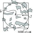
(a)

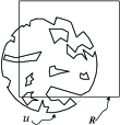
(b)

(c)

Figure 2: Illustration of a straightforward solution. (a) The grey polygon illustrates the restricted area $r$, the circle illustrates $C(l_{r},~{}\tau)$, i.e., $o.\odot$. (b) The biggest rectangle illustrates the query range $R$, the pseudo circle illustrates the uncertainty region $u$. (c) It is the intersection result of $u\cap R$.

First, suppose the location of an object $o$ follows uniform distribution in its uncertainty region $u$, the following equation holds [15]:

$$p=\frac{\Lambda(u\cap R)}{\Lambda(u)}$$ (5)

where $\Lambda(\cdot)$ denotes the area of the geometrical entity. Let $s$ be the intersection result of $u\cap R$. It is easy to know that computing the area of $u$ (or $s$) is simple for the case of no restricted areas. To the case of our concern, e.g., see Figure 2, how to compute the area of $u$ (or $s$)? Computing the area of such complicated entity is not an easy task, as its boundary consists of both straight line segments and curves, and it includes many holes. (In fact, $s$ possibly consists of multiple subdivisions in addition to holes. Those even more complicated cases will be discussed in Section V.) A natural method could be to divide the entity into multiple small strips shown in Figure 3(a), and then to compute the area of each strip and add them together. In practice, this solution however, is overcomplicated and difficult to implement.

(a)

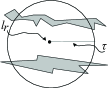
(b)

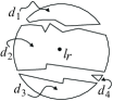
(c)

Figure 3: Illustration of computing the area and uncertainty region $u$. The grey polygon illustrates the restricted area $r$, the circle illustrates $C(l_{r},~{}\tau)$, i.e., $o.\odot$.

Second, suppose the location of $o$ does not follow uniform distribution in $u$, a usually used method is the Monte Carlo method. Its basic idea is to randomly generate $N_{1}$ points in $u$. For each generated point $p^{\prime}$, it computes $f(x_{i},y_{i})$, where ($x_{i},~{}y_{i}$) is the coordinates of the point $p^{\prime}$, and then checks whether or not $p^{\prime}\in s$. Without loss of generality, suppose $N_{2}$ points (among $N_{1}$ points) are to be located in $s$. Finally, it gets the probability $p$ as follows.

$$p=\frac{\sum_{i=1}^{N_{2}}{f{(x_{i},~{}y_{i})}}}{\sum_{i=1}^{N_{1}}{f{(x_{i},~{}y_{i})}}}$$ (6)

Given a randomly generated point $p^{\prime}$, to check whether or not $p^{\prime}\in u$ (or $p^{\prime}\in s$) is simple if no restricted areas exist. However, it is not an easy task for the case of our concern. Note that the solutions to the point in polygon problem [9, 1] cannot be applied to our context as geometrical entities considered here are more complicated.

Third, it is easy to know that both $u$ and $s$ are pretty simple if no restricted areas exist. Geometrical entities in our context however are more complicated. Then, how to represent and operate them in a concise and efficient way?

Fourth, computing $u$ is not a straightforward subtraction operation. Figure 3(b) illustrates the case before executing the subtraction operation, and the subtraction result is shown in Figure 3(c), which has four subdivisions. Note that, only $d_{2}$ is the real uncertainty region, other subdivisions are invalid, the reason will be explained in the next section.

Besides the issues mentioned above, we should note that the amount of data to be processed is larger compared to the case of no restricted areas. It is easy to know that the PRQ only needs to check $O(|\mathscr{O}|)$ objects. In contrast, the CSPRQ needs to check $O(|\mathscr{R}|)$ restricted areas for each object $o$, the (worst case) complexity is $O(|\mathscr{R}||\mathscr{O}|)$.

Discussion. The above analysis offers insights into our problem, it reveals to us that to process the CSPRQ using a straightforward solution is infeasible. Furthermore, even if the location of $o$ follows uniform distribution in $u$, it is still non-trivial to develop an exact solution (let alone the non-uniform distribution case), implying that to develop an exact solution is also (almost) infeasible. After we realize the facts above, we also note that another easily brought to mind method that is to approximate the curves on the boundary of $u$ (or $s$) into line segments. In this way, the troubles shown before seemingly can be tackled easily. In fact, existing curve interpolation techniques can indeed transform the boundary of $u$ (or $s$) into line segments. It however is still inconvenient and inefficient, since there are too many such entities in the query processing. In addition, it is also difficult and troublesome to approximate curves into line segments in such a manner, as the shapes of different entities vary from one to another.

IV Our solution

The key idea of our solution is to use a strategy called pre-approximation that can lead to a highly simplified version of the initial problem, implying that it can make the rest of steps easy to tackle. In particular, this strategy itself is pretty simple and easy to implement.

IV-A Pre-approximation

The essence of the pre-approximation is that, it first transforms (or approximates) $o.\odot$ into an equilateral polygon denoted by $e$, and then uses $e$ to subtract the restricted areas. Thus, according to Equation 4, we have

$$u\doteq e-\bigcup_{r\in\mathscr{R}}r$$ (7)

To get $e$ is pretty simple, without loss of generality, assume that we need to approximate $o.\odot$ into an equilateral polygon $e$ with a number $\xi$ of edges. We actually only need to obtain each vertex of $e$, which can be computed based on the following equations.

$${x}_{i}=l_{r}.{x}+\tau\cdot\cos\frac{(i-1)\cdot{2\pi}}{\xi}$$ (8a)

$${y}_{i}=l_{r}.{y}+{\tau}\cdot\sin\frac{(i-1)\cdot{2\pi}}{\xi}$$ (8b)

where $i$$\in$$[1,2,\dots,{\xi}]$, ($l_{r}.x$, $l_{r}.y$) denote the coordinates of the recorded location $l_{r}$, and $({x}_{i},{y}_{i})$ denote the coordinates of the $i$th vertex of $e$.

Clearly, the larger (the) $\xi$ is, the more accurate results we can get. (In fact, our experimental results show the accuracy is pretty good even if we only set $\xi=32$.) Note that, here ${o}.\odot$ is the circumscribed circle of $e$, which can assure that the distance from any point in $e$ to the center is always less than the distance threshold $\tau$. The main reasons we do this transformation are as follows: (i) it is convenient for the follow-up calculations since operating on line segments, in most cases, is more simple and efficient than on curves; (ii) it is easy to represent the calculated result; and (iii) all the troubles discussed in Section III can be significantly simplified. In the next section, we show how to represent different entities in a unified and efficient manner.

IV-B LBDS

Once the pre-approximation idea is adopted, the boundaries of all the geometrical entities will be no curves. Moreover, we observe that $u$ may be a closed region with hole(s) or just be a simple closed region, and $s$ possibly consists of multiple subdivisions with hole(s). For ease of operating these entities in a unified and efficient manner, we need a targeted data structure to represent them. (We remark that the doubly connected edge list (DCEL) [1] consists of three collections of records: one for the vertices, one for the faces, and one for the half-edges; to our problem, it is a little clunky and not intuitive enough.) We next introduce some basic definitions in order to easily describe the details of our proposal.

Definition 4 (Outer ring and inner ring).

Given a closed region $c$ with a hole $h$ , the boundary of $c$ and the one of $h$ are termed as the outer ring and inner ring of $c$, respectively.

Note that, if a closed region contains $n$ holes, it clearly has $n$ inner rings, see e.g., Figure 2(c). Specifically, in order to easily handle those entities, we present a label based data structure (LBDS), which consists of three domains — one label domain and two pointer domains.

Flag: This domain is the boolean type. Specifically, $0$ indicates the entity has no hole, and 1 indicates it has no less than one hole.

OPointer: This domain points to a simple polygon that denotes the outer ring of the entity. A simple polygon consists of two domains.

VPointer: This domain points to a linked list that stores a series of vertexes.

B: This domain stores the MBR of the polygon.

IPointer: This domain points to a linked list that stores the simple polygons, which denote the inner rings of this entity.

Hence $u$ can be represented by the LBDS directly, and $s$ can be represented by a linked list in which a series of ’LBDSs’ are stored. This structure is intuitive, concise, and convenient for the follow-up computation, its benefits will be demonstrated gradually in the rest of the paper.

IV-C Picking out the real uncertainty region

To compute the uncertainty region $u$ (by Formula 7) is straightforward, we can use the equilateral polygon $e$ to subtract each restricted area $r$ one by one. In Section III, we show that computing $u$ is not a simple subtraction operation. In other words, Formula 4 and 7 actually imply some possible mistakes, we slightly abuse them for presentation simplicity. In Figure 3(c), we say $d_{2}$ (rather than other three subdivisions) is the real uncertainty region, which is based on the lemma below.

Lemma 1 (Choose real uncertainty region).

Given $o.\odot$, $l_{r}$, $\tau$ and $\mathscr{R}$, we let $d$ be one of subdivisions after we execute the subtraction operation based on Equation 4. If $l_{r}\in d$, then $\surd$($d$), where $\surd$($\cdot$) denotes it is the real uncertainty region. Otherwise, $\lnot$($\surd$($d$)).

Proof. We first prove $l_{r}\notin d$ $\Rightarrow$ $\lnot$($\surd$($d$)). According to Definition 1, we only need to show $o$ cannot be found in $d$. Clearly, $o$ must be located in $o.\odot$, since $l_{r}$ is the latest recorded location, and $\tau$ is the distance threshold. Furthermore, based on analytic geometry, it is easy to know that $o$ cannot reach $d$ if it does not walk out of $o.\odot$ (e.g., see Figure 3(b), $o$ cannot reach the topmost (or bottommost) region of $o.\odot$). Hence we cannot find $o$ in $d$.

The proof for the argument “$l_{r}\in d$ $\Rightarrow$ $\surd$($d$)” can be obtained using the similar method above; omitted due to space limit. $\square$

We remark that once the pre-approximation idea is used, to check whether or not $l_{r}\in d$ is simple, as it is just the point in polygon problem [9, 1]. After we obtain the real uncertainty region $u$, we can get $s$ by executing an intersection operation on $u$ and $R$. There are many algorithms (e.g., see [21, 8, 16, 12, 13]) that can perform intersection operation on polygons with holes. They however do not well consider the case of many holes. Even so, there is a simple method that is adapted from the algorithms mentioned above. Its general idea is to compute the intersection result between $R$ and the outer ring of $u$ at first, and then to use this intersection result to subtract each inner ring of $u$ one by one, finally it gets $s$.

IV-D The appearance probability

For uniform distribution PDF, the crucial task is to compute the areas of $u$ and $s$ (cf. Equation 5). We show in Section III that computing these areas using a straightforward solution is overcomplicated. Now, we can easily compute them using the following method, which ascribes the pre-approximation and LBDS. Let $u_{o}$ be the outer ring of $u$, and $u_{h}^{i}$ be the $i$th hole in $u$. Let $s[i]$ be the $i$th subdivision of $s$, $s[i]_{o}$ be the outer ring of $s[i]$, and $s[i]_{h}^{k}$ be the $k$th hole of $s[i]$. First, given a polygon denoted by $P$, its area can be easily obtained based on the following equation [2].

$$\Lambda(P)=\frac{1}{2}\cdot\left(\left|\begin{array}[]{cc}x_{1}&x_{2}\\ y_{1}&y_{2}\end{array}\right|+\left|\begin{array}[]{cc}x_{2}&x_{3}\\ y_{2}&y_{3}\end{array}\right|+...+\left|\begin{array}[]{cc}x_{n}&x_{1}\\ y_{n}&y_{1}\end{array}\right|\right)$$ (9)

where $\left|\begin{array}[]{cc}x_{1}&x_{2}\\ y_{1}&y_{2}\end{array}\right|$$=(x_{1}\cdot y_{2}-x_{2}\cdot y_{1})$, and $(x_{1},y_{1})$ denote the coordinates of a vertex, other symbols have similar meanings. Furthermore, since we use the LBDS to represent $u$, and polygons are the basic elements of the LBDS, the area of $u$ can be obtained as follows.

$$\Lambda(u)=\Lambda(u_{o})-\sum_{i=0}^{|\mathscr{H}|}\Lambda(u_{h}^{i})$$ (10)

where $|\mathscr{H}|$ ($\geq 0$) is the number of holes in $u$. Similarly, since $s$ consists of a series of LBDSs, we have

$$\Lambda(s)=\sum_{i=1}^{|s|}\Lambda(s[i])=\sum_{i=1}^{|s|}{(\Lambda(s[i]_{o})-\sum_{k=0}^{|s[i]_{h}|}\Lambda(s[i]_{h}^{k})}$$ (11)

where $|s|$ ($\geq 1$) is the number of subdivisions of $s$, $|s[i]_{h}|$ ($\geq 0$) is the number of holes in $s[i]$. For arbitrary distribution PDF, we also use the Monte Carlo method to compute the probability $p$. We should note that the trouble shown in Section III does not exist now, as no curve is on the boundary of $u$ (or $s$), ascribing the pre-approximation idea.

IV-E Query processing

A naive method is to do a linear scan — for each object $o$, it scans each restricted area $r$, and compute $u$ based on Formula 7, and then compute the probability $p$ if $u$ intersects with $R$. Clearly, it is inefficient to process the CSPRQ in such a way. We now present another natural but more efficient method as follows. Let $R_{b}$, $r_{b}$ and $o.\odot_{b}$ be the MBRs of $R$, $r$ and $o.\odot$, respectively.

Definition 5 (Candidate moving object).

Given the query range $R$ and a moving object $o$, $o$ is a candidate moving object such that $R_{b}\cap$$o.\odot_{b}$$\neq$$\emptyset$.

Definition 6 (Candidate restricted area).

Given a restricted area $r$ and a moving object $o$, $r$ is a candidate restricted area such that $r_{b}\cap$$o.\odot_{b}$$\neq$$\emptyset$.

Let $\mathscr{O}^{*}$ be the set of candidate moving objects, and $\mathscr{R}^{*}$ be the set of candidate restricted areas of the object $o$. We can rewrite Formula 7 as follows.

$$u\doteq e-\bigcup_{r\in\mathscr{R}^{*}}r$$ (12)

The MBRs of the set $\mathscr{R}$ of restricted areas can be obtained easily, since each restricted area $r$ is static. Furthermore, since the recorded location $l_{r}$ and the distance threshold $\tau$ are already stored on the database server, the MBR of each moving object can be computed easily, it is a square centering at $l_{r}$ and with 2$\tau$ $\times$ 2$\tau$ size (in fact it is just the MBR of $o.\odot$). Clearly, for all restricted areas and moving objects, we can use a twin-index to manage their MBRs. For instance, we can build two R-trees (or a variant such as the R^∗- tree) to manage the MBRs of moving objects and the ones of restricted areas, respectively. Let $\mathscr{I}_{o}$ and $\mathscr{I}_{r}$ be the index of moving objects and the one of restricted areas, respectively. Our query processing algorithm is illustrated below.

 

Algorithm 1 Constrained space probabilistic range query  

(1)    Let $\Re=\emptyset$

(2)    Search $\mathscr{O}^{*}$ on $\mathscr{I}_{o}$ using $R_{b}$ as the input

(3)    for each $o\in\mathscr{O}^{*}$ do

(4)        Search $\mathscr{R}^{*}$ on $\mathscr{I}_{r}$ using $o.\odot_{b}$ as the input

(5)        Obtain $e$ based on Equation 8a and 8b

(6)        Compute $u$ based on Formula 12

(7)        if $u$ consists of multiple subdivisions then

(8)            Choose the real $u$ based on Lemma 1

(9)        Let $s=u\cap R$, and $p=0$

(10)       if $s\neq\emptyset$ then

(11)           if uniform distribution PDF then

(12)               Compute $p$ based on Equation 5, 9, 10 and 11

(13)           else // non-uniform distribution PDF

(14)               Compute $p$ based on Equation 6

(15)       if $p\neq 0$ then

(16)           Let $\Re=\Re\bigcup(o,p)$

(17)   return $\Re$  

Cost analysis. Let $C_{o}$ be the cost to search the set $\mathscr{O}^{*}$ of candidate moving objects. Clearly, we have

$$C_{o}\propto(|R_{b}|,~{}|\mathscr{O}|)$$ (13)

where $\propto$ means “is proportional to”, $|R_{b}|$ is the size of MBR of $R$, $|\mathscr{O}|$ is the cardinality of $\mathscr{O}$. Let $C_{r}$ be the cost to search the set $\mathscr{R}^{*}$ of candidate restricted areas. Similarly, we have

$$C_{r}\propto(|o.\odot_{b}|,~{}|\mathscr{R}|)$$ (14a)

$$|o.\odot_{b}|\propto\tau$$ (14b)

where $|o.\odot_{b}|$ is the size of MBR of $o.\odot$, $|\mathscr{R}|$ is the cardinality of $\mathscr{R}$, $\tau$ is the distance threshold of $o$. Let $C_{e}$ be the cost to obtain the equilateral polygon $e$. We have

$$C_{e}\propto\xi$$ (15)

where $\xi$ is the number of edges of $e$. Let $C_{u}$ be the cost to compute $u$ (line 6-8), and $\zeta$ be the average number of edges of restricted areas. We have

$$C_{u}\propto(\xi,~{}\zeta,~{}|\mathscr{R}^{*}|)$$ (16a)

$$|\mathscr{R}^{*}|\propto(\tau,~{}|\mathscr{R}|)$$ (16b)

where $|\mathscr{R}^{*}|$ is the cardinality of $\mathscr{R}^{*}$. Let $C_{s}$ be the cost to compute $s$, and $\gamma$ be the number of edges of $u_{o}$ (the outer ring of $u$). Since the set $\mathscr{R}^{*}$ of candidate restricted areas form the holes of $u$, the number of edges of hole is also $\zeta$. We have

$$C_{s}\propto(\gamma,~{}|u_{h}|,~{}\zeta)$$ (17a)

$$|u_{h}|\propto(\tau,~{}|\mathscr{R}^{*}|)$$ (17b)

Let $C_{p}^{u}$ be the cost to compute $p$ in the case of uniform distribution, and $C_{p}^{n}$ be the cost to compute $p$ in the case of non-uniform distribution. Note that each cost (in the for loop) refers to the average cost, and we overlook the cost of adding a tuple $(o,p)$ into $\Re$ as it is trivial. We also note that $C_{o}$ is related to $\mathscr{I}_{o}$ (e.g., the fan-out of $\mathscr{I}_{o}$), and $C_{r}$ is related to $\mathscr{I}_{r}$ (e.g., the fan-out of $\mathscr{I}_{r}$). We assume existing indexing technique is to be adopted, we hence omit this discussion in our analysis for simplicity. Let $C_{t}$ denote the total cost, we have

$$C_{t}= C_{o}+|\mathscr{O}^{*}|({C_{r}}+C_{e}+C_{u}+C_{s}+C_{p}^{u})$$ (18a)

$$C_{t}= C_{o}+|\mathscr{O}^{*}|({C_{r}}+C_{e}+C_{u}+C_{s}+C_{p}^{n})$$ (18b)

Clearly, to reduce the total cost $C_{t}$, we should reduce at least one sub-cost. Since $|\mathscr{O}|$ and $|\mathscr{R}|$ are depended on the application scenario, and $|R_{b}|$ is depended on the input of the user, we can easily know by Formula 13, 14a and 14b that there is little space to reduce $C_{o}$ and $C_{r}$. Furthermore, there is also (almost) no space to reduce $C_{e}$, as $\xi$ is used to assure the accuracy of our algorithm, and the natural solution to execute Equation 8a and 8b is already pretty efficient. We also note that our solution to compute the area of $u$ (or $s$) is already pretty simple and efficient, implying that there is also (almost) no space to reduce $C_{p}^{u}$. Regarding to $C_{p}^{n}$, it is mainly depended on the number $N_{1}$ of random generated points (cf. Equation 6), and $N_{1}$ is used to assure the accuracy of our algorithm. Naturally, we need to set $N_{1}$ to an acceptable value at least which can assure an allowable workload error. This implies that there is also no much space to reduce $C_{p}^{n}$. Recall Section IV-C, we compute $u$ and $s$ using the simple methods, which are somewhat inefficient, and for each single query, the cost to compute $u$ and $s$ is $|\mathscr{O}^{*}|(C_{u}+C_{s})$, which is non-trivial compared to $C_{t}$. (Note that in the previous works, $C_{u}=0$, $C_{s}$ is pretty small and almost can be overlooked, as $u$ is a circle in the case of no restricted areas.) These facts motivate us to further optimize our solution by reducing $C_{u}$ and $C_{s}$. In the next section, we show how to reduce $C_{u}$ and $C_{s}$ based on two insights and two simple but usually easy to ignore facts.

V Further optimize our solution

The optimizations are mainly based on two insights: (i) the number of effective subdivisions is no more than 1; and (ii) an entity with the larger span is more likely to subdivide a single region. In addition to the main insights above, we also realize two other (simple but usually easy to ignore) facts and utilize them; specifically, two mechanisms are developed: postpone processing and lazy update.

V-A Effective subdivision

Definition 7 (Effective subdivision).

Given $o.\odot$ and a set $\mathscr{R}^{*}$ of candidate restricted areas, without loss of generality, assume that $|{o.\odot}-r|>1$ when the $i$th “subtraction operation” is executed, where $|\cdot|$ denotes the number of subdivisions of the subtraction result, and $1\leq i\leq|\mathscr{R}^{*}|$. A subdivision $d$ is an effective subdivision such that the recorded location $l_{r}\in d$.

Lemma 2 (Number of effective subdivisions).

Assume that $|o.\odot-r|>1$, the number of effect subdivisions is no more than 1.

Proof. It follows from Definition 7 and analyst geometric, the details are omitted due to space limit. $\square$

Let $d^{e}$ be the effective subdivision when the $i$th “subtraction operation” is executed, where $1\leq i\leq|\mathscr{R}^{*}|$. We have

Lemma 3 (Subdivisions pruning).

Assume that $|o.\odot-r|>1$, all subdivisions except $d^{e}$ can be pruned safely.

Proof. By Lemma 2, we only need to show the uncertainty region $u\subseteq d^{e}$. This can be proved based on Lemma 1 and analyst geometric; omitted due to space limit. $\square$

Let $d_{b}^{e}$ be the MBR of the effective subdivision $d^{e}$. Lemma 2 and 3 indicate that we can immediately discard unrelated subdivisions once multiple subdivisions appear. In particular, we can use $d_{b}^{e}$ to prune the rest of candidate restricted areas, as it has a stronger pruning power compared to $o.\odot_{b}$. We remark that the entity $o.\odot$ is continuous evolving when it subtracts candidate restricted areas one by one, and in fact we use $e$ (rather than $o.\odot$) to do “subtraction operation”, as we adopt the pre-approximation strategy. We abuse the notation $o.\odot$ in Definition 7 and Lemma 2 and 3.

Comparison. The approach above is superior to the approach in Section IV-C (called the prior approach) in the following points (note that the prior approach chooses the real uncertainty region at the last step):

1. The prior approach needs to use each subdivision to subtract the rest of candidate restricted areas. In contrast, the approach above only needs to use $d^{e}$ to subtract the rest of candidate restricted areas. For instance, in Figure 4(b), the prior approach uses not only $d_{1}$ but also $d_{2}$ to subtract the rest of candidate restricted areas ($r_{2}$, $\cdots$, $r_{7}$), whereas the approach above only needs to use $d_{1}$ to subtract the rest of candidate restricted areas.

2. The prior approach cannot prune the rest of candidate restricted areas. In contrast, the approach above can prune the unrelated candidate restricted areas. For example, in Figure 4(b), the prior approach cannot prune candidate restricted areas as they are related to either $d_{1}$ or $d_{2}$, whereas the approach above can use the MBR of $d_{1}$ to prune $r_{2}$ and $r_{6}$, and use $d_{1}$ to prune $r_{7}$.

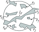
(a)

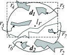
(b)

Figure 4: Illustration of subdivisions pruning and span. The grey polygons illustrate the set $\mathscr{R}^{*}$ of candidate restricted areas, and the big equilateral polygon illustrates $e$ with 32 edges.

We show the superiority of the approach above. The natural method to compute $u$ however, is using $e$ to randomly subtract each $r$ ($\in\mathscr{R}^{*}$) one by one (cf. Section IV-C), implying that $r_{1}$ in Figure 4 may be handled at last. In this case, the superiority of the approach above disappears. In the next section, we show how to maximize its superiority by utilizing the span.

V-B Span

Let $g$ be a 2D entity, and $g_{b}$ be the MBR of $g$. Let $(g_{b}.x^{-},~{}g_{b}.y^{-})$ and $(g_{b}.x^{+},~{}g_{b}.y^{+})$ be the left-bottom point and right-top point of $g_{b}$, respectively. We denote by $g_{s}$ the span of $g$, which is defined as follows.

Definition 8 (Span).

Given a 2D entity $g$, its span $g_{s}$ is computed as

$$g_{s}= g_{b}.x^{+}-g_{b}.x^{-}, g_{b}.x^{+}-g_{b}.x^{-} \geq g_{b}.y^{+}-g_{b}.y^{-}$$ if

$$g_{s}= g_{b}.y^{+}-g_{b}.y^{-},$$ otherwise

Heuristic 1.

A 2D entity with the larger span usually is more likely to subdivide a single (closed) region.

See Figure 4(a) for example. Clearly, here $e$ can be regarded as a single (closed) region, and each $r\in\mathscr{R}^{*}$ can be regarded as a 2D entity. Compared to other candidate restricted areas, here $r_{1}$ has the largest span and it is more likely to subdivide $e$ into multiple subdivisions. Heuristic 1 motivates us to handle $r$ that has the larger span as early as possible. This can be achieved by sorting their spans according to the descending order. We remark that the span is a real number, hence the overhead to sort $|\mathscr{R}^{*}|$ candidate restricted areas is pretty small, and (almost) can be overlooked compared to the overhead to execute $O(|\mathscr{R}^{*}|)$ times geometrical subtraction operations.

Another application. To compute $s$, the method in Section IV-C (called the prior method) uses the intersection result, denoted by $\varphi$ , between $u_{o}$ and $R$ to subtract each hole $u_{h}$. (Here $u_{o}$ refers to the outer ring of $u$.) We now show how to use the span of hole to improve the prior method. Let $\mathscr{H}$ be the set of holes of $u$.

Lemma 4 (Subdivisions retaining).

Given $\varphi$ and $u_{h}$, if $|\varphi-u_{h}|>1$, any subdivision of this subtraction result cannot be discarded, where $|\cdot|$ denotes the number of subdivisions.

proof. By contradiction, assume the subdivision $d$ ($\in\varphi-u_{h}$) can be discarded. This implies any point $p^{\prime}\in d$ can be discarded, i.e., $o$ cannot reach $p^{\prime}$ (from $l_{r}$) if it does not walk out of $o.\odot$. (Note that $d$ possibly contains or intersects with other holes, but the case $d$ itself being a hole is impossible. Otherwise, $d$ and $u_{h}$ form a larger hole as they are connected.) However, by the definition of $u$, $o$ can reach any point $p^{\prime}\in u_{o}-\bigcup_{u_{h}\in\mathscr{H}}u_{h}$ without the need of walking out of $o.\odot$, it is contrary to the conclusion above. This completes the proof. $\square$

The lemma above indicates that once $|\varphi-u_{h}|>1$, we need to use each subdivision to subtract the rest of holes. Without loss of generality, assume that it produces $k$ subdivisions after we handle $|\mathscr{H}|-i$ holes, where $i\leq|\mathscr{H}|$. For ease of discussion, we assume each hole $u_{h}$ at most can subdivide $\varphi$ into two subdivisions, and all the previous $|\mathscr{H}|-i$ holes can subdivide $\varphi$, implying that $k=|\mathscr{H}|-i+1$. We can easily know that handling the previous $|\mathscr{H}|-i$ holes needs $1+2+\cdots+(k-1)$ $=\frac{(k-1)(k-2)}{2}$ times subtraction operations, since a new subdivision is to be produced when a hole is handled. For the rest of holes, assume that each of them cannot subdivide $\varphi$, handling them needs $k\times i$ times subtraction operations. Let $x_{1}$ be the total number of the subtraction operations when handling all the $|\mathscr{H}|$ holes, we have $x_{1}=\frac{(k-1)(k-2)}{2}+ki$. In contrast, if we swap the order to process the $|\mathscr{H}|$ holes. That is, we first handle $i$ holes that cannot subdivide $\varphi$ and then handle those $|\mathscr{H}|-i$ holes that can subdivide $\varphi$. Similarly, let $x_{2}$ be the total subtraction operation times. We have $x_{2}=i+\frac{(k-1)(k-2)}{2}$. Since $k=|\mathscr{H}|-i+1$, $x_{1}-x_{2}=|\mathscr{H}|i-i^{2}$. Hence, we have

$$\mathop{\mathrm{argmax}}_{i}(x_{1}-x_{2})=\frac{|\mathscr{H}|^{2}}{4}$$ (20)

The formula above and Lemma 4 motivate us to handle holes that cannot subdivide $\varphi$ as early as possible. This can be achieved by sorting their spans according to the ascending order. For example, in Figure 5 we handle $u_{h}^{6}$ and $u_{h}^{7}$ at last. We remark that although some subtraction operations may be empty operations when two entities are disjoint, it still incurs extra comparison overhead. In the sequel, we show two additional observations, yielding two (small) mechanisms.

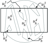
Figure 5: Illustration of another application. The biggest rectangle denotes the query range $R$. The uncertainty region $u$ is a closed region with 7 holes.

Additional observations. To compute $u$, the method in Section IV-C is using $e$ to subtract each candidate restricted area $r$ on by one. Consider the case $r\subset e$. Clearly, $e-r$ forms a polygon with hole. For ease of discussion, let $e^{\prime}$ be the subtraction result between $e$ and $r$, and assume that the next candidate restricted area to be processed is $r^{\prime}$. The natural approach is using $e^{\prime}$ to subtract $r^{\prime}$. This approach however, complicates the follow-up computation, and thus incurs extra overhead. This is mainly because geometrical operation on polygons with holes is generally more complicated and time consuming than on polygons without holes. To overcome this drawback, we employ a postpone processing mechanism. Specifically, if $r\subset e$, we postpone the subtraction operation by caching $r$ in a temporary place; after all other candidate restricted areas are handled, we finally fetch $r$ from the temporary place and then handle it. For instance, in Figure 4(b) we handle $r_{3}$ and $r_{7}$ at last.

Another common case is that $r$ intersects with $e$ but $|e-r|=1$, where $|\cdot|$ denotes the number of subdivisions. To this case, the natural method is using $e$ to subtract $r$, and then update the MBR of this subtraction result. This approach is inefficient, due to two main reasons: (i) such a new MBR usually does not make enough contribution to the rest of computation, i.e., its pruning power is weak in most cases; (ii) to obtain such a new MBR also needs to traverse the vertexes of this subtraction result, which incurs the extra overhead. To overcome this drawback, we employ a lazy update mechanism. Specifically, if $|e-r|=1$ (i.e., no multiple subdivisions appear), we only execute the subtraction operation but do not update the MBR of the subtraction result. $r_{4}$ in Figure 4(b) illustrates this case, for example. We remark that the two mechanisms above can be directly applied to the case of computing $s$. For instance, see Figure 5, the lazy update can be applied to $u_{h}^{3}$, and the postpone processing can be applied to $u_{h}^{1}$.

VI Precomputation based method

In the previous discussion, we assume a twin-index is adopted: $\mathscr{I}_{r}$ is used to manage restricted areas, and $\mathscr{I}_{o}$ is used to manage moving objects. Once a moving object $o$ reports its new location to the server, we update its recorded location $l_{r}$, and also update $\mathscr{I}_{o}$. (See Section IV-E.) An obvious characteristic of this method is to compute uncertainty regions on the fly, and an easily brought to mind method is to incorporate the precomputation strategy.

Simply speaking, we index restricted areas at first, and then precompute uncertainty regions and index them. Here we also adopt a twin-index. One is used to manage restricted areas, which is the same as the previous. Another, called $\mathscr{I}_{u}$, is used to manage the uncertainty regions. Specifically, for each moving object $o$, we search its candidate restricted areas on $\mathscr{I}_{r}$, and then compute its uncertainty region $u$ and index it using $\mathscr{I}_{u}$.

Note that, it is possible that an object $o$ reports its new location to the server in the process of constructing $\mathscr{I}_{u}$. To this issue, we differentiate two cases: (i) the uncertainty region of this object $o$ has ever been precomputed and indexed; and (ii) the uncertainty region of this object $o$ has not been precomputed. Both of the cases can be tackled easily. For instance, regarding to the first case, we can update its recorded location $l_{r}$ in the database, and then recompute its uncertainty region and update the current $\mathscr{I}_{u}$ right now. For the second case, we only need to update its recorded location $l_{r}$ in the database for the present. Once the precomputation is accomplished, the query can be executed, which is the similar as the previous. Henceforth, if an object $o$ reports its new location to the server, we also compute its uncertainty region (off-line) and update $\mathscr{I}_{u}$. Note that although the precomputation based solution seems to be more efficient, it however has a (non-trivial) drawback, i.e., its preprocessing time is rather large, which will be demonstrated in the next section.

VII Performance study

VII-A Experiment settings

Datasets. In our experiments, both real and synthetic datasets are used. Two real datasets are named as CA and LB, respectively. The CA contains 104770 2D points, and the LB contains 53145 MBRs. We use the CA to denote recorded locations of moving objects, and the LB to denote restricted areas. In order to simulate moving objects with different characteristics, we randomly generate different distance thresholds (from 20 to 50) for them. The size of 2D space is fixed at 10000$\times$10000, all datasets are normalized in order to fit this size of 2D space. Synthetic datasets also include two types of information. We generate a number of polygons to denote restricted areas, and let them uniformly distributed in 2D space. We generate a number of points to denote recorded locations of moving objects, and let them randomly distributed in 2D space. Note that, there is an extra constraint — these points cannot be located in any restricted area. We use the RE and SY to denote the real and synthetic datasets, respectively.

Methods. Existing methods are invalid to our problem, we thus do not compare with them. The straightforward method is infeasible and difficult to implement, as analysed in Section III, we thus do not discuss this method in our experiments (we believe the readers can understand this situation). Specifically, we implemented our solution (Section IV), our solution together with the optimization (Section V), and the precomputation based solution together with the optimization (Section VI). We use the same indexing structure, R-tree, for the three algorithms above. For brevity, we use S, SO, and PSO to denote them, respectively. Furthermore, by the convention, we implemented a baseline method that is to do a linear scan when searching candidate moving objects and candidate restricted areas (note: other strategies are the same as the ones of the S). We use B to denote it for short.

Distributions. In our experiments, two types of PDFs are used: uniform distribution and distorted Gaussian (note: our solutions can also work for other distribution PDFs, since we adopt the Monte Carlo method that can work for arbitrary distribution PDF). The definition of distorted Gaussian is based on the general Gaussian. Let $pdf_{G}(x,y)$ and $pdf_{DG}(x,y)$ be the PDFs of general Gaussian and distorted Gaussian, respectively, and let $\lambda$ be a coefficient, where $\lambda=\int_{\forall(x,y)\in u}pdf_{G}(x,y)dxdy$, we have

$$pdf_{DG}(x,y)= \frac{pdf_{G}(x,y)}{\lambda}, (x,y)\in u$$ if (21a)

$$pdf_{DG}(x,y)= 0,$$ otherwise (21b)

In theory, we should have calculated $\lambda$ and converted $pdf_{G}(x,y)$ into $pdf_{DG}(x,y)$ for each object $o$. Fortunately, we need to neither calculate $\lambda$, nor do any conversion. This is because $\lambda$ will be eliminated when we substitute $pdf_{DG}(x,y)$ with $\frac{pdf_{G}(x,y)}{\lambda}$ in the following formula.

$$p=\frac{\sum_{i=1}^{N_{2}}{pdf_{DG}{(x_{i},y_{i})}}}{\sum_{i=1}^{N_{1}}{pdf_{DG}{(x_{i},y_{i})}}}$$ (22)

where $N_{1}$, $N_{2}$ are the number of random points being located in $u$ and $s$, respectively. For brevity, we use UD and DG to denote uniform distribution and distorted Gaussian, respectively.

Metrics. The performance metrics in our experiments include: the I/O time, query time (the sum of I/O and CPU time), preprocessing time and accuracy. We use the workload error to measure the accuracy. Two types of common workload errors are the relative workload error (RWE) and absolute workload error (AWE). In order to investigate I/O and query time, we randomly generate 50 query ranges, and run 10 times for each test, and finally compute the average I/O and query time for estimating a single query. We run 10 times and compute the average value for estimating the preprocessing time. In order to get the workload error, we generate an object $o$ at the centre of the $2$D space, and assign a value to the distance threshold $\tau$, and then compute its uncertainty region $u$. Next, we generate 100 query ranges that have the same size, but have different intersections with $u$. At first run, we get the real answer of each query by setting $N^{\prime}=1e+7$. (We remark that an absolute real answer is unavailable, since the Monte Carlo method itself is an approximation algorithm. Even though, this obtained answer can be almost regarded as the real value, as we assign a very large number to $N^{\prime}$. In the rest of the paper, we slightly abuse the term “real value”.) Next, we vary the size of $N^{\prime}$ to get several groups of workload errors. We note that another parameter $\xi$ also results in workload errors. When we study the impact of $\xi$ on the accuracy, we also use the workload error to estimate the returning results. The test method is similar to the one used to test $N^{\prime}$. Specifically, we get the real answer of each query by setting $\xi=32^{2}$, then vary $\xi$ to get several groups of workload errors.

Para.	Description	Value
$\xi$	number of edges of $e$	[$16,24,\textbf{32},48,64,32^{2}$]
$N$	cardinality of $\mathscr{O}$	[$10k,20k,30k,40k,\textbf{50k}$]
$M$	cardinality of $\mathscr{R}$	[$10k,20k,30k,40k,\textbf{50k}$]
$\theta$	size of $R$	[$100,200,300,400,\textbf{500}$]
$\zeta$	number of edges of $r$	[$\textbf{4},8,16,32,64$]
$N^{\prime}$	number of random points	[$600,\textbf{700},800,900,5k,6k,10^{7}$]
PDF	distribution in $u$	[ UD, DG ]
$\tau$	distance threshold of $o$	[$20,21,\cdots,49,50$]

TABLE II: Parameters Used in Our Experiments

Parameters. All codes used in our experiments are written in C++ language; all experiments are conducted on a computer with 2.16GHz dual core CPU and 1.86GB of memory, running Windows XP. The page size is fixed to 4096 bytes; the maximum number of children nodes in the R-tree is fixed to 50. The standard deviation of $pdf_{G}(x,y)$ (used for defining $pdf_{DG}(x,y)$) is set to $\frac{\tau}{5}$, the mean $u_{x}$ and $u_{y}$ are set to $l_{r}.x$ and $l_{r}.y$, respectively, where ($l_{r}.x$, $l_{r}.y$) denote the coordinates of $l_{r}$.

The settings of other parameters are illustrated in Table II, in which the numbers in bold represent the default settings. $N$, $M$ and $\zeta$ refer to the settings of synthetic datasets, the default setting of each restricted area $r$ is a rectangle with $40\times 10$ size, and the one of the query range $R$ is a rectangle with $500\times 500$ size.

VII-B Results

VII-B1 Choose the error metric and the size of $N^{\prime}$

Recall Section VII-A that there are two error metrics, both of them can be used to measure the accuracy. Note that, to ensure a small RWE takes more time (a non-trivial number) than to ensure a same value of AWE. The results shown in Figure 6(a) confirm this fact. These results are derived by setting $\tau=20$. In this figure, the AWE is $0.95\%$ (i.e., 0.0095) and the RWE is $10.75\%$, when $N^{\prime}=700$. It is unreasonable if we choose $10.75\%$ as the RWE. Otherwise, it implies that returning a value of $89.25\%$ will be tolerated even if the real value is $100\%$. Therefore, we need to increase $N^{\prime}$ in order to get a smaller RWE. By doing so, we get RWE$=1.12\%$ and AWE$=0.05\%$ at $N^{\prime}=50000$. Therefore, if we want to assure a value $1\%$ of RWE, we have to set $N^{\prime}>50000$ at least. However, even if we let $N^{\prime}=50000$, and only compute a single object’s probability, it takes about 2871 milliseconds, implying that to assure a small RWE (e.g., $1\%$) takes much time. To further verify this fact, we conduct another set of experiments using both real and synthetic datasets where we set $N^{\prime}=50000$ and others are the default settings. The results are listed in the table below.

Dataset.	Total test time (sec.)	Query time (sec.)
RE	21399.25	427.985
SY	166022.6	332.004

The total test time takes about 59 and 46 hours, respectively; and each single query takes several minutes. In view of these, and in most cases a small AWE is enough to satisfy our demand, in the rest of experiments we choose to assure a small AWE by setting $N^{\prime}$ to a smaller value. Figure 6(b) depicts the results by setting $\tau$ to 20, 30, 40 and 50, respectively. We can see that on the whole, an object with a smaller $\tau$ usually needs a larger $N^{\prime}$, if we want to assure the same value of AWE. Based on the facts above, unless stated otherwise, we choose $N^{\prime}=700$ in the rest of experiments, which can ensure a value 0.01 of AWE.

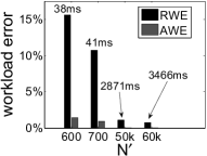
(a) AWE and RWE vs. $N^{\prime}$

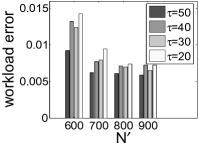
(b) AWE vs. $\tau$ and $N^{\prime}$

Figure 6: Workload Error Comparison.

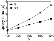
(a) SY dataset (query time)

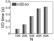
(b) SY dataset (I/O time)

Figure 7: Query and I/O performance vs. $N$.

VII-B2 S vs. SO

We first study the impact of $N$, $M$ and $\zeta$ based on synthetic datasets, and then study the impact of $\theta$ and $\xi$ based on both real and synthetic datasets.

Impact of $N$. Figure 7 illustrates the results by varying $N$ from 1e$+4$ to 5e$+4$. We can see that with the increase of $N$, both the query and I/O time increase for the two methods. In terms of query performance, we find that the SO outperforms the S, which demonstrates the efficiency of our optimization. In particular, their performance differences are more obvious especially when $N$ is large, which demonstrates the scalability of SO is better than the one of S. We remark that the I/O performance of the two methods is identical, this is because same location and restricted area records are fetched from the database for the two methods. In the rest of experiments, we only report the IO performance of SO.

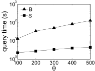
(a) SY dataset (query time)

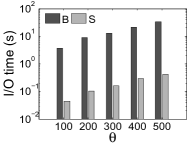
(b) SY dataset (I/O time)

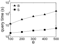
(c) RE dataset (query time)

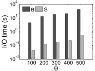
(d) RE dataset (I/O time)

Figure 8: Query and I/O performance vs. $\theta$.

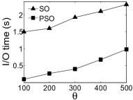
(a) SY dataset (query time)

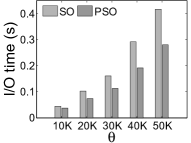
(b) SY dataset (I/O time)

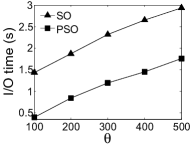
(c) RE dataset (query time)

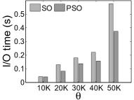
(d) RE dataset (I/O time)

Figure 9: Query and I/O performance vs. $\theta$.

VII-B3 B vs. S

We can see from Figure 8 that both the query and I/O performance of the S significantly outperform the ones of B. Note that when we vary other parameters in addition to $\theta$, we also get similar results, i.e., the S significantly outperforms the B. Clearly, the SO also significantly outperforms the B as it is superior than the S.

VII-B4 SO vs. PSO

From Figure 9, we can see that the PSO outperforms the SO regardless of query or I/O performance, which demonstrates the benefits of precomputing uncertainty regions. Note that we also vary other parameters and find that the PSO also outperforms the SO in terms of query and I/O performance.

However, we find that the time for precomputing uncertainty regions is rather long, the results are plotted in Figure 10. The PSO takes 2532.828 seconds (about 42 minutes) when the default settings of the synthetic datasets are used (note: the SO do not need to precompute uncertainty regions, and only need to index restricted areas and moving objects, which can be finished in several seconds). In addition, when we set $\zeta$ to 64, the PSO takes 5386.812 seconds (about an hour and a half). The long preprocessing time can be regarded as a (non-trivial) drawback of this approach.

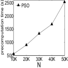
(a) SY dataset

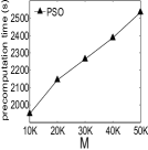
(b) SY dataset

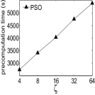
(c) SY dataset

Figure 10: Precomputation time vs. $N$, $M$ and $\zeta$.

VII-B5 Compare different PDFs

We next test the impact of PDFs. Specifically, we let all parameters be totally same except the PDF (note: here we use our preferred method, i.e., the SO). On one hand, we compare their query time by varying $\theta$ (here $N^{\prime}$ is the default setting). On the other hand, we compare their accuracies by varying $\xi$ (here we set $N^{\prime}$ to $10^{7}$).

Query time. Figure 11(a) and 11(b) depict the results when we vary $\theta$. We can see that the query time when the PDF is DG is more than the one when the PDF is UD. This is mainly because the time computing a single object’s probability is relatively long when the PDF is DG.

Accuracy. In addition, by varying $\xi$ from 16 to 64, their accuracies are plotted in Figure 12(a). As we expected, the larger (the) $\xi$ is, the more accurate answer we can get. In particular, we can see that, compared to the case of uniform distribution, $\xi$ makes less impact on the accuracy when the PDF is DG. Hearteningly, even if the PDF is UD, the accuracy of the proposed method is still high since the AWE is about 634$\times 10^{-6}$ when $\xi=32$. Moreover, we can see from Figure 12(b) that, with the same $\xi$, the smaller the distance threshold $\tau$ is, the more accurate answer we can get when the PDF is UD. Interestingly, the case of DG is exactly the opposite, which confirms (in a different way) the previous conclusion derived from Figure 6(b). Furthermore, we also report the RWEs of the set of experiments, which are shown in Figure 12(c) and 12(d), respectively. By comparing Figure 12(a)/12(b) and Figure 12(c)/12(d), we can easily see that in the same settings, the AWE is significant smaller than the RWE, which is in line with the conclusion derived from Figure 6(a).

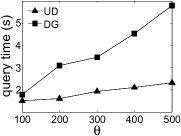
(a) SY dataset (query time)

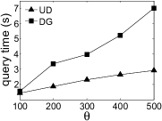
(b) RE dataset (query time)

Figure 11: Query efficiency vs. PDF.

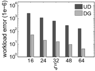
(a) AWE vs. $\xi$ ($\tau=50$)

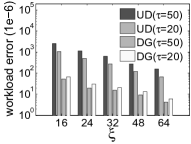
(b) AWE vs. $\tau$ and $\xi$

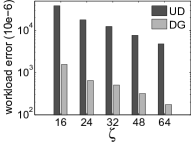
(c) RWE vs. $\xi$ ($\tau=50$)

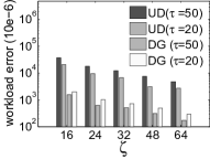
(d) RWE vs. $\tau$ and $\xi$

Figure 12: Accuracy vs. PDF.

VIII Conclusion

This paper studies the CSPRQ for uncertain moving objects. The deliberate analyses offer insights into the problem considered, and show that to process the CSPRQ using a straightforward method is infeasible. We propose the targeted solution and demonstrate its efficiency and effectiveness through extensive experiments. An additional finding is the precomputation based method has a non-trivial preprocessing time (although it outperforms our preferred solution in other aspects), which offers an important indication sign for the future research. We conclude this paper with several interesting research topics: (i) how to process the CSPRQ in 3D space? (ii) if the location update policy is the time based update, rendering that the uncertainty region $u$ is to be a continuously changing geometry over time, how to process the CSPRQ in such a scenario? (iii) if the query issuer is also moving, the location of query issuer is also uncertain, how to process the location based CSPRQ?

References

- [1] M. D. Berg, O. Cheong, M. V. Kreveld, and M. Overmars. Computational geometry: algorithms and applications, Third Edition. Springer, Berlin, 2008.
- [2] B. Braden. The surveyor’s area formula. The College Mathematics Journal, 17(4):326–337, 1986.
- [3] J. Chen and R. Cheng. Efficient evaluation of imprecise location dependent queries. In IEEE International Conference on Data Engineering (ICDE), pages 586–595. 2007.
- [4] R. Cheng, D. V. Kalashnikov, and S. Prabhakar. Querying imprecise data in moving object environments. IEEE Transactions on Knowledge and Data Engineering (TKDE), 16(9):1112–1127, 2004.
- [5] B. S. E. Chung, W.-C. Lee, and A. L. P. Chen. Processing probabilistic spatio-temporal range queries over moving objects with uncertainty. In International Conference on Extending Database Technology (EDBT), pages 60–71. 2009.
- [6] T. Emrich, H.-P. Kriegel, N. Mamoulis, M. Renz, and A. Züfle. Querying uncertain spatio-temporal data. In IEEE International Conference on Data Engineering (ICDE), pages 354–365. 2012.
- [7] B. Gedik, K.-L. Wu, P. S. Yu, and L. Liu. Processing moving queries over moving objects using motion-adaptive indexes. IEEE Transactions on Knowledge and Data Engineering (TKDE), 18(5):651–668, 2006.
- [8] G. Greiner and K. Hormannn. Efficient clipping of arbitrary polygons. ACM Transactions on Graphics (TOG), 17(2):71–83, 1998.
- [9] K. Hormann and A. Agathos. The point in polygon problem for arbitrary polygons. Computational Geometry, 20(3):131–144, 2001.
- [10] H. Hu, J. Xu, and D. L. Lee. A generic framework for monitoring continuous spatial queries over moving objects. In ACM International Conference on Management of Data (SIGMOD), pages 479–490. 2005.
- [11] B. Kuijpers and W. Othman. Trajectory databases: Data models, uncertainty and complete query languages. Journal of Computer and System Sciences (JCSS), 76(7):538–560, 2010.
- [12] Y. K. Liu, X. Q. Wang, S. Z. Bao, M. Gombosi, and B. Zalik. An algorithm for polygon clipping, and for determining polygon intersections and unions. Computers and Geosciences (GANDC), 33(5):589–598, 2007.
- [13] A. Margalit and G. D. Knott. An algorithm for computing the union, intersection or difference of two polygons. Computers and Graphics, 13(2):167–183, 1989.
- [14] H. Mokhtar, J. Su, and O. H. Ibarra. On moving object queries. In International Symposium on Principles of Database Systems (PODS), pages 188–198. 2002.
- [15] D. Pfoser and C. S. Jensen. Capturing the uncertainty of moving-object representations. In International Symposium on Large Spatial Databases (SSD), pages 111–132. 1999.
- [16] A. Rappoport. An efficient algorithm for line and polygon clipping. The Visual Computer (VC), 7(1):19–28, 1991.
- [17] A. P. Sistla, O. Wolfson, S. Chamberlain, and S. Dao. Modeling and querying moving objects. In IEEE International Conference on Data Engineering (ICDE), pages 422–432. 1997.
- [18] Y. Tao, X. Xiao, and R. Cheng. Range search on multidimensional uncertain data. ACM Transactions on Database Systems (TODS), 32(3):15, 2007.
- [19] G. Trajcevski, A. N. Choudhary, O. Wolfson, L. Ye, and G. Li. Uncertain range queries for necklaces. In International Conference on Mobile Data Management (MDM), pages 199–208. 2010.
- [20] G. Trajcevski, O. Wolfson, K. Hinrichs, and S. Chamberlain. Managing uncertainty in moving objects databases. ACM Transactions on Database Systems (TODS), 29(3):463–507, 2004.
- [21] B. R. Vatti. A generic solution to polygon clipping. Communications of the ACM (CACM), 35(7):56–63, 1992.
- [22] H. Wang and R. Zimmermann. Processing of continuous location-based range queries on moving objects in road networks. IEEE Transactions on Knowledge and Data Engineering (TKDE), 23(7):1065–1078, 2011.
- [23] O. Wolfson, A. P. Sistla, S. Chamberlain, and Y. Yesha. Updating and querying databases that track mobile units. Distributed and Parallel Databases (DPD), 7(3):257–387, 1999.
- [24] K.-L. Wu, S.-K. Chen, and P. S. Yu. Incremental processing of continual range queries over moving objects. IEEE Transactions on Knowledge and Data Engineering (TKDE), 18(11):1560–1575, 2006.
- [25] M. Zhang, S. Chen, C. S. Jensen, B. C. Ooi, and Z. Zhang. Effectively indexing uncertain moving objects for predictive queries. The Proceedings of the Very Large Database Endowment (PVLDB), 2(1):1198–1209, 2009.
- [26] K. Zheng, G. Trajcevski, X. Zhou, and P. Scheuermann. Probabilistic range queries for uncertain trajectories on road networks. In International Conference on Extending Database Technology (EDBT), pages 283–294. 2011.