Mean-field learning: a survey
Abstract
In this paper we study iterative procedures for stationary equilibria in games with large number of players. Most of learning algorithms for games with continuous action spaces are limited to strict contraction best reply maps in which the Banach-Picard iteration converges with geometrical convergence rate. When the best reply map is not a contraction, Ishikawa-based learning is proposed. The algorithm is shown to behave well for Lipschitz continuous and pseudo-contractive maps. However, the convergence rate is still unsatisfactory. Several acceleration techniques are presented. We explain how cognitive users can improve the convergence rate based only on few number of measurements. The methodology provides nice properties in mean field games where the payoff function depends only on own-action and the mean of the mean-field. A learning framework that exploits the structure of such games, called, mean-field learning, is proposed. The proposed mean-field learning framework is suitable not only for games but also for non-convex global optimization problems. Then, we introduce mean-field learning without feedback and examine the convergence to equilibria in beauty contest games, which have interesting applications in financial markets. Finally, we provide a fully distributed mean-field learning and its speedup versions for satisfactory solution in wireless networks. We illustrate the convergence rate improvement with numerical examples.
1 Introduction
Recently there has been renewed interest in large-scale games in several research disciplines, with its uses in financial markets, biology, power grid and cloud networking. Classical work provides rich mathematical foundations and equilibrium concepts, but relatively little in the way of learning, computational and representational insights that would allow game theory to scale up to large-scale systems. The literature on learning in games with discrete action space is huge (see [1, 3, 30] and the references therein). However, only few results are available for continuous action space. In this paper, we explain how the rapidly emerging field of mean-field games can address such behavioral, learning and algorithmic issues.
We propose both model-based (but still with less information) and non-model-based learning schemes for games with continuous action space and large number of players. Each player will update her learning strategies based on an aggregative term [15], which is the sum of action of the other players. Each player will be influenced by the aggregate, and the mean field behavior is formed from the contributions of each player. In the model-based mean-field learning scheme, the mean action will be read by the players at each time slot, and each player will respond to the aggregative term locally. This simplifies drastically the dimensionally of the best-response system in the asymptotic case.
We distinguish different types of learning schemes depending on the information requirement:
(i) Partially distributed strategic learning [30], where each player knows her own-payoff function, has some computational capabilities and observes the actions of the other players at the previous step. Examples of such learning schemes include best response algorithms, fictitious play, and logit algorithms.
(ii) Fully distributed strategic learning: In many dynamic interactions, one would like to have a learning and adaptive procedure which does not require any information about the other players actions or payoffs and less memory as possible (small number of parameters in term of past own-actions and past own-payoffs). Fully distributed learning algorithms are only based on numerical measurements of signals or payoffs. The mathematical structure of own-payoff functions are not assumed to be known by the player. Hence, gradient-like ascent and best-reply algorithms cannot be used directly. The observations of private signals/measurements are not explicit in the actions of the other players. Based on numerical measurement of realized own-payoff, each player employs a certain learning pattern in order to learn the expected payoff function (payoff-learning) as well as the associated optimal strategies (model-free strategy-learning). This type of learning algorithm is referred as Combined fully DIstributed PAyoff and Strategy learning (CODIPAS, [29, 31, 2]). These algorithms are simple but they play an important role in terms of applications since they are based on experiments and real data. In the continuous action space case, the gradient of own-payoff is not observed and hence it needs to be estimated or learned if one wants to use a gradient-like ascent method. However, estimating an accurate gradient based only on a sequence of payoff measurements is not a trivial task.
(iii) No-feedback learning where the players do not observe any numerical payoff measurement. These schemes are based only on estimations and offline adjustment. However, conjectures and hierarchical reasoning could be used in order to get consistent reactions.
In all the above three categories of learning algorithms, the combination of the learning patterns of all the players form a multidimensional interactive system. The question we address is whether it is possible to exploit the structure of the payoff functions in large-scale regime to reduce the complexity of the above learning algorithms (partially or fully distributed).
The answer to this question is positive for some aggregative games. We examine three classes of mean-field learning frameworks:
-
•
Partially distributed mean-field learning where each player knows her own-payoff function, has some computational capabilities and observes the mean field at the previous step. Examples of such learning algorithms include best response to mean field and Boltzmann-Gibbs mean-field response.
-
•
Fully distributed mean-field learning schemes can be used in situations where each generic player in the large population is able to observe/measure a numerical value of her own-payoff (that could be noisy). These schemes are derivative-free and model-free. They can be applied in both mean-field games and mean-field global optimization.
-
•
No-feedback mean-field learning: There are some situations where it is difficult to feedback any information to the population of players and local measurement of own-payoff is not available. Then, the above two classes of learning algorithms that are based on feedbacks to the players are inappropriate. In that case, a learning scheme without feedback can be employed if the payoff functions are common knowledge.
1.1 Overview: learning for games with continuous action space
We briefly overview fully distributed learning for games with continuous action space. One of the first fully distributed learning algorithms is the so-called reinforcement learning. While there are promising results in Markov decision processes with few number of states and actions, majority of reinforcement Q-learning, adaptive heuristic critic, and regret minimizing multi-arm bandit algorithms meet several difficulties in continuous action space. The difficulty in extending such learning algorithms to multi-player games is that with a balance has to be maintained between exploiting the information gained during learning, and exploring the set of actions (with is a continuum) to gain more information. Instead of updating a finite dimensional probability vector, one has to adjust a probability density function in infinite dimensional space. The authors in [32] has proposed reinforcement learning algorithms for games with continuous and compact action space applied to vehicle suspension control. The convergence analysis is not conducted in [32] .
In [33] the authors studied continuous action reinforcement learning automata and applied to adaptive digital filters. The authors claimed convergence of their algorithm via computer simulations.
Recently, [34] observed a poor performance and selection of basis functions that are used in [32, 33] to approximate the infinite dimensional space. It is conjectured that the convergence time (when it converges) is very high even for quadratic cost function.
In order to reduce the dimensionality, the basic idea in these continuous action space reinforcement learning studies has been to use a normal distribution at each time slot and updates the mean and standard deviation based on the payoff measurement.
Another approach to continuous action space learning is the regret minimizing procedure that allows to be close to the Hannan set. Such a procedure have been widely studied for discrete action space and has several interesting computational properties: the set of correlated equilibria is convex and there is polynomial time algorithm. The extension to continuous and compact action space has been conducted in [35]. It is shown that the empirical frequencies of play converges to the set of correlated equilibria. However, most of these convergence results are not for a point but a set and the convergence time is not provided in [35]. Another important point is that the convergence of the frequency of play does not imply the convergence of actions or strategies. All the above references consider finite number of players.
In this work we are interested on learning in games with large number of players and continuous action space. The framework presented here differs from classical machine learning for large-scale systems. The main difference is the strategic behavior of the players who make decisions in a distributed and autonomous manner. This creates an interdependency between the decisions through the mean of the mean-field.
1.2 Contribution
Our contributions can be summarized as follows. First, we introduce a learning framework for games with large population of players, called mean-field learning. Considering payoff functions that depend on own-input and an aggregative term, we show that mean-field learning simplifies drastically the analysis of large-scale interactive learning systems. In the single class case, it reduces to the analysis of one iterative process instead of an infinite collection of learning processes. Second, we study both asymptotic [40] and non-asymptotic properties of the resulting learning framework. Stability, error bounds and acceleration techniques are proposed for model-based mean-field learning as well as for derivative-free mean-field learning. In particular, we show that the convergence time of order speedup learning is at most
where is the error target, is a positive value which does not depend on time and is the initial error gap. Interestingly, the methodology extends to satisfactory solution (which is a situation where all the players are satisfied). We provide fully distributed mean-field learning schemes for satisfactory solution in specific games. Reverse Ishikawa and Steffensen speedup learning are proposed to improve the convergence rate to satisfactory solution. Numerical examples of the basic learning techniques are illustrated and compared in guessing games and in quality-of-service (QoS) satisfaction problems in wireless networks.
1.3 Structure
The paper is organized as follows. In the next section we present a generic mean-field game model. In Section 3 we present the mean-field learning framework. In Section 4 we present a detailed example of beauty contest mean-field game. Speedup strategic learning for satisfactory solution are presented in Section 5. Finally, section 6 concludes the paper.
The proofs are given in Appendix.
2 Mean field game model
Consider players. Each player takes her action in the convex set Denote the set of players by In the standard formulation of a game, a player’s payoff function depends on opponents’ individual actions. Yet, in many games, payoff functions depend only on some aggregate of these, an example being the Cournot model where it is the aggregate supply of opponents that matters rather than their individual strategies. The main property of aggregative games is the structure of the payoff functions. The payoff function of each player depends on its own action and an aggregative term of the other actions. A generic payoff function in aggregative game with additive aggregative term is given by
| (1) |
where the actions are real numbers and In this context the key term of player is the structure of the function , its own-action and the aggregative term
The triplet constitutes a one-shot game in strategic form.
Applications 1
The type of aggregate-driven reward function in (1) has wide range of applications:
(a) In economics and financial markets, the market price (of products, good, phones, laptops, etc) is influenced by the total demand and total supply,
(b) In queueing theory, the task completion of a data center or a server is influenced by the mean of how much the other data centers/servers can serve.
(c) In resource sharing problems, the utility/disutility of a player depends on the demand of the other players. Examples include cost sharing in coalitional system and capacity and bandwidth sharing in cloud networking.
(d) In wireless networks, the performance of a wireless node is influenced by the interference created by the other transmitters.
(e) In congestion control, the delay of a network depends on the aggregate (total) flow and the congestion level of the links/routes.
Definition 1
The action profile is a pure equilibrium of the game if no player can improve her payoff by unilateral deviation i.e., for every player one has
Before going for pure equilibrium seeking we first need to ask if the problem is well-posed, i.e; the existence of a pure equilibrium. Below we provide a classical sufficiency condition for existence of a pure equilibrium in continuous-kernel aggregative games.
The following results hold:
-
•
compactness: If is a non empty, compact, convex subset of , and each is (lower semi-) continuous in and quasi-concave with the respect to the first variable then possesses at least one pure strategy Nash equilibrium.
-
•
If is non-compact, we require additional coercivity assumption: as
For discontinuous payoff function we refer to the recent development of existence of pure equilibria. A very active area is the full characterization for the existence of pure strategy Nash equilibrium in games with general topological strategy spaces that may be discrete, continuum or non-convex and payoff functions that may be discontinuous or do not have any form of quasi-convexity. For more details, see the literature review in Tian (2009, [13]).
Below we examine only the cases in which the game admits at least one equilibrium and the best-response is uniquely given by the mapping (which is not necessarily continuous). We present aggregate-based learning algorithms. Generically, a partially distributed mean-field-based learning scheme can be written as where is specified from the game model and is a mean action of the players at time In this paper we examine only schemes with one-step memory in the form
2.1 Aggregate-based best-response
Let be the mean of actions of the others. We assume that has a unique element which we denote by Then, is the best-response map. We aim to find a fixed-point of such a map in which is in an Euclidean space with dimension Exploiting the aggregative structure of the game and the convexity of the set the domain of the function is reduced to the set by the following relation where by convexity of the domain The simultaneous best-response algorithm, called mean-field response, is given in Algorithm 1 which requires that player observes the common term at the previous step and computes
2.2 Banach-Picard learning algorithm
One of the first basic iterative procedures for finding fixed-point of the continuous map over complete metric space is the Banach-Picard iterate. The algorithm consists to start at some point and take the compositions that is , where This algorithm is known to be convergent for strict contraction map, i.e., if there exists a Lipschitz constant of the function then the iterates converge (with geometric convergence rate ) to the unique fixed-point of in However, in many applications of interest the function may not be a contraction. See Example 1 below.
Theorem 1 ([5])
Let be a complete metric space, and a map for which there exist real numbers and satisfying such that for each pair in , at least one of the following conditions is true:
Then, the Banach-Picard algorithm converges to a fixed-point of for any initial point Moreover, has a unique fixed-point.
Note that the first part of Theorem 1 C0 has many applications in solving nonlinear equations, but suffers from one drawback - the contractive condition (C0) forces to be continuous on However, the second condition (C1) does not require continuity of the best response function The condition (C1) have been studied by Kannan (1968, [12]) and (C2) by Chatterjea (1972, [11]).
Example 1 (Resource sharing game)
Consider players in a network with a resource capacity Each player has a certain demand which corresponds to her action. The action space is Denote by the unit price for each resource utilization. The payoff function is
where is a positive parameter. Then, the (simultaneous) best-response algorithm is given by
and
A direct computation of the derivative (at the interior) gives
Clearly, is not a contraction.
Example 2
A non-convergent Banach-Picard iteration is obtained for and is Lipschitz in the domain Let start with then The two subsequences and have different limits. Hence, the sequence does not converge if the starting point is
We explain below how to design a convergent sequence for the problem of Examples 1 and 2. A simple modification of Banach-Picard consists to introduce a learning rate which takes the average between the previous action and the best response, Then, the procedure evolves slowly. The idea goes back at least to Mann (1953, [8]) and Krasnoselskij (1955, [7]). For equal to one, one gets the Banach-Picard algorithm.
If the function satisfies (Lipschitz and strongly pseudo-contractive map)
for any pair where and there is such that for any , the learning algorithm converges to a fixed-point. However, for closer to one, the algorithm may oscillates around a fixed-point. In order to get a smaller in the long-run, we can attempt to take a decreasing learning rate as grows.
The algorithm (also referred to as Mann’s algorithm [8]) reads
| (2) | |||
| (3) |
If the function does not satisfy one can still get some convergence results due to Ishikawa [10, 9].
| (4) | |||
| (5) | |||
| (6) |
Clearly, the same technique can be extended to a finite number of compositions of the mapping
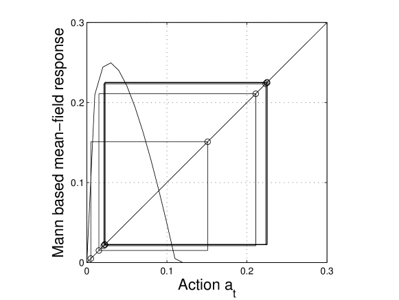
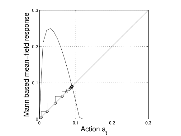
Figure 1 illustrates a cycling behavior of the mean-field response of example 1. The parameters are For smaller than the one in Figure 1, the cycle disappeared and the Ishikawa’s based mean-field response scheme behaves well. See Figure 2.
2.3 Faster algorithms: Banach-Picard vs Ishikawa
For a class functions satisfying one of the conditions C0-C2, we know from Theorem 1 that there is a unique fixed-point of and the speed of convergence of the algorithm can be compared for different parameter Suppose that and are two real convergent sequences with limits and respectively. Then is said to converge faster than if
The authors in [6, 5] showed that for a particular class of functions that satisfies one of the conditions C0, C1 or C2, the Banach-Picard algorithm is faster than the Ishikawa’s algorithm with is faster than the one with However in general these algorithms are not comparable due to non-convergence. For example for there is a unique fixed point but Banach-Picard does not converge starting from However, the Ishikawa method converges to for small enough.
2.4 Reverse Ishikawa mean-field learning
The reverse Ishikawa’s mean-field learning consists to choose a learning rate (bigger than one) that converges to one.
| (7) | |||
| (8) |
Example of could be When convergent, this scheme has the advantage of being faster than the fixed-point iteration.
2.5 Non-asymptotic properties
We focus on the non-asymptotic properties of the Ishikawa-based learning algorithms. Non-asymptotic strategic learning is very important in engineering applications. Traditional results on the fundamental limits of data compression and data transmission through noisy channels apply to the asymptotic regime as codelength, blocklength goes to infinity. However, these asymptotic results are not usable if the window size and horizon are bounded. Therefore, it is interesting to look at the non-asymptotic regime of learning algorithms. We provide generic rate of convergence of some class of best-response functions.
2.5.1 Strict contraction
For strict contraction mapping with constant , one has the following estimates:
The advantage of this inequality is that it provides a error gap at any time which is a non-asymptotic learning result.
2.5.2 Nonexpansive best-response function
The next result provides the convergence rate of the asymptotic regularity for nonexpansive maps i.e., the class of map with Lipschitz constant Denote by the diameter of the set
Theorem 2 ([4])
Let is a nonexpansive self-mapping of a bounded convex subset of a normed linear space, normalized so with non-empty fixed-point set the Ishikawa algorithm with and is a proper convex combination then
Moreover
If is unbounded, the following estimate holds:
We observe that when one gets the so-called asymptotic regularity of the sequence generated by the Ishikawa algorithm.
2.5.3 Strongly pseudocontractive
Theorem 3 ([14])
Let Lipschitz with constant and strongly pseudocontractive with constant such that is non-empty. Then the Ishikawa algorithm with converges strongly to the (unique) fixed point of The convergence rate is geometric and is given by
where
which is minimized for
2.6 Asymptotic pseudo-trajectories
Using classical approximation the asymptotic pseudo trajectories of Ishikawa’s algorithm can be studied using ordinary differential equations (ODEs). We assume that the function has a unique integral curve, in order to guarantee the uniqueness of the ODE (given a starting point).
2.6.1
The ODE is given by
which is the aggregate-response dynamics in continuous time.
If denotes a best response of then the steady state of the aggregate-response dynamics are Nash equilibrium of the aggregative game. If the dynamics has a Lyapunov function then one gets a global convergence to Nash equilibria. These games are called Lyapunov games.
Now we turn to the convergence time for a given error/precision. We define the convergence time of within a neighborhood as the first time the trajectory of pure strategy reaches a neighborhood of range to the set of fixed-points.
2.6.2 How to accelerate the convergence time of the ODE?
Consider the ordinary differential equations (ODEs) that captures the trajectories of the learning pattern in transient phase: and Assume that the two ODEs start at the same point What can we say about the trajectories of and
We explicitly give the convergence time of in function of that of
Proposition 1
The explicit solution is given by
In particular, if the trajectory of reaches a target set for at most time units then the trajectory of reaches the same set for at most where
If then
If then i.e., goes to zero and is faster than
3 Mean-field learning
We now consider a continuum of players. The mean-field is the action distribution Its mean is in the set and is denoted by Then the limiting payoff for single class writes All the functions above are reduced a single function i.e., each player responds to the mean of the mean-field. Therefore the Banach-Picard (mean-field response) dynamics becomes
which can be reduced to
| (9) |
by indistinguishability property.
Thus, Banach-Picard-based mean-field response learning is given by
| (10) |
Note that in Equation (10) only the starting point is required if the player knows the structure of This means that it is not needed to feedback the mean of the mean-field at each step.
Proposition 2
Consider a mean field game such the mean field response function is a strict contraction mapping over (non-empty, convex subset of ) with constant . Then, the mean-field response learning (10) finds an approximated fixed-point within a neighborhood in at most number of iterations where
The Ishikawa-based mean field response is
| (11) | |||
| (12) | |||
| (13) |
Based on Theorem 2, the next Proposition provides an upper bound of the convergence time in order of
Proposition 3
Consider a mean field game such the mean field response function is a nonexpansive mapping over (non-empty, convex subset of ). Then, the Ishikawa based mean-field learning (11) finds an approximated fixed-point within an neighborhood in at most number of iterations where .
Proposition 4 provides a convergence time bound in order of for Lipschitz with constant and strongly pseudocontractive mean-field response function
Proposition 4
Let Lipschitz with constant and strongly pseudocontractive with constant such that is non-empty. Then the Ishikawa algorithm with converges strongly to the (unique) fixed point of with at most number of iterations where
3.1 How to accelerate the convergence rate?
We have seen in the previous sections that under suitable conditions one can approximate fixed-points. However, the major concern associated with the above fixed-point iteration is that the iterates exhibit only linear convergence rate which may be unacceptably slow.
Speedup strategic learning is a method that studies learning mechanisms for speeding up the convergence based on few experiences. The input to a speedup technique typically consists of observations of prior realized sequence of experience, which may include traces of the measurements of the real problem. The output is knowledge that the technique can exploit to find solutions more quickly than before and without seriously effecting solution quality.
Our motivation for speedup learning is two-fold:
-
•
Traditional results on the fundamental limits of data compression and data transmission through noisy channels apply to the asymptotic regime as codelength, blocklength goes to infinity. However, these asymptotic results are not usable if the window size and horizon are bounded. Speedup strategic learning is aimed exclusively at finding solutions in a more practical time frame. Therefore, it is interesting to look at the non-asymptotic regime using speedup learning algorithms.
-
•
Speedup strategic learning aims to create adaptive scheme that can learn patterns from few number of experience that can be exploited for efficiency gains. Such adaptive schemes have the potential to significantly outperform traditional learning schemes by specializing their behavior to the characteristics of the fixed-point problem.
Consider a convergent mean-field learning with exhibit a sequence Suppose now that only few number of the sequence are available to the users. Each user aims to learn an approximate fixed-point based only minimal number of information about the estimates The goal of a generic user is to accelerate the previous learning algorithm and transform the slowly converging sequence into a new one that converge to the exact limit as the first one, but faster. If possible, we aim to be as close as possible to based only on the observations of the sequence .
Definition 2
Assume that converges to and let If If two positive constants exist, and
then the sequence is said to converge to with order of convergence . The number is called the asymptotic error constant. The cases are given special consideration.
(i) If the convergence of is called linear.
(ii) If the convergence of is called quadratic.
(iii) If the convergence of is called cubic.
3.1.1 Partially distributed speedup methods
We present speedup learning in one-dimensional space. However, most of the speedup schemes below extends to multi-dimensional action spaces.
Quadratic order speedup techniques
The basic Newton method consists to iterate
| (14) |
If and then the Newton’s method generates a quadratic convergence rate locally: where is in a neighborhood of and
For multiple roots, the scheme can be modified to be
or apply the Newton method to the function
3.1.2 Cubic order speedup techniques
One of the most studied cubic technique is the Halley’s method which consists to update as
3.1.3 Arbitrary order speedup techniques
We start with Householder’s speedup method [27]. If the map is known by the player then the classical fixed-point iteration is A order speedup learning is given by
where is an integer and is the derivative of order of the inverse of the function .
It is well-known that if is a times continuously differentiable function and is a fixed-point of but not of its derivative, then, in a neighborhood of , the iterates satisfy:
for some constant which is obtained by taking the bound of the derivatives of the function at The bound is finite because of continuity over compact set. This means that the iterates converge to the fixed-point if the initial guess is sufficiently close, and that the convergence has rate Thus, if is an infinitely differentiable function, this scheme makes a very fast locally convergent speedup learning algorithm with arbitrary high order. In particular, for this is the Newton’s method, for it is called Halley’s method.
For the case where the function is smooth with a unique fixed-point, we can systematically generate, high order, quickly converging, mean-field learning methods, of any desired degree, for the solution of fixed-point problem. Fast converging mean-field learning methods like those should be of great use in large-scale algorithms that require the repetitive solution of a nonlinear equation many times over long time periods and where an efficient solution algorithm is imperative to avoid overtime computations. This reduces the so-called cost of impatience, i.e., the cost due to the error gap to the solution. We now present our main result on the convergence time of the -order speedup scheme.
Theorem 4
Let and and Then the scheme is convergent and the error at iteration is bounded by
Thus, the convergence time to an range of the pure mean-field equilibrium is
where
3.1.4 Derivative-free speedup methods
The most well known sequence transformations are Aitken’s process (1926,[18]), Richardson’s extrapolation algorithm (1927, [23]), Shanks transformation (1955,[22]), Romberg transformation 1955 [19], Wynn’s algorithm (1956, [25, 26]). These speedup techniques are not based on derivatives. This is why they are used more frequently in practical computations.
Next we present a superlinear order derivative-free speedup technique, called Secant method. It is inspired from Newton’s method where the term replaces the derivative.
Secant speedup method
In the Secant speedup method (Algorithm 4), we define the sequence using two initial guesses, and and the formula:
| (15) |
which can be obtained when replacing by in Equation (14). Note that the Secant method can be written as which is a two-step memory scheme, since two previous values are required to calculate the next value in the sequence. The Secant speedup method converges with order around i.e., more quickly than a method with linear convergence, but more slower than a method with quadratic convergence.
Aitken’s speedup method
The new sequence that accelerates the convergence via Aitken extrapolation is
which is obtained by solving the equation
Steffensen’s speedup method
Steffensen’s speedup method (Algorithm 5) is a variant of the Aitken method that uses the Aitken formula to generate a better sequence directly:
Remark 1
Sometimes one has attempted to compare Newton, Secant, Aitken and Steffensen speedup methods. So, which method is faster? Ignoring constants, it would seem obvious that Newton’s method (model-based speedup technique) is faster than Secant method (non-model speedup technique), since it converges more quickly. However, to compare performance, we must consider both computational cost and speed of convergence. An algorithm that converges quickly but takes a few seconds per iteration may take far more time overall than an algorithm that converges more slowly, but takes only a few milliseconds per iteration. So, the comparison is not fair. For the purpose of this general analysis, we may assume that the computational cost of an iteration is dominated by the evaluation of the function. So, the number of function evaluations per iteration is likely a good measure of cost. The secant method requires only one function evaluation per iteration (the function ), since the value of can be stored from the previous iteration. Newton’s method requires one function evaluation and one evaluation of the derivative per iteration. It is difficult to estimate the cost of evaluating the derivative in general. In some cases, the derivative may be easy to evaluate, in some cases, it may be much harder to evaluate than the function (if it is possible at all). If we can run two iterations of the secant speedup method in the time it will take to run one iteration for computing the derivative in Newton’s method. Then, two iterations of the Secant speedup method should be compared to Newton’s speedup method. But Secant method with two iterations has a speedup in order of hence faster than the Newton’s method.
The Aitken speedup method requires three consecutive terms of the sequence to reproduce a quadratically convergent speedup technique.
3.2 Fully distributed derivative-free mean field learning
We now present a fully distributed mean-field learning based on the work of [24]. Each generic player adjusts its action based on numerical measurement of own-payoff (with some i.i.d noise). The first order learning scheme with large number of players is given in Algorithm 6.
where
Let From Taylor expansions and In the first order sinusoidal learning, the error rate is proportional to the second derivative (Hessian of the payoff). Since the payoff function is unknown to the players, it is difficult to tune the convergence rate with the appropriate parameters. Therefore, we estimate the Hessian and construct a dynamics that converge asymptotically to the pseudo-inverse of the Hessian. The local behaviour of the second order sinusoidal learning will be independent of the Hessian which is of big importance in non-model learning where the Hessian is unknown. The second order sinusoidal perturbation mean-field learning is given in Algorithm 7.
where
The product of needs to generate an estimate of the Hessian in a time-average sense and should generate an estimate pseudo-inverse of the Hessian. Example of function is
3.3 Feedback-free mean-field learning
Below we develop a learning algorithm without feedback (no mean-field feedback, or other actions at the previous step are not observed, [16]) but with knowledge of the mathematical structure of the payoff function. Feedback-free mean-field learning is very important and is therefore empirically testable. In it, players think that others are likely to take the some function of actions as themselves, resulting in a false consensus or non-false consensus depending on one’s view of the irrationality of the behavior and incompatibility of beliefs and conjectures.
A simple example of feedback-free learning consists to take a speedup version of starting from some estimate of the initial point and iterate offline.
Mean-field global optimization
Consider the average payoff in the form which is in general, not concave in the joint action. The asymptotic regime is which can be analyzed using measure theory. In particular, if the integral can be written as a function of only the first moment of the mean-field , i.e., then the above mean-field learning schemes can be used to learn the mean-field social optimum.
Example 3
We consider the payoff function in the following form: Then total payoff of all the players is where is the total sum of actions. By dividing by one gets
The dimensionality of the global optimization problem can be significantly reduced to be one-dimensional, i.e., It suffices to optimize the function The local extrema of this scalar function can be found using the above techniques.
This means that a mean-field optimization can be conducted easily for any limiting function in the form of where ’s are real numbers and are limiting functions of the mean of the mean-field.
In next section, we apply mean-field learning and speedup techniques in beauty contest game or guessing game.
4 Beauty contest game
We revisit the beauty contest game in the context of mean-field. The name of this game and its basic idea go back to John Maynard Keynes (1936) who compared a clever investor to a participant in a newspaper beauty-contest where the aim was to guess the average preferred face among 100 photographs. The initial beauty contest game was analyzed for integers, although in 1993 the German economist Rosemarie Nagel based her experiments on a nice variant of the game, played by Keynes’ newspaper readers: Each player chooses a real number between 0 and 100 inclusively. The number need not be an integer. A player wins if its number is closest to 2/3 of the average of the numbers given by all participants.
There are two ways to see that a unique equilibrium solution exists. First, one can easily see that no one should submit a number higher than 66, because whatever the others do, a guess higher than 66 cannot be better than 66. However, if no one guesses more than 66, then all numbers between 44 (that is, two third of 66) and 66 are inferior to 44. Hence no one would guess more than 44 and so on. until 0 is the only remaining reasonable choice. (Note that a second solution besides 0 is 1 if only integers are allowed).
A second method would be to just try out: Presume you guess a certain number , and anyone else guesses the same number , would you still wish to stick to your initial guess ? If so, you have found a symmetric Nash equilibrium. Now the only to which you would want to stick is
More generally, in a beauty contest game, players simultaneously choose numbers in some interval, say, The average of their numbers is computed, which establishes a target number where is a parameter. The player whose number is closest to the target wins a prize The generic payoff is
This model of beauty contest games were studied experimentally by Nagel (1995, [17]).
These games are useful for estimating the number of steps of iterated dominance players use in reasoning through games. To illustrate, suppose . Since the target can never be above , any number choice above is stochastically dominated by simply picking . Similarly, players who obey dominance, and believe others do too, will pick numbers below so choices in the interval violate the conjunction of dominance and one step of iterated dominance. We iterate this progressively and get that , then the unique Nash equilibrium is 0. Now, if then the equilibrium is If every feasible symmetric action profile is an equilibrium.
We now consider a small modification of the guessing game in order to get interior equilibria. The target is changed to be The generic payoff is
where
In the asymptotic regime, the interior mean-field equilibrium (if any) should satisfy i.e., in the interval
Assuming that the functions are known, we can use a feedback-free mean-field learning. Therefore, one possible explanation of no-feedback learning in the beauty contest game (or guessing game) is that players simply take an action, treat their action as representative of the choices of other players, and then best respond to this belief mean of the mean-field. This kind of reasoning would predict convergence towards equilibrium in the guessing game.
The best response dynamics is given by where the starting point is Each trader starts with an estimate It is clear that for if each trader estimates the initial point and iterate the mean-field learning process offline, the process converges to the mean-field equilibrium. For the interior response writes
More generally, one can consider a mean-field payoff in the following form
where is map which has a fixed point in The best response to the mean is and the mean-field pure equilibrium satisfies Hence, learning the mean-field equilibrium reduces to learning a fixed-point of the maping For the iterative process becomes Note that is a fixed-point. Let fix the starting point at and
We start with and use the secant speedup method. The result of acceleration technique (15) is presented in Table 1. We observe that at the fourth iteration, the secant speedup method has already of precision while the original sequence has a times smaller precision. Next we start with the initial point for secant method and initial point of for the fixed point method. We observe that the secant method has better precision than the fixed-point method after only iterations. This means that the secant speedup method is robust to initial estimation errors.
We summarize the acceleration technique in Table 2 based only on few steps of the original sequence.
Assume that only measurements of the mean sequence is given to the player: We apply the acceleration technique from these measurements and one gets
and
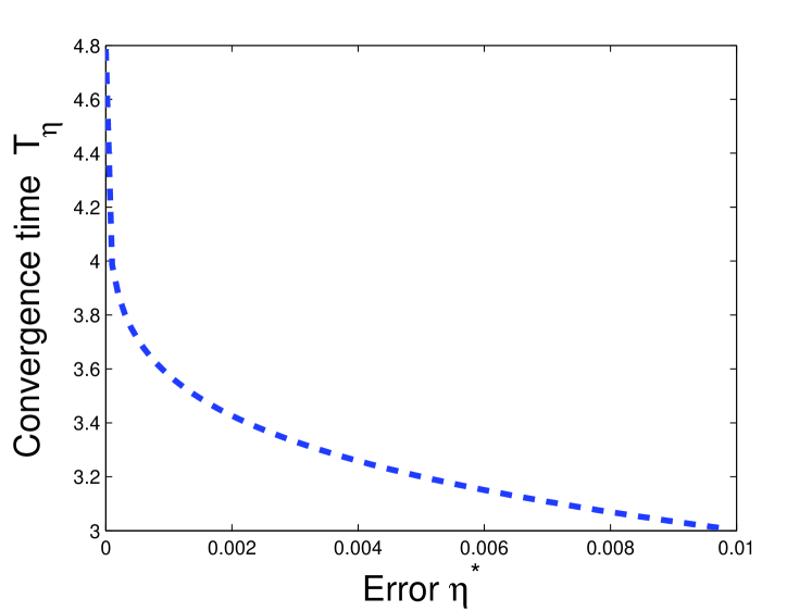
Clearly, the Aitken sequence guarantees that will converge faster to and the error will be smaller than that of the original sequence If we reiterate the fixed-point of the sequence but starting from the sequence Then, Repeating the acceleration procedure and taking the fixed-point iteration, one gets The sequence seems converges to with at least quadratic convergence rate which is great acceleration from the linear convergence rate of the original sequence. With only two iterations of Steffensen’s speedup method one has reached an error of which is satisfactory. In Figure 3 we illustrate the bound of Theorem 4 which states the convergence time with error We observe that the result of Figure 3 are similar to the one obtained in Table 2.
5 Speedup strategic learning for satisfactory solution
One of the fundamental challenges in distributed interactive systems is to design efficient and fair solutions. In such systems, a satisfactory solution is an innovative approach that aims to provide all players with a satisfactory payoff anytime anywhere. Our motivations for satisfactory solution seeking are the following: In dynamic interactive system, most users constantly make decisions which are simply “good enough” rather than best response or optimal. Simon (1956, [36]) has adopted the word “satisficing” for this type of decision. Most of literature of strategic learning and decision making problems, however, seek only the optimal solution or Nash equilibria based on rigid criteria and reject others. As mentioned by Simon himself in his paper in page 129, “Evidently, organisms adapt well enough to ’satisfice’; they do not, in general, ’optimize’. Therefore satisfactory solution offers an alternative approach and is closely model the way humans and cognitive users make decisions [37, 38, 39].
Here, a satisfactory strategy is a decision-making strategy that attempts to meet an acceptability threshold. This is contrasted with optimal decision-making or best response strategy, an approach that specifically attempts to find the best option available given the the choice of the other users. Following that idea we define a satisfaction solution as a situation where every user is satisfied, i.e., her payoff is above her satisfactory level.
In this section we focus on fully distribution strategic learning for satisfactory solution in games with continuous action space. For discrete (and finite) action space we refer to [20]. We show that the methodology in [20] can be extended to continuous action space as well as to first moment mean-field games. We illustrate it with a basic example. See also [21].
Definition 3
The action profile is a pure satisfactory solution of the game if all the players are satisfied:
Before going for pure satisfactory solution seeking we first need to ask if the problem is well-posed, i.e; the existence of a pure satisfactory solution.
We assume feasibility, that is, are chosen such that the set is nonempty. This means that there exists a vector such that there is an action profile that satisfies Thus, a necessary and sufficient condition for existence of a satisfactory solution is that the vector belongs to the set i.e., the range of the function
Consider a basic wireless network with users. The action space is There is a state space where The payoff of user in state is the signal-to-interference-plus-noise ratio: where is the background noise and To goal of each player is not necessarily to maximize the payoff, it is to get a certain target
Definition 4
We say that user is satisfied if
A satisfactory solution at state is a situation where all the users are satisfied. Such a situation may not exist in general. We examine the case where there is at least one solution. Of course if the full state and all the parameters are known, one can perform a centralized solution. However, in the distributed setting, a user may not have access to the information of the other users channel gains and their locations. Thus, it is important to guarantee a certain quality-of-service (QoS) with minimal information for all the users. Our goal here is to develop very fast and convergent fully distributed learning algorithms for satisfactory solutions. The only information assumption required to each user is the numerical realized value its own-payoff and its own-target The basic Banach-Picard fixed-point iteration is given by
where denotes the projection operator over the convex and compact set i.e.,
Note that and
The proposed algorithm is fully distributed in the sense that a user do not need to observe the actions of the others in order to update its strategy iteratively.
Next we discuss the convergence of the Banach-Picard learning algorithm for a fixed state
Assumption A0: where and
It is clear that under assumption A0, the system where has a solution. We say that the problem is feasible if has a solution and the solution satisfies
Proposition 5
Consider the Banach-Picard learning algorithm for a fixed state for which the problem is feasible.
-
•
Suppose that the sequences of action profiles generated by the Banach-Picard algorithm converges to some point that belongs to be relative interior of Then, is a satisfactory solution.
-
•
Under the sufficient condition for existence A0 and feasibility condition, the Banach-Picard iteration converges to a satisfactory solution.
-
•
The convergence rate of the Banach-Picard algorithm for satisfactory solution seeking is geometrical decay and hence the convergence time within error tolerance is
where
Remark 2 (Advantages)
This proposition is very important since a satisfactory solution can be seen as a global optimum of the game with payoff function where denotes the indicator function. In particular, the above algorithm is a fully distributed learning scheme that converges (under the existence and feasibility condition) to a global optimum (and hence Pareto optimal) which is remarkable.
Remark 3 (Limitations)
The fully distributed Banach-Picard algorithm proposed above is convergent under some range of parameters, and the algorithm is with minimal information (it is fully distributed). However, the convergence time is still unsatisfactory. We aim to investigate whether it is possible to get a faster convergence rate. To do so, we use speedup learning techniques.
One of the first speedup techniques for satisfactory solution is the reverse Ishikawa’s learning consists to choose a learning rate (bigger that one) that converges to one.
| (16) | |||
| (17) |
Theorem 5
Under the same assumption as in Proposition 5 and appropriate choice of the reverse Ishikawa learning converges faster than the Banach-Picard learning.
Note that the projection is now required even if is convex because for one gets is a not convex combination. In general, it is difficult to compute in advance the value of that will maximize the rate of convergence.
In order to get a higher order convergence rate, one can use a Steffensen speedup learning of the reverse Ishikawa.
Remark 4
In the above speedup learning for satisfaction, we have limited ourselves to the case where the state is quasi-static. However, in wireless networks, it could be stochastic, leading to a stochastic learning algorithm. Then, the goal is to find satisfactory solution in expectation. For that case, the assumption on is too restrictive. The spectral radius of the matrix may not be less than one for some realized state Then, a feasible solution may not exist but the algorithm converges to
In the context of large-scale games, one needs to scale the SINR. By choosing the parameter and independent of one can express the payoff of a generic user as function of and a load factor Therefore, the mean-field learning version becomes
| (18) | |||||
| (20) | |||||
Thus, and is an interior satisfactory solution and the payoff of a each generic player is
The reverse Ishikawa is
| (21) | |||||
| (22) | |||||
| (24) | |||||
For one can observe compare the spectral radius: Thus, the reverse Ishikawa learning has a superlinear convergence rate faster than the Banach-Picard fixed point iteration.
We choose the target SINR to be the scaled background noise and the load is and Then, the problem is feasible and the satisfactory solution is In table 3 we illustrate the convergence to satisfactory solution: Banach-Picard and its speedup versions with reverse Ishikawa and Steffensen. We initialize the mean of the mean field and observe that iterations of the Banach-Picard learning corresponds approximately to 25 iterations of the reverse Ishikawa learning and only iterations of Steffensen speedup algorithm.
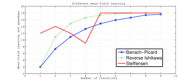
Figure 4 summarizes the three mean-field learning trajectories.
The satisfactory solution estimated by Banach-Picard mean-field is and the the error estimate for in the Banach-Picard learning is after iterations. The first speedup technique based on reversed Ishikawa with gets after iterations which clearly a superlinear convergence rate. The error estimate of reverse Ishikawa speedup is after iterations starting from which is far away from the satisfactory solution. We can get a higher order convergence rate. The speedup technique à la Steffensen provides an error of after only iterations. The numerical gap is in order of which is an acceptable error tolerance for 6 iterations.
6 Concluding remarks
In this paper we have studied mean-field learning in large-scale systems. Our result shows that in large-scale aggregative games with additive aggregation term, the mean-field learning simplifies not only the complexity of the problem (instead of systems of iterative equations, we can just reduce to one-equation per class or type) but also the information requirement. We have examined both convergence time and speed of convergence and proposed acceleration techniques for partially distributed mean-field learning with convergence time in order of
In the fully distributed mean-field learning, we have assumed that each player is able to observe/measure a noisy (numerical) value of her payoff in a linear way. Now, what happens if this assumption does not hold but a correlated non-linear signal is observed as output? After an experimentation at time player observes the realized process where is the observation function and is the measurement noise. If the observation function is binary then one gets a output or a noisy ACK/NACK feedback. If is known and invertible with the respect to the first component, one can use a non-linear mean field estimator to track the “true” payoff function simultaneously with the strategy. As a third alternative, we have seen that no-feedback mean-field learning is possible. In it, each player estimates the initial mean and iterates offline without any observation/signal from the system. Several questions remain open:
(i) In the mean-field learning without feedback, How to estimate the starting point by each player and what is the impact on the inconsistency of the process with the respect to the mean-field?
(ii) What is the outcome of the mean field game if some fraction of players are with partially distributed learning, some fraction with fully distributed learning schemes and some others without any feedback learning?
(iii) How to extend the mean-field learning framework to payoff functions that depend not only on the mean also but on higher moments or the entire mean-field distribution?
(iv) Our analysis of speedup learning algorithms are limited to deterministic function. It is interesting to investigate the stochastic version of (8).
We do not have answers to these questions and postpone them for future investigation.
References
- [1] Sergiu Hart, Andreu Mas-Colell: Stochastic uncoupled dynamics and Nash equilibrium. Games and Economic Behavior 57(2): 286-303 (2006)
- [2] M. Khan, H. Tembine, A. Vasilakos, Game Dynamics and Cost of Learning in Heterogeneous 4G Networks, IEEE Journal on Selected Areas in Communications, vol 30, 1, pp 198 - 213, January 2012, special issue on Game Theory in Wireless Communications.
- [3] Roberto Cominetti, Emerson Melo, Sylvain Sorin: A payoff-based learning procedure and its application to traffic games. Games and Economic Behavior 70(1): 71-83 (2010)
- [4] J. Baillon, R.E. Bruck, The rate of asymptotic regularity is , in: Theory and applications of nonlinear operators of accretive and monotone type, Lecture Notes in Pure and Appl. Math. 178, Dekker, New York, pp. 51-81 (1996).
- [5] T. Zamfirescu, Fix point theorems in metric spaces, Archiv der Mathematik 23 (1992), 292298.
- [6] Babu, G.V.R., Vara Prashad K.N.V., Mann iteration converges faster than Ishikawa iteration for the class of Zamfirescu operators, Fixed Point Theory and Applications Vol. 2006, Article ID 49615,
- [7] Krasnoselskij, M.A., Two remarks on the method of successive approximations (Russian) Uspehi Mat. Nauk. 10 (1955), no. 1 (63),123-127
- [8] W. R. Mann, Mean value methods in iteration, Proc. Amer. Math Soc., 4 (1953), pp. 506-510.
- [9] S. Ishikawa, Fixed points and iteration of a nonexpansive mapping in a Banach space, Proc. American Mathematical Society, 59(1) (1976).
- [10] Ishikawa, S., Fixed points by a new iteration method Proc. Amer. Math. Soc. 44 (1974), No. 1, 147-150.
- [11] Chatterjea, S. K., Fixed-point theorems, C.R. Acad. Bulgare Sci. 25 (1972), 727-730.
- [12] Kannan, R. Some results on fixed points, Bull. Calcutta Math. Soc. 10 (1968), 71-76.
- [13] Guoqiang Tian, 2009. The Existence of Equilibria in Games with Arbitrary Strategy Spaces and Payoffs: A Full Characterization, Levine’s Working Paper Archive 814577000000000160,
- [14] V. Berinde and M. Berinde, The fastest Krasnoselskij iteration for approximating fixed points of strictly pseudo-contractive mappings, CarpathianJ. Math. 21 (2005), No. 1 - 2, 13 - 20.
- [15] Dubey, P. and A. Mas-Colell, and M. Shubik (1980): Efficiency Properties of Strategic Market Games: An Axiomatic Approach, Journal of Economic Theory 22, 339-362. 25
- [16] Weber, Roberto A. ’Learning’ with no feedback in a competitive guessing game, Games and Economic Behavior, 44,1,134-144, JUL 2003
- [17] Nagel, R., 1995. Unraveling in Guessing Games: An Experimental Study. American Economic Review 85(5): 1313-1326.
- [18] A. C. Aitken, On Bernoulli’s numerical solution of algebraic equations, Proc. Roy. Soc. Edinburgh, 46 (1926), 289-305.
- [19] W. Romberg, Vereinfachte numerische Integration, Norske Vid. Selsk. Forh., 28 (1955), 30-36.
- [20] S. M. Perlaza , H. Tembine, S. Lasaulce, and M. Debbah, Satisfaction Equilibrium for Quality-Of-Service Provisioning in Decentralized Networks, IEEE Journal on Selected Topics in Signal Processing. Special Issue in Game Theory for Signal Processing, 2012.
- [21] H. Tembine, R. F. Tempone, P. Vilanova, Mean-field learning for satisfactory solutions, 2012.
- [22] D. Shanks, Non-linear transformations of divergent and slowly convergent sequences, J. Math. and Phys. (Cambridge, Mass.), 34 (1955), 1-42.
- [23] L. F. Richardson, The deferred approach to the limit. I: Single lattice, Philos. Trans. Roy. Soc. London, Ser. A, 226 (1927), 299-349.
- [24] S.-J. Liu and M. Krstic, Stochastic Nash equilibrium seeking for games with general nonlinear payoffs, SIAM Journal of Control and Optimization, vol. 49, pp. 1659-1679, 2011
- [25] P. Wynn, Acceleration technique for iterated vector and matrix problems, Math. Comp., 16 (1962), 301-322.
- [26] P. Wynn, On a device for computing the em(Sn) transformation, MTAC, 10 (1956), 91-96.
- [27] A. S. Householder, The Numerical Treatment of a Single Nonlinear Equation, McGraw-Hill, New York, (1970)
- [28] H. P. Young. Strategic learning and its limits. Oxford University Press, 2004.
- [29] R. Bush and F. Mosteller. Stochastic models of learning. Wiley Sons, New York., 1955.
- [30] H. Tembine, Distributed strategic learning for wireless engineers, CRC Press, Taylor & Francis Inc., 2012.
- [31] H. Tembine, Dynamic robust games in MIMO systems, IEEE Transactions on Systems, Man, Cybernetics, Part B, 99, Volume: 41 Issue:4, pp. 990 - 1002, August 2011.
- [32] M. N. Howell, G. P. Frost, T. J. Gordon, and Q. H. Wu. Continuous action reinforcement learning applied to vehicle suspension control. Mechatronics, 7(3):263–276, 1997.
- [33] M.N. Howell, T.J. Gordon, Continuous action reinforcement learning automata and their application to adaptive digital filter design, Engineering Applications of Artificial Intelligence 14 (2001) 549-561, Elsevier.
- [34] A. Rodriguez, R. Grau, and A. Nowe. Continuous action reinforcement learning automata. performance and convergence. In Joaquim Filipe and Ana Fred, editors, 3rd International Conference on Agents and Artificial Intelligence ICAART 2011, pages 473 - 478 January 2011.
- [35] G. Stoltz and G. Lugosi, (2007). Learning correlated equilibria in games with compact sets of strategies. Games and Economic Behavior, 59:187-208.
- [36] Simon, H. A. Rational choice and the structure of the environment. Psychological Review, Vol. 63 No. 2, 129-138, 1956.
- [37] Wynn C. Stirling, Satisficing Games and Decision Making With Applications to Engineering and Computer Science, 268 pages, Cambridge Univ. Press, 2003.
- [38] Michael A. Goodrich, Wynn C. Stirling, Richard L. Frost: A theory of satisficing decisions and control. IEEE Transactions on Systems, Man, and Cybernetics, Part A 28(6): 763-779, 1998.
- [39] Wynn C. Stirling, Michael A. Goodrich: Satisficing Games. Inf. Sci. 114(1-4): 255-280, 1999.
- [40] H. Tembine, J. Y. Le Boudec, R. ElAzouzi, E. Altman, Mean Field Asymptotic of Markov decision evolutionary games, International IEEE Conference on Game Theory for Networks, Gamenets 2009.
Proof of Theorem 4: Let We reiterate the recursive equation
| (25) | |||||
| (26) | |||||
| (27) | |||||
| (28) | |||||
| (29) |
We remember that for Thus,
This means that the convergence time to be within an neighorbhood of the mean-field equilibrium is at most for satisfying Thus,
By taking the logarithm twice, one gets
which is the announced result.
Proof of Proposition 2:
Using the strict contraction map we estimate the error at time and get
i.e.
Taking the logarithm yields,
This completes the proof.
Proof of Proposition 3:
To prove the convergence time of learning with non-expansive map, we use the Theorem 2. The error bound to an approximated fixed-point is
Remark that for Then, the convergence time is at most for a time that satisfies
Hence,
Proof of Proposition 4: The proof follows immediately from the geometric decay inequality in Theorem 3 following similar lines as in Proposition 2.
Proof of Proposition 1: Let The function is differentiable and the time derivative is
Moreover, By Cauchy’s theorem, Suppose now that reaches a target set with at most time units. Then, the trajectory of reaches the same set for at most where Since if and non-integrable then has a solution.
If then
If then i.e., goes to zero and is faster than
Proof of Proposition 5:
If the algorithm converges to a some point then combining the continuity of the projection map and the continuity of the payoff function, one gets the righthandside of
which is continuous in Taking the limit as goes to infinity, one gets or and the payoff of player is which means that every player is satisfied in interior steady state.
Now assume feasibility and assumption A0. Then, From Perron-Frobenius theorem, we known that exists and is positive componentwise. Under feasibility condition, the algorithm generates an error as
which provides the convergence of the algorithm to We use similar analysis as in Proposition 4 to deduce the convergence time
Proof of Theorem 5:
Following the proof of Proposition 5, one gets that there is some time such that for all the spectral radius of the time-varying matrix for is less that i.e., the reversed Ishikawa has a superlinear convergence rate. If then both algorithms converge to the same point and the reverse Ishikawa learning algorithm converges faster than the Banach-Picard fixed-point. The reverse Ishikawa is a speedup version of the Banach-Picard algorithm and the announced result follows.