Econoinformatics meets Data-Centric Social Sciences

Abstract

Our society has been computerised and globalised due to emergence and spread of information and communication technology (ICT). This enables us to investigate our own socio-economic systems based on large amounts of data on human activities. In this article, methods of treating complexity arising from a vast amount of data, and linking data from different sources, are discussed. Furthermore, several examples are given of studies into the applications of econoinformatics for the Japanese stock exchange, foreign exchange markets, domestic hotel booking data and international flight booking data are shown. It is the main message that spatio-temporal information is a key element to synthesise data from different data sources.

1 Introduction

Recently people feel data in various fields due to developments in information and communication technology (ICT). This circumstance enables us to collect, store, and analyse data on our socio-economic environment in order to interpret our society and to pursue evidence-based management. One can collect and accumulate large amounts of socio-economic data on human activities, and analyse and visualise them. Vast amounts of data collected from socio-economic systems have made new types of commercial services and research fields emerging. According to M.F. Goodchild [1], every human is able to act as an intelligent sensor, and in that sense, the earth’s surface is currently occupied by more than six billion sensors.

We can extract information from an amount of data, construct knowledge from lots of information, and hopefully establish wisdom from several pieces of knowledge. Specifically, researchers in the fields of sociology, economics, informatics, and physics are focusing on these frontiers and have launched data-centric social sciences in order to understand the complexity of socio-economic systems [2].

However, since our society which is the sum total of both internal and external states of individuals is several orders of magnitude more complicated than each individual, it seems difficult to image how we could manage to capture the real totality of its states with the cooperation of many agencies. The nature of this problem is referred to recognised as “complexity”, which is a new research field into knowledge on groups of people, organisations, communities, and the economy actually behave in the real world.

Information theory describes the number of possible states of a system as its “complexity”. Complexity may be estimated with Shannon information entropy or thermodynamic entropy. For example, researchers have used a methodology to characterise the structure of networks with information-theoretic entropy [3, 4]. According to a study by Dehmer and Mowshowitz [3], the concept of graph entropy was first proposed in the 1950s to measure structural complexity. Rashevsky [5], Trucco [6], and Mowshowitz [7] were the first researchers to define and investigate the entropy of graphs. Several graph invariants, such as the number of vertices, vertex degree sequence, and extended degree sequence, have been used in the construction of entropy-based measures. Wilhelm an Hollunder considered the normalised weight of the flux between two nodes as the probability of a symbol in the transmitter signal that corresponds to the sum of all influxes to/effluxes from a given node [4]. Sato also considered information-theoretic measures for a bipartite graph, and inferred economic situations using the network entropy of relative frequencies among group populations [8]. Bianconi looks at the entropy measure of network ensembles under several constraints [9, 10].

According to Heinz von Foerster [11], complexity is not a property which observed systems possess rather, it is to be perceived by observing systems. He asks us about it through the following question: Are the states of order and disorder states of affairs that have been discovered, or are their states of affairs that are invented? If states of order and disorder are discovered, then complexity is a property of the observed systems. If invented then it pertains to the observing systems. Foerster’s definition of complexity proposes that the relative degree of order and disorder is determined by the degrees of freedom of an observed system and an observing system. One of the most significant reasons that we recognise complexity in observed systems is because of the finiteness of periods when and abilities with which we are able to observe the systems, and the limitations of our memory and a priori knowledge of them that lead to our bounded rationality, or nescience.

From the data-centric perspective, complexity is referred to as a ratio of an amount of data to human cognitive capacity. How many megabytes of memory the human brain has? Von Neumann proposed that human memory is estimated as 100 exabits from all the neural impulses conducted in the brain during a lifetime [12]. Another method is to estimate the total number of synapses, and then presume that each synapse can hold a few bits. Estimates of the number of synapses have been made in the range from $10^{13}$ to $10^{15}$, with corresponding estimates of memory capacity. Landauer investigated how much people remember at Bell Communications Research [13]. The remarkable result of this work was that human beings remembered very nearly two bits per second under all the experimental conditions (visual, verbal, musical). Therefore, the 35-year accumulation of human beings’ memory estiamtes of 0.2 to 1.4 gigabits if the loss of memory are assumed.

If the amount of data is greater than this estimates of memory, then all the data can not be memorised by each human being. Therefore, the amounts of data may determine the complexity in the sense of the data accessiblity. This may provide a kind of definition of big-data in data-centric sciences.

Clearly, we also need to carefully consider methods of collecting, storing, handling, and analysing a vast amount of data in computer systems.

In this article, I present exemplar studies of observation and data analysis with a large amount of data in several socio-economic systems. I would like to call such studies “econoinformatics”. Econoinformatics needs powerful computer systems to visualise and quantify the behaviour of human beings, adapt to their changing environments, and evolve over time.

Furthermore, we should mention the problem of data linkage in data-centric studies. Data linkage is referred as to a method of linking data from different sources with the same elements. If we can synthesise data from different sources, we may find new insights from the synthesised data. The comprehensive study is further useful to obtain new findings on our environment.

The literature review on data-centric social sciences is provided in Section 2 of this article. In Section 3 exemplar studies on econoinformatics are shown. The Japanese stock exchange, the foreign exchange market, hotel booking data, and flight booking data are analysed. In Section 4, a method of synthesising data from different sources, and a method of econoinformatics, are discussed. Section 5 is devoted to conclusions.

2 Literature review

Recently, several researchers in a wide spectrum of fields have paid a remarkable amount of attention to massive amounts of comprehensive data. For example, search engines of web services need massive data about hyperlink connections among web pages, and electronic commerce systems need to cover information of various kinds of products. Due to the development of ICT, the Advanced Information Society has already emerged globally and it has gradually made our world smaller and smaller. The term “information explosion” has been coined to describe this situation and has been realised [14, 15]. This term refers to a situation in which the total amount of information created by individuals exceeds the individuals’ information processing capability.

Studies with vast amounts of socio-economic data have several branches. Here, five kinds of recent studies (financial market data, demographic data, traffic flow data, POS data, and e-commerce data) are surveyed for the purpose of finding ways of coping with the complexity of human societies.

A large amount of data on financial markets is available because the electronic matching systems of financial markets are spreading all over the world due to the development of ICT. Contemporary trading is done through electronic platforms, and settlement operations are done through electronic clearing systems. Financial market data can be collected through a direct application programming interface (API) or through the historical data centres of data providers. Applications of statistical mechanics to finance, by means of statistical physics, agent-based modelling, and network analysis, have progressed during the last decade [16, 17, 18, 19].

The launch of the E-Stat database by the Japanese government [20] provides us with new technological means for a data-based understanding of our country. In principle, everyone can understand the state of our country from demographic data. Furthermore, real-time demographic data are also available since the technologies to collect human activities via personal mobile phones have been established [21]. In the near future, we will be able to visualise real-time demographics, both comprehensively and circumstantially.

Recently, several car navigation companies have launched autonomous sensory navigation services in Japan. As a result, these companies can collect real-time car traffic data via each car navigation terminal. By collecting data from many cars, one can find roads and points where traffic jams are occurring. Without constructing new infrastructure to collect traffic states, real-time traffic data can be accumulated due to the development of Integrated Transport Systems (ITS). Based on such data, comprehensive analyses of traffic flows can be conducted in order to cope with traffic jams [22]. Recent developments in traffic measurement technologies have been driving the theoretical development of traffic control and modelling [23].

POS is an abbreviation for “point-of-sales”, and all department stores and supermarkets have introduced this kind of system in order to ring up purchases at cash registers. As a result, retail sales can be managed in real-time, and data-centric operations can be done. On the basis of these massive amounts of data, new marketing methods have been developed. The statistical properties of expenditure in a single shopping trip show a power-law distribution [24]. A comprehensive analysis of retail sales is one of the most promising directions to be followed in order to bridge the gap between microeconomics and macroeconomics.

Web-based commerce systems enable us to purchase everything, from books to electronic equipment, via websites. The details of consumers and goods can be stored on the data-base engine of each website. If we can use such data, then we may, in principle, capture real-time demand and supply of all items which are traded via websites. Analysing massive amounts of data on items which are sold via web commerce systems is expected to open a window to new economic theory and service engineering [25, 26]. Data on hotel booking opportunities [27], international flight booking opportunities [28], and price comparison sites [29] has also been studied.

The property that these studies seem to have in common is their ability to overcome the complexity in socio-economic systems, by using massive amounts of data and vast computations. Copious amounts of data on human activities are collected by means of ICT, and vast amounts of computation for such data are conducted for the purposes of searching, matching, visualising, and extracting.

3 Exemplar studies on econoinformatics

Large-scale data on socio-economic systems may make it possible to understand our society from a holistic point of view. To do so, we need to discuss the possibilities of comprehensive analysis and data linkage. In this section, four types of exemplar studies on socio-economic systems are shown. These examples include studies on the Japanese stock exchange, the foreign exchange market, hotel bookings through an e-commerce platform, flight bookings through an e-commerce platform. In order to archive a comprehensive point of view, both the Japanese and international economic situations are measured.

3.1 Japanese stock exchange

During the last two decades, it is said that the main problem faced by Japan is a low productivity growth rate. Despite these circumstances, the Japanese economy recovered eventually, with the aid of the global growth from 2004 to 2007. However, the latest global financial crisis strongly affected many countries, including Japan, after the midquarter of 2008. At that time, we observed that Japanese stock prices dropped sharply due to financial turmoil of 2008-2009. Furthermore, huge earthquakes hit Japan on 11 March 2011, and the Japanese economy suffered from a large number of social losses.

So far, we have explained the affairs by the Japan explanatory narrative. The question remains, however, as to how we can describe our macroeconomics situations in a more quantitative fashion.

Macroeconomic situations strongly influence money flows at all levels of society. Stocks at each sector are traded by investors and traders every minute through the stock exchange market. Moreover, stock prices are so sensitive to money flows, that stock prices in all sectors reflect demand-supply gaps of the money by economic actors. Therefore, they are expected to be useful for detecting changes in macroeconomic situations.

In this study, we hope to provide some insights on the problem of the quantification of Japanese macroeconomic situations, through a comprehensive analysis of stock prices traded in the Tokyo Stock Exchange. In the context of economics and finance, there are various methods available for segmenting highly nonstationary financial time series into stationary segments, called regimes or trends. Following the pioneering works of Goldfeld and Quandt [30], there is an enormous body of literature on detecting structural breaks or change points separating stationary segments. Recently, a recursive entropic scheme to segment financial time series was proposed [31].

In this study, a recursive segmentation procedure is applied to an analysis of security prices of 1,413 Japanese firms listed on the first section of the Tokyo Stock Exchange. The number of segments in quintiles in terms of variance is computed in order to detect change points of money flows of the Japanese security market.

Let $O_{i,t}$ and $E_{i,t}$ be daily opening and closing prices of $i$-th stock $(i=1,\ldots,M)$ at day $t\quad(t=1,\ldots,N)$. $M$ and $N$ are denoted as the total number of stock and the observation length. The daily log-return (opening to closing) time series $x_{i,t}\quad(i=1,\ldots,M;t=1,\ldots,n)$ is computed as $x_{i,t}=\log E_{i,t}-\log O_{i,t}$ and $n=N-1$.

According to the seminal work by Mantegna and Stanley [17], the log-return time series of stock prices are modelled by Lévy distributions. Superstatistics suggested that a mixture of Gaussian distributions with $\chi^{2}$-distributions in terms of variance gives a Lévy distribution. Therefore, we assume that each segment is sampled from a Gaussian distribution with different mean and variance. It is assumed that the log-return time series in segment $m_{i}$ follows a stationary Gaussian distribution with mean $\mu_{i,m_{i}}$ and variance $\sigma_{i,m_{i}}^{2}$.

To find the unknown segment boundaries $t_{i,m_{i}}$ separating segment $m_{i}$ and $m_{i}+1$, the recursive segmentation scheme introduced by Bernaola-Galván et al [31, 32] is employed. In this segmentation scheme, the likelihood of the total time series is compared with the likelihood of the two segmented time series.

Suppose that there are $n$ observations $x_{s}\quad(s=1,\ldots,n)$. Let $g(x;\mu,\sigma)$ be a Gaussian distribution:

$$g(x;\mu,\sigma^{2})=\frac{1}{\sqrt{2\pi\sigma^{2}}}\exp\Bigl{[}-\frac{(x-\mu)^{2}}{2\sigma^{2}}\Bigr{]},$$ (1)

Assuming that the observations $x_{s}$ should be segmented at $t$, and that the observations on the left hand side are sampled from $g(x;\mu_{L},\sigma_{L}^{2})$, and that those on the right hand side are from $g(x;\mu_{R},\sigma_{R}^{2})$, we define likelihood functions:

$$L = \prod_{s=1}^{n}g(x_{s};\mu,\sigma^{2}),$$ (2)

$$L_{2}(t) = \prod_{s=1}^{t}g(x_{s};\mu_{L},\sigma_{L}^{2})\prod_{s=t+1}^{n}g(x_{s};\mu_{R},\sigma_{R}^{2}).$$

Furthermore, we define the logarithmic difference between $L$ and $L_{2}(t)$ as,

$$\Delta(t)=\log L_{2}(t)-\log L.$$ (4)

Inserting Eq. (1) into Eq. (4), we have,

$$\Delta(t)=\sum_{s=1}^{t}\log g(x_{s};\mu_{L},\sigma^{2}_{L})+\sum_{s=t+1}^{n}\log g(x_{s};\mu_{R},\sigma^{2}_{R})-\sum_{s=1}^{n}\log g(x_{s};\mu,\sigma^{2}).$$ (5)

In general, if a random varialbe $A$ is given and its distribution admits a probability density function $f$, then the expected value of $A$ (if exists) can be calculated as

$$\mbox{E}[A]=\int_{-\infty}^{\infty}af(a)\mbox{d}a,$$ (6)

where $f(a)$ is a probability density function of $A$. This implies that the arithmetic mean of $m$ random variables $a_{i}\quad(i=1,\ldots,m)$ is approximated as

$$\frac{1}{m}\sum_{i=1}^{m}a_{i}\approx\int_{-\infty}^{\infty}af(a)\mbox{d}a,$$ (7)

for a sufficiently large value of $m$.

By using this approximation, for $m$ observations $x_{s}\quad(s=1,\ldots,m)$, we obtain

$$\sum_{s=1}^{m}\log g(x_{s};\mu,\sigma^{2})\approx m\int_{-\infty}^{\infty}g(x;\mu,\sigma^{2})\log g(x;\mu,\sigma^{2})\mbox{d}x=-\frac{m}{2}\log\Bigl{(}2\pi e\sigma^{2}\Bigr{)},$$ (8)

and $\Delta(t)$ is rewritten as,

$$\Delta(t)=n\log\sigma-t\log\sigma_{L}-(n-t)\log\sigma_{R}\geq 0.$$ (9)

$\Delta(t)$ can be used as an indicator to separate the observations into two parts. An adequate way to separate the observations is that a segmentation is conducted at $t$ where $\Delta(t)$ takes the maximum value. Namely, an adequate segmentation should be done at,

$$t^{*}=\arg\max\Delta(t).$$ (10)

If $\max\Delta(t)$ is less than a threshold value $\Delta_{c}$, then the segmentation should be terminated. The hierarchical segmentation procedure is also applied to the time series. After segmentation, we also apply this procedure for each segment recursively. In order to stop the segmentation procedure we assume that the minimum value $\Delta_{c}$. If $\max\Delta(t)$ is less than $\Delta_{c}$, then we do not apply the segmentation procedure any more. This is used as the stopping condition of the recursive segmentation procedure.

1,413 companies listed on the first section of Tokyo Stock Exchange are selected for empirical analysis. The duration is 4 January, 2000 to 30 January, 2012. These companies maintain during the observation period. The recursive segmentation procedure was applied to 1,413 security prices. The segmentation analysis of daily log-return time series for ending prices was conducted. Throughout the investigation $\Delta_{c}$ is fixed as 10. Fig. 1 shows the number of starting dates of segments for 1,413 log-return time series. The number of segments increase at June 2001, April 2004, February 2006, and 2007 to 2009. These seem to correspond to regimes or change points in the Japanese economy. Specifically, during the last global financial crisis the number of segments tends to increase (about 260 segments can be found at this period). Furthermore, after 11 March, 2011, the Great East Japan Earthquake, the number of segments steeply increased larger than during the last global financial crisis.

Figure 1: The number of starting dates of segments for 1,413 log-return time series during 4th January 2000 to 30th January 2012.

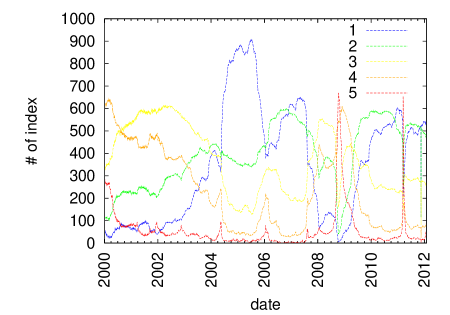
The number of segments belonging to the same quintile of variances is counted. Compute order statistics of variance $\{\sigma_{i,(1)}\leq\ldots\leq\sigma_{i,(m_{i})}\}$ in all the segments of stock $i$. Next, each segment of stock $i$ is labelled $k=\{1,2,3,4,5\}$, depending on variance which belongs to the quintile. The number of segments which have the same labels is counted on each day. Fig. 2 shows the number of segments belonging to each quintile on every day. The number of first quintile segments shows stability of economic affairs, and the number of fifth quintile segments indicates instability of economic affairs. It is found that from 2003 to 2007, the Japanese economy was in a stable regime. From the end of 2007 an unstable regime was observed. Specifically, during September 2008, when we experienced the Lehman shock, the number of fifth quintile regimes steeply increased. This implies that the money flows of the Japanese economy became unstable just after the Lehman shock. From March 2009, the money flow eventually recovered, and the number of unstable regimes decreased while the number of stable segments eventually increased. From 11 March to 10 April, 2011 the number of unstable regimes steeply increased due to the Great East Japan Earthquake. However, the number of stable regimes rapidly increased thereafter, and Japanese macroeconomic affairs have been eventually recovered.

Figure 2: The number of segments in each quintile for 1,413 log-return time series between 4th January 2000 to 30th January 2012.

3.2 Foreign exchange market

The foreign exchange market is the largest financial market in the world. The foreign exchange market is organised by international banks and funds through brokerage platforms. Since the currency exchange strongly reflects and is related to international economies, we can predict global economic conditions from the foreign exchange market.

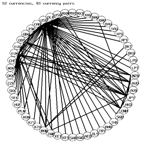
The analysis is conducted using high-resolution data (ICAP EBS Data Mine Level 1.0) collected using the ICAP EBS platform. The data includes currency pairs, quotation prices, and transaction prices with a one-second resolution. In the exchangeable currency pairs, consisting of 41 currencies and 11 precious metals, 93 kinds of currency pairs are included during the period from June 2008 to June 2012. There are about 520 million records in the observation period. Fig. 3 shows exchangeable currency pairs. USD and EUR have a lot of links to other currencies. AUD, CNH, CHF, JPY, and GBP have five to eight links. Others have only one or two links to major currencies.

Figure 3: Network representation of currencies and currency pairs. Nodes represent currencies, and links between two nodes represent currency pairs included in the data set.

Suppose one can observe quotations/transactions about the $i$-th currency, and the $j$-th currency and count the arrival of quotations or occurrence of transactions for each currency pair on a brokerage system with an interval of $\Delta(>0)$. This activity is defined as the number of quotations/transactions which market participants enter into the electronic brokerage system per $\Delta$. We define $f_{ij}(t;S)$ as the quotation activities between the $i$-th currency and $j$-th currency ($i,j=1,2,\ldots,N$) in $[t\Delta,(t+1)\Delta]\quad(t=1,2,\ldots,T)$ on the $S$-th observation period. In this analysis, we adopt the definition that the activities should be counted in symmetrical manner $f_{ij}(t;S)=f_{ij}(t;S)$ and satisfy no self-dealing condition $f_{ii}(t;S)=0$. Then, the density of quotations between the $i$-th currency and $j$-th currency can be estimated as,

$$A_{ij}(S)=\frac{\sum_{t=1}^{T}f_{ij}(t;S)}{\sum_{t=1}^{T}\sum_{i=1}^{N}\sum_{j=1}^{N}f_{ij}(t;S)}.$$ (11)

Obviously, it has probabilistic properties, such that, $\sum_{i=1}^{N}\sum_{j=1}^{N}A_{ij}(S)=1$, $A_{ij}(S)=0$, and $0\leq A_{ij}(S)\leq 1$.

Under the assumption that the attention of market participants to the exchangeable currency pairs can be estimated as the centrality of currency pairs, $A_{ij}(S)$ can be empirically estimated by using quotation/transaction frequencies calculated from high-resolution data without knowledge of the network structure of market participants. Moreover, relative occurrence rates of the $i$-th currency on the $S$-th observation period are defined as,

$$K_{i}(S)=\sum_{j=1}^{N}A_{ij}(S),$$ (12)

where it also has probabilistic properties, such that, $\sum_{i=1}^{N}K_{i}(S)=1$ and $0\leq K_{i}(S)\leq 1$. Since both $A_{ij}(S)$ and $K_{i}(S)$ may be regarded as fingerprints representing the market states on the observation period $S$, their shape may describe market states at $S$. To capture the difference of shapes between $S_{1}$ and $S_{2}$, Jensen-Shannon divergence [33] is employed.

$$D_{cp}(S_{1},S_{2}) = H_{A}\Bigl{(}\bigl{\{}\frac{1}{2}\sum_{k=1}^{2}A_{ij}(S_{k})\bigr{\}}\Bigr{)}-\frac{1}{2}\sum_{k=1}^{2}H_{A}\Bigl{(}\bigl{\{}A_{ij}(S_{k})\bigr{\}}\Bigr{)}$$ (13)

$$D_{c}(S_{1},S_{2}) = H_{K}\Bigl{(}\bigl{\{}\frac{1}{2}\sum_{k=1}^{2}K_{i}(S_{k})\bigr{\}}\Bigr{)}-\frac{1}{2}\sum_{k=1}^{2}H_{A}\Bigl{(}\bigl{\{}K_{i}(S_{k})\bigr{\}}\Bigr{)},$$ (14)

where $H_{A}(A_{ij})$ and $H_{K}(K_{i})$ are, respectively, denoted as the Shannon entropies defined as,

$$H_{A}(\{A_{ij}\}) = -\sum_{i=1}^{N}\sum_{j=1}^{N}A_{ij}\log A_{ij},$$ (15)

$$H_{K}(\{K_{i}\}) = -\sum_{i=1}^{N}K_{i}\log K_{i}.$$ (16)

From these definitions, we can confirm that they have the following properties:

$$D_{cp}(S_{1},S_{2}) = D_{cp}(S_{2},S_{1}),$$ (17)

$$D_{cp}(S_{1},S_{2}) \geq 0,$$ (18)

$$D_{cp}(S_{1},S_{2}) = 0\quad\mbox{iff}\quad A_{ij}(S_{1})=A_{ij}(S_{2})\forall{i,j},$$ (19)

$$D_{c}(S_{1},S_{2}) = D_{c}(S_{2},S_{1}),$$ (20)

$$D_{c}(S_{1},S_{2}) \geq 0,$$ (21)

$$D_{c}(S_{1},S_{2}) = 0\quad\mbox{iff}\quad K_{i}(S_{1})=K_{i}(S_{2})\forall{i}.$$ (22)

The similarity of market states between two observation periods is computed for each week. The Jensen-Shannon divergence is employed in order to compute similarities since it has resistance characteristic for zero probabilities. This means that the Shannon entropy does not diverge to infinity because of $0\log 0=0$, which is proven in A.

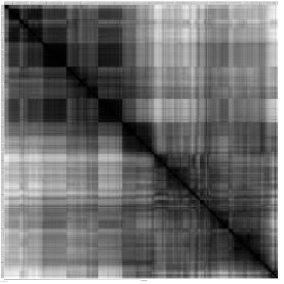
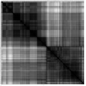
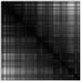
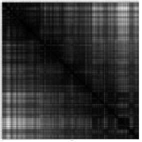
Figs. 4 and 5 show similarities calculated from $A_{ij}(S)$ of quotations (a), $K_{i}(S)$ of quotations (b) and similarities obtained from $A_{ij}(S)$ of transactions (a), and $K_{i}(S)$ of transactions (b), respectively.

(a) (b)

Figure 4: The similarities of market states between observation periods computed from activities of currency pairs (a) and of currencies (b) computed from quotations for the period from June 2007 to June 2012. The black pixel represents a similar relation, and the white pixel represents a dissimilar relation.

(a) (b)

Figure 5: The similarities of market states between observation periods computed from activities of currency pairs (a) and of currencies (b) computed from transactions for the period from June 2007 to June 2012. The black pixel represents a similar relation, and the white pixel represents a dissimilar relation.

From these figures, there are regimes where shares are equivalent. Macroeconomic situations may correspond to these regimes. For example, there are three regimes for the period from January 2008 to June 2009 as shown in Fig. 4. These regimes are related to the last global financial crisis. Furthermore, we can confirm the Euro shock which happened March to May 2010. We can capture both the past and present circumstances of the international economy from the high-resolution data, and may predict or infer the future affair. It is also found that there is an extreme regime in 14 to 21 March, 2011. This event was observed with the sudden increase of JPY in relation to other currencies (specifically USD and EUR). This chaos was triggered by the devastation caused by the Great East Earthquake of Japan and the subsequent tsunami.

3.3 Domestic hotel booking data

Recent technological developments enable us to purchase various kinds of items and services via e-commerce systems. The emergence of Internet applications has had an unprecedented impact on our ability to purchase goods and services. From the data available about items and services on e-commerce platforms, we may expect that utilities of agents in socio-economic systems are directly estimated.

It is found that it is becoming more popular to make reservations of hotels via the Internet. When we use a hotel booking site, we notice that we sometimes find preferable room opportunities. In other words, hotel vacancies seem to be random. We further know that both the date and place of stay are important factors to determine the availability of room opportunities. Hence, room availability depends on the calendar (weekdays, weekends, and holidays) and regions.

This availability of hotel rooms may indicate future migration trends of travellers. Therefore, it is worth considering the accumulation of comprehensive data of hotel availability in order to detect inter-migration within countries.

Here, we give a brief explanation of a method for collecting data on hotel availability. In this study, we used a web API in order to collect the data from a Japanese hotel booking site named Jalan. The data is provided by the Jalan web service [34]. Jalan is one of the most popular hotel reservation services in Japan. The API is an interface code set designed for the purpose of simplifying the development of application programs.

The Jalan web service provides interfaces for both hotel managers and customers. The mechanism of Jalan is as follows: Hotel managers can enter information on room vacancies at their hotels via an web interface. The consumers can book rooms from available opportunities via the Jalan web site. Third parties can even built their web services with Jalan data by using the web API.

We collected all available opportunities which appeared on Jalan web regarding one-night room vacancies for two adults. The data were sampled from the Jalan web service daily. The data on room opportunities collected through the Jalan web API are stored as comma separated value (csv) files.

In the data set, there exist over 100,000 room opportunities at over 14,000 hotels. In Table 1, we show contents included in the data set. Each plan contains sampled date, stay date, regional sequential number, hotel identification number, hotel name, postal address, URL of the hotel website, geographical position, plan name, and rate.

Since the data contains regional information, it is possible for us to analyse regional dependence of hotel rates. Throughout the investigation, we regard the number of recorded opportunities (plan) as a proxy variable of the number of available room stocks.

Table 1: The data format of room opportunities.

Date of collection

Date of stay

Hotel identification number

Hotel name

Hotel name (kana characters)

Postal code

Address

URL

Latitude

Longitude

Opportunity name

Meal availability

The latest best rate

Rate per night

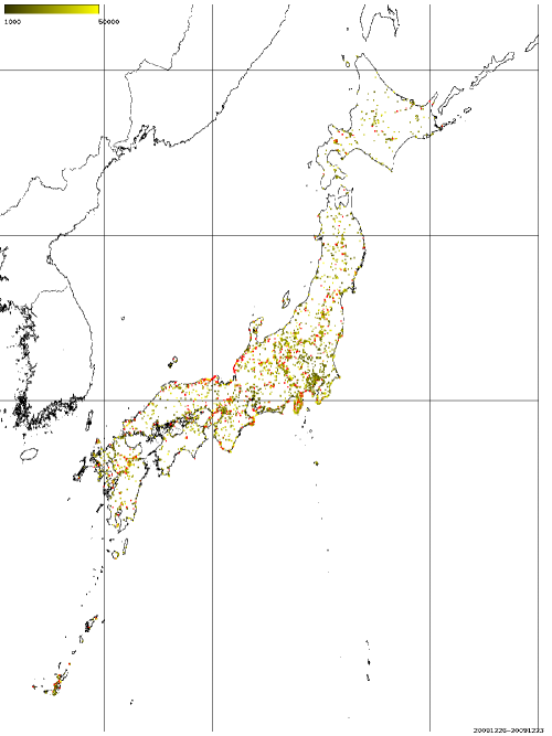
For this analysis, we used the data for the period from 24 December, 2009 to 8 May, 2011. The data is missing from 14 to 30 March, 2011 because the the web service was not available due to the Great East Earthquake. Fig. 6 shows an example of distributions and representative rates. An example of rates distributions under the condition that two adults can stay at the hotel for one night at 23 December, 2009. This data have been sampled on 25 December, 2009. The yellow to red filled squares represent hotel plans costing ranging from 50,000 to JPY 1,000 JPY per night. The red filled squares represent hotel plans costing over 50,000 JPY per night. We found that there was a strong dependence of vacancies on places. Specifically, we find that many hotels are located around several centralised cities such as Tokyo, Osaka, Nagoya, Fukuoka, and so on.

Figure 6: The regional dependence of room prices of Japanese available on 26 December, 2009, as of 23 December, 2009.

Figure 7: The number of room plans for one-night stay by two adults during the period between 24 December, 2009 to 8 May, 2011.

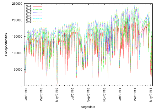
The number of one-night, twin-share room plans was counted from the recorded csv files throughout the whole sampled period. Fig. 7 shows the daily number of room opportunities with different durations $D$, which is defined as a difference between stay date and booking date. From this graph, we found three facts:

(1) The number of room opportunities fluctuates weekly.

(2) There is a strong dependence of the number of available opportunities on the Japanese calendar. Namely, Saturdays and holidays drove reservation activities of consumers. For example, during the New Year holidays (around 12/30-1/1) and holidays in the spring season (around 3/20), the time series of the numbers show big drops.

(3) The number eventually increases as the date of stay reaches. Specifically, it is observed that the number of opportunities drastically decreases two days before the date of stay.

Figure 8: Average prices for one-night, twin-share room plans throughout Japan for the period from 24 December, 2009 to 8 May, 2011.

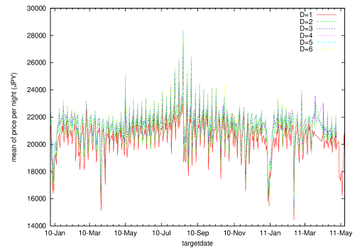
Furthermore, Fig. 8 shows dependence of average rates all over the Japan on calendar dates with different durations. During the New Year holidays in 2010, the average rates rapidly decreased. Meanwhile, on the spring holidays in 2010, the average rates rapidly increased. This difference seems to arise from the difference of consumers’ motivation structure and preference on price levels between these holiday seasons.

Figure 9 shows scatter plots between the daily number of room opportunities and average of room rates. The high-demand dates exhibit larger variations of the average rate than low-demand dates. The preferable price level of consumers has a high variability on high-demand dates.

Figure 9: Scatter plots between the daily number of room opportunities and mean room rates across Japan for the period from 24 December, 2009 to 10 June, 2011.

3.4 Impact of natural disasters (Great East Japan Earthquake on 11 March, 2011)

Since people are also products of nature, the physical effects of the natural environment on our society are remarkable. Specifically, natural disasters often affect our societies significantly. Therefore, we need to understand the subsequent impact of natural disasters on human behaviour, from both economical and social perspectives.

The first Great East Japan Earthquake hit at 14:46 on 11 March, 2011 in Japanese local time (05:46 in UTC). Within 20 minutes, huge tsunamis had devastated cities along Japan’s northeastern coastline. In addition to wide-spread physical destruction, social infrastructures also suffered extensive damaged. It is important for us to understand its subsequent impact on our socio-economic activities.

In order to estimate both economic and social damages in three Tohoku prefectures (Iwate, Miyagi, and Fukushima), we focus on the number of available hotels in each district before and after the Great East Japan Earthquakes and Tsunami. We selected 21 districts in three prefectures, as shown in Table I and two periods, one before and one after the disaster. The data on accommodation in this area cover about 31% of the potential accommodation. Therefore, we have to estimate the states that were not sampled from these sampled booking data.

If we assume that the accommodations in the data are sampled from uncensored data in a homogeneous way, then the relative frequency of the available accommodation from censored data can approximate the true value, computed from uncensored data. The data on accommodations in this area cover about 31% of the potential accommodation. Therefore, we have to estimate the uncensored states from these censored booking data.

If we assume that accommodation in the data are sampled from uncensored data in a homogeneous way, then a relative frequency of the available accommodations from censored data can approximate the true value that would be computed from uncensored data.

In order to conduct a qualitative study, let $x_{i}(t,s)\quad(i=1,\ldots,K;t=1,\ldots,T)$ be the number of available hotels in district $i$ at day $t$ in period $s$. Then a relative frequency at district $i$ can be calculated as,

$$p_{i}(s)=\frac{\sum_{t=1}^{T}x_{i}(t,s)}{\sum_{i=1}^{K}\sum_{t=1}^{T}x_{i}(t,s)}.$$ (23)

Let us consider a ratio of the relative frequencies after and before a specific event,

$$q_{i}(a|b)=p_{i}(a)/p_{i}(b),$$ (24)

where $p_{i}(a)$ and $p_{i}(b)$ represent the relative frequencies after and before the event, respectively. Obviously, Eq. 24 can be rewritten as:

$$q_{i}(a|b)=\frac{n_{i}(a)}{n_{i}(b)}/\frac{N(a)}{N(b)},$$ (25)

by using $n_{i}(s)$ and $N(s)$, which are the number of available hotels at district $i$ within the period $s$ and the total number during that period. Since $N(a)/N(b)$ is independent of $i$, $q_{i}(a|b)$ should be proportional to a ratio of the number of hotels after and before the event.

Table 2 shows $q_{i}(a|b)$, where the term $b$ represents May 2010 (before the disaster), and the term $a$ May 2011 (after the disaster), respectively. Since the value of $q_{i}(a|b)$ is related to damage to hotels in the district $i$, $q_{i}(a|b)<1$ implies that available hotels decreased after the earthquake at $i$ relative to the total number of hotels. Similarly $q_{i}(a|b)>1$ means that they maintained at $i$.

We may assume that the decrease of $q_{i}(a|b)$ at district $i$ results from both a decrease of supply and an increase of demand. The decrease of supply is caused in this case by the physical destructions of infrastructure. The increase of demand comes from behaviour of individuals like refugees, workers, volunteers, and civic groups.

The regional dependence of supply can be estimated from the number of destroyed houses in each district. To do so, we calculate the numbers of both completely-destroyed and partially-destroyed houses at each district from the data downloaded from a website of the National Research Institute for Earth Science and Disaster Prevention [35]. The numbers are calculated by summing the number of destroyed houses in the towns or cities included in each district. Table 2 shows the numbers of destroyed houses. In this histogram it is shown that damaged houses were concentrated in the maritime areas of these prefectures.

Table 2: The ratio of the number of available hotels during the period from 1st to 31st May 2011 to that during the period from 1st to 31st May 2010 (after and before the Great East Japan Earthquake), the number of both completely destroyed houses and partially destroyed houses, as confirmed at the end of September 2011 and the number of evacuees, as confirmed at 1st May 2011.

prefecture	district	ratio	complete collapse	partial collapse	evacuees
Iwate	Shizukuishi	1.970	0	0	372
	Morioka	1.834	0	4	366
	Appi,Hachimantai,Ninohe	2.250	3	0	0
	Hanamaki,Kitakami,Tohno	1.350	27	364	853
	SanrikuKaigan	0.481	18,098	2,166	12,896
	Oushu,Hiraizumi,Ichinoseki	0.374	83	533	338
Miyagi	Sendai	0.550	21,789	37,522	3,608
	Matsushima,Shiogama	0.345	7,895	12,581	5,115
	Ishinomaki,Kesennuma	0.0	33,661	6,083	23,840
	Naruko,Osaki	1.484	486	1,577	929
	Kurihara,Tome	1.404	224	1,105	1,049
	Shiroishi,Zao	1.608	2,522	1,644	1,612
Fukushima	Fukushima,Nihonmatsu	0.665	168	1,898	1,321
	Soma	0.038	6,279	1,618	1,969
	Urabandai,BandaiKogen	1.134	0	0	2
	Inawashiro,Omotebandai	1.009	10	12	303
	Aizu	1.352	4	27	266
	Minamiaizu	1.768	0	0	14
	Koriyama	0.604	2,596	12,185	2,489
	Shirakawa	1.915	135	1,820	418
	Iwaki,Futaba	0.195	6,550	17,614	2,115

Table 3: The number of evacuees of the Great East Japan Earthquake at three prefectures (Iwate, Miyagi, and Fukushima). The data were officially announced by the Japanese Cabinet Office on 3rd June 2011.

prefecture	A: public places	B: hotels	C: others	A+B+C
Aomori	0	78	777	855
Iwate	9,039	2,007	14,701	25,747
Miyagi	23,454	2,035	-	25,489
Akita	128	619	909	1,656
Yamagata	305	779	2,366	3,450
Fukushima	6,105	17,874	-	23,979

We can confirm that house damage was serious in Sanrikukaigan, Sendai, Matsushima, Shiogama, Ishinomaki, Kesennuma, Soma, Koriyama, Iwaki, and Futaba. The greatest number of completely-destroyed houses is 33,661 in Ishinomaki and Kesennuma. The second is 21,789 in Sendai. The third is 18,098 in Sanrikukaigan. The greatest number of partially-destroyed houses is 37,522 in Sendai. The second is 17,614 in Iwaki and Futaba. The third is 12,185 in Koriyama.

In fact, in places where the ratio $q_{i}(a|b)$ is greater than 1, the number of destroyed houses is not significant, as shown in Figure 2. We confirmed that the ratio $q_{i}(a|b)$ may measure the degree of damage to economic activity in the travel industry. However, it is not confirmed that there was significant physical damage to houses in Oushu, Hiraizumi, Ichinoseki, Fukushima, and Nihonmatsu, even having a ratio less than 1. It may be thought that hotels in Oushu, Hiraizumi, and Ichinoseki were used by workers and evacuated victims of the disaster. Decreases of available hotels in Fukushima and Nihonmatsu may be related to accidents in Fukushima Daiich nuclear power plant. The number of victims evacuated from the disaster in each prefecture, according to an official announcement by the Japanese Cabinet Office on 3 June 2011, is shown in Table 3. In the case of Fukushima prefecture, 17,874 people were evacuated to hotels at that time.

3.5 International flight booking data

AB-ROAD [36] is a Japanese Internet travel booking site. About 14,000 flights are available on this site every day. This booking site serves as a web API for both travel agencies and customers. On the one hand, travel agencies can register their flight opportunities on the site via the Internet. On the other hand, consumers can search for and book flights that they want to purchase from all the registered flights via the website. Third parties can even build web services with the data provided by the web API.

I collected information regarding available flight tickets using the AB-ROAD web service every day and stored it as comma-separated (CSV) files. This data set contains the flight tickets that a person would be able to use to depart from one of the airports in Japan. Each flight also contains the date when the data was sampled, departure date, departure airport, arrival airport, type of class (economy, business, and first), name of air carrier, and price (the fuel surcharge and tax are excluded). The data period is from 29 July, 2010 to 14 December, 2011. For technical reasons, data on several dates is missing (8 November, 2010, 10 April, 2011, from 14 to 25 April, 2011).

We use data of opportunities where flights would depart from some airports in Japan 4 weeks later. The supply-demand situation of air travels may be related to the number of opportunities. The price of flight tickets between departure and arrival airports is also dependent on their distance. Fundamentally, I investigates current situations of international air flights departing from Japanese airports. In the dataset, there exist about 14,000 kinds of flight opportunities for about 78 airline companies  every day.

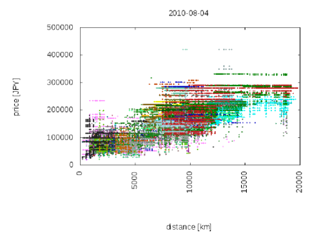
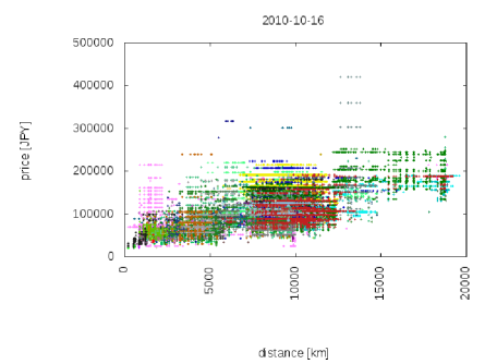
The total number of available flights from a city in Japan to a city in a foreign country was totalled from the data throughout the entire sampled period. Figure 10 shows the total number of available flights per day. From observing this data, we made three observations:

(1) There exists weekly seasonality for the total number of available flight tickets. The demand of flight tickets is higher on Sundays and Mondays than on other days.

(2) The number of flight tickets strongly depends on the Japanese calendar. Namely, summer holidays influence the reservation activities of consumers. For example, during the Golden Week holidays (from 1 to 5 May, 2011) and the holidays in the spring season (around 20 March, 2011), total availability shows steep decreases.

(3) Since several airline companies update their flight schedule every April and October, ticket availability drastically drops at that time.

Figure 10: The daily number of flight opportunities from 29 July, 2010 to 24 December, 2011.

Recently, the airport network has been studied by several researchers [37, 38, 39]. According to the study by Guimerà and Amaral [37], the world-wide airport network has properties of a small-world network. The degree and betweenness centrality distributions exhibit power-law decay. In fact, the most connected cities (largest degree) are typically not the most central cities (largest betweenness centrality). Airports with high betweenness tend to play a more important role in keeping networks connected than those with high degree, because a passenger can travel from a departure airport to a destination with a short path. The geodesic distance between departure and arrival airports may give a good approximation of the actual flight distance of passengers.

The geodesic distance is measured by Vincenty’s formulae. Let $\phi_{s}$, $\lambda_{s}$, $\phi_{f}$ and $\lambda_{f}$ be the geographical latitude and longitude of two points, respectively, and $\Delta\lambda=\lambda_{s}-\lambda_{f}$. Under the assumption that the earth is a sphere, the distance $D$ is given by,

$$D=r\tan^{-1}\Bigl{(}\frac{\sqrt{(\cos\phi_{s}\sin\Delta\lambda)^{2}+(\cos\phi_{s}\sin\phi_{f}-\sin\phi_{s}\cos\phi_{f}\cos\Delta\lambda)^{2}}}{\sin\phi_{s}\sin\phi_{f}+\cos\phi_{s}\cos\phi_{f}\cos\Delta\lambda}\Bigr{)},$$ (26)

where $r$ represents the earth’s radius ($r=6371.2$ [km]). It is possible to analyse the geodesic dependence of ticket prices with this data. Figure 11 shows the relation between the price of economy-class flight tickets and the geodesic distance from the departure airport to the destination. The distance of each flight ticket is computed from the geographical latitude and longitude of the departure and arrival airports using Equation (1). Fig. 11 represents the relationship on 4 August, 2010 (high demand season) and on 16 October, 2010 (low demand season). Short-distance corresponds to flights to Asian cities (1,000 km to 3,000 km), middle-distance to cities in Europe and North America (8,000 km to 10,000 km), and long-distance to cities in South America (15,000 km to 20,000 km). During high demand season, it is found that various kinds of flights appear for both short-distance and long-distance flights, but, during low demand season, there are few long-distance flights.

(a) (b)

Figure 11: Relationship between the price of economy-class flights and geodesic distance on 4 August, 2010 (a) and on 16 October, 2010 (b).

4 Discussion

It was shown from looking at these exemplar studies that there are two kinds of axes with which to best represent our society. The studies of the Japanese stock exchange market and the foreign exchange market show that different stocks or currencies are quoted or traded concurrently, and that they are mutually related. Namely, time is one of important key factors to link data observed in different places. Investigation of both the hotel and international flights showed that geographical information is also a key factor to link data from different layers.

Since events in the world happen in massively concurrent, time and locations are the most important elements to link results obtained from different data sources. Furthermore, we may synthesise data from different data sources with a time and location, and construct a large-scale database.

I also want to say that these studies are of econoinformatics. Econoinformatics includes several research topics such as mathematical concepts, algorithms, computer systems, databases, modelling, and so forth. Mathematical concepts may help us to develop automated algorithms to extract knowledge on socio-economic systems. The algorithm and computation systems help us to collect, store and analyse large amounts of data. It is also crucial to construct synthesised data sets from uncensored data obtained from different data sources. Furthermore, mathematical models will become a guide for us to understand observed systems connecting physical mechanisms with observations.

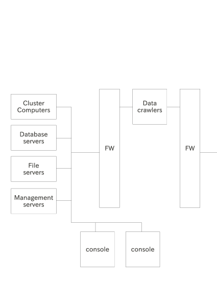
Figure 12 shows a conceptual illustration of a research platform. This consists of data crawlers, cluster computers, database servers, management servers, file servers, and consoles. The data crawlers collect socio-economic data from e-commerce platforms in the internet. The data is stored in the file servers. After verifying the data, the data is synthesised in the database servers. To construct the synthesised database, the data is stored with the time and/or locations. The management servers handle this procedure of collecting, verifying, and storing data automatically. In the cluster computers, the socio-economic data is computed and analysed. Researchers use this system from the consoles.

Figure 12: A conceptual illustration of the research platform.

5 Conclusion

The concept of complexity was discussed from several points of view. Complexity is determined by the relative degrees of freedoms of observing systems and of observed systems. Recent exemplar studies on data-centric socio-economic systems were reviewed and presented. The Japanese stock exchange, foreign exchange market, domestic hotel bookings, and international flight bookings were analysed from a comprehensive point of view.

Econoinformatics can be established from data-centric studies based on large amounts of data on socio-economic systems. Such data can be obtained from our society. To overcome the complexity of socio-economic data, we need to develop mathematical concepts, algorithms, rich computer systems, and synthesised databases. To construct synthesised data on socio-economic systems, spatial-temporal axes should be employed. Various kinds of data collected from different paths may be synthesised with time and locations. Rich synthesised databases representing aspects of our society may help us to obtain deeper insights into our own socio-economic systems.

References

Appendix A Proof of $0\log 0$

Let us consider

$$h=\lim_{x\rightarrow+0}x\log x.$$ (27)

Putting $x=e^{-z}$ one has

$$h=-\lim_{x\rightarrow+0}ze^{-z}.$$ (28)

By using the Taylor expansion of $e^{z}=\sum_{k=0}^{\infty}\frac{1}{k!}z^{k}$, one obtains

$$h = -\lim_{z\rightarrow\infty}ze^{-z}$$ (29)

$$= -\lim_{z\rightarrow\infty}z/e^{z}$$

$$= -\lim_{z\rightarrow\infty}\frac{z}{\sum_{k=0}\frac{1}{k!}z^{k}}$$

$$= -\lim_{z\rightarrow\infty}\frac{1}{\sum_{k=0}\frac{1}{k!}z^{k+1}}$$

$$= 0.$$

Therefore, we gets

$$h=\lim_{x\rightarrow 0}x\log x=0\log 0=0.$$ (30)

References

- [1] Goodchild M F 2007 Citizens as voluntary sensors: spatial data infrastructure in the world of Web 2.0 International Journal of Spatial Data Infrastructures Research 2 24
- [2] EU FP-8 FET Flagship: FuturICT http://www.futurict.eu
- [3] Dehmer M and Mowshowitz A 2011 A history of graph entropy measures Information Sciences 181 57
- [4] Wilhelm T and Hollunder J 2007 Information theoretic description of networks Physica A 385 385
- [5] Rashevsky N 1955 Life, information theory, and topology Bull. Math. Biophys. 17 229
- [6] Trucco E 1956 A note on the information content of graphs Bull. Math. Biophys. 18 129
- [7] Mowshowitz A 1968 Entropy and the complexity of graphs: I. An index of the relative complexity of a graph Bull. Math. Biophys. 30 175
- [8] Sato A H 2010 Comprehensive analysis of information transmission among agents: similarity and heterogeneity of collective behaviour Agent-based in Economic and Social Systems VI: Post-Proceedings of The AESCS International Workshop 2009, Agent-Based Social Systems 8 ed S.-H. Chen et al. (Tokyo: Springer) pp 1–17.
- [9] Bianconi G 2009 Entropy of network ensembles Phys. Rev. E 79 036114
- [10] Anand K and Bianconi G 2009 Entropy measures for networks: Toward an information theory of complex topologies Phys. Rev. E 80 045102
- [11] Foerster v H 1984 Observing Systems (California: Intersystems Publications)
- [12] von Neumann J 1958 The Computer and the Brain (New Haven/London: Yale Univesity Press)
- [13] Landauer T K 1986 How much do people remember? Some estimates of the quantity of learned information in long-term memory Cognitive science 10 477
- [14] New IT Infrastructure for the Information-explosion Era (July 2005–March 2011) URL: http://www.infoplosion.nii.ac.jp/info-plosion/ctr.php/m/IndexEng/a/Index/
- [15] Korth H F 1997 Database research faces the information explosion Communications of the ACM 40 139
- [16] Takayasu H 2002 The Advent of Econophysics (Tokyo: Springer)
- [17] Mantegna R N and Stanley H E 2000 An Introduction to Econophysics: Correlations and Complexity in Finance (Cambridge: Cambridge University Press)
- [18] Sornette D 2003 Why Stock Markets Crash: Critical Events in Complex Financial Systems (Princeton: Princeton University Press)
- [19] Sato A H and Hołyst J A 2008 Characteristic periodicities of collective behavior at the foreign exchange market Eur. Phys. J. B 62 373
- [20] Portal Site of Official Statistics of Japan by National Statistics Center: http://www.e-stat.go.jp
- [21] González M C, Hidalgo C A and Barabási A L 2008 Understanding individual human mobility patterns Nature 453 479
- [22] Antoniou C, Ben-Akiva M and Koutsopoulos H N 2006 Dynamic traffic demand prediction using conventional and emerging data sources IEE Proc. Intell. Transp. Syst. 153 97
- [23] ed Helbing D 2007 Managing Complexity: Insights, Concepts, Applications (Berlin: Springer)
- [24] Mizuno T, Toriyama M, Terano T and Takayasu M 2008 Pareto law of the expenditure of a person in convenience stores Physica A 387 3931
- [25] Lambiotte R and Ausloos M 2005 Endo-vs. exogenous shocks and relaxation rates in book and music sales Physica A 362 485
- [26] Deschâtres F and Sornette D 2005 Dynamics of book sales: Endogenous versus exogenous shocks in complex networks Phys. Rev. E 72 016112
- [27] Sato A H 2012 Patterns of regional travel behavior: an analysis of Japanese hotel reservation data Int. Rev. of Finan. Anal. 23 55
- [28] Sato A H 2012 Japanese international air travel: the relationship between flight ticket price and geodesic distance Proc. 2012 IEEE World Congress on Computational Intelligence (Brisbane) pp 2821-2826
- [29] Mizuno T and Watanabe T 2010 A statistical analysis of product prices in online market Eur. Phys. J. B 76 501
- [30] Goldfeld S M and Quandt R E 1973 A Markov model for switching regressions J. Econometrics 1 3
- [31] Cheong S A, Fornia R P, Lee G H T, Kok J L, Yim W S, Xu D Y and Zhang Y 2012 The Japanese economy in crises –A time series segmentation study Economics E-journal 6 2012-5, www.economics-ejournal.org
- [32] Bernaola-Galván P, Román-Roldán R and Oliver J L 1996 Compositional segmentation and long-range fractal correlations in DNA sequences Phys. Rev. E 53 5181
- [33] Lin J 1991 Divergence measures base on the Shannon entropy IEEE Trans. on Info. Theor. 37 145
- [34] The data is downloaded from Jalan Web service: http://www.jalan.net
- [35] The data is downloaded from a Web page of National Research Institute for Earth Science and Disaster Prevention: http://www.j-risq.bosai.go.jp/ndis/ (31 Aug 2011).
- [36] The data is downloaded from AB-ROAD Web service: http://www.ab-road.net
- [37] Guimerà R and Amaral L A N 2004 Modeling the world-wide airport network Eur. Phys. J. B 38 381
- [38] Guida M and Maria F 2007 Topology of the Italian airport network: A scale-free small-world network with a fractal structure? Chaos, Solitons and Fractals 31 527
- [39] Bagler G 2008 Analysis of the airport network of India as a complex weighted network Physica A 387 2972
Appendix A Proof of