Spectral Energy Distributions of low-luminosity radio galaxies at z$\sim 1-3$:
a high-zview of the host/AGN connection.

Abstract

We study the Spectral Energy Distributions, SEDs, (from FUV to MIR bands) of the first sizeable sample of 34 low-luminosity radio galaxies at high redshifts, selected in the COSMOS field. To model the SEDs we use two different template-fitting techniques: i) the Hyperz code that only considers single stellar templates and ii) our own developed technique 2SPD that also includes the contribution from a young stellar population and dust emission. The resulting photometric redshifts range from z$\sim$0.7 to 3 and are in substantial agreement with measurements from earlier work, but significantly more accurate. The SED of most objects is consistent with a dominant contribution from an old stellar population with an age $\sim 1-3\times$ 10⁹ years. The inferred total stellar mass range is $\sim$10${}^{10}-10^{12}$ M_⊙. Dust emission is needed to account for the 24 $\mu m$ emission in 15 objects. Estimates of the dust luminosity yield values in the range $L_{\rm dust}\sim 10^{43.5}-10^{45.5}$ erg s^-1. The global dust temperature, crudely estimated for the sources with a MIR excess, is $\sim$ 300-850 K. A UV excess is often observed with a luminosity in the range $\sim 10^{42}-10^{44}$ erg s^-1 at 2000 Å  rest frame.

Our results show that the hosts of these high-z low-luminosity radio sources are old massive galaxies, similarly to the local FRIs. However, the UV and MIR excesses indicate the possible significant contribution from star formation and/or nuclear activity in such bands, not seen in low-z FRIs. Our sources display a wide variety of properties: from possible quasars at the highest luminosities, to low-luminosity old galaxies.

1. Introduction

The search for radio-loud Active Galactic Nuclei (AGN) is one of the widely used tools to study the distant universe (z $>$ 1). Indeed the first objects found at z $>$ 1 were radio-loud quasars (see Stern & Spinrad 1999 and references therein) and a large number of radio galaxies ($\sim$300) are known to exist at high redshifts (e.g., Miley & De Breuck 2008).

Flux-limited samples of radio galaxies such as the 3CR and its deeper successors 6C and 7C catalogs are affected by a tight redshift-luminosity correlation. This, alongside with the steep luminosity function of radio sources, gives rise to a selection bias which results in the presence of high power sources predominantly at high redshifts only and low power sources exclusively at low redshift. Therefore, our knowledge of radio galaxies and their hosts at high redshifts is exclusively based on studies of powerful (edge-brightened, Fanaroff & Riley 1974) FR IIs. Thus, the properties of the low-luminosity AGN population in the early Universe is essentially unknown. The missing pieces of the puzzle might be obtained by studying a sample of low luminosity (’edge-darkened’, Fanaroff & Riley 1974) FR Is at high redshifts. The lower power of these objects with respect to that of high-z FR IIs might allow us to analyze with more clarity the properties of the hosts at high redshifts. Furthermore, in terms of host galaxy properties, low power sources are both more abundant and most likely more similar to quiescent galaxies (in terms of host galaxy properties) than FR IIs.

Only a few FR Is at high redshift are present in the 7C sample (Heywood et al., 2007) and two were possibly found in HDF North (Snellen & Best, 2001). Chiaberge et al. (2009) obtained the first sizeable sample of 37 FR I candidates at z $\gtrsim 1$, located in the 2 deg² area of the sky observed by the COSMOS survey (Scoville et al., 2007). In this paper we perform a detailed analysis of the photometric properties of the host galaxies of these radio sources, by taking advantage of the large multi-wavelength coverage provided by the COSMOS collaboration. This allows us to derive their spectral energy distributions (SEDs) from $\sim$ 0.15 $\mu$m to 24 $\mu$m. We then model the obtained SEDs with synthetic stellar population templates with the aim of both inferring the properties of each galaxy and of deriving an accurate estimate of the photometric redshifts.

Mobasher et al. (2007) and Ilbert et al. (2009) performed a similar study with the aim of determining the photo-z for the whole COSMOS sample. However, as already noted by Chiaberge et al. (2009), the faint counterparts of these radiogalaxies might be easily misidentified or be missed from the COSMOS catalog. Therefore a careful object-by-object study of the sample is necessary to correctly identify the genuine counterparts of the radio sources at all wavelengths. This allows us to obtain reliable SEDs and perform a robust study of the hosts of these objects. In this work, using the multi-band data provided by the COSMOS survey (described in Section 3), we obtain the photometric data from the catalog checking visually the correct identification of each object of the sample (Section 4). In Section 5 we describe the codes used to model the SEDs, Hyperz and 2SPD. We present the results obtained from the SED modeling in Section 6: the photometric redshifts, the radio power distribution, and the host properties, such as stellar ages, masses and dust and UV components. In Section 7 we summarize the results and we discuss our preliminary findings.

We adopt a Hubble constant of H₀ = 71 km s^-1 Mpc^-1, $\Omega_{m}$ = 0.27 and $\Omega_{vac}$ = 0.73, as given by the WMAP cosmology (e.g., Spergel et al. 2003; Jarosik et al. 2011). All the magnitudes are in AB mag system, if not otherwise specified.

2. Sample

Chiaberge et al. (2009) selected a sample of 37 high-z low-power radio galaxies at z $\sim$ 1-2 in the Cosmic Evolution Survey (COSMOS) field (Scoville et al., 2007). This is the first sizeable sample of low-power radio sources at mid- to high-redshifts. This sample has been obtained with a four-steps multi-wavelength selection process, which is described in detail in Chiaberge et al. (2009). Here we briefly summarize the selection procedure which depends on the following assumptions: i) the FR I/FR II break luminosity at 1.4 GHz does not change with redshift, and ii) the host properties of distant low-luminosity sources are similar to those of high-power FR IIs in the same redshift range.

The first step consists of selecting radio sources from the FIRST catalog (Becker et al., 1995) whose 1.4 GHz total flux corresponds to the luminosities expected by FR Is at 1$<z<$2. The second step is based on a radio morphological classification: the radio sources which show clear “edge-brightened” structures are rejected in order to exclude the bona-fide FR IIs from the sample. The third step implies the optical identification of the radio sources in the COSMOS optical images. The objects associated with host galaxies brighter than $i$ $<$ 22 were rejected to exclude lower redshifts starburst galaxies. As a final step, u-band dropouts are also rejected since these are objects most likely located at redshift higher than z=2. The resulting sample consists of 37 FR I candidates. A posteriori, the photometric redshifts range of most of them is between $\sim$1 and $\sim$2 (Mobasher et al., 2007; Ilbert et al., 2009), with the exception of 3 objects (namely, 7, 27, and 66) that we exclude from any further analysis because out of the redshift range of interest. We are then left with a final sample of 34 objects. The list of the radio sources is presented in Table 1.

Table 1Radio positions, redshifts and radio flux of the sample

ID	RA	DEC	zphot,Ilbert	zspec	FNVSS	FFIRST
1	150.20744	2.2818749	0.92${}^{+0.02}_{-0.06}$	0.8827a-0.8823b	$<$2.5	1.79
2	150.46751	2.7598829			2.6	1.08
3	150.00253	2.2586310	1.96${}^{+0.36}_{-0.41}$		5.2	4.21
4	149.99153	2.3027799	1.45${}^{+0.08}_{-0.15}$		7.5	5.99
5	150.10612	2.0144780	1.84${}^{+0.22}_{-0.12}$		3.4	1.30
11	150.07816	1.8985500	1.31${}^{+0.60}_{-0.24}$		$<$2.5	1.13
13	149.97784	2.5042069	1.09${}^{+0.06}_{-0.06}$		2.4	1.51
16	150.53772	2.2673550	0.95${}^{+0.05}_{-0.02}$	0.9687b	4.4	5.70
18	149.69325	2.2674670	0.92${}^{+0.01}_{-0.09}$		5.1	4.39
20	149.83209	2.5695460	1.00${}^{+0.02}_{-0.05}$		$<$2.5	1.33
22	149.89508	2.6292144			$<$2.5	2.74
25	150.45673	2.5597000	1.12${}^{+0.29}_{-0.03}$	0.7917b∗	2.7	2.18
26	149.62114	2.0919881	1.20${}^{+0.06}_{-0.02}$		3.2	1.88
28	149.60064	2.0918673			2.4	1.77
29	149.64587	1.9529760	1.59${}^{+0.45}_{-0.30}$		2.3	2.12
30	149.61542	1.9910541	0.90${}^{+0.31}_{-0.03}$		2.4	1.26
31	149.61916	1.9163600	0.91${}^{+0.02}_{-0.05}$	0.9132a-0.9123b	4.1	3.71
32	149.66830	1.8379777			3.1	1.31
34	150.56023	2.5861051	1.42${}^{+0.65}_{-0.32}$		4.5	5.25
36	150.55662	1.7913361			3.3	3.19
37	150.74336	2.1705379	1.27${}^{+0.09}_{-0.02}$		2.2	1.87
38	150.53645	2.6842549	1.12${}^{+0.10}_{-0.05}$		11.6	10.01
39	149.95804	2.8288901	1.08${}^{+0.03}_{-0.03}$		$<$2.5	1.37
52	149.90590	2.3964710	0.74${}^{+0.02}_{-0.03}$	0.7417b	$<$2.5	1.54
70	150.61987	2.2894360	2.21${}^{+0.57}_{-0.37}$		4.5	3.90
202	149.99506	1.6324950	1.19${}^{+0.24}_{-0.14}$		3.3	1.08
219	150.06444	2.8754051	1.04${}^{+0.01}_{-0.09}$		$<$2.5	1.85
224	150.28999	1.5408180	1.10${}^{+0.07}_{-0.03}$		3.2	3.31
226	150.43864	1.5934480	1.76${}^{+0.61}_{-0.14}$		$<$2.5	1.19
228	149.49455	2.5052481	1.89${}^{+0.74}_{-0.59}$		3.7	2.04
234	150.78925	2.4539680	1.10${}^{+0.12}_{-0.03}$		5.2	4.43
236	150.70554	2.6296339		2.132c	7.0	7.10
258	149.55934	1.6310670	0.90${}^{+0.02}_{-0.02}$	0.9009a	3.7	2.24
285	150.72131	1.5823840	1.21${}^{+0.06}_{-0.08}$		3.5	2.95

3. Data

3.1. UV, optical, and IR photometric data

The photometric data used to build the SEDs of our sources are taken from the COSMOS survey (Scoville et al., 2007). The survey comprises ground based as well as imaging and spectroscopic observations from radio to X-rays wavelengths, covering a 2 deg² area. Given the high sensitivity and resolution of these data, COSMOS provides samples of high redshift objects with greatly reduced cosmic variance as compared to earlier surveys.

Ground-based UV, optical, and IR observations and data reduction are presented in Capak et al. (2007), Capak et al. (2008) and Taniguchi et al. (2007). A multiwavelength photometric catalog was generated using SExtractor (Bertin & Arnouts, 1996). The COSMOS catalog is derived from a combination of the CFHT $i^{*}$ and Subaru $i^{+}$ images, to which the authors refer as ’I-band images. The catalog includes objects with total (”mag-auto”) I $<$ 25 and searches for counterparts in a radius of 1″around the I-band detection. At fainter magnitudes the catalog begins to be incomplete and have more spurious detections, and photometric redshifts are poorly constrained.

For this study we use the COSMOS Intermediate and Broad Band Photometry Catalog 2008 (Capak et al., 2008) which provides the multiwavelength magnitudes of our sources from FUV to K bands. Narrow band filters are not considered due to the possible strong contamination of emission lines from the AGN and their low signal-to-noise ratio.

HST (Koekemoer et al., 2007) and Spitzer data (both IRAC and MIPS, Sanders et al. 2007) are also included in the COSMOS survey. The later is presented in two separate catalogs. S-COSMOS IRAC 4-channel Photometry Catalog June 2007 is for IRAC data. S-COSMOS MIPS 24 Photometry Catalog October 2008 and S-COSMOS MIPS 24 $\mu$m DEEP Photometry Catalog June 2007 are for MIPS data at 24 $\mu$m with two different flux limits, 0.15 and 0.08 mJy, respectively.

For the sake of clarity, we summarize here the available datasets from the COSMOS survey used in this work (Table 2):

1. GALEX: UV data were taken using GALEX (Martin et al., 2005). The observations, performed as part of the GALEX Deep Imaging Survey, are in the NUV and FUV bands, respectively with an angular resolution of 5$\farcs$6 (NUV) and 4$\farcs$2 (FUV) (Morrissey et al., 2007).

2. HST: the COSMOS HST data are single-orbit F814W ACS images. They have the highest angular resolution ($\sim 0\farcs 09$, Koekemoer et al. 2007) among the COSMOS images.

3. SUBARU: The Suprime-Cam instrument on the Subaru telescope observed the COSMOS field in six broad bands ($B_{J}$, $g^{+}$, $V_{J}$, $r^{+}$, $i^{+}$, $z^{+}$) with an angular resolution of $\sim$0$\farcs$2 (Taniguchi et al., 2007).

4. CFHT: the Canada-France-Hawaii Telescope (CFHT) provides $u^{*}$ and $i^{*}$ images using Megacam (Boulade et al., 2003) and $K$ images with Wircam.

5. UKIRT: near infrared Wide Field camera (WFCAM) on the United Kingdom Infrared Telescope (UKIRT) provides the $J$-band images (Casali et al., 2007).

6. NOAO: $K_{S}$ data are taken at the Kitt Peak National Observatory (KPNO) telescope with FLAMINGOS and The Cerro Tololo Inter-American Observatory (CTIO) telescope (Capak et al., 2007). These telescopes belong to the National Optical Astronomy Observatory (NOAO).

7. Spitzer: Spitzer cycle-2 S-COSMOS is an infrared imaging survey of the COSMOS field (Sanders et al., 2007). They obtained observations with the IRAC camera in four channels, at 3.6, 4.5, 5.6, and 8 $\mu$m, and with MIPS in the 24, 70, 160 $\mu$m band. We only consider the data at 24 $\mu$m, since no object is detected at longer wavelengths (with the exception of object 37 which is also detected at 70 $\mu$m).

Table 2COSMOS broad bands and their properties.

Filter	Telescope	$\lambda_{eff}$	FWHM	sensitivity
$FUV$	GALEX	1538.6Å	230.8Å	25.7
$NUV$	GALEX	2315.7Å	789.1Å	26.0
$u^{*}$	CFHT	3911.0Å	538.0Å	26.5
$B_{J}$	Subaru	4439.6Å	806.7Å	27.0
$g^{+}$	Subaru	4728.3Å	1162.9Å	27.0
$V_{J}$	Subaru	5448.9Å	934.8Å	26.6
$r^{+}$	Subaru	6231.8Å	1348.8Å	26.8
$i^{*}$	CFHT	7628.9Å	1460.0Å	24.0
$i^{+}$	Subaru	7629.1Å	1489.4Å	26.2
$F814W$	HST	8037.2Å	1539.0Å	27.2
$z^{+}$	Subaru	9021.6Å	9021.6Å	25.2
$J$	UKIRT	12444.1Å	1558.0Å	23.7
$K_{S}$	NOAO	21434.8Å	3115.0Å	21.6
$K$	CFHT	21480.2Å	3250.0Å	23.7
IRAC1	Spitzer	35262.5Å	7412.0Å	23.9
IRAC2	Spitzer	44606.7Å	10113.0Å	23.3
IRAC3	Spitzer	56764.4Å	13499.0Å	21.3
IRAC4	Spitzer	77030.1Å	28397.0Å	21.0
MIPS1	Spitzer	23.68$\mu$m	4.7$\mu$m	29.6

3.2. Radio data

Chiaberge et al. (2009) selected the sample in the COSMOS field using radio fluxes at 1.4 GHz from the FIRST survey (Becker et al., 1995). The data are obtained with the VLA in B configuration with an angular resolution of $\sim$5″and reach a flux limit of $\sim$1 mJy and are listed in Chiaberge et al. (2009).

In addition, the NVSS survey (Condon et al., 1998) provides 1.4 GHz radio data for our sample, but at lower resolution ($\sim$45 ″) and with a higher flux density limit ($\sim$2.5 mJy) than the FIRST survey. These differences imply that seven of our objects are missed in the NVSS catalog. Nonetheless, the NVSS data are useful since they are more sensitive to diffuse low surface brightness radio emission that the FIRST data. The radio fluxes are taken from the NVSS archive. A NVSS/FIRST comparison indicates that the flux ratio between the two catalogs is usually between $\sim 1$ and 2, and never larger than $\sim$ 3. Table 1 shows the NVSS and FIRST radio fluxes of the objects.

3.3. Spectroscopy

The COSMOS survey provides spectroscopic data from the Very Large Telescope (VLT) (zCOSMOS, Lilly et al. 2007) and from the Magellan (Baade) telescope (Trump et al., 2007)

zCOSMOS is a large-area redshift survey which consists of two parts. The first, namely zCOSMOS-bright, considers a magnitude-limited (I-band mag $<$22.5) sample of $\sim$20,000 galaxies located within the central 1 deg². Spectra cover the wavelength range 5500 Å  $<\lambda<$ 9000 Å. The second, namely zCOSMOS-deep, is an ongoing survey (not yet public) of $\sim$10,000 blue galaxies in the same field filtered with a color selection to be in the range of 1.4 $<$ z $<$ 3.0. The spectra cover the wavelength range of 3600 Å  $<\lambda<$ 6800 Å.

The Magellan survey presents spectroscopic redshifts for the first 466 X-ray and radio-selected AGN candidates. The wavelength coverage of these spectra is $\sim$ 5500-9200Å. Their redshift yield is 72% for i_AB $<$ 24 and $>$90% for i${}_{AB}<$22.

In this work we use only spectroscopic measurements with a confidence level greater than 99%. Six objects of the 34 objects are included in the spectroscopic surveys described above with the required quality (Table 1).

4. Multi-band counterparts identification

The process of counterparts identification of our radio galaxies in the COSMOS catalog suffers from the limitations typical of any multiband survey (such as misidentification of targets with close neighbor or the contamination by nearby bright sources). We then prefer to perform our multi-band counterpart identification on each source by visually inspecting its multiband images, rather than blindly use the data provided by the COSMOS catalog.

We start the process looking for a I-band counterpart to the radio source in the COSMOS catalog by adopting 0$\farcs$3 as search radius. 29 identifications are found in our sample, most at distances smaller than 0$\farcs$1. Three objects (22, 28, and 32) are clearly visible in the I-band images, but they are not found in the COSMOS catalog, since they are below its detection threshold. In addition, there are two objects (2 and 36) for which no I-band counter part is found.

For the I-band detected sources, we search in the COSMOS broadband catalog that provides photometry (from the FUV to the K band) over an aperture of 3″ diameter. The COSMOS catalog associates its counterparts in the remaining bands with the brightest and closest sources to its I-band position within a radius of 1″. We extend this method including also the Spitzer/IRAC and MIPS catalogs, by using a larger search radius (2″) due to their coarser resolutions with respect to the COSMOS broadband images. For the 5 sources not present in the COSMOS catalog (because they are too faint in the I-band) we note that in all cases a clear counterpart is instead present at longer wavelength providing us with a robust multiband identification.

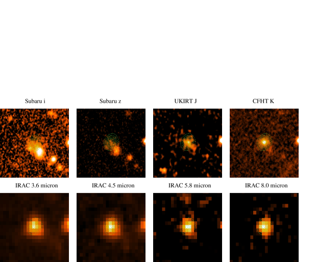
Figure 1.— Images of object 28 taken from the COSMOS survey. From upper left to lower right panels we show the images from Subaru $i^{+}$, Subaru $z^{+}$, UKIRT J, CFHT K and the four channels of Spitzer/IRAC. The size of the image is 5$\farcs$5 $\times$ 5$\farcs$5. We overlap the radio contours (green lines) at 1.4 GHz from VLA COSMOS data on the frames to show the position of the radio source.

During the visual check of the individual counterparts, two main problems emerge in the COSMOS broadband catalog: i) the presence of nearby sources, within the 3″ radius used for the aperture photometry, contaminating the broad band measurements of the genuine emission from the radio-galaxies of our sample; ii) the counterparts to the i-band object does not always correspond to the same object over the various bands. Object 28 is a clear example of this situation (see Fig. 1): from the J band to 8$\mu$m the brightest source in the field is coincident with the radio source, while in the $i^{+}$ and $z^{+}$ bands this is out-shined by a nearby object, causing an erroneous identification in the COSMOS catalog across the various bands. Furthermore, the presence of this neighbor also causes a strong (and dominant short-ward of the J band) contamination to the genuine flux of the radio-galaxy. Other examples of contamination and mis-identification are reported in Fig.2.

In order to amend these problems, we first perform a new 3″ aperture photometry properly centered on the position of the radio source, to isolate the genuine emission of the counterparts. In case of contamination from nearby source(s), we subtract from the flux resulting from the photometry centered on the radio source the emission from the neighbor(s), limiting to the fraction that falls into the 3″ aperture. When we cannot separate a source from a close source or when the counterpart is not visible in a given band, we measure an 1-$\sigma$ upper limit to the flux.

At 24 $\mu$m, when the counterpart of a source is not seen at the radio position, we use the detection limit of MIPS catalogs as upper-limit to the source flux. However, when a nearby source contaminates the emission of our target, we prefer to measure the upper-limit directly on the image at the radio position. In addition, in the NUV/FUV band, if the source is not detected in GALEX we prefer not to include upper limits in our analysis, because its corresponding flux is substantially higher than those at larger wavelengths.

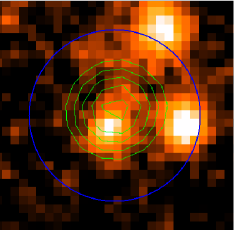
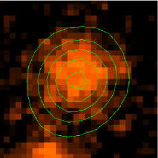
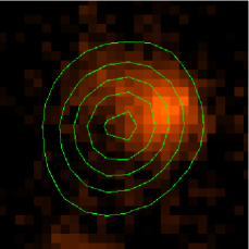
Figure 2.— Left panel: Subaru $i^{+}$ image of object 34 with superposed the radio contours (green) and the 3″ aperture centered on the radio source (blue). This is a case in which, in addition to the radio-galaxy, other objects lie inside the integration aperture of the target, contaminating the COSMOS catalog flux measurement. Middle and right panels: Subaru $z^{+}$ and CFHT $u^{*}$ images of object 5 with superposed the radio contours. This is a case of misidentification of a source with a neighbor included within the 1″ from the target) in different bands. The size of the images is 2″$\times$ 2″.

In some cases the GALEX photometry returns apparently incorrect results. In Fig. 3 we show as an example the HST and GALEX images of object 13; this source is labeled as detected by the COSMOS catalog in both the FUV and NUV GALEX bands, while clearly there is no emission above the background level. The opposite is seen in MIPS measurements, when clearly visible objects are missing from the catalog (see Fig. 4). In these cases, we do not consider the GALEX data, while for MIPS we provide a new estimate to the 24 $\mu$m flux.

We also find an apparent error in the reported UKIRT J-band photometric points. We obtain our own measurements on a sample of stars present in the COSMOS field (Wright et al., 2010) using the PSF-matched and PSF-original J-band images and we compare them to the magnitudes given by the catalog. This test reveals that the zero-point mag of the PSF-matched J-band images is higher than the corresponding value of the PSF-original J-band images, taking into account of the effect of the PSF convolution. This systematic difference of the zero-point magnitudes is $\Delta$J = 0.90$\pm$0.06, intriguingly similar to the offset between Vega and AB mag system for the UKIRT J-band (J_AB = J_Vega + 0.94 for UKIRT, Hewett et al. 2006). We obviate this problem by performing 3″-aperture photometry on the J-band counterparts on the UKIRT images smoothed with a Gaussian kernel to a 1.2-1.5″ FWHM to reproduce the effect of the PSF matching.

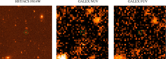
Figure 3.— From left to right: HST/ACS F814W, GALEX NUV and FUV bands images of object 13. The radio source (whose position is marked by the circles at the images center) does not apparently correspond to any UV emission, contrarily to the detection found in the catalog. The size of the images is 7$\farcs$5$\times$7$\farcs$5.

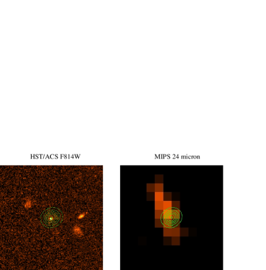
Figure 4.— Images of object 70 from ACS (left) and MIPS 24$\mu$m (right). This provides an example of a source clearly emitting at 24$\mu$m, but not present in the COSMOS Spitzer/MIPS catalog. The position of the radio source is represented by the green radio contours from VLA COSMOS. The size of the images is 28″$\times$28″.

Once we obtain the correct aperture photometry of the various multi-band counterparts of the radio galaxies, we apply the appropriate aperture corrections. While this is not needed for the Subaru, CFHT, and UKIRT, for GALEX data we apply an aperture correction by multiplying the total flux by a factor of 0.759 (Capak et al., 2007). Similarly, since we select from the IRAC catalog the 2$\farcs$9 aperture photometry (because it is closest to the 3″ aperture of the COSMOS broadband catalog among the different optional apertures), the IRAC aperture flux was converted to total source flux by using the aperture correction factors (from the IRAC manual) of 1.19, 1.27, 1.48, and 1.27 for the four channels. The MIPS data instead already include the aperture correction. Since the CFHT telescope is more sensitive and with higher resolution than the images from the NOAO telescopes, this usually results in far smaller errors for the K-band magnitudes. In such cases, we prefer to use only the CFHT K-band data. The results of the corrected 3″-aperture photometric measurements are tabulated in Tables 6 and 7.

5. SED fitting

The SEDs are derived by collecting multiband data from the FUV to the MIR. Since not all of the objects are detected in the entire set of available bands, the number of detections used to constrain the SED fitting ranges from 15 to 19.

The synthetic stellar templates used to model the observed SEDs are the Bruzual & Charlot (2009) (priv. comm.) and Maraston (2005) templates. These templates are defined with different Initial Mass Function (IMF) (Salpeter, 1955; Kroupa, 2001; Chabrier, 2003) with solar metallicity (Z_⊙ = 0.02). These libraries contain composite stellar population (CSP) computed with different star formation histories: a constant star-forming system (with constant star formation rate of 1 M_⊙/yr); a single burst of star formation; and ten $\mu$-models with time-decays of 0.1, 0.2, 0.3, 0.6, 1.0, 2.0, 3.0, 5.0, 10.0, and 15.0 Gyr. These templates include 221 tracks of ages from 0.1 Myr to 20 Gyr and cover the wavelength range from 91 Å  to 160 $\mu$m. Fig. 5 shows the stellar templates used for SED modeling.

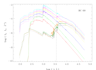
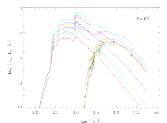
Figure 5.— Examples of SED templates from BC09 (Bruzual & Charlot, 2009) (left panel) and MA05 (Maraston, 2005) (right panel) in units of L_☉ $\AA^{-1}$. The templates correspond to different ages and different star formation histories. Arranging the BC09 and MA05 templates with increasing luminosity at 3550 Å  (following the dashed line), the different plotted models correspond to $\mu$=15 Gyr decaying CSP of 1.1 Myr (red line); single stellar population of 20 Gyr (gray line); $\mu$=0.1 Gyr decaying CSP of 10 Gyr (dark green line); $\mu$=10 Gyr decaying CSP of 2.8 Myr (light green line); $\mu$=0.3 Gyr decaying CSP 5.25 Gyr (orange line); $\mu$=5 Gyr decaying CSP of 6.9 Myr (blue line); $\mu$=3 Gyr decaying CSP of 17 Myr (yellow line); $\mu$=0.6 Gyr decaying CSP of 1.7 Gyr (pink line); $\mu$=2 Gyr decaying CSP of 38 Myr (fuchsia line); and $\mu$=1 Gyr decaying CSP of 0.2 Gyr (light blue line). We invite the reader to download the color version of the plot to distinguish the different lines.

The Bruzual & Charlot (2009) models differs from those of Maraston (2005) mainly because of a different recipe for the inclusion of thermally pulsing asymptotic giant branch (TP-AGB) phase. These stars significantly contribute to the IR emission for ages higher than $\sim$1 Gyr. The resulting effect is that the Bruzual & Charlot templates are bluer and give slightly older ages than Maraston (2005) models.

5.1. SED fitting method: Hyperz

We firstly estimate the photometric redshift for our sample by using the template fitting technique, Hyperz (Version 1.3 , obtained from M. Bolzonella in priv. comm.), described in detail by Bolzonella et al. (2000). This SED fitting procedure is based on reproducing the overall shape of the SEDs and recognizing strong spectral properties, such as the 4000 Å  Ca break or Lyman break at 912 Å. This code consists of a convolution of templates, which represent the rest-frame SEDs for galaxies with different star formation histories, with the filter response functions given by the COSMOS survey.

The basic assumption of this SED modeling is that the host galaxies of the radio sources in our sample are dominated by stellar emission. Thus the MIPS 24 $\mu$m photometric point is excluded because this emission is obviously not of stellar origin. Furthermore, object 236, a spectroscopically-confirmed QSO (see Sect. 5.3), is excluded from this analysis. The code also takes into account extinction (by using the reddening law from Calzetti et al. 2000) which is applied to the templates. The reddened templates are then shifted in wavelength searching for the correct redshift. The best fit is obtained through $\chi^{2}$ minimization. The grid spacings in redshift and in $A_{V}$ are 0.01 and 0.1, respectively. The Hyperz code gives the probability P($\chi_{rid}^{2}$) associated with $\chi_{rid}^{2}$ (i.e., the reduced $\chi^{2}$, which is defined as $\chi^{2}_{min}$/$\nu$, where $\nu$ is the number of degrees of freedom). Because we are essentially interested in the redshift (the other parameters are affected by the degeneracy), the degrees of freedom are N_filters - 1.

Similarly to Ilbert et al. (2009), we increase the flux errors by 10% when the probability associated with the $\chi_{rid}^{2}$ is less than 0.01. This factor does not shift the best-fit photo-z value but broadens the $\chi^{2}$ peak and derived redshift uncertainty. The program provides the redshift of the object measured at the different confidence intervals defined by the values of $\chi_{rid}^{2}$. We conservatively choose the solution at a 99% confidence level. Bolzonella et al. (2000) discussed the effects of degeneracy in the parameter space defined by star formation history, age, and reddening. However, they show that this does not strongly affect the value of the photometric redshift. Hyperzmass, a code which works in a similar way to Hyperz, returns the mass of the stellar population corresponding to the best fit and we adopt again the 99%-confidence level to quote the errors on the mass.

Fig. 15 (left panels) shows the SED fit obtained with Hyperz. The resulting properties from the modeling are listed in Table 3. Inspection of this figure indicates that Hyperz does not always return satisfactory results; indeed, in several cases, it cannot reproduce the bluest part of the spectrum (possibly due to a young stellar component) or the substantial SED “bump” at long wavelengths, clearly suggestive of dust emission and often extending even to the IRAC 3.6 $\mu$m measurements.

5.2. ‘2SPD’ fitting technique

In order to improve the quality of the SED fitting we developed a code that includes 2 Stellar Populations and Dust component (2SPD). More precisely, we take into account two different stellar populations, typically, one younger and one older (YSP and OSP, respectively). We model the dust component with a single (or, in a few cases, two) temperature black-body emission. Thus, at this stage, we can include the 24 $\mu$m MIPS flux in the fitting process.

The synthetic models used are the same as described in the previous section, but limiting to those with single stellar population with ages ranging from 1 Myr to 12.5 Gyr. We adopt a dust-screen model for the extinction normalized with the free parameter $A_{V}$, and the Calzetti et al. (2000) law.

The code searches for the best match between the sum of the different components (young and old stellar templates and dust emission) and the photometric points minimizing the appropriate $\chi^{2}$ function. 2SPD returns the following free parameters: $z$, $A_{V}$, the age of the two stellar populations, the temperature of the dust component(s), and the various normalization factors. From these quantities we measure the stellar mass content of the two stellar populations at 4800 Å rest frame. Similarly to the case of Hyperz, caution should be exerted before associating these values to physical quantities because of degeneracy in the parameter space, apart from the photometric redshifts.

To estimate the errors on the photo-z and mass derivations, we measure the 99%- confident solutions for these quantities. This is computed by varying the value the parameter of interest until the $\chi^{2}$ value increases by $\Delta\chi^{2}$ = 6.63, corresponding to a confidence level of 99% for that parameter.

Fig. 15 (righ panels) shows the outputs of 2SPD code, while Table 4 presents the resulting parameters of the fit.

The dust emission is usually poorly constrained. In many cases no excess above the stellar component is required at $\lambda<24\mu$m. In this case dust is needed only to account for the 24 $\mu$m data-point and often this measurement is an upper limit. The values reported in Table 4 correspond to the best fitting model for each galaxy and must be interpreted as approximate rather than real measurements of the dust emission properties. We will return to the dust properties in more detail in Sect. 6.4.

5.3. COSMOS photometric redshifts

As a comparison with our results we also collect the photometric redshifts from the COSMOS redshift catalog. Mobasher et al. (2007) provide photometric redshifts for 860,000 galaxies in the COSMOS field with $i^{+}$ $<$ 25. Their technique is based on a $\chi^{2}$ template-fitting procedure applied to the SEDs derived with up to 16 photometric points from the $u$ to the K band. To evaluate the reliability of the derived photometric redshifts, they compare them with spectroscopic redshifts from a sample of 868 galaxies in zCOSMOS with z $<$ 1.2. The rms scatter between photometric and spectroscopic redshifts is $\sigma_{(zphot-zspec)/(1+zspec)}$ = 0.031 with a small fraction of outliers (2.5%).

Ilbert et al. (2009) substantially improve this analysis by including data from 30 broad, intermediate, and narrow bands covering the wavelength range from UV to MIR. Redshifts are computed for 607,617 sources (with $i^{+}<$ 26). The method used by these authors accounts for the contribution of emission lines to the SEDs. Comparison with 4,148 zCOSMOS spectroscopic redshifts indicates a dispersion of $\sigma_{(zphot-zspec)/(1+zspec)}$ = 0.007 at $i^{+}_{AB}<$ 22.5. Nevertheless, the accuracy is strongly degraded at $i^{+}>$ 25.5. Table 1 shows the photometric redshifts measured by Ilbert et al. (2009).

Most of the radio galaxies of our sample are included in the COSMOS Photometric Redshift Catalog Fall 2008, which provides the photometric redshifts measured by Ilbert et al. (2009). We adopt again a 0$\farcs$3 search radius and find 29 objects. We report the results in Table 3. One of these objects (236) turns out to be a spectroscopically-confirmed QSO at z = 2.132 (Prescott et al., 2006). The attempt of Ilbert et al. (2009) to estimate its photometric redshift failed because the templates used by these authors were not suitable to fit its AGN-dominated SED. Similarly, Mobasher et al. (2007) provided for this object a tentative photometric redshift, which is z=1.23${}^{+0.03}_{-0.17}$, which is clearly inconsistent with the spectroscopic value.

6. RESUTS

The SED modeling process has been performed for all the objects (except for the spectroscopically-confirmed QSO, object 236), by using the two template-fitting techniques (Fig 15). As expected, 2SPD code has turned out to more reliably model the SEDs of our sources than Hyperz. This is crucial in UV band. In fact, when significant UV emission appears in the SED, such as, in objects 31, 258 and 285, Hyperz technique struggles to fit simultaneously such a UV component and the remaining part of SED, which is well represented by an OSP. In this case, the best fit result from Hyperz is obtained using an old composite stellar population. This is due to the fact that the $\chi^{2}$ is lower if only the the old component of the SED is fitted, rather than the UV data points which are less well represented. Conversely, as expected, 2SPD technique is more efficient to treat this case, since it just adds a small fraction of YSP to a dominant OSP to reproduce the UV emission, by departing from the concept of single star formation history.

Table 3Hyperz SED fitting

ID	redshift		CSP Template					Log M∗
	zphot,Hyperz	zphot,2SPD	type	SFH	Age	AV	$\chi_{rid}^{2}$	Log M⊙
1	0.85${}^{+0.05}_{-0.08}$	0.88${}^{+0.04}_{-0.05}$	BC	ssp	1.434	1.00	0.73	10.98${}^{+0.07}_{-0.04}$
2	1.31${}^{+0.14}_{-0.07}$	1.33${}^{+0.10}_{-0.09}$	BC	$\tau$=0.3	0.5088	2.9	1.43	11.00${}^{+0.09}_{-0.12}$
3	2.33${}^{+0.18}_{-0.18}$	2.20${}^{+0.32}_{-0.44}$	Ma	$\tau$=0.3	1.0152	1.0	11.50	10.43${}^{+0.07}_{-0.02}$
4	1.44${}^{+0.14}_{-0.30}$	1.37${}^{+0.10}_{-0.06}$	BC	$\tau$=0.1	0.3602	2.4	0.30	11.10${}^{+0.16}_{-0.09}$
5	1.93${}^{+0.06}_{-0.11}$	2.01${}^{+0.22}_{-0.35}$	Ma	const	2.0	2.3	9.57	11.68${}^{+0.21}_{-0.15}$
11	1.55${}^{+0.28}_{-0.15}$	1.57${}^{+0.14}_{-0.09}$	Ma	$\tau$=1.0	1.0152	0.8	0.51	11.05${}^{+0.11}_{-0.06}$
13	1.12${}^{+0.02}_{-0.01}$	1.19${}^{+0.08}_{-0.11}$	BC	ssp	0.1805	2.4	12.60	10.91${}^{+0.03}_{-0.03}$
16	1.04${}^{+0.06}_{-0.15}$	0.97${}^{+0.12}_{-0.07}$	BC	ssp	0.1805	2.2	0.78	10.58${}^{+0.10}_{-0.05}$
18	0.92${}^{+0.02}_{-0.02}$	0.92${}^{+0.14}_{-0.11}$	BC	ssp	0.1805	2.1	6.63	10.48${}^{+0.03}_{-0.04}$
20	0.80${}^{+0.20}_{-0.05}$	0.88${}^{+0.02}_{-0.02}$	BC	$\tau$=0.3	1.7	1.4	0.76	10.85${}^{+0.15}_{-0.08}$
22	1.21${}^{+0.09}_{-0.05}$	1.30${}^{+0.05}_{-0.04}$	BC	ssp	0.5088	3.8	3.83	10.52${}^{+0.87}_{-0.08}$
25	1.37${}^{+0.09}_{-0.12}$	1.33${}^{+0.11}_{-0.13}$	BC	ssp	0.1805	2.2	2.21	11.08${}^{+0.04}_{-0.11}$
26	1.09${}^{+0.05}_{-0.10}$	1.09${}^{+0.12}_{-0.07}$	BC	$\tau$=0.1	0.7187	1.8	1.75	11.29${}^{+0.01}_{-0.05}$
28	2.61${}^{+0.37}_{-0.22}$	2.90${}^{+0.20}_{-0.26}$	Ma	ssp	1.0152	0.64	3.31	11.73${}^{+0.03}_{-0.04}$
29	1.58${}^{+0.37}_{-0.17}$	1.32${}^{+0.23}_{-0.24}$	Ma	$\tau$=0.3	0.7187	1.0	0.89	10.36${}^{+0.14}_{-0.04}$
30	0.99${}^{+0.37}_{-0.11}$	1.06${}^{+0.11}_{-0.07}$	BC	$\tau$=0.3	1.7	1.8	1.14	11.10${}^{+0.14}_{-0.18}$
31	0.81${}^{+0.21}_{-0.18}$	0.88${}^{+0.03}_{-0.05}$	BC	$\tau$=0.3	0.7187	2.0	1.40	10.66${}^{+0.09}_{-0.04}$
32	3.11${}^{+0.21}_{-0.14}$	2.71${}^{+0.38}_{-0.34}$	BC	ssp	0.01	3.0	2.98	10.83${}^{+0.03}_{-0.08}$
34	1.50${}^{+0.56}_{-0.29}$	1.55${}^{+0.41}_{-0.19}$	Ma	$\tau$=15	2.0	2.0	0.60	10.85${}^{+0.64}_{-0.37}$
36	0.91${}^{+0.13}_{-0.08}$	1.07${}^{+0.10}_{-0.04}$	BC	$\tau$=0.6	0.0151	4.6	1.82	10.05${}^{+0.11}_{-0.21}$
37	2.04${}^{+0.15}_{-0.24}$	1.38${}^{+0.43}_{-0.42}$	Ma	ssp	0.0132	1.6	11.73	11.86${}^{+0.13}_{-0.03}$
38	1.34${}^{+0.14}_{-0.42}$	1.30${}^{+0.17}_{-0.28}$	Ma	ssp	0.01995	2.8	1.23	10.82${}^{+0.13}_{-0.17}$
39	0.80${}^{+0.23}_{-0.05}$	1.10${}^{+0.05}_{-0.05}$	BC	const	1.7	3.7	8.72	10.80${}^{+0.15}_{-0.12}$
52	0.75${}^{+0.12}_{-0.11}$	0.74${}^{+0.18}_{-0.19}$	BC	$\tau$=0.3	0.5088	2.0	1.60	10.54${}^{+0.19}_{-0.09}$
70	2.39${}^{+0.52}_{-0.14}$	2.32${}^{+0.53}_{-0.20}$	Ma	$\tau$=15.0	1.434	1.4	1.16	11.17${}^{+0.19}_{-0.12}$
202	0.95${}^{+0.44}_{-0.24}$	1.31${}^{+0.09}_{-0.12}$	BC	$\tau$=0.3	1.0152	2.6	0.83	10.60${}^{+0.28}_{-0.14}$
219	1.04${}^{+0.07}_{-0.15}$	1.03${}^{+0.02}_{-0.04}$	BC	ssp	0.1278	2.6	1.98	10.96${}^{+0.12}_{-0.01}$
224	1.07${}^{+0.11}_{-0.14}$	1.10${}^{+0.10}_{-0.04}$	BC	$\tau$=0.3	1.0152	2.0	0.85	10.92${}^{+0.12}_{-0.21}$
226	1.98${}^{+0.16}_{-0.27}$	2.35${}^{+0.63}_{-0.31}$	Ma	ssp	0.01	2.0	9.57	10.08${}^{+0.02}_{-0.05}$
228	1.30${}^{+0.09}_{-0.06}$	1.31${}^{+0.05}_{-0.07}$	BC	$\tau$=0.1	0.0263	4.2	1.25	10.35${}^{+0.20}_{-0.40}$
234	1.02${}^{+0.08}_{-0.04}$	1.10${}^{+0.14}_{-0.08}$	BC	ssp	0.1278	3.0	1.66	10.74${}^{+0.08}_{-0.01}$
258	0.83${}^{+0.11}_{-0.06}$	0.96${}^{+0.19}_{-0.13}$	BC	$\tau$=3.0	6.5	1.0	5.27	10.90${}^{+0.09}_{-0.07}$
285	1.22${}^{+0.13}_{-0.06}$	1.10${}^{+0.13}_{-0.08}$	BC	const	0.0151	2.8	4.56	10.03${}^{+0.18}_{-0.01}$

Table 42SPD SED fitting

ID	redshift	YSP				OSP		log M∗	Dust		IR excess		UV
	zphot	Age	AV	$f_{YSP}$	Log M∗	Age	AV		Tdust	Ldust	LIRexc.	$\alpha_{8-24}$	LUV
1	0.88${}^{+0.04}_{-0.05}$	0.02	0.80	1.5%	0.49%	4.0	0.15	10.08${}^{+0.04}_{-0.04}$	140	2.4	$<$43.31
2	1.33${}^{+0.10}_{-0.09}$	0.05	0.90	22.1%	1.3%	2.0	0.98	11.00${}^{+0.04}_{-0.04}$	156	7.4	$<$43.65		42.53
3	2.20${}^{+0.32}_{-0.44}$	0.03	0.12	6.5%	0.69%	1.0	0.00	10.59${}^{+0.08}_{-0.10}$	201-347	250-59	45.27	-0.01	43.21
4	1.37${}^{+0.10}_{-0.06}$	0.009	1.00	6.9%	0.24%	3.0	0.57	11.16${}^{+0.04}_{-0.03}$	100	5.2	$<$43.55		42.71
5	2.01${}^{+0.22}_{-0.35}$	0.02	1.80	53.1%	5.9%	3.0	0.93	11.49${}^{+0.04}_{-0.03}$	121	144.0	44.76	$>$0.49
11	1.57${}^{+0.14}_{-0.09}$	0.007	1.87	17.2%	0.62%	3.0	0.30	10.98${}^{+0.10}_{-0.05}$	98	15.4	$<$43.80
13	1.19${}^{+0.08}_{-0.11}$	0.03	1.17	16.2%	3.2%	1.0	0.58	10.72${}^{+0.04}_{-0.03}$	155-406	7.0-6.2	44.23	-0.41	42.65m
16	0.97${}^{+0.12}_{-0.07}$	0.006	1.16	14.8%	0.23%	2.0	0.52	10.74${}^{+0.06}_{-0.06}$	158	4.8	43.60	$>$-0.12	42.42m
18	0.92${}^{+0.14}_{-0.11}$	0.004	2.55	50.3%	13.5%	0.2	1.35	10.02${}^{+0.08}_{-0.08}$	116	13.9	$<$43.96
20	0.88${}^{+0.02}_{-0.02}$	0.002	1.26	3.7%	0.07%	3.0	0.42	11.03${}^{+0.02}_{-0.03}$	173	1.4	$<$43.02		42.25m
22	1.30${}^{+0.05}_{-0.04}$	0.04	1.18	10.1%	0.35%	2.0	1.50	11.16${}^{+0.02}_{-0.03}$	150	11.8	43.87	$>$0.66
25	1.33${}^{+0.11}_{-0.13}$	0.002	1.17	4.1%	0.28%	0.4	1.05	10.75${}^{+0.04}_{-0.05}$	138	8.8	43.75	$>$0.26	42.87m
26	1.09${}^{+0.12}_{-0.07}$	0.006	1.36	7.4%	0.17%	1.0	0.98	11.12${}^{+0.04}_{-0.04}$	128	3.9	$<$43.45		42.50m
28	2.90${}^{+0.20}_{-0.26}$	0.001	1.97	24.7%	3.9%	0.9	0.00	11.38${}^{+0.04}_{-0.04}$	146	47.4	44.28	$>$0.22
29	1.32${}^{+0.23}_{-0.24}$	0.004	0.38	11.9%	0.18%	0.4	0.94	10.03${}^{+0.05}_{-0.05}$	83	16.4	$<$43.68		42.83
30	1.06${}^{+0.11}_{-0.07}$	0.001	1.77	3.0%	0.13%	2.0	0.73	11.03${}^{+0.05}_{-0.05}$	130	3.5	$<$43.47
31	0.88${}^{+0.03}_{-0.05}$	0.007	0.23	7.5%	0.06%	2.0	0.23	10.75${}^{+0.03}_{-0.03}$	164	2.6	$<$43.35		42.86
32	2.71${}^{+0.38}_{-0.34}$	0.002	0.98	10.6%	0.26%	2.0	0.39	10.98${}^{+0.04}_{-0.04}$	205-452	51-58	44.96	-0.98	43.05
34	1.55${}^{+0.41}_{-0.19}$	0.005	0.55	11.0%	0.05%	3.0	0.51	10.99${}^{+0.07}_{-0.07}$	140	19.7	$<$44.04		42.82
36	1.07${}^{+0.10}_{-0.04}$	0.008	2.30	42.4%	2.0%	3.0	1.07	10.83${}^{+0.02}_{-0.03}$	186	4.4	43.46	$>$0.20
37	1.38${}^{+0.43}_{-0.42}$	0.001	0.00	1.0%	0.09%	0.3	0.09	10.61${}^{+0.11}_{-0.11}$	213-614	84-22	45.03	-0.25	44.10
38	1.30${}^{+0.17}_{-0.28}$	0.005	0.95	27.0%	0.58%	0.9	0.86	10.65${}^{+0.07}_{-0.07}$	260	6.2	43.77	0.45	43.03
39	1.10${}^{+0.05}_{-0.05}$	0.007	1.86	15.0%	0.83%	1.0	0.97	10.88${}^{+0.03}_{-0.03}$	80	5.3	$<$43.20
52	0.74${}^{+0.18}_{-0.19}$	0.004	0.66	13.6%	0.11%	2.0	0.34	10.78${}^{+0.10}_{-0.10}$	189	2.6	43.33	0.61	42.96
70	2.32${}^{+0.53}_{-0.20}$	0.009	0.48	12.8%	0.87%	0.4	0.74	10.65${}^{+0.07}_{-0.03}$	180	27.5	44.07	$>$-0.50	43.54
202	1.31${}^{+0.09}_{-0.12}$	0.005	0.14	1.2%	0.004%	3.0	0.14	10.86${}^{+0.03}_{-0.06}$	124	7.4	$<$43.66		42.21
219	1.03${}^{+0.02}_{-0.04}$	0.02	0.83	6.2%	0.69%	0.3	1.47	10.67${}^{+0.03}_{-0.03}$	112	2.8	$<$43.32		42.69m
224	1.10${}^{+0.10}_{-0.04}$	0.004	0.63	3.8%	0.04%	1.0	0.76	10.71${}^{+0.03}_{-0.04}$	155	4.5	$<$43.53		42.53m
226	2.35${}^{+0.63}_{-0.31}$	0.001	0.23	2.8%	0.12%	0.9	0.00	10.59${}^{+0.07}_{-0.09}$	212-467	88-36	45.01	-0.46	43.34
228	1.31${}^{+0.05}_{-0.07}$	0.002	2.29	37.1%	0.72%	2.0	2.21	11.06${}^{+0.03}_{-0.03}$	133	6.9	$<$43.64
234	1.10${}^{+0.14}_{-0.08}$	0.006	2.30	46.3%	2.2%	2.0	1.05	10.83${}^{+0.04}_{-0.04}$	104	5.8	$<$43.52
258	0.96${}^{+0.19}_{-0.13}$	0.001	0.08	1.6%	0.05%	0.08	1.72	10.64${}^{+0.08}_{-0.09}$	134	3.0	$<$43.41		43.27
285	1.10${}^{+0.13}_{-0.08}$	0.001	0.13	2.1%	0.05%	0.04	1.56	10.43${}^{+0.04}_{-0.04}$	135-448	1.9-1.8	43.73	-0.22	43.08

Table 5’Final’ redshifts and radio properties of the sample

ID	z	LNVSS	LFIRST	class
1	0.88s	$<$31.78	31.93	LP
2	1.33	32.02	32.4	LP
3	2.20	33.1	33.19	HP
4	1.37	32.77	32.86	HP
5	2.01	32.47	32.89	HP
11	1.57	$<$32.18	32.52	LP
13	1.19	32.02	32.22	LP
16	0.97s	32.38	32.27	LP
18	0.92	32.22	32.28	LP
20	0.88	$<$31.66	31.93	LP
22	1.30	$<$32.38	32.34	LP
25	1.33	32.29	32.39	LP
26	1.09	32.02	32.25	LP
28	2.90	32.99	33.13	HP
29	1.32	32.28	32.31	LP
30	1.06	31.83	32.11	LP
31	0.91s	32.14	32.18	LP
32	2.71	32.8	33.17	HP
34	1.55	32.84	32.77	HP
36	1.07	32.23	32.25	LP
37	1.38	32.26	32.33	LP
38	1.30	32.94	33.00	HP
39	1.10	$<$31.90	32.16	LP
52	0.74s	$<$31.54	31.73	LP
70	2.32	33.12	33.18	HP
202	1.31	31.98	32.46	LP
219	1.03	$<$31.96	32.09	LP
224	1.10	32.28	32.27	LP
226	2.35	$<$32.61	32.94	HP
228	1.31	32.25	32.51	LP
234	1.10	32.41	32.48	LP
236	2.13	33.29	33.29	HP
258	0.90s	31.90	32.12	LP
285	1.10	32.23	32.31	LP

6.1. Photometric redshifts

The first test on the accuracy of our photo-z derivation is a comparison with the spectroscopic redshifts, available for 6 objects (namely 1, 16, 25, 31, 52, and 258). They are all compatible with each other within the errors with the only exception of object 25. For this object the photometric redshifts measured with Hyperz and 2SPD (z = 1.37${}^{+0.09}_{-0.12}$ and z = 1.33${}^{+0.11}_{-0.13}$, respectively) are significantly different from the redshift inferred from its Magellan spectrum (z = 0.7917). However, the Magellan spectrum does not match with the COSMOS measurements, showing a large offset, of $\sim$0.8 dex. Apparently, the object observed by Magellan is not the radio galaxy 25 and we do not consider its spectroscopic-z as reliable. Reassuringly, we checked that the spectra and photometric data-points agree for the other 5 objects with available spectra.

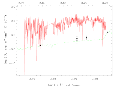
Figure 6.— Spectrum of object 25 (red solid line) from the Magellan survey (Trump et al., 2007) which provides a spectroscopic redshift of 0.7917. We overlap the synthetic SED (green dashed line) derived from Hyperz at redshift z = 1.37, fitting the photometric points. The wavelengths on the top corresponds to the observed wavelengths, and at the bottom to rest frame.

We then compare the photometric redshifts derived with the two SED fitting techniques. The overall range of $z$ is in both cases from $\sim$0.7 to $\sim$ 3. The median photo-z are 1.21 and 1.30 for Hyperz and 2SPD respectively. Generally, the photometric redshifts derived with the two methods are consistent with each other within the errors (Fig. 7, left panel). The normalized redshift differences ($\Delta z/(1+z)$) are smaller than 0.08 for all but 5 objects that reach $\Delta z/z\sim 0.12-0.15.$, and a single strong outlier (object 37, $\Delta z/z\sim 0.28$). For this galaxy, the Hyperz fit to the SED is particularly weak as it is not able to fit its photometric points at both FUV and MIR wavelengths.

Figure 7.— Comparison of the photometric-z measured with 2SPD with those obtained with Hyperz (left) and by Ilbert et al. (2009) (right).

Furthermore, we compare the photometric redshifts measured with our method and with the template-fitting technique of Ilbert et al. (2009). Objects 2, 22, 28, 32, and 36 are not involved in this comparison since they are not included in the Ilbert et al. (2009) sample. Fig. 7 (right panel) shows the comparison between the photo-z resulting from 2SPD and from Ilbert et al. (2009). Again, the two methods yield similar photometric redshifts with $\Delta z/(1+z)\lesssim 0.11$ for all but 2 objects, namely 226 and 228 for which we obtain $\Delta z/(1+z)=0.18$ and 0.25 respectively. In the case of object 226, similarly to the object 37 discussed above, the SED obtained with 2SPD reveals a strong excess at both UV and MIR wavelengths. Object 228 is instead a case of misidentification in the COSMOS multiband catalog. This result stresses the importance of our detailed work of identification to infer the genuine properties of the galaxies.

Therefore, unless a spectroscopic redshift is available, we generally prefer to use the photometric redshift obtained with 2SPD because our code also includes the dust component which turns out to be important in the SED modeling. Table 5 shows the redshifts used throughout all the paper.

6.2. Radio power distribution

Chiaberge et al. (2009) selected the sample in the COSMOS field looking for radio sources with radio luminosities below the FR I/FR II break. Since we now have improved estimates of the photometric redshifts of the objects, we can derive a more accurate value for their radio power. We show in Fig. 8 the histograms of K-corrected (using a radio spectral index $\alpha$ = 0.8) radio powers at 1.4 GHz measured with NVSS and FIRST. The resulting 1.4 GHz luminosities are in the range 10${}^{31.5}-10^{33.3}$ erg s^-1 Hz^-1. The local FR I/FR II break luminosity (Fanaroff & Riley, 1974), converted from 178 MHz to 1.4 GHz adopting $\alpha$ = 0.8, is L${}_{1.4\,\rm GHz}\sim 10^{32.6}$ erg s^-1 Hz^-1. Therefore, the radio distribution of our sample actually straddles the FR I/FR II break. Nonetheless we remind the reader that radio sources with a clear FR II morphologies were previously excluded by Chiaberge et al. (2009).

Figure 8.— Distribution of the K-corrected total radio luminosity (in erg s^-1 Hz^-1) at 1.4 GHz from the FIRST data (upper panel) and NVSS data (lower panel). The dashed lines corresponds to the local FR I/FR II break used to separate the sample in high power (HP, shaded histograms) and low power (LP) sources.

As already discussed by Chiaberge et al. (2009), the high-frequency radio observations available for this sample (their rest frame frequency are in the $\sim$ 3 - 5 GHz range) are not ideal to observe and detect their total radio structures because they miss diffuse/steep-spectrum radio emission. Lower frequency radio observations are needed for a more accurate measurement of their intrinsic total radio power distribution.

Since the radio power distribution is rather broad (covering two orders of magnitudes), we separate the sample into two groups, including sources of high and low power (HP and LP, respectively) using the local FR I/FR II break as divide (see Table 5). This operative definition enables us to explore the role of radio power in defining the overall properties of these galaxies. Two third of the sample shows radio luminosities below the break. The LP and HP classes are, not surprisingly, roughly separated also in redshifts (Fig. 9), since our sample is limited in radio flux, and indeed the HP sources generally lie at z $\gtrsim$ 1.5.

Figure 9.— Redshifts versus the K-corrected FIRST radio luminosity at 1.4 GHz (in erg s^-1 Hz^-1). The empty points are the LPs and the full points are the HPs.

6.3. Host galaxy properties inferred from SED modeling

We now focus on the properties of the host galaxies inferred from SED modeling and in particular on their stellar populations.

Figure 10.— Left panel: distribution of stellar masses (in M_⊙) of our sample obtained with 2SPD (upper panel) and with Hyperz (lower panel). Right panel: comparison between the stellar masses (in M_⊙) inferred from SED modeling using Hyperz and 2SPD techniques. The black histogram (points) represents the HPs, while the empty one the LPs.

One of the key and more robust result is the measurement of the stellar content, M_∗. The inferred mass range is $\sim$10${}^{10}-10^{12}$ M_⊙. The masses measured with Hyperzmass and with 2SPD are compared in Fig. 10. The two techniques return generally consistent values of the stellar masses for most sources (the median values are in both cases $\sim$ 7 $\times$ 10¹⁰ M_⊙), but with a few evident outliers. The stellar masses derived from single- and two- stellar components are know to differ significantly (e.g. Papovich et al. 2006). Furthermore, the inclusion of dust components by 2SPD has two effects by changing i) the stellar mass since thermal emission largely contributes to observed infrared emission, and ii) the photometric redshift. The largest outlier is object 37 whose SED is poorly fitted by Hyperz with a very high mass 7.0 $\times$ 10¹¹ M_⊙, while a strong dust component and a mass 10 times lower are required by 2SPD. At the opposite end of the mass distribution, we find two objects (36 and 226) in which again 2SPD finds a strong dust component, but where the Hyperz is a factor 3 to 7 lower than that obtained with 2SPD. Apparently, the presence of dust components has a stronger impact on the stellar mass estimate than the inclusion of a young stellar population.

Considering the radio power of the sources (see Fig. 11, left panel), HPs show slightly larger stellar mass content than LPs. The median values (obtained from 2SPD code) for LPs is 5.8 $\times$ 10¹⁰ M_⊙, while for HPs is 8.7 $\times$ 10¹⁰ M_⊙. However, the two distributions are very broad and show an almost complete overlap. A very similar result is found looking for differences in mass between objects at different redshifts (see Fig. 11, right panel).

Figure 11.— Stellar masses (in M_⊙) measured with 2SPD in relation with the K-corrected FIRST radio powers (in erg s^-1 Hz^-1) (left panel) and redshifts (right panel) of the sample. Empty points are LPs, while filled points are HPs.

Due to the degeneration inherent to the modeling of SEDs the remaining results of the stellar populations are relatively unconstrained. Overall, if we concentrate in the whole sample, the SED fitting shows that the hosts are mainly dominated by a massive OSP with an age of $\sim$ 1$-$3 $\times$ 10⁹ years. Although less reliable, the YSPs required to fit the UV excesses show ages of $1-30$ Myr, with a contribution to the total mass of the galaxy of $\lesssim 1\%$ for most sources. The flux contribution at 4800 Å (rest frame) of the YSP is $<$30% for most of the objects.

6.4. Dust emission

As discussed in Section 5.2, the parameters related to the dust emission must be taken as approximate rather than a real measurements of the dust component. Nonetheless, it is still significant that dust emission is required to adequately model the SEDs of 15 objects due to the detection of emission at 24 $\mu$m. In addition significant excesses above the stellar emission are observed also at shorter infrared wavelengths in 8 of these galaxies. In order to explore the dust properties we estimated the residuals between the best fitting model including only the stellar component and the data-points, looking for an excess at long wavelengths due to dust. We then integrated the residuals to obtain the total dust luminosity in the range covered by the Spitzer data, i.e. $\sim$ 3 - 26 $\mu$m. The integration is performed by assuming that the spectrum is represented by a multiple step function (see Fig. 12).

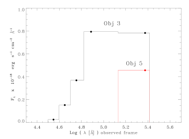
Figure 12.— Residuals obtained by subtracting the stellar component from the SED in the 5-bands Spitzer data which we ascribe to the dust emission. We show the results for object 3 (black) and 5 (red) as an example. The step function connecting the data-points is used to obtain the IR excess flux, i.e., the total dust flux.

The resulting dust luminosities (see Table 4), estimated as IR excess luminosities, are in the range $L_{\rm dust}\sim 10^{43.5}-10^{45.5}$ erg s^-1. A trend links radio and dust emission (see Fig. 13, left panel) with most (7/9) HP radio-sources showing a significant dust emission with luminosities larger than $L_{\rm dust}\sim 10^{44}$ erg s^-1. The LPs are instead (with only 2 exceptions) of lower L_dust and in many cases (16 galaxies) only upper limits can be derived.

We check the statistical significance of such a trend, by using a censored statistical analysis (ASURV, Lavalley et al. 1992) which takes into account of the presence of upper limits. Using the generalized Kendall’s $\tau$ test (Kendall, 1983), the probability that a fortuitous correlation appears is 0.0003. However, the common dependence of the two luminosities on redshift might play an important role. Therefore, we perform a partial correlation analysis (Akritas & Siebert, 1996) to examine the linear relation between the luminosities excluding the dependence on redshift. Operatively, we use the partial Kendall’s $\tau$ test, whose null hypothesis is the absence of the correlation excluding the redshift variable. The partial Kendall’s coefficient $\tau$ is 0.20 and the standard deviation is 0.081. The null hypothesis is then rejected at the level of 0.05.

We also measured the spectral index of the residuals between 8 $\mu$m and 24 $\mu$m, $\alpha_{(8-24)}$. Taking into account only significant excesses at 8 $\mu$m (residuals larger than 3 $\sigma$), this value can be estimated in 8 cases, with values spanning between $\alpha_{(8-24)}\sim$ 1 and -1. For the remaining objects with only a 24 $\mu$m detection, the limit to the 8 $\mu$m flux translates into a lower limit of $\alpha_{(8-24)}\gtrsim 1$. This parameter can be crudely related to the overall dust temperature. By assuming a single black-body dust component, the values of $\alpha_{(8-24)}$ translate into a temperature range of 500-850 K and 300-550 K for $\alpha_{(8-24)}=-1$ and $1$, respectively. The derived temperature depends on redshift, with the lower (upper) values of T being derived for $z=0.75$ ($z=2$).

Fig. 13 (middle panel) shows a broad relation between the IR spectral index and the IR excess luminosities. This would mean that the decrease of $\alpha_{(8-24)}$ is ascribable to the increase of the high-temperature dust component. Since a large radio power also implies a large dust luminosity, this may suggest a possible AGN nature of the dust heating source for the objects with largest IR excess.

Figure 13.— Infrared excess luminosity ($\>{\rm erg}\,{\rm s}^{-1}$) versus: (left panel) K-corrected FIRST radio luminosity ($\>{\rm erg}\,{\rm s}^{-1}$), and (right panel) spectral index from 8 to 24 $\mu$m estimated from the IR excess in the SED above the stellar emission. Empty points are the LPs and full points are the HPs.

6.5. UV excess

As noted in Sect. 5.1, the Hyperz code often does not reproduce satisfactorily the bluest part of the SED and we chose to model such part of spectrum with a young stellar population, included by our 2SPD. The inclusion of this component does not alter significantly the photometric redshift or the galaxies mass, but it is clearly of great importance to understand the nature of these radio galaxies. Nonetheless, inspection of the SEDs obtained with 2SPD indicates that the UV excesses (above the contribution of the old stellar component) are usually very poorly constrained. Furthermore, the very stellar origin is not granted and the UV excess might hide an AGN contribution.

It is necessary to introduce a model-independent criterion to assess which sources actually show an UV excess and to estimate its luminosity. We visually inspected all SEDs, searching for sources with a substantial flattening in the SED at short wavelengths or with a change of the slope between the OSP and the emission in the UV band. Fifteen sources show a clear UV excess (namely object 2, 3, 4, 29, 31, 32, 34, 37, 38, 52, 70, 202, 226, 258, and 285) and additional 7 objects show a marginal UV excess (namely object 13, 16, 20, 25, 26, 219, and 224). In the remaining galaxies the SEDs in UV bands drop sharply and are well reproduced by the emission from OSPs. In order to quantify the UV contribution, we measure the flux at 2000 Å in the rest frame, L_UV, from the best fitting model, for those objects showing the UV excess. The UV luminosities range is $10^{42}-10^{44}$ erg s^-1. HPs show larger UV luminosities than LPs by a factor 2.5, even though the strongest UV excess is seen in the LP radio galaxy 37. If we concentrate the sources which do not show an UV excess, the 2000 Å luminosity is $\lesssim 10^{43}$ erg s^-1 (mostly, $\sim 10^{42}$ erg s^-1).

In order to explore the nature of the UV emission, it is useful to compare the UV luminosity with the multiband properties obtained in the previous sections. No relations appear to link the UV excess to the redshift and the mass of the galaxy. Conversely, the UV luminosity appears to be linked to the radio power and IR excess luminosity (Fig. 14).

For the radio and UV luminosities the linear correlation coefficient is $r=0.404$ and the probability of the presence of a fortuitous relation is P= 0.062. The partial Kendall’s coefficient $\tau$ is 0.17 and the standard deviation is 0.15: the null hypothesis, i.e. the absence of the correlation, can not be rejected.

For the IR-UV relation, the generalized Kendall’s $\tau$ test returns a probability of no correlation of P= 0.0072. We obtain a partial Kendall’s coefficient $\tau$ = 0.41 and a standard deviation of 0.069: the null hypothesis, i.e. the absence of the correlation, is rejected at the level of 0.05.

Figure 14.— UV luminosity ($\>{\rm erg}\,{\rm s}^{-1}$) measured at 2000 Å  versus: (left panel) K-corrected FIRST radio luminosity ($\>{\rm erg}\,{\rm s}^{-1}$) , and (right panel) infrared excess luminosity ($\>{\rm erg}\,{\rm s}^{-1}$) . Empty points are the LPs and full points are the HPs.

7. Discussion and Conclusions

We used the multiwavelength data provided by the COSMOS survey to analyze the first sizeable sample of 34 low-power radio galaxies at high redshifts (z $\gtrsim$ 1), selected by Chiaberge et al. (2009). We performed a careful visual inspection of all their multiwavelength counterparts to identify their genuine emission and to infer their SEDs. Those would have been compromised in case of a blind use of the COSMOS catalog. Taking advantage of the FUV-MIR spectral coverage, we modeled their SEDs using two different template fitting techniques: i) the Hyperz code that uses a single stellar population and ii) our own code 2SPD that includes also dust component(s) and a young stellar population. We analyzed the properties of the SEDs of the sample. We here summarize the main results and briefly discuss them:

1. The photometric redshifts of these radio sources range from $\sim$0.7 to 3. The photo-z measured with the two techniques are generally consistent with each other, with those measured by Ilbert et al. (2009), and with the available spectroscopic redshifts. In addition, we measured the photometric redshifts for five objects which were not included in the Ilbert et al. (2009) sample.

2. The new and accurate measurements of the photometric redshifts enable us to infer the radio power distribution of these objects. The resulting K-corrected 1.4 GHz luminosities are in the range 10${}^{31.5}-10^{33.3}$ erg s^-1 Hz^-1, straddling the FR I/FR II break luminosity (L${}_{1.4\,\rm GHz}\sim 10^{32.6}$ erg s^-1 Hz^-1) as defined for low redshifts galaxies.

3. The resulting stellar masses are mostly confined in the range $\sim$10^10.5-11.5 M_⊙, with a median value of 7 $\times$ 10¹⁰ M_⊙.

4. The SED of most objects of the sample is consistent with the presence of a dominant contribution from an old stellar population with an age $\sim 1-3\times$ 10⁹ years. However, significant excesses are often observed at the shortest and/or longest wavelengths.

5. A dust component is needed to account for the 24 $\mu$m emission in 15 galaxies and significant excesses above the stellar emission are observed also at shorter infrared wavelengths in 8 of these galaxies. Estimates of the dust luminosity yield values in the range $L_{\rm dust}\sim 10^{43.5}-10^{45.5}$ erg s^-1. The overall dust temperature, estimated for the 8 radio-galaxies with a substantial dust excess at $\lambda\lesssim 8$$\mu$m, is in the range 300-850 K.

6. Inspection of the SED obtained with 2SPD indicates that the UV excesses (above the contribution of the old stellar component) are often present (significantly in 15 sources and marginally in 7 sources), but they are usually weakly constrained. The UV luminosities measured at 2000 Å (rest frame) is in the range $10^{42}-10^{44}$ erg s^-1.

7. Although the censored analysis does not provide significantly high statistical parameters, we can tentatively confirm the presence of positive links between the dust emission with both the radio and UV luminosities. For these relations, the possibility of a common luminosity dependence on distances is rejected at the level of 0.05.

The selection performed by Chiaberge et al. (2009) with the aim of searching for FR I candidates at z $\sim 1-2$ turned out to be successful. In fact, our work confirms i ) their location in the range of redshifts aimed with the selection process, although extending slightly below 1 and up to z $\sim$ 3 and ii) the low radio luminosity of the sample, generally consistent with those of the local FR I, although 1/3 of the sample exceeds the local FR I/FR II luminosity break. The extension of their radio power to larger luminosities does not necessarily imply a FR II nature for those sources. In fact the sources with a clear FR II morphology were excluded from the analysis. In addition, in the local Universe, the radio distribution of FR Is is broad and overlaps with the FR II distribution (Zirbel & Baum, 1995). Furthermore, this overlap increases at higher radio frequencies.

Overall, the hosts of these high-z low-luminosity radio-sources are similar to those of the local FR I which usually live in red massive early-type galaxies (e.g., Zirbel 1996; Best et al. 2005; Baldi & Capetti 2008; Smolčić 2009; Baldi & Capetti 2010).

However, the SED modeling reveals that additional components to the old stellar population have to be included to account for the emission at the SED extremes, i.e. in either the UV or in the MIR band, in most of the sources of the sample. This behavior is not seen in the low-z FR I that are generally faint in UV (both from the point of view of star formation and nuclear emission, Chiaberge et al. 2002; Baldi & Capetti 2008). Similarly, their MIR luminosities exceed by a very large factor (between 30 and 3000 for the MIR detected sources) the typical low-z FR I luminosities ($\sim 10^{42}\>{\rm erg}\,{\rm s}^{-1}$, Hardcastle et al. 2009). Conversely, the UV and MIR properties are somewhat similar to those of local FR IIs, which show bluer color (e.g., Baldi & Capetti 2008; Smolčić 2009) and large dust amount (e.g., de Koff et al. 2000; Dicken et al. 2010) than FR Is.

The origin of the MIR and UV emission can not be firmly established based on the available data. The estimate of the dust temperature (possible for only 8 objects) is in the range expected from dust heating from a quasar-like nucleus ($T\gtrsim 300$ K, e.g. Siebenmorgen et al. 2004; Ogle et al. 2006) and far larger than the dust associated with star formation (e.g., Hwang et al. 2010; Sreenilayam & Fich 2011; Boquien et al. 2011; Patel et al. 2011). The high end of the MIR luminosity reaches values similar to those found in high power radio-galaxies and QSOs. However, dust emission is seen only in less than half the sources of the sample.

Similarly, a UV component in excess to the old stellar population is firmly detected in the same number of sources (but there is not a one-to-one correspondence between UV and MIR emission). The observed UV luminosities are much larger that the faint non-thermal UV-nuclei seen in FR I and, instead, similar to those FR IIs (Chiaberge et al., 1999, 2002), dominated by the accretion disk emission.

Summing up, we find that the sources of the sample display a wide variety of properties, despite the relatively narrow range in radio luminosities. The 8 objects with the strongest MIR excess, and with high dust temperature indicative of a quasar-like nature, also show a significant UV excess. To this group we must obviously add the object 236, the spectroscopically confirmed QSO. We must note, however, that the SED of these 8 sources is much redder than that of object 236 and that their HST images do not provide any evidence for the presence of bright unresolved nuclei, as described by Chiaberge et al. (2009) based on visual inspection of the data.

At the opposite end of the radio luminosity distribution, there are 7 galaxies not showing any UV excess nor any 24 $\mu$m emission (and this number raises to 11 by including also the objects with only marginal UV excesses).

The remaining galaxies, amounting to about half of the sample, show an excess only in either the UV or MIR band. For those objects which do not show an UV excess or are not detected at 24 $\mu$m, the limits to the UV/MIR ratio are broadly consistent with the values obtained for the remaining galaxies of the sample. In particular we do not find objects with a high MIR luminosity without an UV excess that might be expected in the case of an obscured QSO. Unfortunately, with the available information we cannot distinguish between an origin related to star formation or to an active nucleus. In addition, relatively large amounts of dust, suggested by the dust luminosities, indicate that possible obscuration may prevent us from detecting UV emission.

A further detailed analysis of the nuclear properties is needed to understand which type of AGN are associated with these high-z radio galaxies. This will include their X-ray emission (Tundo et al., 2011) and the radio core flux, available from the COSMOS/VLA data, but which we defer to a future study. This might also provide new insights on the controversial FR I-QSO association (e.g., Falcke et al. 1995; Baum et al. 1995; Cao & Rawlings 2004; Blundell & Rawlings 2001, see also Blundell 2003 for review on this subject).

Summarizing, this work validates the first sizeable sample of low-luminosity radio galaxies at high redshifts, 0.7 $\lesssim$ z $\lesssim$ 3. This opens the possibility to perform a detailed comparison of the host and nuclear properties of these sources with those of i) the local low-luminosity radio-galaxies, ii) the powerful radio-galaxies in the same redshift range, and iii) the population of non active galaxies at $z\sim 1-3$. These issues will be addressed in a forthcoming paper.

$\begin{array}[]{ccc}\vspace{2em}\includegraphics[scale={0.33},angle={90}]{1cspnew.ps}&\includegraphics[scale={0.33},angle={90}]{sed1_2sp_dustnew.ps}\\ \vspace{1em}\includegraphics[scale={0.33},angle={90}]{2cspnew.ps}&\includegraphics[scale={0.33},angle={90}]{sed2_2sp_dustnew.ps}\\ \vspace{1em}\includegraphics[scale={0.33},angle={90}]{3cspnew.ps}&\includegraphics[scale={0.33},angle={90}]{sed3_2sp_2dustnew.ps}\\ \vspace{1em}\includegraphics[scale={0.33},angle={90}]{4cspnew.ps}&\includegraphics[scale={0.33},angle={90}]{sed4_2sp_dustnew.ps}\end{array}$

Figure 15.— Left panels: SEDs of the sample (green line) fitting the photometric points, as result of Hyperz. We plot the photometric point at 24 $\mu$m (Spitzer/MIPS), if available, but is not included in the modeling. Right panels: SEDs of the objects fitted with 2SPD. The total model is the green line, the YSP is the blue line, the OSP is the red line, and the dust component(s) is the light blue line. For both the panels, the wavelengths on top of the plots correspond to observed wavelengths, while those on bottom are at rest frame. For object 236 (QSO) we only show the photometric points.

$\begin{array}[]{ccc}\vspace{2em}\includegraphics[scale={0.33},angle={90}]{5cspnew.ps}&\includegraphics[scale={0.33},angle={90}]{sed5_2sp_dustnew.ps}\\ \vspace{1em}\includegraphics[scale={0.33},angle={90}]{11cspnew.ps}&\includegraphics[scale={0.33},angle={90}]{sed11_2sp_dustnew.ps}\\ \vspace{2em}\includegraphics[scale={0.33},angle={90}]{13cspnew.ps}&\includegraphics[scale={0.33},angle={90}]{sed13_2sp_2dustnew.ps}\\ \vspace{1em}\includegraphics[scale={0.33},angle={90}]{16cspnew.ps}&\includegraphics[scale={0.33},angle={90}]{sed16_2sp_dustnew.ps}\end{array}$

Figure 15.— Continued

$\begin{array}[]{ccc}\vspace{2em}\includegraphics[scale={0.33},angle={90}]{18cspnew.ps}&\includegraphics[scale={0.33},angle={90}]{sed18_2sp_dustnew.ps}\\ \vspace{1em}\includegraphics[scale={0.33},angle={90}]{20cspnew.ps}&\includegraphics[scale={0.33},angle={90}]{sed20_2sp_dustnew.ps}\\ \vspace{1em}\includegraphics[scale={0.33},angle={90}]{22cspnew.ps}&\includegraphics[scale={0.33},angle={90}]{sed22_2sp_dustnew.ps}\\ \vspace{1em}\includegraphics[scale={0.33},angle={90}]{25cspnew.ps}&\includegraphics[scale={0.33},angle={90}]{sed25_2sp_dustnew.ps}\end{array}$

Figure 15.— Continued

$\begin{array}[]{ccc}\vspace{2em}\includegraphics[scale={0.33},angle={90}]{26cspnew.ps}&\includegraphics[scale={0.33},angle={90}]{sed26_2sp_dustnew.ps}\\ \vspace{1em}\includegraphics[scale={0.33},angle={90}]{28cspnew.ps}&\includegraphics[scale={0.33},angle={90}]{sed28_2sp_dustnew.ps}\\ \vspace{1em}\includegraphics[scale={0.33},angle={90}]{29cspnew.ps}&\includegraphics[scale={0.33},angle={90}]{sed29_2sp_dustnew.ps}\\ \vspace{2em}\includegraphics[scale={0.33},angle={90}]{30cspnew.ps}&\includegraphics[scale={0.33},angle={90}]{sed30_2sp_dustnew.ps}\end{array}$

Figure 15.— Continued

$\begin{array}[]{ccc}\vspace{2em}\includegraphics[scale={0.33},angle={90}]{31cspnew.ps}&\includegraphics[scale={0.33},angle={90}]{sed31_2sp_dustnew.ps}\\ \vspace{1em}\includegraphics[scale={0.33},angle={90}]{32cspnew.ps}&\includegraphics[scale={0.33},angle={90}]{sed32_2sp_2dustnew.ps}\\ \vspace{2em}\includegraphics[scale={0.33},angle={90}]{34cspnew.ps}&\includegraphics[scale={0.33},angle={90}]{sed34_2sp_dustnew.ps}\\ \vspace{1em}\includegraphics[scale={0.33},angle={90}]{36cspnew.ps}&\includegraphics[scale={0.33},angle={90}]{sed36_2sp_dustnew.ps}\end{array}$

Figure 15.— Continued

$\begin{array}[]{ccc}\vspace{2em}\includegraphics[scale={0.33},angle={90}]{37cspnew.ps}&\includegraphics[scale={0.33},angle={90}]{sed37_2sp_2dustnew.ps}\\ \vspace{1em}\includegraphics[scale={0.33},angle={90}]{38cspnew.ps}&\includegraphics[scale={0.33},angle={90}]{sed38_2sp_dustnew.ps}\\ \vspace{1em}\includegraphics[scale={0.33},angle={90}]{39cspnew.ps}&\includegraphics[scale={0.33},angle={90}]{sed39_2sp_dustnew.ps}\\ \vspace{1em}\includegraphics[scale={0.33},angle={90}]{52cspnew.ps}&\includegraphics[scale={0.33},angle={90}]{sed52_2sp_dustnew.ps}\end{array}$

Figure 15.— Continued

$\begin{array}[]{ccc}\vspace{2em}\includegraphics[scale={0.33},angle={90}]{70cspnew.ps}&\includegraphics[scale={0.33},angle={90}]{sed70_2sp_dustnew.ps}\\ \vspace{1em}\includegraphics[scale={0.33},angle={90}]{202cspnew.ps}&\includegraphics[scale={0.33},angle={90}]{sed202_2sp_dustnew.ps}\\ \vspace{1em}\includegraphics[scale={0.33},angle={90}]{219cspnew.ps}&\includegraphics[scale={0.33},angle={90}]{sed219_2sp_dustnew.ps}\\ \vspace{2em}\includegraphics[scale={0.33},angle={90}]{224cspnew.ps}&\includegraphics[scale={0.33},angle={90}]{sed224_2sp_dustnew.ps}\end{array}$

Figure 15.— Continued

$\begin{array}[]{cccc}\vspace{2em}\includegraphics[scale={0.33},angle={90}]{226cspnew.ps}&\includegraphics[scale={0.33},angle={90}]{sed226_2sp_2dustnew.ps}\\ \vspace{1em}\includegraphics[scale={0.33},angle={90}]{228cspnew.ps}&\includegraphics[scale={0.33},angle={90}]{sed228_2sp_dustnew.ps}\\ \vspace{2em}\includegraphics[scale={0.33},angle={90}]{234cspnew.ps}&\includegraphics[scale={0.33},angle={90}]{sed234_2sp_dustnew.ps}\\ \vspace{1em}\includegraphics[scale={0.33},angle={90}]{236cspnew.ps}&\end{array}$

Figure 15.— Continued

$\begin{array}[]{cc}\vspace{2em}\includegraphics[scale={0.33},angle={90}]{258cspnew.ps}&\includegraphics[scale={0.33},angle={90}]{sed258_2sp_dustnew.ps}\\ \vspace{2em}\includegraphics[scale={0.33},angle={90}]{285cspnew.ps}&\includegraphics[scale={0.33},angle={90}]{sed285_2sp_2dustnew.ps}\end{array}$

Figure 15.— Left panels: SEDs of the sample (green line) fitting the photometric points, as result of Hyperz. We plot the photometric point at 24 $\mu$m (Spitzer/MIPS), if available, but is not included in the modeling. Right panels: SEDs of the objects fitted with 2SPD. The total model is the green line, the YSP is the blue line, the OSP is the red line, and the dust component(s) is the light blue line. For both the panels, the wavelengths on top of the plots correspond to observed wavelengths, while those on bottom are at rest frame. For object 236 (QSO) we only show the photometric points

Table 6COSMOS multiwavelength counterparts of the sample

ID	$u^{*}$	$B_{J}$	$g^{+}$	$V_{J}$	$r^{+}$	$i^{*}$	$i^{+}$	$F814W$	$z^{+}$	$J$	$K_{S}$	$K$
(1)	(2)	(3)	(4)	(5)	(6)	(7)	(8)	(9)	(10)	(11)	(12)	(13)
1	26.56$\pm$0.15	25.89$\pm$0.13	25.61$\pm$0.10	24.42$\pm$0.05	23.55$\pm$0.03	22.24$\pm$0.05	22.29$\pm$0.11∗	21.87$\pm$0.06	21.32$\pm$0.01	20.46$\pm$0.10∗	19.59$\pm$0.09∗	19.57$\pm$0.03
2	26.79$\pm$0.20∗	26.43$\pm$0.11∗	26.29$\pm$0.11∗	25.93$\pm$0.10∗	25.26$\pm$0.08∗	24.35$\pm$0.45∗	24.43$\pm$0.10∗	24.49$\pm$0.34∗	23.44$\pm$0.07∗	22.18$\pm$0.15∗	20.85$\pm$0.02	20.90$\pm$0.15
3	26.69$\pm$0.17	25.58$\pm$0.10	25.81$\pm$0.12	25.60$\pm$0.11	25.53$\pm$0.10	25.31$\pm$0.78	25.10$\pm$0.08	24.96$\pm$0.79	24.48$\pm$0.12	23.39$\pm$0.25∗	21.57$\pm$0.03	22.84$\pm$0.96
4	26.64$\pm$0.17	25.93$\pm$0.13	25.88$\pm$0.13	25.46$\pm$0.10	25.12$\pm$0.08	24.27$\pm$0.36	24.20$\pm$0.05	23.82$\pm$0.29	23.27$\pm$0.04	21.93$\pm$0.10∗	20.53$\pm$0.01	20.74$\pm$0.16
5	$<$25.77∗	$<$25.68∗	$<$25.53∗	$<$25.17∗	$<$25.23∗	24.12$\pm$0.27	24.59$\pm$0.41∗	23.98$\pm$0.33	23.41$\pm$0.25	22.24$\pm$0.13∗	20.65$\pm$0.12	20.82$\pm$0.15
11	$<$29.40∗	28.75$\pm$1.14	28.00$\pm$0.76	27.11$\pm$0.35	26.27$\pm$0.17	25.16$\pm$0.84	24.96$\pm$0.07	24.64$\pm$0.60	24.09$\pm$0.08	22.28$\pm$0.07∗	21.18$\pm$0.16	21.75$\pm$0.49
13	26.14$\pm$0.15∗	25.75$\pm$0.13∗	25.74$\pm$0.13	25.02$\pm$0.09∗	24.38$\pm$0.06∗	23.20$\pm$0.17	23.29$\pm$0.04∗	22.90$\pm$0.13	22.21$\pm$0.02	21.44$\pm$0.09∗	20.46$\pm$0.10	20.54$\pm$0.16
16	26.07$\pm$0.12	25.71$\pm$0.12	25.32$\pm$0.11	24.84$\pm$0.08	24.23$\pm$0.05	23.10$\pm$0.14	23.15$\pm$0.03	22.85$\pm$0.10	22.16$\pm$0.02	21.47$\pm$0.08∗	20.40$\pm$0.08	20.50$\pm$0.11
18	26.16$\pm$0.13∗	25.76$\pm$0.10∗	25.51$\pm$0.10	24.61$\pm$0.08∗	23.99$\pm$0.06∗	22.91$\pm$0.11∗	22.80$\pm$0.04∗	22.51$\pm$0.10∗	22.04$\pm$0.03∗	21.54$\pm$0.07∗	20.71$\pm$0.04	20.92$\pm$0.18
20	26.11$\pm$0.15	25.74$\pm$0.15	25.51$\pm$0.10	24.57$\pm$0.06	23.67$\pm$0.04	22.35$\pm$0.09	22.40$\pm$0.02	22.19$\pm$0.08	21.53$\pm$0.02	20.79$\pm$0.06∗	19.91$\pm$0.07	20.10$\pm$0.07
22	$<$27.38∗	$<$27.44∗	$<$26.97∗	$<$26.85∗	$<$26.00∗		$<$25.13∗		23.93$\pm$0.06	22.14$\pm$0.17∗	20.79$\pm$0.10	21.24$\pm$0.15
25	26.66$\pm$0.22	25.36$\pm$0.09	25.44$\pm$0.10	24.97$\pm$0.07	24.55$\pm$0.05	23.64$\pm$0.32	23.52$\pm$0.03	23.32$\pm$0.19	22.57$\pm$0.03	21.43$\pm$0.09∗	20.57$\pm$0.05	20.59$\pm$0.17
26	26.58$\pm$0.20	25.44$\pm$0.10	25.56$\pm$0.10	24.92$\pm$0.07	23.90$\pm$0.04	22.68$\pm$0.10	22.60$\pm$0.02	22.32$\pm$0.09	21.57$\pm$0.01	20.42$\pm$0.04∗	19.42$\pm$0.03	19.48$\pm$0.04
28	$<$27.39∗	$<$27.50∗	$<$27.20∗	$<$26.90∗	$<$26.80∗		25.55$\pm$0.30∗		24.27$\pm$0.20∗	22.48$\pm$0.20∗	20.99$\pm$0.08∗
29	25.81$\pm$0.12	25.51$\pm$0.10	25.49$\pm$0.09	25.31$\pm$0.09	25.18$\pm$0.08	25.00$\pm$0.87	24.78$\pm$0.07	24.92$\pm$0.74	24.30$\pm$0.11	22.86$\pm$0.27∗	22.19$\pm$0.10	22.89$\pm$0.80
30	27.85$\pm$0.63	26.77$\pm$0.22	26.82$\pm$0.23	25.90$\pm$0.13	24.69$\pm$0.06	23.41$\pm$0.19	23.41$\pm$0.03	23.01$\pm$0.15	22.32$\pm$0.02	21.25$\pm$0.08∗	20.02$\pm$0.04	20.19$\pm$0.09
31	24.75$\pm$0.08	24.50$\pm$0.06	24.51$\pm$0.05	23.94$\pm$0.04	23.42$\pm$0.03	22.33$\pm$0.08	22.33$\pm$0.02	22.07$\pm$0.07	21.61$\pm$0.02	20.97$\pm$0.08∗	20.12$\pm$0.05	20.32$\pm$0.09
32	$<$27.54∗	27.85$\pm$0.48∗	$<$27.19∗	$<$27.00∗	26.44$\pm$0.30∗		26.07$\pm$0.25∗		25.15$\pm$0.28∗	24.13$\pm$0.50∗	22.43$\pm$0.17∗	23.24$\pm$1.44
34	26.09$\pm$0.40∗	26.19$\pm$0.20∗	26.00$\pm$0.19∗	25.58$\pm$0.12∗	25.44$\pm$0.10∗	25.09$\pm$0.66∗	24.88$\pm$0.07∗	24.95$\pm$0.25∗	24.12$\pm$0.11∗	23.10$\pm$0.51∗	21.10$\pm$0.29∗	20.96$\pm$0.14
36	$<$27.8∗	$<$26.80∗	$<$26.40∗	26.18$\pm$0.45∗	25.50$\pm$0.31∗	24.31$\pm$0.33∗	24.15$\pm$0.15∗	24.00$\pm$0.25∗	23.20$\pm$0.24∗	22.04$\pm$0.15∗	20.62$\pm$0.07	20.44$\pm$0.10
37	22.70$\pm$0.02	22.35$\pm$0.02	22.63$\pm$0.02	22.38$\pm$0.02	22.18$\pm$0.02	21.93$\pm$0.05	21.93$\pm$0.01		21.17$\pm$0.01	20.31$\pm$0.05∗	20.14$\pm$0.11∗	20.06$\pm$0.08
38	25.50$\pm$0.10	25.00$\pm$0.08	24.96$\pm$0.07	24.66$\pm$0.06	24.20$\pm$0.04	23.58$\pm$0.32	23.49$\pm$0.03	23.47$\pm$0.22	22.69$\pm$0.03	22.08$\pm$0.16∗	20.89$\pm$0.05	21.34$\pm$0.22
39	$<$27.07∗	26.05$\pm$0.15∗	$<$26.00∗	25.28$\pm$0.09	24.42$\pm$0.05	23.13$\pm$0.18	23.13$\pm$0.03	22.86$\pm$0.15	22.18$\pm$0.02	21.06$\pm$0.08∗	19.99$\pm$0.04	20.27$\pm$0.09
52	24.24$\pm$0.04	23.64$\pm$0.04	23.76$\pm$0.04	23.13$\pm$0.03	22.62$\pm$0.02	21.62$\pm$0.05	21.67$\pm$0.01	21.52$\pm$0.05	21.18$\pm$0.01	20.58$\pm$0.05∗	19.79$\pm$0.04	19.78$\pm$0.06
70	26.16$\pm$0.14∗	25.14$\pm$0.09∗	25.27$\pm$0.14∗	24.79$\pm$0.08∗	24.51$\pm$0.06	24.34$\pm$0.58	24.35$\pm$0.06	24.13$\pm$0.43	24.01$\pm$0.09	23.42$\pm$0.50∗	21.76$\pm$0.09	21.40$\pm$0.27
202	27.03$\pm$0.28	27.11$\pm$0.29	27.40$\pm$0.42	26.92$\pm$0.29	25.86$\pm$0.12	24.44$\pm$0.53	24.41$\pm$0.06	24.29$\pm$0.45	23.48$\pm$0.05	22.19$\pm$0.17∗	21.07$\pm$0.05	21.62$\pm$0.30
219	25.68$\pm$0.10	25.09$\pm$0.08	25.23$\pm$0.08	24.49$\pm$0.05	23.81$\pm$0.04	22.74$\pm$0.09	22.71$\pm$0.02	22.37$\pm$0.09	21.70$\pm$0.02	21.02$\pm$0.06∗	19.93$\pm$0.04	20.15$\pm$0.37
224	26.40$\pm$0.18	25.75$\pm$0.13	25.52$\pm$0.10	25.36$\pm$0.09	24.62$\pm$0.06	23.52$\pm$0.27	23.49$\pm$0.03		22.50$\pm$0.03	21.31$\pm$0.08∗	20.39$\pm$0.04	20.49$\pm$0.18
226	25.40$\pm$0.11	25.30$\pm$0.09	25.48$\pm$0.11	25.23$\pm$0.09	25.17$\pm$0.08	24.59$\pm$1.00	24.75$\pm$0.08	24.78$\pm$0.68	24.37$\pm$0.11	23.41$\pm$0.46∗	21.90$\pm$0.10	21.75$\pm$0.36
228	$<$28.50∗	$<$27.70∗	$<$27.70∗	$<$26.80∗	26.17$\pm$0.16		25.17$\pm$0.10	25.17$\pm$0.67	24.38$\pm$0.11	23.10$\pm$0.40∗	21.14$\pm$0.06	21.23$\pm$0.22
234	27.40$\pm$0.51∗	26.43$\pm$0.22∗	26.65$\pm$0.28∗	25.50$\pm$0.12∗	24.88$\pm$0.08∗	23.76$\pm$0.30	23.52$\pm$0.08∗		22.76$\pm$0.03	21.38$\pm$0.20∗	20.31$\pm$0.11∗	20.57$\pm$0.39
236	20.92$\pm$0.01	20.73$\pm$0.01	21.02$\pm$0.01	20.59$\pm$0.01	20.65$\pm$0.01	20.32$\pm$0.02		20.26$\pm$0.02	19.94$\pm$0.01	20.05$\pm$0.04∗	19.27$\pm$0.02	19.32$\pm$0.04
258	24.01$\pm$0.04	23.54$\pm$0.04	23.70$\pm$0.03	23.19$\pm$0.03	22.68$\pm$0.02	21.87$\pm$0.06	21.85$\pm$0.01	21.56$\pm$0.04	21.11$\pm$0.01	20.61$\pm$0.05∗	19.62$\pm$0.04	19.71$\pm$0.04
285	24.60$\pm$0.18∗	24.65$\pm$0.15∗	24.63$\pm$0.24∗	23.88$\pm$0.14∗	23.70$\pm$0.12∗	23.32$\pm$0.28	23.06$\pm$0.10∗		22.36$\pm$0.11∗	21.80$\pm$0.13∗	20.78$\pm$0.10∗	20.84$\pm$0.10

Note. — Column description: (1) ID number of the object; (2)-(3) right ascension and declination of radio source; (4) photometric redshifts found by Ilbert et al. (2009); (5) spectroscopic redshift: $a$ from zCOSMOS survey (Lilly et al., 2007), $b$ form Magellan survey (Trump et al., 2007), and $c$ from Prescott et al. (2006). The spectroscopic redshift of object 25 (marked with $*$) is considered incorrect (see Section 6.1); (6)-(7) flux at 1.4 GHz from NVSS (from http://www.cv.nrao.edu/nvss/NVSSlist.shtml) and FIRST (taken from Chiaberge et al. 2009) catalogs in mJy.

Note. — List of the filters used for our analysis, the associated telescopes, the effective wavelengths $\lambda_{eff}$, the PSF full-width half maximum (FWHM) of the images in each band, and their sensitivities at 5$\sigma$ (mag).

Note. — Results from the analysis of the SEDs of the sample with Hyperz. Column description: (1) ID number of the object; (2) photometric redshift as result of Hyperz; all errors are quoted at at 99% of confidence level; (3) photometric redshifts obtained with 2SPD; (4) source library of the best template which fits the observed SED: BC from Bruzual & Charlot (2009) and MA from Maraston (2005); (5) star formation history of the best template: $ssp$ corresponds to a single stellar population and $\tau$ = ’N’ corresponds to the $\mu$-models with exponentially decaying star formation rate with star formation timescale $\tau$ = N Gyr; (6) age of the best template in Gyr; (7) $A_{V}$ associated with the best template; (8) $\chi_{rid}^{2}$ of the best template; (9) stellar mass and its error of the galaxy in $Log\,M_{\odot}$ as result of Hyperzmass.

Note. — Results from the analysis of the SEDs with 2SPD. Column description: (1) ID number of the object; (2) photometric redshift measured with 2SPD; (3)-(4)-(5)-(6) age in Gyr, A_V, flux fraction and mass fraction of the young stellar population (YSP) at 4800 Årest frame; (7)-(8) age in Gyr and A_V of the old stellar population (OSP); (9) the total stellar mass of the galaxy in M_⊙; (10)-(11) the effective temperature (in K) of the one or two dust components and their luminosities, L_dust (in units of 10⁹ L_⊙); (12)-(13) the infrared excess luminosity (in erg s^-1) defined in the text (Section 6.4) and the spectral index measured on the infrared excess at 8 and 24$\mu$m; (14) UV luminosity at 2000 Å  in the rest frame in erg s^-1. The marginal UV excesses are marked with a ^m.

Note. — Column description: (1) ID number of the object; (2) redshift of the object used throughout the work, with the spectroscopic redshifts marked with a ^s; (3)-(4) K-corrected radio luminoisty at 1.4 GHz from NVSS (from http://www.cv.nrao.edu/nvss/NVSSlist.shtml) and FIRST (taken from Chiaberge et al. 2009) in erg s^-1 Hz^-1; (5) classification based on the radio power: low or high power (LP or HP) radio sources.

Note. — Column description: (1) ID number of the object; (2) CFHT $u^{*}$ magnitude with its error; (3)-(4)-(5)-(6) Subaru $B_{J}$, $g^{+}$, $V_{J}$, $r^{+}$ magnitudes with their errors; (7) CFHT $i^{*}$ magnitude with its error; (8) Subaru $i^{+}$ magnitude with its error; (9) HST/ACS $F814W$ magnitude with its error; (10) Subaru $z^{+}$ magnitude with its error; (11) UKIRT $J$ magnitude with its error; (12) CFHT $K$ magnitude with its error; (13) NOAO$K_{S}$ with its error. The values marked by $*$ are measured by our 3″-aperture photometry on the images.

Table 7COSMOS multiwavelength counterparts of the sample

ID	$FUV$	$NUV$	$IRAC1$	$IRAC2$	$IRAC3$	$IRAC4$	$MIPS$
1			54.89$\pm$0.23∗	36.50$\pm$0.29∗	23.87$\pm$0.97∗	14.73$\pm$2.07∗	$<$0.15
2			41.44$\pm$0.19	45.75$\pm$0.30	28.07$\pm$0.99	21.8$\pm$2.49	$<$0.15
3			13.65$\pm$0.15	23.62$\pm$0.25	55.88$\pm$0.94	166.89$\pm$1.98	1.47$\pm$0.02
4			42.97$\pm$0.19	48.78$\pm$0.29	37.71$\pm$1.04	29.34$\pm$2.19	$<$0.08
5			66.44$\pm$0.19	89.03$\pm$0.29	91.57$\pm$0.99	63.65$\pm$1.97	0.87$\pm$0.02
11			25.34$\pm$0.17	29.34$\pm$0.26	25.07$\pm$1.00	9.64$\pm$1.98	$<$0.15
13			49.51$\pm$0.18	51.39$\pm$0.26	53.24$\pm$0.98	75.84$\pm$2.04	0.32$\pm$0.03
16			44.29$\pm$0.18	32.54$\pm$0.28	26.19$\pm$0.94	18.39$\pm$2.26	0.22$\pm$0.02
18			31.03$\pm$0.17	24.94$\pm$0.28	18.13$\pm$0.99	14.03$\pm$2.15	$<$0.61∗
20			63.11$\pm$0.18	44.73$\pm$0.27	25.12$\pm$0.90	17.46$\pm$2.06	$<$0.08
22			57.27$\pm$ 0.17	64.90$\pm$0.29	41.55$\pm$0.89	32.84$\pm$2.16	0.25$\pm$0.03∗
25			49.17$\pm$0.19	55.52$\pm$0.28	38.82$\pm$0.99	25.08$\pm$2.19	0.18$\pm$0.05∗
26			126.74$\pm$0.25	108.17$\pm$0.29	59.54$\pm$0.98	44.75$\pm$1.92	$<$0.15
28			32.46$\pm$0.16	39.98$\pm$0.26	46.73$\pm$0.91	40.34$\pm$1.98	0.15$\pm$0.02
29			9.81$\pm$0.16	10.17$\pm$0.25	6.50$\pm$1.00∗	$<$7.38∗	$<$0.15
30			74.26$\pm$0.19	58.67$\pm$0.28	33.32$\pm$0.91	22.76$\pm$2.05	$<$0.15
31		25.15$\pm$0.24	47.86$\pm$0.16	34.60$\pm$0.25	24.98$\pm$0.81	19.36$\pm$1.78	$<$0.15
32			16.97$\pm$0.15	32.41$\pm$0.24	58.17$\pm$0.95	98.81$\pm$1.81	0.26$\pm$0.02
34			22.80$\pm$0.44∗	26.73$\pm$0.48∗	25.44$\pm$1.10∗	12.07$\pm$2.40∗	$<$0.26∗
36			49.50$\pm$0.16	43.80$\pm$0.27	30.24$\pm$0.87	21.89$\pm$1.97	0.15$\pm$0.04∗
37		23.55$\pm$0.15	88.32$\pm$0.22	123.39$\pm$0.32	158.41$\pm$1.10	249.52$\pm$2.18	1.58$\pm$0.39
38			30.47$\pm$0.17	28.00$\pm$0.28	29.99$\pm$0.95	24.94$\pm$2.35	0.13$\pm$0.06∗
39			74.19$\pm$0.21	66.35$\pm$0.32	34.74$\pm$0.96	25.29$\pm$2.40	$<$0.08
52		24.97$\pm$0.21	59.84$\pm$0.21	41.39$\pm$0.28	36.37$\pm$1.09	28.67$\pm$2.04	0.16$\pm$0.02
70			17.58$\pm$0.16	20.57$\pm$0.26	29.83$\pm$1.04	21.32$\pm$2.17	0.13$\pm$0.03∗
202			24.81$\pm$0.14	22.02$\pm$0.24	15.90$\pm$0.84	6.46$\pm$1.87	$<$0.15
219			98.71$\pm$0.23	86.12$\pm$0.32	48.50$\pm$1.02	38.60$\pm$2.26	0.12$\pm$0.01
224			48.09$\pm$0.17	41.65$\pm$0.26	25.56$\pm$0.88	18.53$\pm$2.07	$<$0.15
226			16.94$\pm$0.15	30.93$\pm$0.28	53.89$\pm$0.89	104.92$\pm$2.16	0.54$\pm$0.02
228			39.72$\pm$0.18	47.82$\pm$0.27	36.06$\pm$0.99	23.46$\pm$2.03	$<$0.15
234			50.19$\pm$0.19	45.78$\pm$0.26	33.95$\pm$1.03	14.69$\pm$2.00	$<$0.15
236			99.23$\pm$0.20	146.61$\pm$0.36	224.02$\pm$1.04	324.18$\pm$2.50	0.98$\pm$0.04
258	24.97$\pm$0.15	24.32$\pm$0.09	84.11$\pm$0.23	59.75$\pm$0.30	37.90$\pm$1.06	31.78$\pm$2.12	$<$0.15
285		24.85$\pm$0.18	34.06$\pm$0.17	33.78$\pm$0.26	33.68$\pm$0.95	32.70$\pm$2.03	0.13$\pm$0.03∗

Note. — Column description: (1) ID number of the object; (2)-(3) GALEX FUV and NUV magnitudes with their errors; (4)-(5)-(6)-(7) Spitzer/IRAC 4-channel (3.6, 4.5, 5.8, and 8.0 $\mu$m) fluxes with their errors; (8) Spitzer/MIPS flux at 24$\mu$m with its error. The values marked by $*$ are measured by our 3″-aperture photometry on the images.

References

- Akritas & Siebert (1996) Akritas, M. G., & Siebert, J. 1996, MNRAS, 278, 919
- Baldi & Capetti (2008) Baldi, R. D., & Capetti, A. 2008, A&A, 489, 989
- Baldi & Capetti (2010) —. 2010, A&A, 519, A48+
- Baum et al. (1995) Baum, S. A., Zirbel, E. L., & O’Dea, C. P. 1995, ApJ, 451, 88
- Becker et al. (1995) Becker, R. H., White, R. L., & Helfand, D. J. 1995, ApJ, 450, 559
- Bertin & Arnouts (1996) Bertin, E., & Arnouts, S. 1996, A&AS, 117, 393
- Best et al. (2005) Best, P. N., Kauffmann, G., Heckman, T. M., Brinchmann, J., Charlot, S., Ivezić, Ž., & White, S. D. M. 2005, MNRAS, 362, 25
- Blundell (2003) Blundell, K. M. 2003, New A Rev., 47, 593
- Blundell & Rawlings (2001) Blundell, K. M., & Rawlings, S. 2001, ApJ, 562, L5
- Bolzonella et al. (2000) Bolzonella, M., Miralles, J., & Pelló, R. 2000, A&A, 363, 476
- Boquien et al. (2011) Boquien, M., et al. 2011, ArXiv e-prints
- Boulade et al. (2003) Boulade, O., et al. 2003, in Society of Photo-Optical Instrumentation Engineers (SPIE) Conference Series, Vol. 4841, Society of Photo-Optical Instrumentation Engineers (SPIE) Conference Series, ed. M. Iye & A. F. M. Moorwood, 72–81
- Bruzual & Charlot (2009) Bruzual, G., & Charlot, S. 2009, private comunication
- Calzetti et al. (2000) Calzetti, D., Armus, L., Bohlin, R. C., Kinney, A. L., Koornneef, J., & Storchi-Bergmann, T. 2000, ApJ, 533, 682
- Cao & Rawlings (2004) Cao, X., & Rawlings, S. 2004, MNRAS, 349, 1419
- Capak et al. (2007) Capak, P., et al. 2007, ApJS, 172, 99
- Capak et al. (2008) —. 2008, VizieR Online Data Catalog, 2284, 0
- Casali et al. (2007) Casali, M., et al. 2007, A&A, 467, 777
- Chabrier (2003) Chabrier, G. 2003, PASP, 115, 763
- Chiaberge et al. (1999) Chiaberge, M., Capetti, A., & Celotti, A. 1999, A&A, 349, 77
- Chiaberge et al. (2002) Chiaberge, M., Macchetto, F. D., Sparks, W. B., Capetti, A., Allen, M. G., & Martel, A. R. 2002, ApJ, 571, 247
- Chiaberge et al. (2009) Chiaberge, M., Tremblay, G., Capetti, A., Macchetto, F. D., Tozzi, P., & Sparks, W. B. 2009, ApJ, 696, 1103
- Condon et al. (1998) Condon, J. J., Cotton, W. D., Greisen, E. W., Yin, Q. F., Perley, R. A., Taylor, G. B., & Broderick, J. J. 1998, AJ, 115, 1693
- de Koff et al. (2000) de Koff, S., et al. 2000, ApJS, 129, 33
- Dicken et al. (2010) Dicken, D., Tadhunter, C., Axon, D., Robinson, A., Morganti, R., & Kharb, P. 2010, ApJ, 722, 1333
- Falcke et al. (1995) Falcke, H., Gopal-Krishna, & Biermann, P. L. 1995, A&A, 298, 395
- Fanaroff & Riley (1974) Fanaroff, B. L., & Riley, J. M. 1974, MNRAS, 167, 31P
- Hardcastle et al. (2009) Hardcastle, M. J., Evans, D. A., & Croston, J. H. 2009, MNRAS, 396, 1929
- Hewett et al. (2006) Hewett, P. C., Warren, S. J., Leggett, S. K., & Hodgkin, S. T. 2006, MNRAS, 367, 454
- Heywood et al. (2007) Heywood, I., Blundell, K. M., & Rawlings, S. 2007, MNRAS, 381, 1093
- Hwang et al. (2010) Hwang, H. S., et al. 2010, MNRAS, 409, 75
- Ilbert et al. (2009) Ilbert, O., et al. 2009, ApJ, 690, 1236
- Jarosik et al. (2011) Jarosik, N., et al. 2011, ApJS, 192, 14
- Kendall (1983) Kendall, M. 1983, A New Measure of Rank Correlation, Vol. 30 (Biometrika), 81–89
- Koekemoer et al. (2007) Koekemoer, A. M., et al. 2007, ApJS, 172, 196
- Kroupa (2001) Kroupa, P. 2001, MNRAS, 322, 231
- Lavalley et al. (1992) Lavalley, M., Isobe, T., & Feigelson, E. 1992, in Astronomical Society of the Pacific Conference Series, Vol. 25, Astronomical Data Analysis Software and Systems I, ed. D. M. Worrall, C. Biemesderfer, & J. Barnes, 245–+
- Lilly et al. (2007) Lilly, S. J., et al. 2007, ApJS, 172, 70
- Maraston (2005) Maraston, C. 2005, MNRAS, 362, 799
- Martin et al. (2005) Martin, D. C., et al. 2005, ApJ, 619, L1
- Miley & De Breuck (2008) Miley, G., & De Breuck, C. 2008, A&A Rev., 15, 67
- Mobasher et al. (2007) Mobasher, B., et al. 2007, ApJS, 172, 117
- Morrissey et al. (2007) Morrissey, P., et al. 2007, ApJS, 173, 682
- Ogle et al. (2006) Ogle, P., Whysong, D., & Antonucci, R. 2006, ApJ, 647, 161
- Papovich et al. (2006) Papovich, C., et al. 2006, ApJ, 640, 92
- Patel et al. (2011) Patel, H., Clements, D. L., Rowan-Robinson, M., & Vaccari, M. 2011, MNRAS, 415, 1738
- Prescott et al. (2006) Prescott, M. K. M., Impey, C. D., Cool, R. J., & Scoville, N. Z. 2006, ApJ, 644, 100
- Salpeter (1955) Salpeter, E. E. 1955, ApJ, 121, 161
- Sanders et al. (2007) Sanders, D. B., et al. 2007, ApJS, 172, 86
- Scoville et al. (2007) Scoville, N., et al. 2007, ApJS, 172, 1
- Siebenmorgen et al. (2004) Siebenmorgen, R., Freudling, W., Krügel, E., & Haas, M. 2004, A&A, 421, 129
- Smolčić (2009) Smolčić, V. 2009, ApJ, 699, L43
- Snellen & Best (2001) Snellen, I. A. G., & Best, P. N. 2001, MNRAS, 328, 897
- Spergel et al. (2003) Spergel, D. N., et al. 2003, ApJS, 148, 175
- Sreenilayam & Fich (2011) Sreenilayam, G., & Fich, M. 2011, AJ, 142, 4
- Stern & Spinrad (1999) Stern, D., & Spinrad, H. 1999, PASP, 111, 1475
- Taniguchi et al. (2007) Taniguchi, Y., et al. 2007, ApJS, 172, 9
- Trump et al. (2007) Trump, J. R., et al. 2007, ApJS, 172, 383
- Tundo et al. (2011) Tundo, E., Tozzi, P., & Chiaberge, M. 2011, ArXiv e-prints
- Wright et al. (2010) Wright, N. J., Drake, J. J., & Civano, F. 2010, ApJ, 725, 480
- Zirbel (1996) Zirbel, E. L. 1996, ApJ, 473, 713
- Zirbel & Baum (1995) Zirbel, E. L., & Baum, S. A. 1995, ApJ, 448, 521