The Taiwan ECDFS Near-Infrared Survey: Ultra-deep $J$ and $K_{S}$ Imaging in the Extended Chandra Deep Field-South

Abstract

We present ultra-deep $J$ and $K_{S}$ imaging observations covering a $30^{\prime}\times 30^{\prime}$ area of the Extended Chandra Deep Field-South (ECDFS) carried out by our Taiwan ECDFS Near-Infrared Survey (TENIS). The median $5\sigma$ limiting magnitudes for all detected objects in the ECDFS reach 24.5 and 23.9 mag (AB) for $J$ and $K_{S}$, respectively. In the inner 400 arcmin² region where the sensitivity is more uniform, objects as faint as 25.6 and 25.0 mag are detected at $5\sigma$. So this is by far the deepest $J$ and $K_{S}$ datasets available for the ECDFS. To combine the TENIS with the $Spitzer$ IRAC data for obtaining better spectral energy distributions of high-redshift objects, we developed a novel deconvolution technique (IRACLEAN) to accurately estimate the IRAC fluxes. IRACLEAN can minimize the effect of blending in the IRAC images caused by the large point-spread functions and reduce the confusion noise. We applied IRACLEAN to the images from the $Spitzer$ IRAC/MUSYC Public Legacy in the ECDFS survey (SIMPLE) and generated a $J$+$K_{S}$ selected multi-wavelength catalog including the photometry of both the TENIS near-infrared and the SIMPLE IRAC data. We publicly release the data products derived from this work, including the $J$ and $K_{S}$ images and the $J$+$K_{S}$ selected multiwavelength catalog.

1. Introduction

Near-Infrared (NIR) imaging surveys provide several advantages over optical observations for studies of galaxies. For nearby galaxies, stellar light in the NIR better traces the dominant stellar population by mass and is less affected by dust extinction. For distant galaxies, either the Balmer break is shifted to the NIR bands (ellipticals at $z>1.5$) or the optical flux may be obscured by dust (dusty starburst galaxies or AGNs). These effects produced red optical-to-NIR colors, and at their most severe extremes result in various red galaxy populations (e.g., extremely red objects, Elston, Rieke, & Rieke, 1988; distant red galaxies, Franx et al., 2003; see also, Yan et al., 2004, Wang, Cowie, & Barger, 2012, and Guo et al., 2012). The most distant Lyman Break Galaxies (LBGs) known ($z>7$) cannot be detected at all in most optical bands because of absorption by the inter-galactic medium, and can only be detected in the NIR. Apart from studies of galaxies, NIR observations also are important for studies of Galactic dwarf stars and starforming regions (both are very red because of either low surface temperature or dust extinction). Hence NIR imaging surveys are very valuable for studying Galactic objects, stellar masses and the distribution of the dominant stellar population by mass in nearby galaxies, and for identifying as well as studying the star-forming properties and the evolved population of distant galaxies.

The Multiwavelength Survey by Yale-Chile (MUSYC, Gawiser et al., 2006; Taylor et al., 2009; Cardamone et al., 2010) covers the $30^{\prime}\times 30^{\prime}$ Extended Chandra Deep Field-South (ECDFS) with observations in optical and NIR. The depths of the NIR data from the MUSYC observations, however, are too shallow to study the most distant galaxies, (23.0 mag and 22.3 mag for $J$ and $K$, respectively, at $5\sigma$ for point sources) and are not comparable to those of the $Spitzer$ IRAC observations performed by the $Spitzer$ IRAC/MUSYC Public Legacy in the ECDFS survey (SIMPLE, Damen et al., 2011). According to the current studies of the luminosity function at $z\sim 7$ (e.g.,Ouchi et al., 2009, Yan et al., 2011), an L^∗ galaxy at $z=7$ would have apparent AB magnitudes of $26--27$ in $J$ and $K_{S}$, and about one galaxy with $J\sim 25$ at $z\sim 7$ is expected to be found in a field size similar to that of the ECDFS. To find LBGs at $z>7$ for constraining the very bright end of the $z>7$ luminosity function (Hsieh et al., 2012) and to study the properties of dusty galaxies at $z=2$–5, we initiated the Taiwan ECDFS Near-Infrared Survey (TENIS) in 2007. This survey comprises extremely deep $J$ and $K_{S}$ imaging observations in the ECDFS using the Wide-field InfraRed Camera (WIRCam, Puget et al., 2004) on the Canada-France-Hawaii Telescope (CFHT). The $5\sigma$ limiting magnitudes for point sources achieve 25.6 and 25.0 mag in $J$ and $K_{S}$, respectively, which shows that the TENIS data are by far the deepest NIR data in the ECDFS.

The SIMPLE project provides deep IRAC data at the wavelengths of 3.6, 4.5, 5.8, and 8.0$\mu{m}$ in the ECDFS. In addition, in the central $10^{\prime}\times 15^{\prime}$ area of the ECDFS, the Great Observatories Origins Deep Survey-South (GOODS-S, Giavalisco et al., 2004) project provides ultra-deep IRAC data (M. Dickinson et al., 2012, in preparation). These IRAC data are very important for various researches especially for high-$z$ studies. There are many continuum features of distant galaxies shifted to wavelengths beyond the $K_{S}$ band. For example, for galaxies at $z>0.4$, the rest-frame $1.6\mu{m}$ bump caused by the H^- opacity minimum in the stellar photosphere (Simpson & Eisenhardt, 1999; Sawicki, 2002) and the Balmer break for galaxies at $z>4.5$ are redshifted out of the $K_{S}$ band. Properly detecting these features in IRAC bands can improve the quality of the photometric redshift estimation. In addition, the Balmer break is also an important tracer of age and stellar mass of high-redshift galaxies. Moreover, Hsieh et al. (2012) show that IRAC data are essential for minimizing contamination from Galactic cool stars when searching for $z>7$ LBGs, and Wang, Cowie, & Barger (2012) show that $K$ - IRAC color is able to pick up the most extremely dust-hidden galaxies at redshifts between 1.5 and 5. These studies show the importance of IRAC data for high-$z$ studies. Measurements of IRAC fluxes for individual sources, however, can be easily contaminated by blended neighbors because of the large IRAC point-spread functions (PSFs). This issue becomes very serious in deep IRAC surveys (e.g., the GOODS IRAC survey) where the surface density of faint objects becomes very high. To improve the ECDFS IRAC flux measurements, we have developed a novel deconvolution technique to reduce the effect of object blending in the SIMPLE images. We then combined our $J$, $K_{S}$ data with IRAC photometry to form a multiwavelength catalog.

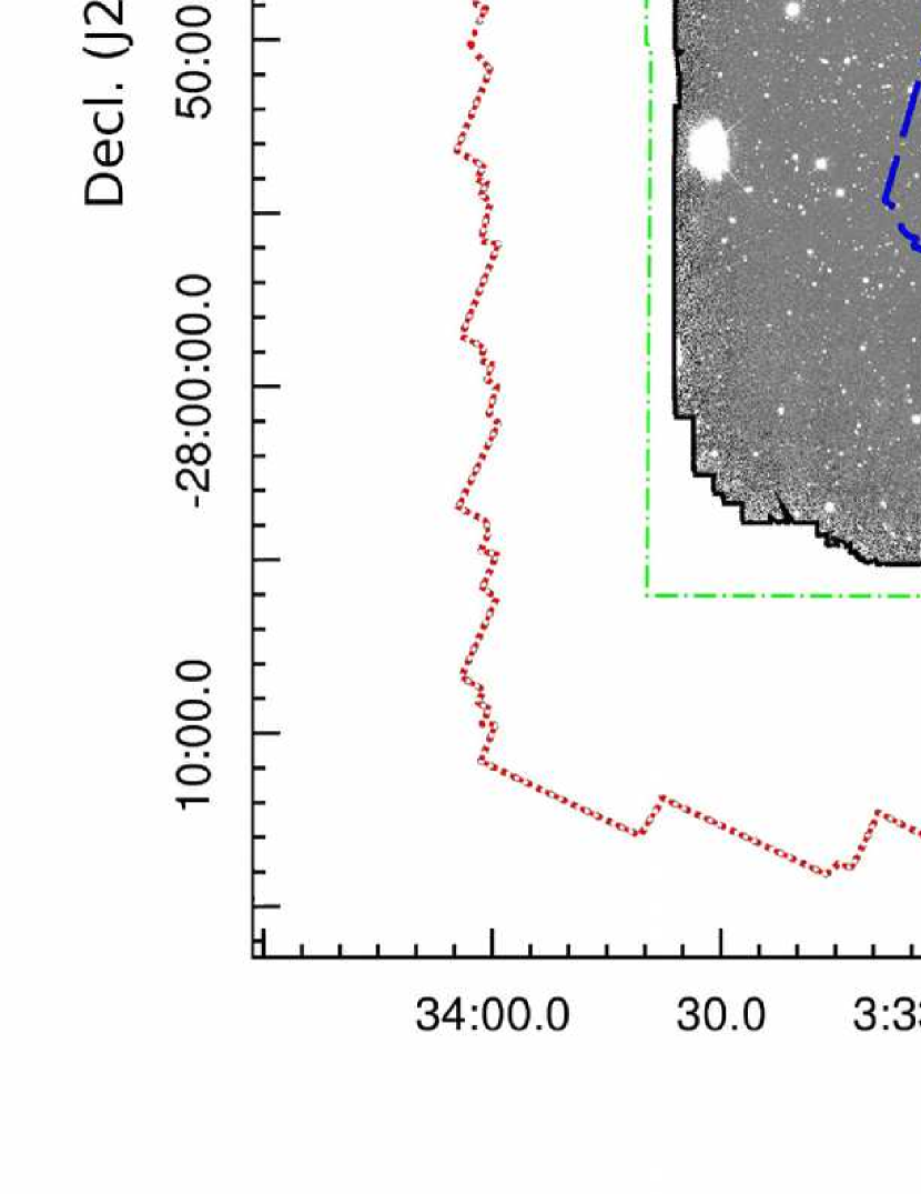
Figure 1.— The TENIS $J$+$K_{S}$ image is in grayscale. The green dot-dashed line indicates the ECDFS field, the red dotted line indicates the field of the SIMPLE data, and the blue dashed line indicates the field of the GOODS-S IRAC data.

We present the survey fields of the TENIS, SIMPLE, and GOODS-S IRAC projects in Figure 1. We describe the observations of TENIS in Section 2, the procedure of the TENIS data reduction in Section 3, and the evaluation of the reduction quality in Section 4. We describe the photometric catalog of TENIS $J$ and $K_{S}$ data in Section 5 and compare it with other NIR datasets in Section 6. In Section 7, we present our newly developed deconvolution technique for estimating IRAC fluxes in the ECDFS and examine the performance. The properties of the combined TENIS and IRAC catalog are discussed in Section 8. In Section 9, we summarize our results. The images and catalog from this work are available at the official TENIS website: http://www.asiaa.sinica.edu.tw/~bchsieh/TENIS/. All fluxes in this paper are $f_{\nu}$. All magnitudes are in AB system, unless noted otherwise, where an AB magnitude is defined as AB = 23.9 – 2.5log($\mu$Jy).

2. CFHT WIRCam Imaging Observations

The TENIS data were taken using WIRCam on the CFHT. WIRCam consists of four $2048\times 2048$ HAWAII2-RG detectors covering a field-of-view (FOV) of $20\arcmin\times 20\arcmin$ with a $0\farcs 3$ pixel scale. The gap between the four detectors has a width of $45\arcsec$. The exposures were dithered to recover the detector gap as well as bad pixels. We adopted the standard dither pattern provided by the CFHT, which distributes the exposures along a ring with a default radius of $1\arcmin 5$. However, we changed the radius every half semester or so, to $0.5\times$ to $1.5\times$ of its default value. This further randomizes the dither footprints and minimizes artifacts caused by flat fielding, sky subtraction, or crosstalk removal. At each dither point, we typically co-added two 50-second exposures and four 20-second exposures at $J$ and $K_{S}$, respectively. The typical number of dither points were 9 for $J$ and 11 for $K_{S}$, in a dither sequence. Therefore, after including the readout time (10 seconds), a dither sequence took around 20 minutes to complete. In our experience, the variation in sky color within such a short period is usually sufficiently small to allow for good flat fielding and sky subtraction.

The ECDFS has a half-degree size, which is larger than the $\sim 23\arcmin$–25$\arcmin$ dithered WIRCam FOV. To cover the ECDFS, we thus further offset the pointings between each dither sequence by $\pm 2\farcm 5$ along RA and Dec. In the $J$-band imaging, we offset primarily along the NE–SW direction, leaving shallower NW and SE corners. In the $K_{S}$-band imaging, we were able to cover all the four corners of the ECDFS.

The observations were carried out by the CFHT in queue mode with weather monitoring. Most of the data were taken under photometric conditions with similar seeing. The average seeing for the observations are $0\farcs 8$ and $0\farcs 7$ (FWHM) for $J$ and $K_{S}$, respectively. For the $J$-band data, we obtained 42.6 hours of on-source integration in semesters 2007B and 2008B. For the $K_{S}$-band data, we obtained 25.3 hours of integration in semesters 2009B and 2010B. In addition, a Hawaiian group led by Lennox Cowie obtained 13.7 hours of $K_{S}$ integration in semester 2010B. We include all the 39.0 hours of $K_{S}$ data here. The integration maps for the $J$ and $K_{S}$ data are shown in Figure 2, and the cumulative areas in the TENIS $J$ and $K_{S}$ images as functions of effective integration time are shown in Figure 3.

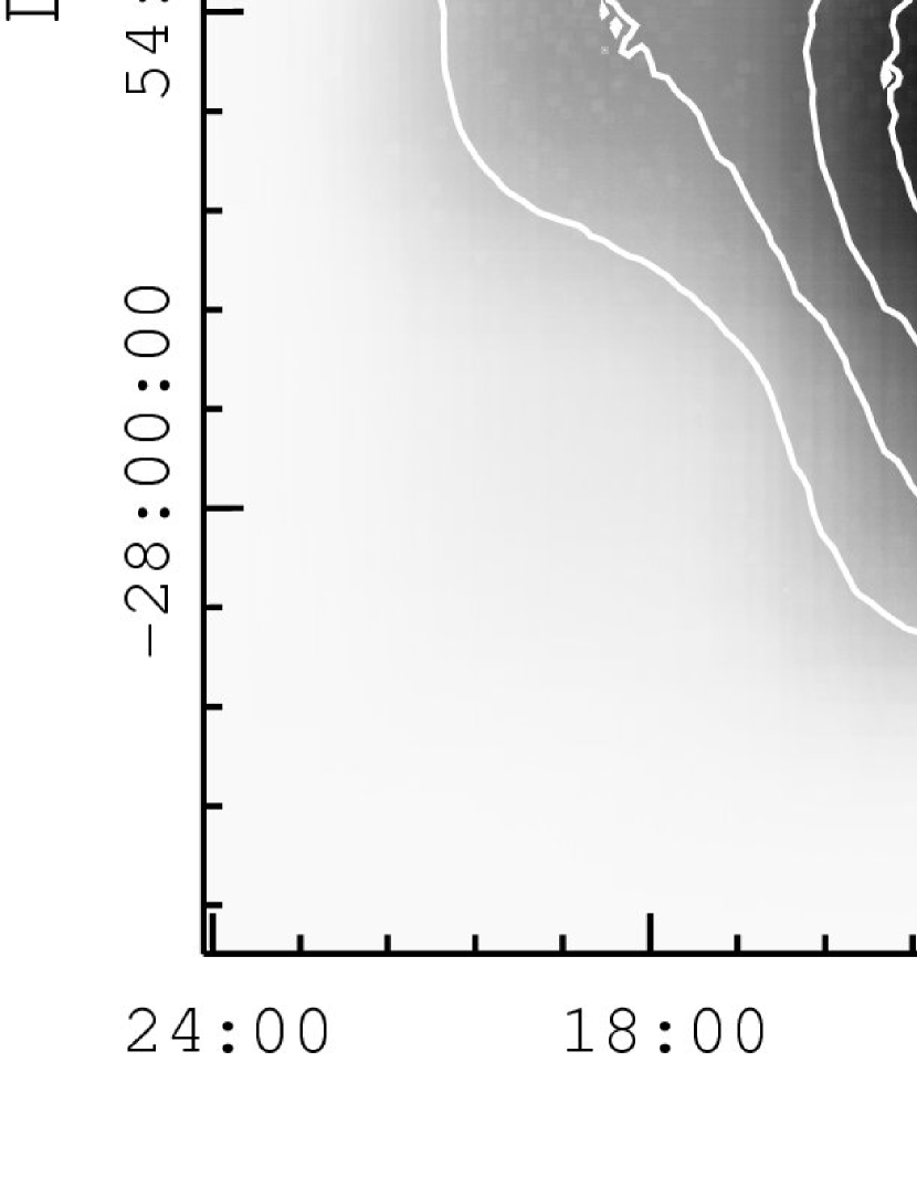
Figure 2.— Integration maps for the TENIS data. The left panel is for $J$ and the right panel is for $K_{S}$. The grayscale shows the effective integration time in each panel where darker indicates a longer integration time. The white contours indicate 20%, 40%, 60%, and 80% of the maximum effective integration time, which is 42.6 hours for $J$ and 39.0 hours for $K_{S}$.

Figure 3.— Cumulative area in the TENIS $J$ and $K_{S}$ images vs. effective integration time. The maximum effective integration time (42.6 and 39.0 hours for $J$ and $K_{S}$, respectively) is normalized to be 1.0 for each band.

3. Data Reduction

The TENIS $J$ and $K_{S}$ data were processed using an Interactive Data Language (IDL) based reduction pipeline. The details of the pipeline are described in Wang et al. (2010), who also dealt with extremely deep WIRCam imaging. The reduction here is nearly identical to that in Wang et al. (2010).

We first grouped the images and only processed images from the same dither sequence and the same detector at a time. The dithered raw images were first median-combined to produce an initial flat field. Then objects were detected on each flattened image and were masked on the associated raw image. For an image, a better flat-field image was then created by median-combining the rests of the object-masked raw images in the dither sequence. This way, every image has an associated flat field, created by avoiding itself. This is the major difference between the reduction here and that in the early data release of Wang et al. (2010). In the earlier versions of the Wang et al. (2010) pipeline, all images in a dither sequence were median combined to form a flat field image, after detected objects were masked. This produces an extremely small but statistically significant overestimate of the flat field at the locations of faint objects that are undetected in single exposures. Because the sky background is very bright, this small error in flat field translates to a larger error in the final fluxes of faint objects. This is discussed in details in the later data release of Wang et al. (http://www.asiaa.sinica.edu.tw/~whwang/goodsn_ks). We would like to draw to the community’s attention that a similar error may exist in other datasets if a similar flat-fielding method is adopted. Our reduction here avoids the above problem.

After the above flat-fielding, usually the images are sufficiently flat and only a constant background subtraction is needed. Occasional residual sky structure caused by rapidly changing sky color was further subtracted by fitting fifth-degree polynomial surfaces to the image background.

On each WIRCam detector, there is crosstalk among the 32 readout channels ($2048\times 64$ pixels each). The crosstalk has different strength within the entire detector (32 channels), and within each of the four video boards (eight channels each). For every flattened and background subtracted image, we removed the 32-channel crosstalk by subtracting the median combination of the 32 $2048\times 64$ object-masked stripes. A similar procedure is then repeated to remove the 8-channel crosstalk. This greatly suppresses the crosstalk in the images, and only very weak residual effect can be seen in the final ultradeep stack around several tens of the brightest objects in the ECDFS.

To correctly stack the dithered images, optical distortion needs to be corrected. Our reduction pipeline followed the method developed by Anderson & King (2003) to derive the distortion function. The pipeline first detected objects in all dithered images, and then calculated the spatial displacement caused by the dithering for each object. Such displacement as a function of position in the images is actually the first-order derivative of the optical distortion function. The pipeline approximated the displacement function with polynomial functions of X and Y, and integrated them back to obtain the distortion function. We referred to Wang et al. (2010) for more detailed discussion about this technique.

To obtain absolute astrometry and to project the images onto the sky, we compared the distortion-corrected object positions with the source catalog produced by the HST Galaxy Evolution from Morphology and SEDs (GEMS, Rix et al., 2004; Caldwell et al., 2008) survey. By forcing the object positions to match those in the GEMS catalog, we computed a single two-dimensional, third-degree transformation function that contains all the effects including the distortion, sky projection, and absolution astrometry, for each dithered image. Therefore, in the entire reduction, each image only underwent one geometric transform. This minimizes the impact of image smearing caused by the transform. The transformed images can then be stacked to form a deep, astrometrically correct image.

Before images were stacked, photometry is carried out on individual exposures, and compared among the exposures. This allows to adjust relative zero-points of the individual exposures. After the images in a dither sequence were stacked, absolute zero-point calibration was made by matching the fluxes in apertures of $5\arcsec$ in diameter with the “default magnitudes” in the point source catalog of the Two Micron All Sky Survey 6 (2MASS, Skrutskie et al., 2006). Since the magnitudes in the 2MASS catalog are in the Vega system, we converted the 2MASS magnitudes to fluxes based on the Vega zero-magnitudes in $J$ and $K_{S}$ of 1594 Jy and 666.8 Jy, respectively, as provided by 2MASS (Cohen et al., 2003). All the stacked, calibrated images from single-dither sequences and from the four WIRCam detectors were then mosaicked for form a wide-field, ultradeep image.

4. Reduction Quality

4.1. Astrometry

The GEMS survey used the Advanced Camera for Surveys (ACS) on the Hubble Space Telescope (HST) to image nearly the entire ECDFS. As described in the previous section, we forced our astrometry to match that of the GEMS ACS catalog. Here we compare how well our astrometry matches that of the GEMS catalog. More than 9,000 compact sources with good detections (S/N $>20$ and FWHM $<1\farcs 2$) are selected for this comparison. Figures 4 and  5 show the relative astrometric offsets between the TENIS $J$+$K_{S}$ image and the GEMS ACS catalog. As shown in Figure 4, the systematic offsets in R.A. and Decl. are $0\farcs 016$ and $0\farcs 0035$, respectively. These offsets are negligible compared with the rms scatter, which are $0\farcs 087$ and $0\farcs 080$ for R.A. and Decl., respectively. On the other hand, there are position-dependent systematic offsets. In the bottom-left panel of Figure 5, there is a wiggling structure with a scale of $\sim 0.05$ degree, which is comparable to the FOV of the ACS Wide-field Camera (WFC, Ford et al., 2003, FOV = $202^{\prime\prime}\times 202^{\prime\prime}$). Similar but less obvious structures can also be found in the other panels of Figure 5. It is highly likely that these position-dependent systematic offsets are internal to the GEMS catalog.

According to Caldwell et al. (2008), the astrometry of GEMS catalog is registered to that of the Classifying Objects through Medium-Band Observations, a spectrophotometric 17-filter survey (COMBO-17, Wolf et al., 2001). The absolute astrometric accuracy of the GEMS catalog is therefore limited by the astrometric quality of the COMBO-17 catalog, which is better than $0\farcs 15$ but which may be greater than $0\farcs 3$ in some localized regions. As we calibrated our astrometry using the GEMS catalog, the absolute astrometric accuracy of the TENIS data is therefore also limited by that of the COMBO-17 data. We could match the TENIS astrometry directly to the COMBO-17 data. However, the major scientific goal of the TENIS project is to find LBGs at $z>7$, which needs the ultra deep GEMS data. We therefore matched the TENIS astrometry to that of the GEMS data rather than that of the COMBO-17 data because it makes combining the TENIS data and the GEMS data much easier.

Figure 4.— Relative astrometric offsets between the TENIS $J$+$K_{S}$ image and the GEMS ACS catalog. We selected over 9,000 compact sources with good detections (i.e., S/N $>20$ and FWHM $<1\farcs 2$) for the comparison. The systematic offsets in R.A. and Decl. are $0\farcs 0016$ and $0\farcs 0035$, which are negligible as compared to the rms offsets, which are $0\farcs 087$ and $0\farcs 080$ for R.A. and Decl., respectively.

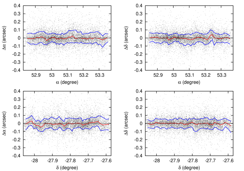
Figure 5.— Same as Figure 4 but as function of R.A. and Decl. The red line indicates the running median and the blue lines indicate the upper and lower 68th percentiles.

4.2. Photometry

As mentioned in Section 3, the TENIS WIRCam $J$ and $K_{S}$ fluxes were calibrated using $5^{\prime\prime}$ diameter apertures and matched to the fluxes in the 2MASS point source catalog. In Figure 6, we show the flux ratios between 2MASS and TENIS in $J$ and $K_{S}$, where the flux range between the two vertical dashed lines in each panel indicates that used for the calibration. Fluxes brighter than this range suffer from nonlinearity issues in WIRCam, whereas fluxes fainter than this range are subjected to selection effects due to the much shallower detection limits of 2MASS. The error-weighted means of the objects in the chosen calibration flux ranges are 1.0002$\pm$0.003 and 1.0006$\pm$0.005 for $J$ and $K_{S}$, respectively, resulting in an overall flux calibration quality that is good to 0.3% and 0.5% for $J$ and $K_{S}$, respectively. We note that the flux errors of the TENIS data are also shown horizontally in Figure 6 but are too small to be visible, and hence they make negligible contributions to the photometric error budget compared with the vertical error bars. The flux calibration quality of the TENIS data is therefore completely dominated by the 2MASS flux errors.

Figure 6.— Flux ratios between 2MASS and TENIS in $J$ and $K_{S}$. The two vertical dashed lines in each panel indicate the flux range for the flux calibration. We note that the outliers between the two vertical dashed lines are excluded in the flux calibration. The flux errors of the TENIS data are also shown horizontally but they are too small to be visible. Hence they have negligible contribution to the vertical error bars. The flux calibration quality of the TENIS data is therefore completely dominated by the 2MASS flux errors.

We also investigated the photometric uniformity in our TENIS images by subdividing the TENIS $J$ and $K_{S}$ images into four quadrants and then comparing the TENIS fluxes with the 2MASS fluxes as we did for the entire images. For quadrants 1 through 4 in $J$, the error-weighted flux ratios are 0.979 $\pm$ 0.007 (21 sources), 0.997 $\pm$ 0.006 (25 sources), 1.014 $\pm$ 0.005 (43 sources), and 1.005 $\pm$ 0.008 (22 sources), respectively. For those in $K_{S}$, they are 0.998 $\pm$ 0.009 (19 sources), 1.033 $\pm$ 0.007 (27 sources), 1.003 $\pm$ 0.009 (27 sources), 0.978 $\pm$ 0.011 (11 sources), respectively. The standard deviations of the four measured offsets are 1.3% and 2.0% for $J$ and $K_{S}$, respectively. This suggests that the photometric gradients over size scales of $\sim 15^{\prime}$ are less than 0.013 and 0.02 mag in the TENIS $J$ and $K_{S}$ images, respectively; these measured 1.3% and 2.0% are fairly good as compared to other NIR extragalactic deep surveys over similar size scales (e.g., 2% in the COSMOS survey; Capak et al., 2007).

5. The $J$ and $K_{S}$ photometric catalog

To produce a source catalog that is as complete as possible, we decide to perform object detection in a high S/N image generated by combining the TENIS $J$ and $K_{S}$ images. Such a combination has to take into account the different integration time distributions in $J$ and $K_{S}$. A straightforward method is to weight the pixels by their associated integration times and then combine the images. However, our $J$ integration time is approximately $1.32\times$ longer than the $K_{S}$ integration time, but objects are generally brighter (in our map unit, which is $\mu$Jy) at $K_{S}$. Hence, a direct integration time weighted combination is less optimal in terms of combined S/N for most objects. We therefore normalized the $J$ and $K_{S}$ integration times by artificially reducing the $J$ integration time by a factor of 1.32 (i.e., downweighting the $J$ image), and then performed the integration time weighted $J$+$K_{S}$ combination.

We used SExtractor version 2.5.0 (Bertin & Arnouts, 1996) to detect objects and measure their fluxes in the TENIS WIRCam images. The “FLUX_AUTO” values of the SExtractor output are chosen for the flux measurements. The double-image mode of SExtractor was performed to detect objects in the $J$+$K_{S}$ image while measuring fluxes in the original $J$ and $K_{S}$ images at the locations of the $J$+$K_{S}$ objects. The most important SExtractor parameters we used are listed in Table 1.

Table 1SExtractor Parameters

Parameter	Value
DETECT_MINAREA	2
DETECT_THRESH	1.3
ANALYSIS_THRESH	1.3
FILTER	Y
FILTER_NAME	gauss_2.0_3x3.conv
DEBLEND_NTHRESH	64
DEBLEND_MINCONT	0.00001
CLEAN	Y
CLEAN_PARAM	0.1
BACK_SIZE	24
BACK_FILTERSIZE	3
BACK_TYPE	AUTO
BACKPHOTO_TYPE	LOCAL
BACKPHOTO_THICK	40
WEIGHT_TYPE	MAP_WEIGHT
WEIGHT_THRESH	20

The flux errors provided by SExtractor are derived from the background noise directly, and the noise covariance between pixels (i.e., correlated error produced by image resampling, and to a lesser degree, faint undetected objects) is ignored. To mitigate against the latter effect, we calibrated the errors using the following procedure. First, the fluxes and the flux errors were re-measured using SExtractor with $2^{\prime\prime}$ diameter apertures. We then convolved the source-masked image with a $2^{\prime\prime}$ diameter circular top-hat kernel, and calculated the rms in a $10^{\prime\prime}\times 10^{\prime\prime}$ area around each pixel on the convolved image. The ratio between the aperture photometric flux error provided by SExtractor for a certain object and the rms value around the same position in the convolved image is the correction factor for its flux error. The median value of the correction factors was computed to be the general correction factor for all the sources. For the TENIS $J$- and $K_{S}$-band data, the general correction factors are very similar, which is 1.27. The same procedure was repeated with different aperture sizes. We found that the correction factors are very stable over different aperture sizes, which is consistent with the experience in Wang et al. (2010). Therefore we applied this factor to the “FLUXERR_AUTO” values for all the objects to account for the effects of noise correlation and confusion. We note that this factor does not apply to the flux measurements.

We then estimated the aperture correction for the AUTO aperture. Since we calibrated the WIRCam data to 2MASS using a $5^{\prime\prime}$ diameter aperture, we just need to derive the correction factor between the AUTO aperture and the $5^{\prime\prime}$ aperture. After comparing the fluxes derived using these two different apertures, we found that they are in very good agreement with each other for most objects. Because the photometry derived using AUTO apertures have better S/N for objects with various different morphologies and fluxes as compared to the $5^{\prime\prime}$ fluxes, we decided to use the original “FLUX_AUTO” values as the final flux measurements in our catalog.

6. Comparison with the GOODS-S/ISAAC Data

There are deep near-infrared imaging observations of the GOODS-S region using the Infrared Spectrometer And Array Camera (ISAAC) on the Very Large Telescope (VLT) in $J$, $H$, and $K_{S}$. The $K_{S}$-selected catalog is published by Retzlaff et al. (2010). According to the sensitivities provided by Retzlaff et al. (2010), the depths of the ISAAC data are comparable with that of TENIS. We have checked the photometric consistency and the data quality difference between the two catalogs. In Figure 7, we compare the TENIS $J$ and $K_{S}$ photometry with the total magnitudes in the ISAAC catalog. The ISAAC fluxes for bright stars are approximately 10% and 15% less than the TENIS fluxes at $J$ and $K_{S}$, respectively. We checked whether these large differences could be caused by the differences in the filter systems used, as shown in Figure 8. We found that the different passbands of the two filter systems can produce only $\sim 3\%$ differences in fluxes by examining the color of stars from Kurucz models (ATLAS9; Kurucz, 1993). It is also worth noting that both catalogs are not corrected for Galactic extinction, although the correction values, only 0.008 mag ($J$) and 0.003 mag ($K_{S}$), are too small to explain the $>10\%$ flux differences.

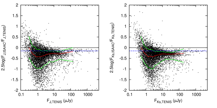
Figure 7.— Photometry comparisons between the TENIS and ISAAC catalogs. Flux ratios between the two catalogs versus the TENIS fluxes are plotted. The left panel is for $J$ and the right panel is for $K_{S}$. The red line indicates the running median and the green lines indicate the upper and lower 68th percentiles. The blue dashed line indicates a -0.15 mag difference. The results show that the ISAAC fluxes for bright stars are about 10% to 15% less than the TENIS fluxes.

Figure 8.— Transmission curves for the WIRCam and ISAAC filters. The left panel is for $J$ and the right panel is for $K_{S}$. The solid curve is for WIRCam and the dashed curve is for ISAAC in each panel.

We calibrated the TENIS photometry using the 2MASS catalog. The ISAAC observations, however, were calibrated with standard stars. We therefore directly compared the ISAAC catalog with the 2MASS catalog to see if the flux differences are due to different zeropoint calibration methods used in the two catalogs. The result is shown in Figure 9. The ISAAC total fluxes are $\sim 10$% to 15% lower than the 2MASS default fluxes, consistent with the differences between the TENIS and ISAAC fluxes. In addition, Retzlaff et al. (2010) mentioned that a significant bias ($\leq$0.1mag) is visible when comparing ISAAC to the 2MASS catalog. Hence we conclude that the flux discrepancies between the TENIS and ISAAC catalogs are due to different zeropoint calibration methods.

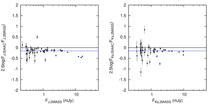
Figure 9.— Same as Figure 7 but for 2MASS and ISAAC. The blue dashed line indicates a -0.15 mag difference. The flux differences are consistent with that shown in Figure 7, which suggests that the flux discrepancies between the TENIS and ISAAC catalog are due to different zeropoint calibration methods.

To compare the depth, we plot the magnitude vs. S/N for the TENIS and ISAAC data in Figure 10. The $5\sigma$ limiting magnitudes for point sources of the ISAAC data claimed by Retzlaff et al. (2010) are about 25.0 and 24.4 for $J$ and $K_{S}$, respectively, which are consistent with what are shown in Figure 10. According to this figure, the TENIS data are about 0.5 mag deeper than the ISAAC data in both $J$ and $K_{S}$. If the abovementioned zeropoint differences are considered, the depth differences would be further increased to $>0.6$ mag. We note that the Cosmic Assembly Near-infrared Deep Extragalactic Legacy Survey (CANDELS, Grogin et al., 2011; Koekemoer et al., 2011) provides a deeper $J$-band ($F125W$) dataset in the GOODS-S region (5$\sigma$ limiting magnitudes for point sources is $\sim 27$ mag). We therefore conclude that our TENIS catalog is by far not only the deepest NIR dataset in ECDFS, but also the deepest $K_{S}$ dataset even in the narrow GOODS-S region.

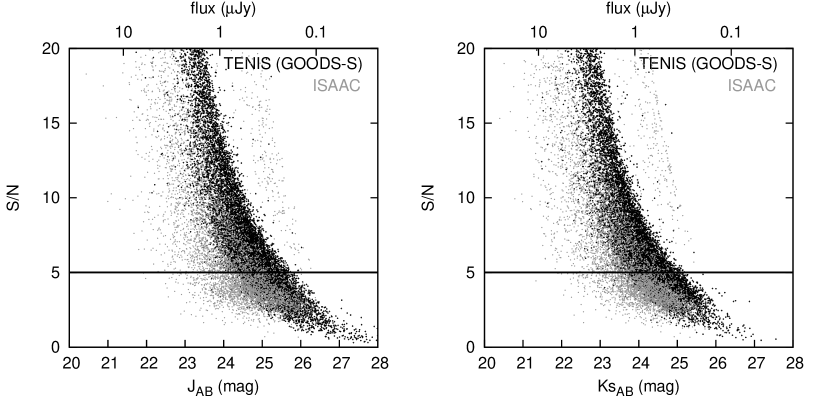
Figure 10.— S/N vs. Magnitude plots for the TENIS and ISAAC data. The left panel is for $J$ and the right panel is for $K_{S}$. The dark black dots indicate objects in the GOODS-S region in the TENIS catalog and the gray dots indicate objects in the ISAAC catalog. The horizontal line in each panel marks the S/N level of 5. Based on this comparison, the TENIS data are about 0.5mag deeper than the ISAAC data in both $J$ and $K_{S}$.

7. IRAC Photometry

The SIMPLE survey (Damen et al., 2011) provides deep IRAC observations covering the entire ECDFS with the $10\arcmin\times 15\arcmin$ ultradeep GOODS-S IRAC (M. Dickinson et al., 2012, in preparation) mosaics in its center. According to Damen et al. (2011), the $5\sigma$ limiting magnitudes for point sources typically are 23.8, 23.6, 21.9, and 21.7 for 3.6$\mu$m, 4.5$\mu$m, 5.8$\mu$m, and 8.0$\mu$m, respectively. For the ultradeep GOODS-S IRAC region, the $5\sigma$ limiting magnitudes for point sources are 26.1, 25.5, 23.5, and 23.4 for 3.6$\mu$m, 4.5$\mu$m, 5.8$\mu$m, and 8.0$\mu$m, respectively, according to Dahlen et al. (2010). As mentioned in Section 1, IRAC data are valuable for studies from Galactic objects to the high-redshift universe. Combining the SIMPLE IRAC and TENIS data can broaden the use of the TENIS catalog.

7.1. Basic Principle

The major difficulty in combining the IRAC and WIRCam data is the relatively large IRAC PSFs ($1\farcs 5$ to $2\farcs 0$) compared with of the WIRCam data ($0\farcs 8$). As a consequence, measurements of total fluxes of objects in the IRAC images require photometric apertures that are much larger than the WIRCam apertures. Given the ultradeep nature of the SIMPLE and GOODS-S IRAC images and the high surface densities of objects, large apertures mean that the photometric accuracy is highly subject to nearby bright objects as well as the large number of faint confusing sources. Because the blended objects can have very different morphology and color, accounting for this problem is crucial.

Many intensive efforts have gone into better estimating fluxes in crowded, low-resolution images. The most recent methods rely on utilizing the positional and morphological information of objects detected in a high resolution image in a different waveband (e.g., Grazian et al., 2006; Laidler et al., 2007; Wang et al., 2010; McLure et al., 2011). By assuming that the intrinsic morphology of an object is identical in the two wavebands (i.e., no color gradient from center to edge) and taking into account differences in the PSFs, one can model how an object would look like in the low resolution image based on its observed morphology in the high resolution image. Using a minimum $\chi^{2}$ method, Grazian et al. (2006) and Laidler et al. (2007) were able to model all blended objects simultaneously and thus estimate their fluxes in the low resolution image. Instead of minimizing $\chi^{2}$, another approach is to minimize residual fluxes between the model and the observed low resolution image (Wang et al., 2010). This is the basic idea of CLEAN deconvolution in radio imaging (Högbom et al., 1974).

In this work, we follow the CLEAN approach of Wang et al. (2010). However, we greatly relax the assumption on object morphology. In Wang et al. (2010), a model of the IRAC image of a galaxy is generated based on the PSFs and its high-resolution WIRCam image, and the model is then iteratively subtracted (“CLEANed”) from the real IRAC image. Here, we directly CLEAN the IRAC image of a WIRCam detected galaxy using the IRAC PSF, and we allow the cleaning position to move around its WIRCam position. In other words, our method is essentially the same as CLEAN deconvolution in radio imaging, with nearly no restrictions except for the locations where CLEAN can happen. We named this method “IRACLEAN” because it is designed for estimating IRAC fluxes.

7.2. Methodology

7.2.1 PSF Construction

The IRAC PSFs were generated using bright isolated point sources in each IRAC channel. The size of the PSF images is $1^{\prime}\times 1^{\prime}$ in order to cover the outer structure of the extended IRAC PSFs, especially for 8.0$\mu$m. To avoid saturated sources, we chose intermediate brightness objects and checked their images carefully. We also checked their optical counterparts in the extremely high resolution HST ACS images to make sure that they are really point-like. The final PSF is constructed by calculating the flux weighted mean of the PSFs of these objects with a $3\sigma$ clip. There are, however, still many objects within $1\arcmin\times 1\arcmin$ around these sources even if they are relatively “isolated”. This biases the wing of the constructed PSF. We therefore ran SExtractor on the IRAC images to generate object masks and then masked all the nearby objects when generating the PSFs. This masking procedure, however, may create many “holes” in the constructed PSF image. To overcome this, sometimes more than 20 objects have to be used for constructing one PSF. The PSFs of stars in the native IRAC images would be under-sampled because of the relatively large pixel size of IRAC ($1\farcs 2$ per pixel for the IRAC PSFs with FWHMs of $1\farcs 66$ to $1\farcs 98$). Without doing a sub-pixel centering, the constructed PSF may be artificially broadened. Since the SIMPLE image has been resampled to match the TENIS image ($\sim 0\farcs 3$ per pixel), simply finding the location of a peak is very similar to do a sub-pixel centering, and the centering accuracy of the constructed PSF is better than 9% to 7.6% ($\pm 0\farcs 15$, from 3.6$\mu$m to 8.0$\mu$m) of the IRAC FWHMs. Hence the broadening effect of the stacked PSF is negligible. We note that the PSFs in the SIMPLE images are position-dependent, and the procedure that we used to deal with this issue is described in Section 7.2.5.

7.2.2 Object Identification

We used the TENIS $J$+$K_{S}$ image as a prior to estimate the IRAC fluxes around the locations of $J$+$K_{S}$ detected objects. The location information is contained in the SExtractor “segmentation map” of the TENIS $J$+$K_{S}$ image. The segmentation map tells which detected object (or no object) a pixel is associated with. For a given $J$+$K_{S}$ detected object, we only clean its IRAC fluxes at its associated segmentation map pixels. Therefore, the boundary of an object defined in the segmentation map is equivalent to “CLEAN window” in radio imaging. In addition, since we allow any pixels within the boundary of an object to be CLEANed, we do not assume any morphology for that object except for its outer extent as defined by the $J$+$K_{S}$ image. This has the advantage of allowing changes in morphology at different wavelengths. We should note that changing the SExtractor detection threshold setting for the $J$+$K_{S}$ image (i.e., DETECT_THRESH) would enlarge and shrink the segmentation area, which might affect the IRACLEAN performance. To ensure IRACLEAN working properly, the detection threshold should be set as low as possible. Lowering the detection threshold down too much, however, would also increase the spurious rate significantly. We found that the IRACLEAN fluxes with different DETECT_THRESH values agree with each other within 3% as long as DETECT_THRESH $\leq$ 1.5, and the spurious rate increases dramatically with DETECT_THRESH $\leq$ 1.2 (see Section 8.2 for details about spurious rate). Setting DETECT_THRESH = 1.3 (see Table 1) is a good balance between IRACLEAN performance, source completeness, and spurious rate.

7.2.3 IRACLEANing Objects

We first made mosaics of the IRAC images and resampled them to match the pixel size of the TENIS $J$+$K_{S}$ image ($0\farcs 3$). The IRACLEAN process always starts at an IRAC pixel with the highest “absolute” value (i.e., the value can be negative) measured within a $9\times 9$-pixel box ($F_{AP9}$, hereafter), and this pixel ($P_{decon}$, hereafter) must have been registered to one object in the $J$+$K_{S}$ segmentation map. We chose a $9\times 9$-pixel ($2\farcs 7\times 2\farcs 7$) box as the aperture size because it delivers the best S/N. Since the IRAC image ($0\farcs 6$ per pixel) has been resampled to match the TENIS $J$+$K_{S}$ image ($0\farcs 3$ per pixel), simply moving a window (i.e., $F_{AP9}$) across the IRAC image to find the location of a peak is very similar to doing a sub-pixel centering. Once $P_{decon}$ is found, we subtracted a scaled PSF from the surrounding $1^{\prime}\times 1^{\prime}$ area centered on $P_{decon}$. The percentage of the subtracted flux (“CLEAN gain”) depends on $F_{AP9}$; if $F_{AP9}$ is greater than $20\sigma$ , then 1% of the flux was subtracted; if $F_{AP9}$ is less than $20\sigma$ but greater than $5\sigma$, then 10% of the flux was subtracted; if $F_{AP9}$ is less than $5\sigma$, then 100% of the flux was subtracted. Our gain for brighter peaks (1% for $20\sigma$) is much smaller than the values in most radio CLEAN (10%). We found a gain of 10% for saturated or extended bright sources sometimes produces unreliable results. This is likely because the IRAC PSF is not as well determined as the synthesized beam in radio imaging, so that over- or under-subtraction easily occurs. We found that a gain of 1% produces a good balance between processing speed and deconvolution quality. The subtracted flux ($F_{SUB}$) was summed and registered to the associated object in the $J$+$K_{S}$ segmentation map. After each subtraction, the IRACLEAN process is repeated on the subtracted image, until there were no pixels with $F_{AP9}$ higher than $2\sigma$. This threshold is chosen such that it is not too low to allow for unreliable objects entering IRACLEAN, and it is not too high to cut off too much useful information on weak objects. We emphasize again that the concept of the deconvolution here is identical to that of CLEAN in radio imaging.

Under some extreme conditions (unmatched PSF with saturated or bright extended objects), gains of $<1\%$ still do not work. The residual fluxes of these objects would start to oscillate and diverge with the progress of IRACLEAN, and this phenomenon usually happens when the residual fluxes are about 30% to 50% of the original fluxes. Since the PSF area we used is $1^{\prime}\times 1^{\prime}$, this effect would also seriously affect the IRACLEAN results of other objects within the $1\arcmin$ area. The IRACLEAN process will set a gain of 100% to subtract the fluxes for such objects when the signs of flux divergence show up, and then stop to clean them hereafter. It is worth noting that since greater than 50% of the flux is still cleaned by the normal IRACLEAN procedure, the bias effect of assigning a gain of 100% to the residual fluxes should be much less than 50% (i.e., $\ll$0.5 mag).

7.2.4 Flux and Error Measurements

At the end of the IRACLEAN process, the summation of $F_{SUB}$ for each object is the flux measurement of that object, and the final subtracted image is the residual map. If an object cannot be detected in IRAC images (i.e., its $F_{AP9}$ is lower than $2\sigma$), 0.0 is assigned to its flux measurement. The residual map allows us to check the quality of IRACLEAN, and is also used for estimating flux errors. The flux error of each object was calculated based on the fluctuations in the local area around that object in the residual map. Any imperfection of the PSF would cause larger fluctuations in the residual map, and this effect is included in the flux error calculation.

To estimate the flux error of an object, we convolved the residual map with a $9\times 9$-pixel top-hat kernel and then generated a noise map by calculating the rms around each pixel on the convolved residual map. In conventional aperture photometry, the flux error scales with the square-root of the aperture area. To follow this rule, we thus defined an effective aperture size for each object using the following method. First, if the IRACLEAN process always deconvolves an object at the same $P_{decon}$ (i.e., deconvolving a bright point source with a matched PSF), then the effective aperture size for this object is 81 pixels ($9\times 9$, Figure 11a). If the IRACLEAN process deconvolves a slightly extended object on two adjcent $P_{decon}$, then the effective aperture size for this object can be 90 pixels (Figure 11b), or 98 pixels (Figure 11c). For a more extended source, the distribution of these $P_{decon}$ can be more complicated, and the shape of the aperture can be irregular (Figure 11d).

Once the effective aperture size is determined, the flux error can be estimated with

$$F_{err}=\sqrt{\frac{N_{pixel}}{81}}\times\frac{\sum\limits_{i=1}^{n}rms_{i}}{n},$$ (1)

where $N_{pixel}$ is the total number of pixels in the effective aperture, $n$ is the total number of $P_{decon}$, and $rms_{i}$ is the value from the noise map for a certain $P_{decon}$. The first term in Equation 1 is to scale the flux error with the effective aperture size, and the second term is the average flux error for the local area around this object. One can use a more complicated method of calculating the second term by compute the local flux errors using different weightings. For simplicity, we just use an unweighted mean, which is similar to that used in conventional aperture photometry (cf., e.g., photometry with PSF fitting). Using Equation 1, we are able to reasonably estimate the flux error for all objects regardless of their morphologies. For an object undetected in an IRAC image, we used the coordinate of that object derived from the $J$+$K_{S}$ image, and calculated its flux error as if it was a point source (i.e., Using Equation 1 with $N_{pixel}$ = 81, $n$ = 1, $rms$ = the value from the noise map for the $P_{decon}$, where the $P_{decon}$ is the object coordinate in the $J$+$K_{S}$ image provided by SExtractor).

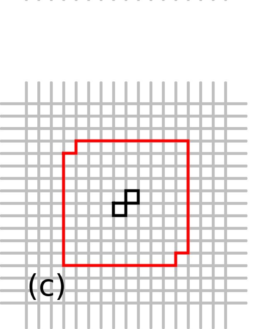
Figure 11.— Examples for calculating aperture sizes for various cases. The grid in grayscale indicates the pixels in the resampled IRAC images; the pixel marked with black color indicates $P_{decon}$; and the area marked with red color shows the aperture size for this object. Four different cases are shown in this plot: (a) a bright point source (only one $P_{decon}$ in the object center): the aperture shape is a $9\times 9$-pixel box, i.e., the total number of pixels in the aperture is 81. (b) a slightly extended source (two nearby $P_{decon}$s around the object center): the aperture shape is a $9\times 10$-pixel rectangular, and the total number of pixels in the aperture is 90. (c) a slightly extended source with different position angle as compared to case (b): the aperture size is 98 pixels. (d) an extended source: the aperture shape is more irregular and the aperture size is 140 pixels.

Since we used a $9\times 9$-pixel box as the flux aperture for IRACLEAN, an aperture correction needs to be applied for the flux errors. The value of aperture correction is derived from the deconvolution PSF for each channel. We describe the aperture correction values in Section 7.2.5.

7.2.5 Position-Dependent PSF

The PSFs in the ECDFS IRAC images change with position. This is mainly caused by the change in the orientation of Spitzer during the observations. In the GOODS-S area, the upper and lower half fields were observed with IRAC in two different epochs, with some overlap in the middle. The orientation of $Spitzer$ changed by nearly 180 degrees between the two epochs. The SIMPLE data were also taken in two different epochs with a several-degree difference in $Spitzer$’s orientation. More than $80\%$ of the SIMPLE area is covered by both epochs. In addition, there is also some overlap between the GOODS-S and SIMPLE observations. Because of the asymmetric IRAC PSFs and different orientations of $Spitzer$ in the various observing epochs, the stacked IRAC image has several different synthesis PSFs. Using a single PSF to clean the entire image will significantly degrade the IRACLEAN quality because the performance of IRACLEAN critically depends on the accuracy of the deconvolution PSF. IRACLEAN is affected by the accuracy of the deconvolution PSF in two aspects: (a) For a bright point source, using an inaccurate PSF would lead to distorted intermediate residual images after iterating the clean process many times. From this point, the local brightest pixel (i.e., $P_{decon}$) may not be around the center of this object so that IRACLEAN starts treating it as an extended source until the end of the clean process. This effect would lead to a biased flux measurement. Same thing would happen to bright extended sources, too. Fainter sources are not affected by this effect because their corresponding segmentation areas are only a few pixels hence their $P_{decon}$ pixels cannot go too far from the object centers. (b) Some fainter sources are, however, affected by another issue because of using an inaccurate PSF. If they are close to another objects that are not cleaned using accurate PSFs, then the dirty residuals of the wings of their close neighbors would contanminate their flux measurements. The brighter the close neighbor is, the more serious the effect is; the closer the separation is, the more serious the effect is. In order to obtain better flux measurements for all objects, we used several different PSFs to clean one IRAC image.

It is possible to construct many different PSFs in an IRAC image. We start with as many as seven different PSFs but below we will demonstrate that only four PSFs are necessary for 3.6 and 4.5 $\mu$m. First, we generated seven PSFs by picking up bright point-like sources from seven different areas in the IRAC image for each IRAC band. The generated PSFs are shown in Figure 12. Then for a given IRAC band, we repeated the IRACLEAN process seven times using one of the seven PSFs each time. This gives seven flux measurements for each object. Since our flux errors (Section 7.2.4) contain the effect of unmatched PSF, we can use the flux errors as an indicator on which PSF works the best on each object.

Figures 13 and 14 compare the flux errors based on the seven PSFs at 3.6 and 4.5 $\mu$m, respectively. In the $i$-th column, we pick up objects whose flux errors are the lowest when IRACLEANed with the $i$-th PSF. Then in the $j$-th row, we compare their flux errors based on the $j$-th PSF with respect to the flux errors based on the $i$-th (best) PSF. The x-axis in each panel is object ID and the y-axis is the error ratio of $j$-th to $i$-th PSF. (Since in each panel we are always comparing against the best PSF, the flux ratios in all the panels are always greater than 1.) In other words, the comparison shows how the other PSFs perform when compared to the best-matched PSF for each object.

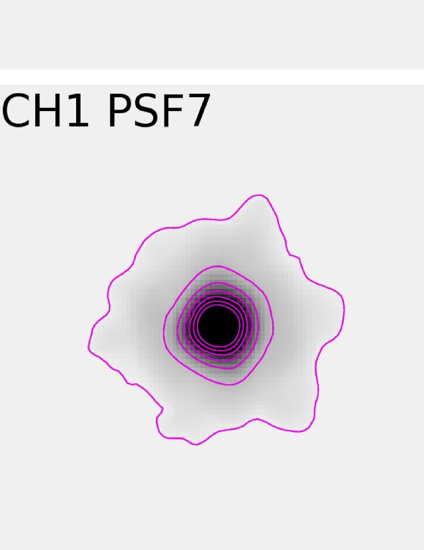
Figure 12.— The PSF images for IRAC 3.6$\mu$m to 8.0$\mu$m. The image size is $1^{\prime}\times 1^{\prime}$ in each panel. There are seven testing PSFs for 3.6$\mu$m and for 4.5$\mu$m, and one PSF for 5.8$\mu$m and 8.0$\mu$m. Contours are plotted on the PSF images for IRAC 3.6$\mu$m and 4.5$\mu$m to make the differences between PSFs visually clearer.

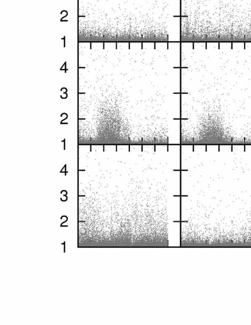
Figure 13.— Comparison of the performance of the seven PSFs at 3.6 $\mu$m. The $i$-th column contains objects whose flux errors are the lowest when IRACLEANed with the $i$-th PSF. The $j$-th row compares the errors derived with the $j$-th PSF against the errors with the $i$-th (best) PSF. X-axis is object ID and Y-axis is error ratio in each panel. See text for details.

Figure 14.— Same as Figure 13 but for 4.5$\mu$m.

By examining Figures 13 and 14, we can determine which PSF is necessary and which PSF is redundant. In a panel, if most of the error ratios are fairly close to 1, it means that the IRACLEAN results using the $i$-th PSF and the $j$-th PSF have similar quality. In such a case, the $i$-th and $j$-th PSFs can be replaced by each other. For example, we found that for 3.6 $\mu$m, PSF5 and PSF7 can both be replaced by PSF2, and PSF1 can be replaced by any of the other PSFs. In other words, only PSF2, 3, 4, and 6 are necessary for IRACLEAN at 3.6 $\mu$m. Similarly, only PSF1, 2, 4, and 5 are necessary for 4.5 $\mu$m. For 5.8 and 8.0 $\mu$m, we do not find significant differences among the seven PSFs, so only one PSF each is adopted and is shown in Figure 12.

To show how seriously IRACLEAN is affected by the accuracy of the deconvolution PSF, we calculated the rms scatters of the IRACLEAN measurements using the seven different PSFs for all the objects in 3.6 $\mu$m and 4.5 $\mu$m, and compared them with the noises measured from the residual images. The results are shown in Figure 15. According to Figure 15, the IRACLEAN fluxes of the bright isolated objects are affected by PSF more seriously than that of the faint isolated objects, which can be explained by the abovementioned effect (a). Most of non-isolated objects are faint objects since bright objects have lower surface number density hence they are more isolated. These non-isolated faint objects show another distribution in this plot. Many of them are also seriously affected by inaccurate PSF, which can be explained by the abovementioned effect (b). Figure 14 proves that the performance of IRACLEAN critically depends on the PSF, and using multiple PSFs to clean the IRAC 3.6 $\mu$m and 4.5 $\mu$m images can gain the most advantage from IRACLEAN.

Figure 15.— IRACLEAN performance affected by the accuracy of the deconvolution PSF. The left panel is for IRAC 3.6 $\mu$m and the right panel is for IRAC 4.5 $\mu$m. The Y-axis is the ratio between the scatter of fluxes measured using different PSFs and the residual noise. The X-axis is the IRAC flux measured using the best PSF. The black solid line indicates a ratio of 1.0 for Y-axis The higher the flux rms to noise ratio is, the more serious the PSF effect is. The light grey data points indicate isolated objects defined as that they have no neighbors brighter than 30% of their fluxes within $6\farcs 0$. The dark grey data points are the rest of objects. The ratio between the numbers of isolated and non-isolated objects is about 2:5. The IRACLEAN fluxes of the isolated and non-isolated objects can be affected by the accuracy of the deconvolution PSF because of different reasons. See text for details.

With the above experiments, we adopted the IRACLEAN results based on the final four PSFs for 3.6 and 4.5 $\mu$m, and one PSF each for 5.8 and 8.0 $\mu$m. For a given object, we pick the flux measurement with the lowest error among the four PSFs at 3.6 and 4.5 $\mu$m. We then calculated the aperture correction factors for each channel based on the PSFs. For 3.6 $\mu$m and 4.5 $\mu$m, the correction factors derived from the four PSFs agree with each other within 1% and we adopted the mean values. It is worth noting that the correction factors from different PSFs are very similar because these PSFs are synthesized from the same PSF with different orientations, hence the ratios of fluxes between inside and outside the aperture for different PSFs agree with each other very well. It also suggests that the centering issue of generating the stacking PSFs is negligible. The adopted aperture correction factors are 1.894, 1.875, 2.111, and 2.334 for 3.6, 4.5, 5.8, and 8.0 $\mu$m, respectively, for our $2\farcs 7\times 2\farcs 7$ flux aperture.

7.2.6 Known Issues

Three extremely bright (thus saturated) stars and several very bright objects are in the ECDFS. They have very bright wings and occupy areas that are much broader than $1^{\prime}\times 1^{\prime}$ (the deconvolution PSF size). Objects close to these bright sources, including those around the diffraction spikes and crosstalk features, therefore have higher flux measurements. In addition, as mentioned in Section 7.2.3, we stop the IRACLEAN process if it starts diverging for some bright objects. This also implies that the flux measurements of nearby objects are affected. However, we should note that the flux measurements of these nearby objects will be affected even more seriously if we do not stop the IRACLEAN process when divergence happens.

7.3. Quality and Performance

7.3.1 Residual Images

We demonstrate the performance of IRACLEAN in Figure 16. Regions of sizes $300^{\prime\prime}\times 140^{\prime\prime}$ in the SIMPLE IRAC images (left panels) and their residual images (right panels) are shown. All images are shown with inverted linear scales. The brightness and contrast of each panel are identical. By visually checking the residual images, we found that IRACLEAN works reasonably well in all four channels. For 3.6$\mu$m and 4.5$\mu$m, however, there are halos around many sources in the residual images, which may be due to unmatched deconvolution PSFs and/or under-sampled PSF caused by the large pixel scale of IRAC. The 3.6 $\mu$m or 4.5 $\mu$m residual images shown in Figure 16 are generated using a single deconvolution PSF. However, as discussed in Section 7.2.5, there are indeed four PSFs for each band, and thus three more versions of residual images each, which are not shown here. Since we adopt the result that has the lowest residual fluctuation for each object, the IRAC fluxes for 3.6$\mu$m and 4.5$\mu$m in our photometric catalog are indeed better than the visual impression based on any single residual image. On the other hand, for 5.8$\mu$m and 8.0$\mu$m, the residual maps are very clean; there are no obvious residual effects or artifacts.

Figure 16.— Performance of IRACLEAN. The SIMPLE IRAC images are shown in the left panels and their residual images are in the right panels. The region in each panel is $300^{\prime\prime}\times 140^{\prime\prime}$. North is up and east is to the left. The brightness and contrast of each panel are identical. From top are the IRAC images of 3.6$\mu$m (channel 1) to 8.0$\mu$m (channel 4). All images are shown with inverted linear scales.

7.3.2 Monte-Carlo simulations

To further understand the performance of IRACLEAN, we carried out simple Monte-Carlo simulations for objects with high S/N (S/N$\sim 50$) blended by nearby objects. All the simulated objects have flat spectra and are point-like. The separations between the blended objects are from $1\farcs 2$ to $3\farcs 9$ and the flux ratios between the blended objects are from 1 to 100. We simulated a $J$+$K_{S}$ image of the blended objects and corresponding images for four IRAC channels. The PSF of the $J$+$K_{S}$ image is extracted from the real $J$+$K_{S}$ data. The PSF for each object in the simulated $3.6\mu$m and $4.5\mu$m images is randomly picked up from the seven PSFs described in Section 7.2.5 and in Figure 12. We ran SExtractor on the simulated $J$+$K_{S}$ images to generate the segmentation map, and then performed IRACLEAN on the simulated IRAC images. We adopted only four PSFs for IRACLEAN for 3.6$\mu$m and for 4.5$\mu$m, as in our real IRACLEAN (see Section 7.2.5).

Figure 17 shows the results of the Monte-Carlo simulations. For all pairs with flux ratios $>40$ and some pairs with separations $<2\farcs 5$, SExtractor cannot resolve them in the simulated $J$+$K_{S}$ image. On such cases, IRACLEAN does not know there exist two objects, and thus we have no handle on them. These cases are not shown in Figure 17. This is a limit of the WIRCam imaging, not IRACLEAN. On the other hand, when SExtractor is able to resolve the objects, IRACLEAN has very good performance for blended objects with separations greater than $3\farcs 0$ within the entire flux ratio range. For the fainter objects in pairs, the fluxes can be under-estimated by up to 50% with separations less than $3\farcs 0$; the smaller the separation, the more severe the under-estimate is, and it is flux ratio dependent. For the bright objects in pairs, however, the fluxes can be over-estimated by up to 50% with separations less than $2\farcs 0$ when flux ratios are less than 3.5. In these extreme cases, we are pushing both IRACLEAN and SExtractor to their limits.

To estimate how many sources in our catalog may suffer from the under-estimate issue of the fainter source in a pair, we used the results of the Monte-Carlo simulations to determine the flux ratio ($FR$) vs. angular separation relation where the flux is under-estimated by 20%, and the relation can be described by

$$AS=1.84+0.5\times log(FR),$$ (2)

where $AS$ is the angular separation and $FR$ is the flux ratio. In other words, if one pair with a flux ratio of $FR$ has an angular separation less than $AS$, the flux of the fainter object in the pair is under-estimated by greater than 20% (but not by $\gg$50% according to our simulations). We then used Equation 2 to estimate how many sources in our catalog are in the abovementioned situation. The numbers are 3347 (5.4%), 2840 (4.6%), 1086 (1.7%), and 691 (1.1%) for 3.6$\mu$m, 4.5$\mu$m, 5.8$\mu$m, and 8.0$\mu$m, respectively. Fewer sources are effected in 5.8$\mu$m and 8.0$\mu$m because of their much lower surface number densities due to the shallower detection limits (see Section 8.1 for details).

To estimate how many sources in our catalog may suffer from the over-estimate issue of the brighter object in a pair, we utilized Equation 2 with $FR\leq 3.5$ to repeat the counting but for the brighter sources. The numbers are 872 (1.4%), 707 (1.1%), 430 (0.7%), and 272 (0.4%) for 3.6$\mu$m, 4.5$\mu$m, 5.8$\mu$m, and 8.0$\mu$m, respectively. It is worth noting that the real number of objects which are affected by the under-estimate and over-estimate issues may be less than the abovementioned estimated number because the $FR$s calculated using the fluxes of real objects in our catalog are already biased by the under-estimate and over-estimate issues so that the resulting $AS$’ from Equation 2 are greater than the ideal one calculated using the unbiased fluxes.

Figure 17.— Simple Monte-Carlo simulations of IRACLEAN for two blended objects. The simulation includes different angular separations and flux ratios between two blended objects. Four large panels indicate the simulation results for four IRAC channels. The FR value shown in each sub-panel is the flux ratio between two blended objects. The ratios between the output flux and the input flux of objects in the blended pairs are shown in the vertical axes. The open box indicates the brighter object in a pair while the filled box indicates the fainter one. Some missing filled boxes in each panel mean that SExtractor cannot successfully deblend the two objects in the WIRCam image; IRACLEAN is not able to handle this case since it relies on SExtractor for object detections. The IRACLEAN fluxes of the brighter objects in pairs therefore are the combined fluxes of both objects in pairs.

These results suggest that the performance of IRACLEAN is generally good and only a small number of objects in our catalog are affected by their neighbors, and the effect is not $\gg$50%. This simple simulations, however, do not include different morphologies, number of blended objects, and S/N ratios. We therefore perform another simulation using the mock IRAC images to take the abovementioned parameters into account, and show the results in Section 7.3.3.

7.3.3 Mock IRAC image simulations

To evaluate the IRACLEAN performance affected by the effects of morphology, number of blended objects, and S/N ratio, We generated four mock IRAC images by convolving the $J$+$K_{S}$ mosaic with the ideal IRAC PSFs for the four IRAC channels. We then ran IRACLEAN on these mock IRAC images with the segmentation map of the original $J$+$K_{S}$ image. Assuming the SExtractor FLUX_AUTO measurement of each object in the original $J$+$K_{S}$ image is the true flux amplitude , we can examine how well IRACLEAN performs under a complicated condition by checking if IRACLEAN can recover the SExtractor fluxes. The results are shown in Figure 18. For 3.6 $\mu$m and 4.5 $\mu$m, the fluxes in general are not under-estimated according to their running medians. For 5.8 $\mu$m and 8.0 $\mu$m, however, the fluxes around 3.0 are under-estimated by 0.05 to 0.1 mag in general because of their larger PSFs. We should note that for the real SIMPLE IRAC data, the depths in 5.8 $\mu$m and 8.0 $\mu$m are much shallower than that in $J$, $K_{S}$, 3.6 $\mu$m, and 4.5 $\mu$m, so the surface number densities in 5.8 $\mu$m and 8.0 $\mu$m are much lower than that in the other bands. The under-estimated issue for 5.8 $\mu$m and 8.0 $\mu$m shown in our simulations should therefore be much milder in the real SIMPLE data. For fluxes fainter than 2.0, they are over-estimated because of the selection effect in the fainter data. According to this plot, we conclude that the real SIMPLE IRACLEAN fluxes with greater than $5\sigma$ detections would have biases $\ll$0.1 mag.

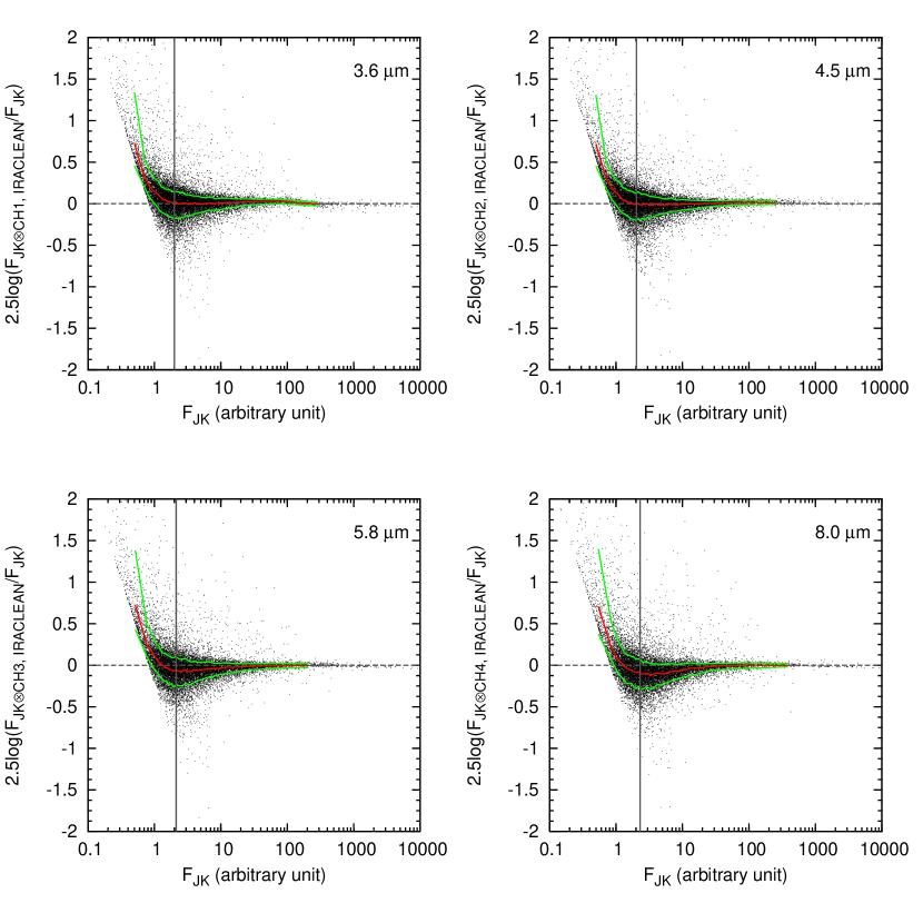
Figure 18.— IRACLEAN performance on the mock IRAC images. Four panels from left to right, top to bottom are for 3.6 $\mu$m, 4.5 $\mu$m, 5.8 $\mu$m, and 8.0 $\mu$m. The Y-axis is the magnitude difference between the IRACLEAN flux in the mock IRAC image and the SExtractor flux in the original $J$+$K_{S}$ image. The X-axis is the SExtractor flux in the original $J$+$K_{S}$ image. The red line indicates the running median while the green lines indicate the upper and lower 68th percentiles of the distribution. The vertical grey line indicates the 5$\sigma$ limit of IRACLEAN flux.

We also ran SExtractor in the single-image mode for the mock IRAC images and the results are shown in Figure 19. According to Figure 19, the under-estimate issue of SExtractor is more severe than that of IRACLEAN, and the scatters are at least a factor of 2 of that using IRACLEAN. The results suggest that IRACLEAN should perform better than SExtractor for the SIMPLE IRAC images.

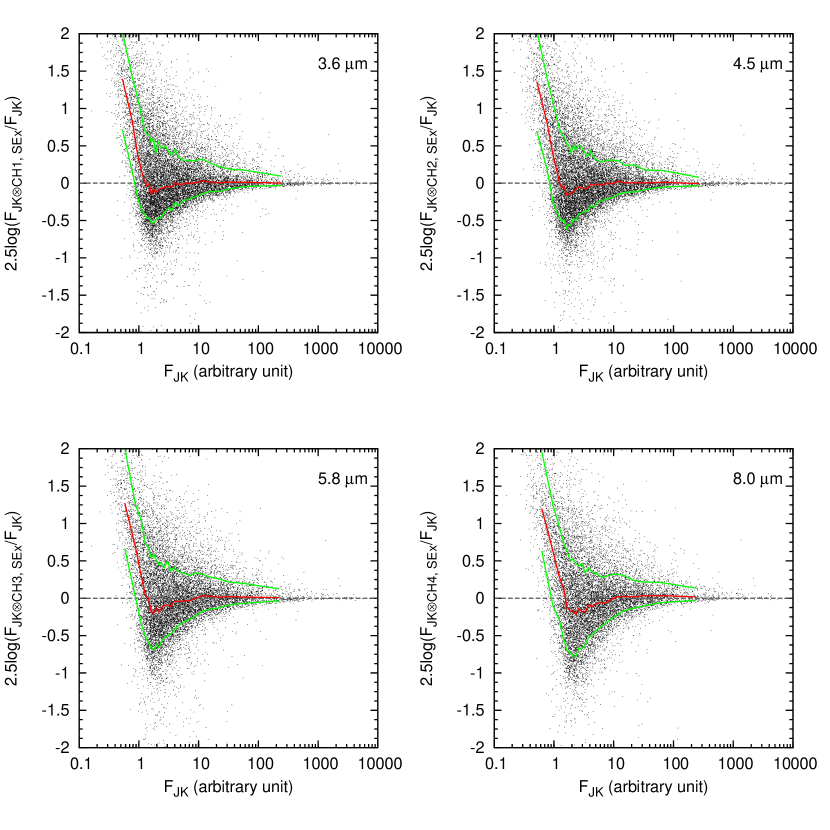
Figure 19.— Same as Figure 18 but using SExtractor.

7.3.4 Comparison with the cross-convolution method

In Wang et al. (2010), an alternative cross-convolution method (XCONV) was introduced for measuring $K_{S}$–IRAC color. The concept of this cross-convolution method is to match the PSF between $K_{S}$ and each IRAC channel by convolving their PSFs to each other. Since this method does not require any IRACLEAN procedure but just simple photometric measurements on PSF-matched images, it should provide the most accurate $K_{S}$–IRAC colors for isolated bright objects. We thus compare our IRACLEAN results with XCONV colors.

We first convolved each IRAC image with the WIRCam $K_{S}$ PSF, and convolved the WIRCam $K_{S}$ image with the IRAC PSFs we used in IRACLEAN. We take into account that there exist four different IRAC PSFs at 3.6 and 4.5 $\mu$m (Section 7.2.5). The FWHMs of the XCONVed PSFs are between $2^{\prime\prime}$ to $3^{\prime\prime}$. We then used the double-image mode of SExtractor to measure fluxes on these XCONVed images, by using the unconvolved $J$+$K_{S}$ image as the detection image. Because we focus on measuring $K_{S}$–IRAC colors here, we do not need to recover total fluxes since we have matched the PSFs in the $K_{S}$ and IRAC images. We adopt an aperture size of $3^{\prime\prime}$ in diameter in all cases, to have a good balance between S/N and the inclusion of most fluxes for all kinds of source morphologies. These are all similar to the XCONV method in Wang et al. (2010).

The comparisons of the $K_{S}$–IRAC colors derived using the IRACLEAN and XCONV methods are shown in Figure 20. The $K_{S}$–IRAC colors derived using both methods are consistent with each other. The systematic offsets between these two colors (XCONV–IRACLEAN) for 1,231 objects with $F_{Ks}>100\mu$Jy are -0.032, -0.011, -0.031, and -0.011 mag, for 3.6, 4.5, 5.8, and 8.0 $\mu$m, respectively, which are within their statistical errors. We note that in the IRACLEAN case, the $K_{S}$ fluxes are measured using the SExtractor AUTO aperture, which can miss up to 5% of total fluxes (Bertin & Arnouts, 1996). The IRACLEAN measurements of the IRAC fluxes, however, does not have such systematics. This may explain why the IRACLEAN colors are systematically redder than the XCONV colors. Nevertheless, the consistency between the two colors is fairly good. We also checked the objects with color differences greater than 0.2 mag and $F_{Ks}>100\mu$Jy. Most of them are in crowded areas with multiple bright sources so that their XCONV colors may be biased because of the large XCONV PSFs. Only a few of them are saturated/bright extended objects where their flux measurements are affected by the limitations of IRACLEAN, as we mentioned in Section 7.2.6.

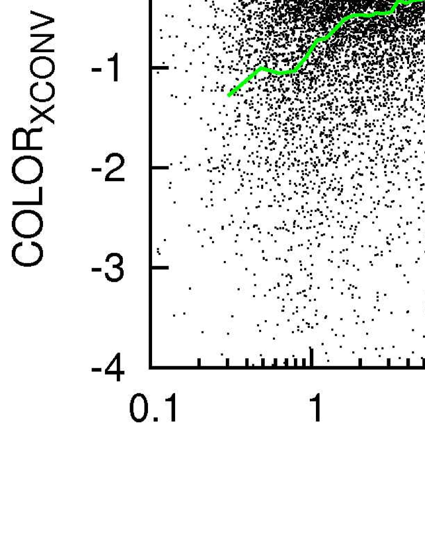
Figure 20.— Color differences between the IRACLEAN and XCONV methods. The red line indicates the running median and the green lines indicate the upper and lower 68th percentiles. The systematic offsets between these two colors for 1,231 objects with $F_{Ks}>100$ are -0.032, -0.011, -0.031, and -0.011 for 3.6$\mu$m, 4.5$\mu$m, 5.8$\mu$m, and 8.0$\mu$m, respectively. The plot shows that the $K_{S}$ - IRAC colors derived using both methods are consistent with each other.

7.3.5 Comparison with SExtractor

Figure 21 shows a comparison of IRAC photometry using IRACLEAN against that using SExtractor with FLUX_AUTO in the single-image mode. The two photometric methods are consistent on bright objects, but the scatter increases on fainter objects. Even on bright objects, as well as faint objects, there are small magnitude offsets. The gray dashed lines in the figure indicate a magnitude difference of -0.05, which well describe the differences in magnitudes derived using the two methods. This is consistent with the 5% flux loss of SExtractor FLUX_AUTO discussed in Bertin & Arnouts (1996).

At 3.6 and 4.5 $\mu$m, the distributions of flux ratios are asymmetric about -0.05 mag. There are more objects whose SExtractor fluxes are larger than IRACLEAN fluxes. This is consistent with SExtractor fluxes being boosted by nearby objects. Such a trend is not apparent at 5.8 $\mu$m and is even reversed at 8.0 $\mu$m. In these two bands, the sensitivity is lower and thus the mean separation between detected objects is larger. This makes flux booting by nearby objects less an issue. In addition, the SExtractor auto aperture may miss a great portion of the flux of faint objects given the much broader PSFs at the longer IRAC wavelengths.

Some bright sources have $>0.1$ mag differences between their IRACLEAN and SExtractor fluxes. According to the flags provided by SExtractor, more than 70% of objects brighter than 50$\mu$Jy are blended with their neighbors. In most of these cases, the SExtractor fluxes are brighter than the IRACLEAN fluxes, consistent with their SExtractor fluxes being boosted by their neighbors. In a handful of cases, the large mag differences are a consequence of terminating IRACLEAN on saturated/bright extended objects as discussed in Section 7.2.6. We also verify that all the objects with large differences between their IRACLEAN and SExtractor fluxes are blended with their neighbors. According to Section 7.3.3, IRACLEAN can provide better flux estimates for faint sources in the IRAC images, and thus the majority of scatter in Figure 21 would be due to the limitation of SExtractor.

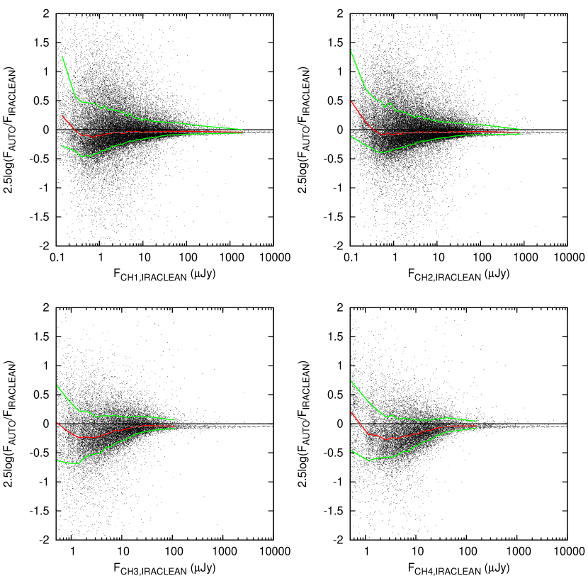
Figure 21.— The comparison of the IRAC photometry between the IRACLEAN and FLUX_AUTO methods. X-axis is the flux for each IRAC channel and Y-axis is the magnitude difference (or flux ratio) between IRACLEAN and FLUX_AUTO methods. The black line indicates 0 offset while the gray dashed line indicates an offset of -0.05 for Y-axis. The red line indicates the running median and the green lines indicate the upper and lower 68th percentiles. The offsets between the results derived using the two methods are consistent with the missing flux ratio provided by Bertin & Arnouts (1996).

7.3.6 Comparison with the FIREWORKS Catalog

We compared our IRAC fluxes with those from the FIREWORKS catalog (Wuyts et al., 2008), which provides the fluxes for the IRAC GOODS-S data. Wuyts et al. (2008) used the segmentation map generated from the VLT ISAAC $K_{S}$-band (Retzlaff et al., 2010) image as a prior and convolved the $K_{S}$-band image with IRAC PSFs for each object. They then tried to remove the neighbors around a certain object in the IRAC images, by subtracting their flux-matched convolved images. By assuming that all the neighbors are well-subtracted for the target, they then directly put an aperture to measure its flux. This is an alternative method to minimize the blending issue for IRAC flux measurements, and it is very useful to compare the relative merits of IRACLEAN and the method used by Wuyts et al. (2008).

We show the comparison in Figure 22. In general the IRAC fluxes between the two catalogs are consistent with each other. The very small dispersions in Figure 22, especially for 3.6 and 4.5 $\mu$m, imply that these two entirely independent methods both work well in terms of resolving the IRAC blending issue. There are, however, small differences between the two catalogs. At the bright end, objects brighter than 30 $\mu$Jy have $\sim 5$% higher fluxes in the FIREWORKS catalog. At the faint end, particularly at 5.8 and 8.0 $\mu$m, objects also have higher fluxes in the FIREWORKS catalog. The exact nature of these small differences are unclear to us. They are unlikely due to under-estimated IRACLEAN fluxes for blended objects, as we demonstrated in our Monte Carlo simulations (Section 7.3.2). We suspect that they are caused by the unmatched PSFs in Wuyts et al. (2008), since they did not deconvolve their $K_{S}$ image with the $K_{S}$ PSF before the convolution with the IRAC PSFs, which may lead to over-subtracting the outer wings of the neighboring objects and cause under-estimated local background. However, this is hard to verify with the data we have and without knowing the exact procedure in Wuyts et al. (2008).

Notice that the scatter in the distributions at the faint end at 3.6 and 4.5 $\mu$m in Figure 22 are very small. This suggests that the reference image (i.e., the ISAAC $K_{S}$ image) is not as deep as the IRAC 3.6 and 4.5 $\mu$m images, so the fluxes of many fainter IRAC objects were not measured and included into the FIREWORKS catalog. Moreover, the faint IRAC objects that are not detected in the ISAAC $K_{S}$ image were not subtracted before aperture photometry was applied to their brighter neighbors. Therefore, the fluxes of their brighter neighbors may be over-estimated. They may also contribute to the background noise and make the FIREWORKS detection limits worse.

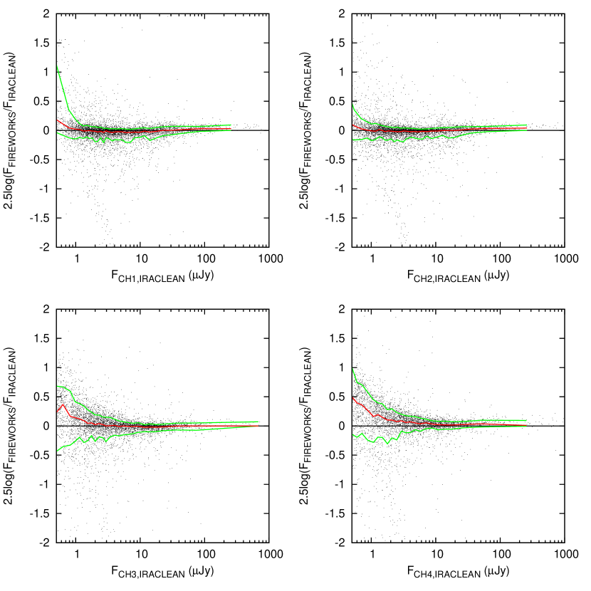
Figure 22.— IRAC photometry comparison between our catalog (IRACLEAN method) and the FIREWORKS catalog. The red line indicates the running median while the green lines indicate the upper and lower 68th percentiles. The majority of objects have similar fluxes in the two catalogs with an rms of flux ratio dispersions of less than 8%.

7.3.7 Comparison with the SIMPLE Catalog

Damen et al. (2011) published a photometric catalog of the SIMPLE data. They used AUTO aperture in SExtractor to measure fluxes of all objects. If the AUTO aperture for an object is smaller than $4^{\prime\prime}$ in diameter, they replaced the AUTO flux with flux measured with a fixed $4^{\prime\prime}$ diameter aperture. If objects are blended, their $4^{\prime\prime}$-aperture fluxes are also used. They then applied aperture corrections on all these objects. Damen et al. (2011) excluded blended objects when they compared their source fluxes with the FIREWORKS catalog, claiming that these objects worsen the comparison. We thus first compare our fluxes with the SIMPLE catalog on isolated objects according to the blended flag in the SIMPLE v3.0 catalog. The result is shown in Figure 23 and the comparison is fairly good. We emphasize, however, that more than 70% of the matched objects are marked as blended sources in the SIMPLE catalog. The result shown in Figure 23 is therefore not a representative comparison between the two catalogs.

We next compare our IRACLEAN results with the SIMPLE v3.0 catalog on blended objects. The results, shown in Figure 24, are quite striking. There are two distinct sequences in each IRAC band. The upper sequences contain approximately 66%, 68%, 54% and 51% of all blended objects at 3.6, 4.5, 5.8, and 8.0 $\mu$m, respectively. The SIMPLE fluxes of the upper sequences are only slightly higher compared with our IRACLEAN fluxes. The reason for the differences is that the SIMPLE fluxes of blended sources would be over-estimated because conventional aperture photometry method was used, while the IRACLEAN method is designed to estimate relatively unbiased fluxes for blended sources. On the other hand, the SIMPLE fluxes of the lower sequences are between 30% to 60% lower than the IRACLEAN fluxes. This very large offset, and the fact that there are two distinct sequences, cannot be explained by any systematic effects that we are aware of. We looked at the objects in the lower sequence objects in the IRAC images, but did not find anything different about these objects compared with those in the upper sequences. We remind the reader at this point that both IRACLEAN and the method used by Damen et al. (2011) to derive fluxes of indiviaul objects are based on the same SIMPLE IRAC images, yet we do not see such second sequences when we compare our results with XCONV, SExtractor, and FIREWORKS. The exhaustive comparisons that we have made with all relevant existing catalogs suggest that the lower sequences are previously unknown systematic effects in the SIMPLE v3.0 catalog. We are therefore concerned about the conclusions reached in studies that have been made based on the SIMPLE v3.0 catalog.

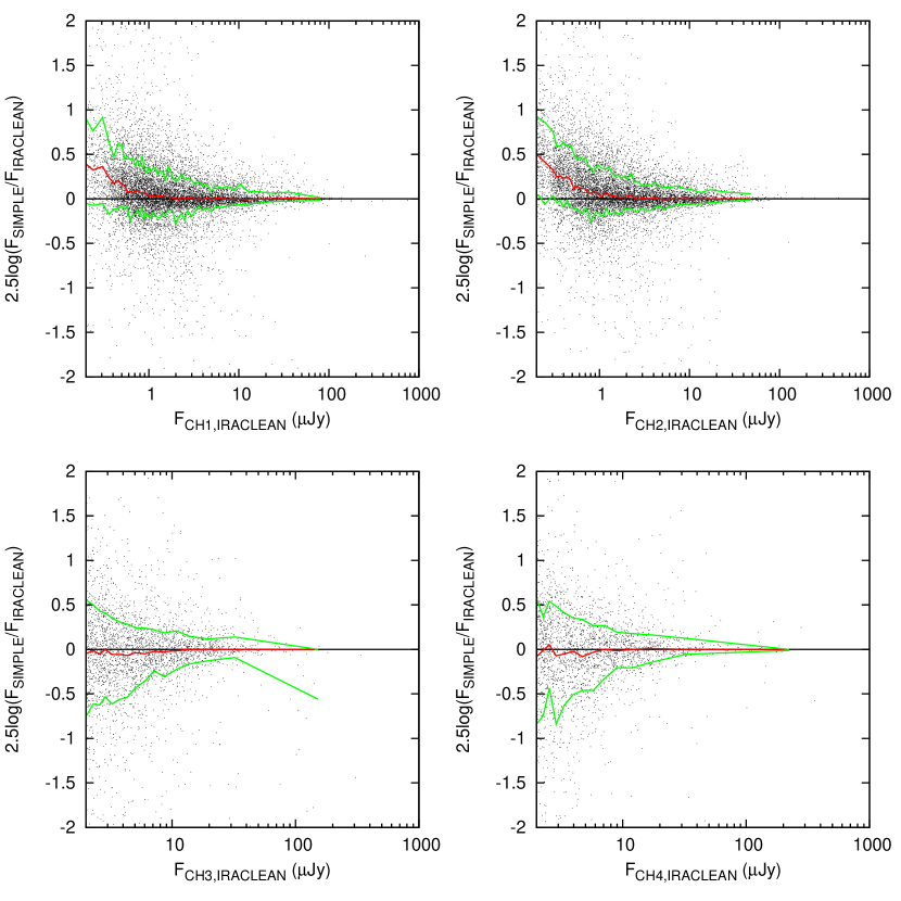
Figure 23.— Photometry comparison between the IRACLEAN flux and the SIMPLE catalog. The red line indicates the running median while the green lines indicate the upper and lower 68th percentiles. Only isolated objects are shown as suggested by Damen et al. (2011). According to this figure, the fluxes of isolated objects are consistent between both catalogs very well.

Figure 24.— Same as Figure 23 but for blended objects.

8. Combined NIR and IRAC Catalog

We combined the TENIS WIRCam photometry and the SIMPLE IRACLEAN photometry. We also removed objects with fluxes less than 3$\sigma$ in both the $J$ and $K_{S}$ bands. The final TENIS WIRCam and IRAC catalog includes 62,326 objects. We did not apply Galactic extinction correction to this catalog. We also include the XCONV colors since they are good color references for isolated bright sources. Table 2 shows the statistics of this catalog which has the following format:

$(1)$: Object ID.

$(2)-(3)$: R.A. and Decl.

$(4)-(15)$: Flux and flux error measurements (in $\mu$Jy) for $J$, $K_{S}$, IRAC $3.6\mu{m}$, $4.5\mu{m}$, $5.8\mu{m}$, and $8.0\mu{m}$.

$(16)-(19)$: XCONV $K_{S}$ - IRAC colors (in AB magnitude).

Table 2Number of Objects and Detection Limits in the Multiband Catalog

Waveband	Detections	Depth ($\mu$Jy)
$J$	53722	0.115
$K_{S}$	57492	0.199
$3.6\mu{m}$	53801	0.083
$4.5\mu{m}$	49667	0.105
$5.8\mu{m}$	28284	0.541
$8.0\mu{m}$	22418	0.669

Note. — Detections are the number of objects with S/N $>$ 3. Depths are the medium values of $1\sigma$ flux errors for objects with S/N $>$ 3.

8.1. Depths

The sensitivity of our catalog are by far the highest in all the wavebands from $J$ to 8.0 $\mu$m among existing observations in the ECDFS and GOODS-S. In the ECDFS region, the median $5\sigma$ limits among all detected objects in our catalog are 24.50, 23.91, 24.85, 24.60, 22.82, and 22.59 mag for $J$, $K_{S}$, 3.6, 4.5, 5.8, and 8.0 $\mu$m, respectively. These $J$ and $K_{S}$ limiting magnitudes are much deeper than those of the MUSYC survey (Cardamone et al., 2010). As shown in Section 6, our $K_{S}$ depth in the GOODS-S region is also $\sim 0.5$ mag deeper than the VLT ISAAC data published in Retzlaff et al. (2010). The same is also true for our $J$ depth, as compared to the VLT ISAAC $J$ depth in Grazian et al. (2006).

We found that our IRAC limiting magnitudes are much deeper than those provided in Damen et al. (2011), which are 23.8, 23.6, 21.9, and 21.7 mag at 3.6, 4.5, 5.8, and 8.0 $\mu$m, repectively. Since our work and that of Damen et al. are based on the same IRAC dataset, it is thus important to examine whether our sensitivities are reasonable. We first compare the residual noises in our IRACLEAN images with those provided by $Spitzer$ Sensitivity Performance Estimation Tool (SENS-PET). The detection limit estimated by SENS-PET is derived using a 10-pixel radius aperture ($\sim 24^{\prime\prime}$ in diameter) for point-like sources. We therefore measured the rms of the background noise in our IRACLEAN residual images with a $24^{\prime\prime}$ diameter aperture. They are 0.28, 0.40, 1.74, and 1.74 $\mu$Jy for 3.6, 4.5, 5.8, and 8.0$\mu$m, respectively, and where the average integration time in the SIMPLE IRAC images is $\sim 1.5$ hr. According to the SENS-PET, 1 hr of integration will provide $1\sigma$ sensitivities of 0.191, 0.277, 1.56, and 1.67 $\mu$Jy for 3.6, 4.5, 5.8, and 8.0$\mu$m, respectively. Our sensitivities are worse, which is expected since the sensitivities quoted by the SENS-PET correspond to the ideal cases. Next, we convert the SENS-PET sensitivities to our IRACLEAN $2\farcs 7\times 2\farcs 7$ aperture, by assuming that the photometric error scales with square-root of the aperture area. After taking into account the aperture corrections (Section 7.2.4), we obtained 5 $\sigma$ limiting magnitudes of 25.51, 25.12, 23.12, and 22.93 for 3.6, 4.5, 5.8, and 8.0 $\mu$m, respectively. Our actual limiting magnitudes are again shallower.

The above comparisons show that our sensitivities are better than what had been previously achieved on the SIMPLE IRAC data, but do not exceed what can be achieved in ideal cases. The differences in the detection limits between our catalog and that of Damen et al. (2011) are most likely caused by confusion effects in the IRAC images. With our $J$+$K_{S}$ prior image that is nearly as deep as the IRAC images, IRACLEAN is much less affected by faint undetected sources as well as the PSF wings of nearby bright objects. This allows us to estimate fluxes for faint sources more accurately, and thus pushing the detection limits closer to the ideal values.

8.2. Spurious sources

As we mentioned in the beginning of this section, we cleaned the TENIS multi-wavelength catalog by removing objects with low S/N. Although this step should have eliminated most spurious objects, the catalog could still be significantly contaminated. We therefore investigated the spurious fraction in our catalog. First, we inverted all the images (i.e., making negative images) including the $J$, $K_{S}$, $J$+$K_{S}$, and the four IRAC images. We then repeated identical steps used to generate the multi-wavelength catalog on these inverted images. The final catalog for the inverted images contains 21578 objects, which suggests that the spurious fraction of the TENIS multi-wavelength catalog is unreasonably high ($\sim 35\%$). We checked the inverted $J$+$K_{S}$ image and the “sources”, and we found that most of the “sources” correspond to negative holes produced by the crosstalk removal procedure of the WIRCam reduction pipeline. (The crosstalk removal does not generate positive features.) This is similar to the case in Wang et al. (2010). If we just use the relatively crosstalk-free regions to calculate the spurious fraction, the value dramatically decreases to 6%. We note that the value of 6% is an upper limit since fainter objects still can produce low-level crosstalk.

A second test on the spurious fraction is objects detected by both WIRCam and IRAC. According to Table 2, there are 53801 objects detected at 3.6$\mu$m with S/N $>$ 3, suggesting a spurious fraction of 14%. However, this is also an upper limit. The $J$ and 3.6$\mu$m color-magnitude diagram in Figure 25 shows that blue galaxies with $J$ – 3.6$\mu$m $<$ -0.4 start disappearing at $J>25$. This indicates that many IRAC undetected but $J$ detected objects are real. Therefore, the spurious fraction must be much less than 14%. Based on the above two tests, we conclude that the spurious fraction of the TENIS catalog is less than 6%.

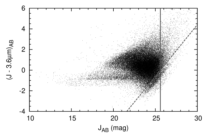
Figure 25.— $J$ and 3.6$\mu$m color-magnitude diagram. The gray solid-line indicates the 5$\sigma$ limiting magnitude for point sources in $J$, and the gray dashed-line indicates the 5$\sigma$ limit of $J$–$3.6\mu$m color for point sources. The blue galaxies with $J$ – 3.6$\mu$m $<-0.4$ start disappearing at $J>25$ (the bottom-right corner), which implies that many objects in the TENIS catalog with S/N $<$ 3 at 3.6$\mu$m are real J-detected objects.

We do not attempt to quantify the completeness of our catalog, which is nontrivial given the complex nature of IRACLEAN and the fact that we detect sources from a $J$+$K_{S}$ image. Readers interested in using our catalog and wishing to know the completeness at a given flux level should run their own source extraction and selection, quantify the completeness, and then extract photometry from our multiwavelength catalog.

9. Summary

We present an ultra-deep $J$ and $K_{S}$ dataset covering a $30\arcmin\times 30\arcmin$ area in the ECDFS, as part of our Taiwan ECDFS Near-Infrared Survey (TENIS). The median $5\sigma$ limiting magnitudes for all objects reach 24.5 and 23.9 mag (AB) for $J$ and $K_{S}$, respectively. In the inner 400 arcmin² region of the images where the sensitivity is more uniform, objects as faint as 25.6 and 25.0 mag are detected at 5 $\sigma$. In our final catalog, we detect objects in a $J$+$K_{S}$ image in order to achieve higher completeness. We also developed a novel deconvolution technique (IRACLEAN) to accurately estimate the IRAC fluxes for all the $J$+$K_{S}$ detected objects in the ECDFS, using our $J$+$K$ image as a prior. With simple Monte-Carlo simulations and comparison against the XCONV technique, we showed that IRACLEAN is able to correctly recover IRAC fluxes for most objects. We also compared IRACLEAN fluxes with fluxes directly measured by SExtractor, and with the FIRWORKS and SIMPLE catalogs. We found that IRACLEAN results are superior in many cases, and our IRACLEAN results provide by far the deepest IRAC catalog in the ECDFS region. This $J$+$K_{S}$ detected catalog consists of flux measurements for $J$, $K_{S}$, IRAC 3.6, 4.5, 5.8, and 8.0 $\mu$m, and XCONV $K_{S}$–IRAC colors for all four IRAC bands. We publicly release the data products of this work, including the $J$ and $K_{S}$ images, and the $J$+$K_{S}$ selected multiwavelength catalog.

References

- Anderson & King (2003) Anderson, J., & King, I. R. 2003, PASP, 115, 113
- Bertin & Arnouts (1996) Bertin, E. & Arnouts, S. 1996, A&AS, 117, 393
- Caldwell et al. (2008) Caldwell, J. A. R., et al. 2008, ApJS, 174, 136
- Capak et al. (2007) Capak, P., et al. 2007, ApJS, 172, 99
- Cardamone et al. (2010) Cardamone, C. N., can Dokkum, P. G., Urry, C. M., et al. 2010, ApJS, 189, 270
- Cohen et al. (2003) Cohen, M., Wheaton, Wm. A., & Megeath, S. T. 2003, AJ, 126, 1090
- Dahlen et al. (2010) Dahlen, T., et al. 2010, ApJ, 724, 425
- Damen et al. (2011) Damen, M., et al. 2011, ApJ, 727, 1
- Elston, Rieke, & Rieke (1988) Elston, R., Rieke, G. H., & Rieke, M. J. 1988, ApJ, 331, L7
- Ford et al. (2003) Ford, H. C., et al. 2003, Proc. SPIE, 4854, 81
- Franx et al. (2003) Franx, M., Labbé, I., Rudnick, G., et al. 2003, ApJ, 587, L79
- Gawiser et al. (2006) Gawiser, E., et al. 2006, ApJ, 642, L13
- Giavalisco et al. (2004) Giavalisco, M., Ferguson, H. C., Koekemoer, A. M., et al. 2004, ApJ, 600, L93
- Grazian et al. (2006) Grazian, A., et al. 2006, A&A, 449, 951
- Grogin et al. (2011) Grogin, N. A., et al. 2011, ApJS, 197, 35
- Guo et al. (2012) Guo, Y., et al. 2012, ApJ, 749, 149
- Högbom et al. (1974) Högbom, J. A. 1974, A&A Suppl., 15, 417
- Hsieh et al. (2012) Hsieh, B.C., Wang, W.-H., Yan, H., Lin, L., Karoji, H., Lim, J., Ho, P. T. P., & Tsai, C. W. 2012, ApJ, 749, 88
- Koekemoer et al. (2011) Koekemoer, A. M., et al. 2011, ApJS, 197, 36
- Kurucz (1993) Kurucz, R. L. 1993, Kurucz CD-ROM 19, ATLAS9 Stellar Atmosphere Programs and 2 kms Grid (Cambridge: SAO)
- Laidler et al. (2007) Laidler, V. G., et al. 2007, PASP, 119, 1325
- McLure et al. (2011) McLure, R. J., et al. 2011, arXiv1102.4881
- Ouchi et al. (2009) Ouchi, M., et al. 2009, ApJ, 706, 1136
- Puget et al. (2004) Puget, P., et al. 2004, SPIE, 5492, 978
- Retzlaff et al. (2010) Retzlaff, J., Rosati, P., Dickinson, M., Vandame, B., Rité, C., Nonino, M., Cesarsky, C., and the GOODS Team 2010, A&A, 511, 50
- Rix et al. (2004) Rix, H. -W., et al. 2004, ApJS, 152, 163
- Skrutskie et al. (2006) Skrutskie, M. F., et al. 2006, AJ, 131, 1163
- Sawicki (2002) Sawicki, M. 2002, AJ, 124, 3050
- Simpson & Eisenhardt (1999) Simpson, C., & Eisenhardt, P. 1999, PASP, 111, 691
- Taylor et al. (2009) Taylor, E. N. 2009, ApJS, 183, 295
- Wang et al. (2010) Wang, Wei-Hao, Cowie, Lennox L., Barger, Amy J., Keenan, Ryan C., Ting, Hsiao-Chiang 2010, ApJS, 187, 251
- Wang, Cowie, & Barger (2012) Wang, Wei-Hao, Cowie, Lennox L., & Barger, Amy J. 2012, ApJ, 744, 155
- Wolf et al. (2001) Wolf, C., Dye, S., Kleinheinrich, M., Meisenheimer, K., Rix, H.-W., Wisotzki, L. 2001, A&A, 377, 442
- Wuyts et al. (2008) Wuyts, S., Labbé, I., Förster-Schreiber, N. M., Franx, M., Rudnick, G., Brammer, G. B., & van Dokkum, P. G. 2008, ApJ, 682, 985
- Yan et al. (2004) Yan, H., Dickson, M., Eisenhardt, P. R. M., et al. 2004, ApJ, 616, 63
- Yan et al. (2011) Yan, H., et al. 2011, ApJ, 728, 22