From Quantum $A_{N}$ (Sutherland) to $E_{8}$ Trigonometric Model: Space-of-Orbits View

From Quantum $\boldsymbol{A_{N}}$ (Sutherland)
to $\boldsymbol{E_{8}}$ Trigonometric Model: Space-of-Orbits View

Alexander V. TURBINER

A.V. Turbiner

Instituto de Ciencias Nucleares, Universidad Nacional Autónoma de México,
Apartado Postal 70-543, 04510 México, D.F., Mexico turbiner@nucleares.unam.mx

Received September 21, 2012, in final form January 11, 2013; Published online January 17, 2013

A number of affine-Weyl-invariant integrable and exactly-solvable quantum models with trigonometric potentials is considered in the space of invariants (the space of orbits). These models are completely-integrable and admit extra particular integrals. All of them are characterized by (i) a number of polynomial eigenfunctions and quadratic in quantum numbers eigenvalues for exactly-solvable cases, (ii) a factorization property for eigenfunctions, (iii) a rational form of the potential and the polynomial entries of the metric in the Laplace–Beltrami operator in terms of affine-Weyl (exponential) invariants (the same holds for rational models when polynomial invariants are used instead of exponential ones), they admit (iv) an algebraic form of the gauge-rotated Hamiltonian in the exponential invariants (in the space of orbits) and (v) a hidden algebraic structure. A hidden algebraic structure for $(A{-}B{-}C{-}D)$-models, both rational and trigonometric, is related to the universal enveloping algebra $U_{gl_{n}}$. For the exceptional $(G{-}F{-}E)$-models, new, infinite-dimensional, finitely-generated algebras of differential operators occur. Special attention is given to the one-dimensional model with $BC_{1}\equiv(\mathbb{Z}_{2})\oplus T$ symmetry. In particular, the $BC_{1}$ origin of the so-called TTW model is revealed. This has led to a new quasi-exactly solvable model on the plane with the hidden algebra $sl(2)\oplus sl(2)$.

(quasi)-exact-solvability; space of orbits; trigonometric models; algebraic forms; Coxeter (Weyl) invariants; hidden algebra

35P99; 47A15; 47A67; 47A75

1 Introduction

In this article we attempt to overview our constructive knowledge of (quasi)-exactly-solvable potentials having the form of a meromorphic function in trigonometric variables. Any model with such a potential is characterized by a discrete symmetry group, and possesses an (in)finite set of polynomial eigenfunctions in a certain trigonometric variables. In the case of exactly-solvable potentials an infinite discrete spectra is quadratic in the quantum numbers. All of these models are characterized by the appearance of a hidden (Lie) algebraic structure. They do not admit a separation of variables, they are completely-integrable and possess a commutative algebra of integrals. So far, no super-integrable models with trigonometric potentials are known, although all of them admit at least one particular integral [22].

A similar overview of the rational models (with a potential in the form of a meromorphic function in Cartesian coordinates) was given in [21]. Unlike the trigonometric models the rational models do admit a separation out of radial coordinate and hence, the emergence of integral of the second order leading to super-integrability. For exactly-solvable rational models their eigenvalues depend on quantum numbers linearly, thus, their spectrum is a linear superposition of equidistant spectra.

Any spinless quantum system is characterized by the Hamiltonian

$${\cal H}=-\Delta+V(x),\qquad x\in{\mathbb{R}}^{d}.$$ (1.1)

The main problem of quantum mechanics is to find the spectrum the Hamiltonian looking for the Schrödinger equation

$${\cal H}\Psi(x)=E\Psi(x),\qquad\Psi(x)\in L^{2}\big{(}{\mathbb{R}}^{d}\big{)}.$$

in the Hilbert space. Since the Hamiltonian is a differential operator it can be represented as infinite-dimensional matrix. Thus, the solving the Schrödinger equation is equivalent to diagonalizing the infinite-dimensional matrix. It is a transcendental problem: the characteristic polynomial is of infinite order and it has infinitely-many roots. In general, we do not know how to make such a diagonalization explicitly. One can try to describe or construct quantum system for which a transcendental nature of (1.1) degenerates (completely or partially) to algebraic one: the roots of the characteristic polynomial (energies), some or all, can be found explicitly (algebraically). Usually, in such a situation one can indicate an analytic form of (some or all) eigenfunctions. Such systems do exist and we call them solvable. If all energies are known they are called exactly-solvable (ES), if only some number of them is known we call them quasi-exactly-solvable (QES) [23]. Surprisingly, almost all such models the present author is familiar with, are provided by integrable systems emerging from the Hamiltonian reduction method [13] with real, continuous coupling constants. Sometimes, these models are called the Calogero–Moser–Sutherland models. Every Hamiltonian has a discrete symmetry – it is symmetric with respect to affine Weyl group. Usually, the multi-dimensional Hamiltonians of the trigonometric models are of the form

$${\cal H}\ =\ \frac{1}{2}\sum_{k=1}^{N}\left[-\frac{\partial^{2}}{\partial y_{k}^{2}}\right]\ +\frac{\beta^{2}}{8}\sum_{\alpha\in R_{+}}\nu_{|\alpha|}(\nu_{|\alpha|}-1)\frac{|\alpha|^{2}}{\sin^{2}\frac{\beta}{2}(\alpha\cdot y)},$$ (1.2)

in the exactly-solvable case, where $R_{+}$ is a set of positive roots in the root space $\Delta$ of dimension $N$, $\beta$ is a parameter and $\mu_{|\alpha|}$ are coupling constants which depend on the root length. For roots of the same length the constants $\nu_{|\alpha|}$ are equal. Thus, the potential in (1.2) is a superposition of the Weyl-invariant functions, each defined as a sum over roots of the same length. The configuration space is the Weyl alcove. The ground state wave function has a form

$$\Psi_{0}(y)=\prod_{\alpha\in R_{+}}\left|\sin\frac{\beta}{2}(\alpha\cdot y)\right|^{\nu_{|\alpha|}}.$$ (1.3)

The ground state energy has a form $E_{0}=\beta^{2}{\epsilon}_{0}(\nu)$ and is known explicitly.

Let us take the Hamiltonian in ${\mathbb{R}}^{d}$ which is symmetric with respect to the (maximal) discrete group $G$. One can construct invariants of $G$ using a procedure of averaging some function over orbit(s). The $d$ linearly independent invariants span a linear space called the space of orbits. These invariants are generating elements of the algebra of invariants. The main idea of this paper is to study the Hamiltonian in a space of orbits (space of invariants). Technically, it implies a change of variables from the original coordinates to the invariants. Conceptually, it means factoring out the discrete symmetry of the problem. It reveals a “primary” operator of the system which being dressed by the discrete symmetry becomes the Hamiltonian.

We consider some models from the list of ones known so far.

2 Solvable models

2.1 Generalities

Many years ago, as the state-of-the-art, Sutherland found a many-body exactly-solvable and integrable Hamiltonian with trigonometric potential [18]. A few years later the Hamiltonian reduction method was introduced (for review and references see e.g. Olshanetsky–Perelomov [13]). In this method an extended family of integrable and exactly-solvable Hamiltonians with trigonometric potentials, associated with affine Weyl (Coxeter) symmetry, was found. The Sutherland model appeared as one of its representatives, the $A_{N}$ trigonometric model.

The idea of the Hamiltonian reduction method is beautiful:

• Take a simple group $G$.

• Define the Laplace–Beltrami (invariant) operator on its symmetric space (free motion).

• Radial part of the Laplace–Beltrami operator is the Olshanetsky–Perelomov Hamiltonian relevant from physical point of view. The emerging Hamiltonian is affine Weyl-symmetric, it can be associated with root system, it is integrable with integrals given by the invariant operators of order higher than two with a property of solvability.

Trigonometric case. This case appears when the coordinates of the symmetric space are introduced in such a way that a negative-curvature surface occurs. Emerging the Calogero–Moser–Sutherland–Olshanetsky–Perelomov Hamiltonian in the Cartesian coordinates has the form (1.2) with the ground state given by (1.3). In the Hamiltonian reduction, the parameters $\nu_{|\alpha|}$ of the Hamiltonian take a set of discrete values, however, they can also be generalized to any real value without loosing the property of integrability as well as solvability with the only constraint being the existence of $L^{2}$-solutions of the corresponding Schrödinger equation. The configuration space for (1.2) is the Weyl alcove.

The Hamiltonian (1.2) is completely-integrable: there exists a commutative algebra of integrals (including the Hamiltonian) of dimension which is equal to the dimension of the configuration space (for integrals, see Oshima [14] with explicit forms of those). The Hamiltonian (1.2) is invariant with respect to the affine Weyl (Coxeter) group transformation, which is the discrete symmetry group of the corresponding root space, see e.g. [13].

The Hamiltonian (1.2) has a hidden (Lie)-algebraic structure. In order to reveal it (see [1, 2, 3, 4, 12, 15, 16]) we need to

• Gauge away the ground state eigenfunction making a similarity transformation $(\Psi_{0})^{-1}({\cal H}-E_{0})\Psi_{0}=h$, then

• If the state-of-art variables are introduced for trigonometric models $A_{N}$, $BC_{N}$, $G_{2}$ and $F_{4}$ (see [1, 4, 15, 16], respectively), the Hamiltonian $h$ becomes algebraic, however,

• It can be checked, which, in fact, looks evident, that parameterizing the space of orbits of the Weyl (Coxeter) group by taking the Weyl $($Coxeter$)$ fundamental trigonometric invariants,

  $$\tau_{a}^{(\Omega)}(y;\beta)=\sum_{w\in\Omega_{a}}e^{i\beta(w,y)},$$ (2.1)

  where $\Omega_{a}$ is an orbit generated by fundamental weight $w_{a}$, $a=1,2,\ldots,N$ ($N$ is the rank of the root system); $\vec{y}$ is $N$-dimensional auxiliary vector which defines the Cartesian coordinates, as coordinates we arrive at the conclusion that the state-of-the-art variables [1, 4, 15, 16] coincide with (2.1). It should be emphasized that this fact was not clear to the authors of articles [1, 4, 15, 16] including the present author.

  From physical point of view, the expression (2.1) is a Weyl-invariant non-linear superposition of plane waves with momenta proportional to $\beta$.

The fundamental trigonometric invariants $\tau(\beta)$ taken as coordinates always lead to the gauge-rotated trigonometric Hamiltonian $h$ in a form of algebraic differential operator with polynomial coefficients. It is proved by demonstration. It is worth emphasizing a surprising fact that the period(s) of the invariants $\tau(\beta)$ is half of the period(s) of the Hamiltonian (1.2) and the ground state function (1.3). It seems correct (this can be proved by demonstration) that the original Hamiltonian ${\cal H}$ (1.2) written in terms of the fundamental trigonometric invariants $\tau(\beta)$ takes the form

$${\cal H}(\tau)=-\Delta_{g}+V(\tau),$$ (2.2)

where

$$\Delta_{g}=\frac{1}{\sqrt{g}}\partial_{\tau_{i}}\sqrt{g}g^{ij}(\tau)\partial_{\tau_{j}},$$

is the Laplace–Beltrami operator with a metric $g^{ij}(\tau)$ with polynomial in $\tau$ matrix elements, hence with polynomial in $\tau$ coefficient functions in front of the second derivatives, and with the property that the coefficient functions in front of the first derivatives are also polynomials in $\tau$; $V(\tau)$ is a rational function, see below e.g. (2.7), (2.21). The form (2.2) can be called the rational form of the trigonometric model. It is evident that the similar rational form (2.2) appears for rational models when polynomial Weyl invariants are used as new coordinates to parameterize the space of orbits. In turn, the gauge-rotated Hamiltonian $h$ in $\tau$-variables takes the form

$$h(\tau)=-\Delta_{g}+\sum_{\alpha\in R_{+}}\nu_{|\alpha|}\sum_{a=1,\ldots,N}C_{a}^{|\alpha|}(\tau)\partial_{\tau_{a}},$$

where $C_{a}(\tau)$ are polynomials in $\tau$, see below e.g. (2.9), (2.27). The same representation is valid for the rational models.

2.2 $\boldsymbol{A_{1}/BC_{1}}$ case or trigonometric Pöschl–Teller potential

The $BC_{1}$ trigonometric Hamiltonian reads

$${\cal H}_{BC_{1}}(x)=-\frac{d^{2}}{d{x}^{2}}+\frac{g_{2}\beta^{2}}{\sin^{2}\beta x}+\frac{g_{3}\beta^{2}}{4\sin^{2}{\frac{\beta x}{2}}},$$ (2.3)

where $\beta$, $g_{2}$, $g_{3}$ are parameters. Symmetry: $(\mathbb{Z}_{2})\oplus T$ (reflections $x\rightarrow-x$, translation $x\rightarrow x+2\pi/\beta$). As for the configuration space, it can be taken the interval $[0,\frac{\pi}{\beta}]$. If $g_{2}=0$ the interval can be extended to $[0,\frac{2\pi}{\beta}]$. At $g_{3}=0$ (or $g_{2}=0$) the Hamiltonian (2.3) degenerates to the $A_{1}$ trigonometric Hamiltonian, which describes the relative motion of two particle system on a line.

The ground state for (2.3) reads

$$\Psi_{0}=\big{|}\sin(\beta x)\big{|}^{\nu_{2}}\left|\sin\left({\frac{\beta}{2}{x}}\right)\right|^{\nu_{3}},\qquad E_{0}=-\left(\nu_{2}+\frac{\nu_{3}}{2}\right)^{2}\beta^{2},$$ (2.4)

cf. (1.3), where $\nu_{2}$, $\nu_{3}$ are found from the relations

$$g_{2}=\nu_{2}(\nu_{2}-1)>-\frac{1}{4},\qquad g_{3}=\nu_{3}(\nu_{3}+2\nu_{2}-1)>-\frac{1}{4}.$$

Note that if the parameters in (2.3) are related $g_{2}=\frac{g_{3}}{2}(\frac{g_{3}}{2}-1)$, the ground state energy (2.4) reaches its maximal value, $E_{0}=0$.

Any eigenfunction has a form $\Psi_{0}\varphi$, where $\varphi$ is a polynomial in the $BC_{1}$ fundamental trigonometric invariant $\tau(\beta)=\cos(\beta x)$ (see (2.1)). Hence, the ground state function $\Psi_{0}$ plays a role of a multiplicative factor.

The $BC_{1}$ trigonometric Hamiltonian (2.3) is easily related to the trigonometric Pöschl–Teller (PT) Hamiltonian

$${\cal H}_{\rm PT}=-\frac{d^{2}}{d{x}^{2}}+\frac{\big{(}\alpha^{2}-\frac{1}{4}\big{)}\beta^{2}}{4\sin^{2}\frac{\beta x}{2}}+\frac{\big{(}\gamma^{2}-\frac{1}{4}\big{)}\beta^{2}}{4\cos^{2}\frac{\beta x}{2}},$$ (2.5)

where

$$\alpha^{2}-\frac{1}{4}=g_{2}+g_{3},\qquad\gamma^{2}-\frac{1}{4}=g_{2}.$$

Replacing in (2.5) $\beta\rightarrow i\beta$, we arrive at the general hyperbolic Pöschl–Teller Hamiltonian

$${\cal H}_{\rm PT}^{(h)}=-\frac{d^{2}}{d{x}^{2}}+\frac{\big{(}\alpha^{2}-\frac{1}{4}\big{)}\beta^{2}}{4\sinh^{2}\frac{\beta x}{2}}-\frac{\big{(}\gamma^{2}-\frac{1}{4}\big{)}\beta^{2}}{4\cosh^{2}\frac{\beta x}{2}},$$

while the one-soliton Hamiltonian appears at $\alpha^{2}=\frac{1}{4}$. In the case of the $BC_{1}$ trigonometric Hamiltonian under the replacement $\beta\rightarrow i\beta$ the $BC_{1}$ Hyperbolic Hamiltonian occurs.

Let us introduce a new variable

$$\tau=\cos(\beta x)$$ (2.6)

(which is the $\frac{2\pi}{\beta}$-periodic, $BC_{1}$-Weyl invariant) in the $BC_{1}$ Hamiltonian (2.3). It appears that

$${\cal H}_{BC_{1}}(\tau)=-\Delta_{g}+\frac{g_{2}}{2(1+\tau)}+\frac{(g_{2}+g_{3})}{2(1-\tau)},$$ (2.7)

with amazingly simple meromorphic potential, where

$$\Delta_{g}=\big{(}\tau^{2}-1\big{)}\frac{d^{2}}{d{\tau}^{2}}+\tau\frac{d}{d{\tau}}$$

is the flat Laplace–Beltrami operator with metric $g^{11}=\big{(}\tau^{2}-1\big{)}$. Overall multiplicative factor $\beta^{2}$ in (2.7) is dropped off. It can be called a rational form of the $BC_{1}$ trigonometric Hamiltonian. The eigenvalue problem for (2.7) is considered on the interval $[-1,1]$. It can be easily seen that the rational form for the $BC_{1}$ hyperbolic Hamiltonian is exactly the same as for the $BC_{1}$ trigonometric Hamiltonian (!) and is given by (2.7). However, the domain for the $BC_{1}$ hyperbolic Hamiltonian (2.7) is $[1,\infty)$. In the hyperbolic case taking $\tau=\cosh{\beta x}$ (cf. (2.6)) we obtain the same Hamiltonian (2.7). The ground state eigenfunction (2.4) in $\tau$ coordinate (2.6) becomes

$$\Psi_{0}(\tau)=(1+\tau)^{\frac{\nu_{2}}{2}}(1-\tau)^{\frac{\nu_{2}+\nu_{3}}{2}}.$$ (2.8)

At $\nu_{2}=1$ and $\nu_{3}=0$ it coincides to the Jacobian.

Now let us make a gauge rotation

$$h_{BC_{1}}=\frac{1}{\beta^{2}}\Psi_{0}^{-1}({\cal H}_{BC_{1}}-E_{0})\Psi_{0},$$

with $\Psi_{0}$ given by (2.4) and write the result in the variable $\tau$. After a simple calculations it reads

$$h_{BC_{1}}(\tau)=\big{(}\tau^{2}-1\big{)}\frac{d^{2}}{d{\tau}^{2}}+[(2\nu_{2}+\nu_{3}+1)\tau+\nu_{3}]\frac{d}{d{\tau}},$$ (2.9)

which is the algebraic form of the ${BC_{1}}$ Hamiltonian (2.3). Its eigenvalues are

$$\epsilon_{p}=p^{2}+(2\nu_{2}+\nu_{3})p,\qquad p=0,1,2,\ldots,$$ (2.10)

being quadratic in quantum number $p$, while the eigenfunctions are the Jacobi polynomials, $\varphi_{p}=P_{p}^{(\nu_{2}+\nu_{3}-\frac{1}{2},\nu_{2}-\frac{1}{2})}(\tau)$. Eventually, the explicit form of an eigenfunction of the Hamiltonian (2.3) is

$$\Psi_{p}^{(BC_{1})}=P_{p}^{(\nu_{2}+\nu_{3}-\frac{1}{2},\nu_{2}-\frac{1}{2})}(\cos(\beta x))\big{|}\sin(\beta x)\big{|}^{\nu_{2}}\left|\sin\left({\frac{\beta}{2}{x}}\right)\right|^{\nu_{3}},\qquad p=0,1,2,\ldots.$$

It can be easily checked that the gauge-rotated Hamiltonian $h_{BC_{1}}(\tau)$ has infinitely many finite-dimensional invariant subspaces

$${\cal P}_{n}=\langle\tau^{p}|0\leq p_{1}\leq n\rangle,\qquad n=0,1,2,\ldots,$$ (2.11)

hence, the infinite flag ${\cal P}$,

$${\cal P}_{0}\subset{\cal P}_{1}\subset{\cal P}_{2}\subset\cdots\subset{\cal P}_{n}\subset\cdots\subset{\cal P},$$

with the characteristic vector $\vec{f}=(1)$ (see below), is preserved by $h_{BC_{1}}$. Thus, the eigenfunctions of $h_{BC_{1}}$ are elements of the flag ${\cal P}$. Any subspace ${\cal P}_{n}$ contains $(n+1)$ eigenfunctions which is equal to $\dim{\cal P}_{n}$.

Take the algebra $gl_{2}$ in $(n+1)$-dimensional representation realized by the first order differential operators

$$J^{-}=\frac{d}{d\tau},\qquad J^{0}_{n}=\tau\frac{d}{d\tau}-n,\qquad T^{0}=1,\qquad J^{+}_{n}={\tau}^{2}\frac{d}{d\tau}-nt=\tau J^{0}_{n},$$ (2.12)

where $n=0,1,\ldots$ and $T^{0}$ is the central element. Its finite-dimensional representation space is the space of polynomials ${\cal P}_{n}$ (2.11). Hence, the finite-dimensional invariant subspaces of the Hamiltonian $h_{BC_{1}}$ coincide with the finite-dimensional representation spaces of $gl_{2}$ (2.12) for $n=0,1,2,\ldots$. It immediately implies that the algebra $gl_{2}$ is the hidden algebra of the ${BC_{1}}$ trigonometric Hamiltonian – it can be written in terms of $gl_{2}$ generators (2.12)

$$h_{BC_{1}}=J^{0}J^{0}-J^{-}J^{-}+(2\nu_{2}+\nu_{3}+1)J^{0}+\nu_{3}J^{-},$$ (2.13)

where $J^{0}\equiv J^{0}_{0}$, $J^{-}\equiv J^{-}_{0}$. Thus, the Hamiltonian $h_{BC_{1}}$ is an element of the universal enveloping algebra $U_{gl_{2}}$.

Among the generators of the algebra $gl_{2}$ (2.12) there is the Euler-Cartan operator,

$$J^{0}_{n}=\tau\frac{d}{d\tau}-n,$$

which has zero grading; it maps a monomial in $\tau$ to itself. It defines the highest weight vector. This generator allows us to construct a particular integral – $\pi$-integral of zero grading of the $(n+1)$th order (see [22]) $i_{\rm par}^{(n)}(\tau)$: its commutator with $h_{BC_{1}}$ vanishes on a subspace. If

$$i_{\rm par}^{(n)}(\tau)=\prod_{j=0}^{n}\big{(}J^{0}_{n}+j\big{)},$$ (2.14)

then

$$\big{[}h_{BC_{1}}(\tau),i_{\rm par}^{(n)}(\tau)\big{]}:\ {\cal P}_{n}\mapsto 0.$$

Making the gauge rotation of the $\pi$-integral (2.14) with $\Psi_{0}^{-1}(\tau)$ given by (2.4) and changing variables $\tau$ back to the Cartesian coordinate we arrive at the quantum $\pi$-integral acting in the Hilbert space,

$${\cal I}_{{\rm par},BC_{1}}^{(n)}(x)=\left.\Psi_{0}(\tau)i_{\rm par}^{(n)}(\tau)\Psi_{0}^{-1}(\tau)\right|_{\tau\rightarrow x}.$$

Under such a gauge transformation the triangular space of polynomials ${\cal P}_{n}$ becomes the space

$${\cal V}_{n}=\Psi_{0}{\cal P}_{n}.$$

The Hamiltonian ${\cal H}_{BC_{1}}(x)$ commutes with ${\cal I}_{{\rm par},BC_{1}}^{(n)}(x)$ over this space

$$\big{[}{\cal H}_{BC_{1}}(x),{\cal I}_{{\rm par},BC_{1}}^{(n)}(x)\big{]}:\ {\cal V}^{(N-1)}_{n}\mapsto 0.$$

Any eigenfunction $\Psi\in{\cal V}_{n}$ is zero mode of the $\pi$-integral ${\cal I}_{{\rm par},BC_{1}}^{(n)}(x)$.

It is worth noting a connection of the $BC_{1}$ trigonometric model with the so-called Tremblay–Turbiner–Winternitz (TTW) model [19] and, in particular, with the $I_{2}(k)$ rational model (see e.g. [21]). In order to see it let us combine the $BC_{1}$ trigonometric Hamiltonian ${\cal H}_{BC_{1}}(\phi)$ (2.3) as the angular part and the radial part of two-dimensional spherical-symmetrical harmonic oscillator Hamiltonian as the radial part forming the 2D Hamiltonian

$${\cal H}_{\rm TTW}(r,\phi;\omega,\nu_{2},\nu_{3},\beta)=-\partial_{r}^{2}-\frac{1}{r}\partial_{r}+\omega^{2}r^{2}+\frac{{\cal H}_{BC_{1}}(\phi)}{r^{2}},$$ (2.15)

which is nothing but the Hamiltonian of the TTW model [19]. If $\beta=k$ is integer, this Hamiltonian corresponds to the $I_{2}(k)$ rational model [13]. Since the both Hamiltonians are exactly-solvable, the TTW model is also exactly-solvable but with spectra of two-dimensional anisotropic (!) harmonic oscillator with frequency ratio $1:\beta$. Any eigenfunction of (2.15) has the form of a polynomial $p(r^{2},\cos(\beta\phi))$ in variables $r^{2}$ and $\cos(\beta\phi)$ multiplied by a ground state function

$$\Psi_{0}^{\rm(TTW)}(r,\phi)=r^{(\nu_{2}+\nu_{3})\beta}\big{|}\sin(\beta\phi)\big{|}^{\nu_{2}}\left|\sin\left({\frac{\beta}{2}{\phi}}\right)\right|^{\nu_{3}}e^{-\frac{\omega r^{2}}{2}},$$ (2.16)

namely,

$$\Psi^{\rm(TTW)}(r,\phi)=p\left(r^{2},\cos(\beta\phi)\right)\Psi_{0}^{\rm(TTW)}(r,\phi).$$

If in the construction (2.15) instead of two-dimensional radial harmonic oscillator, the radial Hamiltonian of the sextic QES $2D$ central potential (see e.g. [23]) is taken, the quasi-exactly-solvable extension of the TTW model occurs [19]

$${\cal H}_{\rm TTW}^{\rm(qes)}(r,n;\phi;\omega,\nu_{2},\nu_{3},\beta,a)=-\partial_{r}^{2}-\frac{1}{r}\partial_{r}+a^{2}r^{6}+2a\omega r^{4}$$

$$\hphantom{{\cal H}_{\rm TTW}^{\rm(qes)}(r,n;\phi;\omega,\nu_{2},\nu_{3},\beta,a)=}{}+\left[\omega^{2}-2a(2n+2+\beta(\nu_{2}+\nu_{3}))\right]r^{2}+\frac{{\cal H}_{BC_{1}}(\phi)}{r^{2}},$$ (2.17)

cf. (2.15), here $n$ is non-negative integer and $a>0$ is a parameter. In this Hamiltonian a finite number of eigenstates can be found explicitly (algebraically). Their eigenfunctions have the form of a polynomial $p(r^{2},\cos(\beta\phi))$ of degree $n$ in $r^{2}$ multiplied by a factor

$$\Psi_{0}^{\rm(qes,TTW)}=r^{(\nu_{2}+\nu_{3})\beta}\big{|}\sin(\beta\phi)\big{|}^{\nu_{2}}\left|\sin\left({\frac{\beta}{2}{\phi}}\right)\right|^{\nu_{3}}e^{-\frac{\omega r^{2}}{2}-\frac{ar^{4}}{4}},$$ (2.18)

cf. (2.16), namely,

$$\Psi_{\rm alg}^{\rm(qes,TTW)}=p\left(r^{2},\cos(\beta\phi)\right)\Psi_{0}^{\rm(qes,TTW)}.$$

The factor (2.18) is the ground state eigenfunction of the Hamiltonian (2.17) at $n=0$. If $\beta$ is equal to non-negative integer $k$, a polynomial $p(r^{2},\cos(\beta\phi))$ belongs to the space ${\cal P}_{(1,k)}$ with the characteristic vector $\vec{f}=(1,k)$, see below.

2.3 Quasi-exactly-solvable $\boldsymbol{BC_{1}}$ case
(or QES trigonometric Pöschl–Teller potential)

The Hamiltonian $h_{BC_{1}}(\tau)$ (2.9) is $gl(2)$-Lie-algebraic operator (2.13) which has infinitely-many finite-dimensional invariant subspaces in polynomials (2.11). By adding to $h_{BC_{1}}(\tau)$ (2.9) the operator

$$\delta h^{\rm(qes)}(\tau)=2b\big{(}\tau^{2}-1\big{)}\frac{d}{d\tau}-2bn\tau+2b\left(n+\nu_{2}+\nu_{3}+\frac{1}{2}\right),$$

where $b$ is a parameter and $n$ is non-negative integer, as a result we get the operator

$$h_{BC_{1}}^{\rm(qes)}(\tau)=h_{BC_{1}}+\delta h^{\rm(qes)},$$ (2.19)

which has a single finite-dimensional invariant subspace

$${\cal P}_{n}=\langle\tau^{p}\,|\,0\leq p\leq n\rangle,$$

of the dimension $(n+1)$. Hence, this operator is quasi-exactly-solvable - it can be written in terms of $gl_{2}$ generators in $(n+1)$-dimensional representation (2.12),

$$h_{BC_{1}}^{\rm(qes)}=J^{0}_{n}J^{0}_{n}-J^{-}J^{-}-2bJ^{+}_{n}+(2n+2\nu_{2}+\nu_{3}+1)J^{0}_{n}+(\nu_{3}-2b)J^{-}$$

$$\phantom{h_{BC_{1}}^{\rm(qes)}=}{}+n(n+2\nu_{2}+\nu_{3}+1).$$

Making the gauge rotation of (2.19) with

$$\tilde{\Psi}_{0}=e^{-\frac{\nu_{2}+\nu_{3}}{2}\log(1-\tau)-\frac{\nu_{2}}{2}\log(1+\tau)}e^{b\tau}$$

and the change of variable $\tau=\cos(\beta x)$ we arrive at the $BC_{1}$-trigonometric QES Hamiltonian [23]

$${\cal H}_{BC_{1}}^{\rm(qes)}(x)=-\frac{d^{2}}{d{x}^{2}}+\frac{\nu_{2}(\nu_{2}-1)\beta^{2}}{\sin^{2}\beta x}+\frac{\nu_{3}(\nu_{3}+2\nu_{2}-1)\beta^{2}}{4\sin^{2}{\frac{\beta x}{2}}}+b^{2}\beta^{2}{\sin^{2}\beta x}$$

$$\phantom{{\cal H}_{BC_{1}}^{\rm(qes)}(x)=}{}+2b\beta^{2}(2n+2\nu_{2}+\nu_{3}+1)\sin^{2}{\frac{\beta x}{2}},$$ (2.20)

cf. (2.3), where $b$, $\nu_{2}$, $\nu_{3}$, $\beta$ are parameters, $n$ is non-negative integer. In $\tau$-variable (2.6) the $BC_{1}$-trigonometric QES Hamiltonian appears in rational form

$${\cal H}_{BC_{1}}^{\rm(qes)}(\tau)=-\Delta_{g}+\frac{g_{2}}{\big{(}1\!-\!\tau^{2}\big{)}}+\frac{g_{3}}{2(1\!-\!\tau)}+b^{2}\big{(}1\!-\!\tau^{2}\big{)}+b(2n+2\nu_{2}+\nu_{3}+1)(1\!-\!\tau),$$ (2.21)

cf. (2.7), where $\Delta_{g}=(\tau^{2}-1)\frac{d^{2}}{d{\tau}^{2}}+\tau\frac{d}{d{\tau}}$ is the flat Laplace–Beltrami operator with metric $g^{11}=(\tau^{2}-1)$. Overall multiplicative factor $\beta^{2}$ in (2.20) is dropped off.

In the Hamiltonian (2.20) the $(n+1)$ eigenfunctions are of a form

$$P_{n}(\cos(\beta x))\big{|}\sin(\beta x)\big{|}^{\nu_{2}}\left|\sin\left({\frac{\beta}{2}{x}}\right)\right|^{\nu_{3}}e^{-b\cos(\beta x)},$$

where $P_{n}(\tau)$ is a polynomial of degree $n$, they can be found by algebraic means. It is evident that $i_{\rm par}^{(n)}(\tau)$ (2.14) remains the particular integral – $\pi$-integral of the $BC_{1}$-trigonometric QES Hamiltonian (2.19) (see [22])

$$\big{[}h_{BC_{1}}^{\rm(qes)}(\tau),i_{\rm par}^{(n)}(\tau)\big{]}:\ {\cal P}_{n}\mapsto 0.$$

Interestingly, the $BC_{1}$-trigonometric QES Hamiltonian (2.20) degenerates to the so-called Magnus–Winkler (MW) Hamiltonian or, in other words, to the QES Lame Hamiltonian (see e.g. [23])

$${\cal H}_{BC_{1}}^{\rm(qes)}=-\frac{d^{2}}{d{x}^{2}}+b^{2}\beta^{2}{\sin^{2}\beta x}+2b\beta^{2}(2n+\nu+1)\sin^{2}{\frac{\beta x}{2}},$$

where $\nu=0,1$.

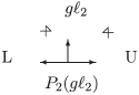
For $\nu=0$ and given $n$ there exist two families of eigenfunctions

$$\varphi^{(0,+)}_{n,i}=P_{n}(\cos(\beta x))e^{-b\cos(\beta x)},\qquad i=0,1,\ldots,n,$$

$$\varphi^{(0,-)}_{n-1,i}=P_{n-1}(\cos(\beta x))\sin(\beta x)e^{-b\cos(\beta x)},\qquad i=0,1,\ldots,n-1,$$

which correspond to periodic (anti-periodic) boundary conditions, correspondingly. These eigenfunctions describe lower (upper) edges of Brillouin zones, respectively. Polynomial factors in $\varphi^{(0,+)}_{n,i}$ and $\varphi^{(0,-)}_{n-1,i}$ are eigenfunctions of

$$h_{BC_{1}}^{({\rm qes},0,+)}=J^{0}_{n}J^{0}_{n}-J^{-}J^{-}-2bJ^{+}_{n}+(2n+1)J^{0}_{n}-2bJ^{-}+n(n+1),$$

$$h_{BC_{1}}^{({\rm qes},0,-)}=J^{0}_{n-1}J^{0}_{n-1}-J^{-}J^{-}-2bJ^{+}_{n-1}+(2n+1)J^{0}_{n-1}-2bJ^{-}+n(n+2),$$

respectively (see (2.12)).

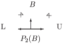
For $\nu=1$ and given $n$ there also exist two families of eigenfunctions

$$\varphi^{(1,-)}_{n,i}=P_{n}(\cos(\beta x))\sin\left({\frac{\beta}{2}{x}}\right)e^{-b\cos(\beta x)},\qquad i=0,1,\ldots,n,$$

$$\varphi^{(1,+)}_{n,i}=P_{n}(\cos(\beta x))\cos\left({\frac{\beta}{2}{x}}\right)e^{-b\cos(\beta x)},\qquad i=0,1,\ldots,n,$$

which correspond to (anti)-periodic boundary conditions, correspondingly. These eigenfunctions describe upper (lower) edges of Brillouin zones, respectively. Polynomial factors in $\varphi^{(1,-)}_{n,i}$ and $\varphi^{(1,+)}_{n,i}$ are eigenfunctions of

$$h_{BC_{1}}^{({\rm qes},1,-)}=J^{0}_{n}J^{0}_{n}-J^{-}J^{-}-2bJ^{+}_{n}+2(n+1)J^{0}_{n}+(1-2b)J^{-}+n(n+2),$$

$$h_{BC_{1}}^{({\rm qes},1,+)}=J^{0}_{n}J^{0}_{n}-J^{-}J^{-}-2bJ^{+}_{n}+2(n+1)J^{0}_{n}-(1+2b)J^{-}+n(n+2),$$

respectively (see (2.12)).

If in a construction (2.15) to obtain the TTW model we replace the $BC_{1}$-trigonometric Hamiltonian ${\cal H}_{BC_{1}}(\phi)$ (2.3) by the $BC_{1}$-trigonometric QES Hamiltonian ${\cal H}_{BC_{1}}^{\rm(qes)}(\phi)$ (2.19)

$${\cal H}_{\rm TTW}^{\rm(qes)}(r,\phi;\omega,\nu_{2},\nu_{3},\beta)=-\partial_{r}^{2}-\frac{1}{r}\partial_{r}+\omega^{2}r^{2}+\frac{{\cal H}_{BC_{1}}^{\rm(qes)}(\phi)}{r^{2}},$$

a new quasi-exactly-solvable extension of the TTW model is obtained

$$\tilde{\cal H}_{\rm TTW}^{\rm(qes)}(r;\phi,m;\omega,\nu_{2},\nu_{3},\beta,b)=-\Delta^{(2)}+\omega^{2}r^{2}+\frac{\nu_{2}(\nu_{2}-1)\beta^{2}}{r^{2}\sin^{2}\beta\phi}+\frac{\nu_{3}(\nu_{3}+2\nu_{2}-1)\beta^{2}}{4r^{2}\sin^{2}{\frac{\beta\phi}{2}}}$$

$$\qquad{}+\frac{b^{2}\beta^{2}{\sin^{2}\beta\phi}}{r^{2}}+\frac{2b\beta^{2}(2m+2\nu_{2}+\nu_{3}+1)\sin^{2}{\frac{\beta\phi}{2}}}{r^{2}},$$

cf. (2.15), where $\Delta^{(2)}$ is $2D$ Laplacian, $b$, $\nu_{2}$, $\nu_{3}$, $\beta$ are parameters, $m$ is non-negative integer.

If in the construction (2.15) instead of two-dimensional radial harmonic oscillator, the radial Hamiltonian of the sextic QES $2D$ radial potential [23] is taken and the $BC_{1}$-trigonometric Hamiltonian ${\cal H}_{BC_{1}}(\phi)$ (2.3) is replaced by the $BC_{1}$-trigonometric QES Hamiltonian ${\cal H}_{BC_{1}}^{\rm(qes)}(\phi)$ (2.19) the most general quasi-exactly-solvable extension of the TTW model occurs

$$\hat{\cal H}_{\rm TTW}^{\rm(qes)}(r,n;\phi,m;\omega,\nu_{2},\nu_{3},\beta,a,b)=-\Delta^{(2)}+a^{2}r^{6}+2a\omega r^{4}$$

$$\qquad{}+\left[\omega^{2}-2a(2n+2+\beta(\nu_{2}+\nu_{3}))\right]r^{2}+\frac{\nu_{2}(\nu_{2}-1)\beta^{2}}{r^{2}\sin^{2}\beta\phi}+\frac{\nu_{3}(\nu_{3}+2\nu_{2}-1)\beta^{2}}{4r^{2}\sin^{2}{\frac{\beta\phi}{2}}}$$

$$\qquad{}+\frac{b^{2}\beta^{2}{\sin^{2}\beta\phi}}{r^{2}}+\frac{2b\beta^{2}(2m+2\nu_{2}+\nu_{3}+1)\sin^{2}{\frac{\beta\phi}{2}}}{r^{2}},$$ (2.22)

where $n$, $m$ is non-negative integer and $a>0$, $b$ are parameters. In this Hamiltonian a finite number of eigenstates can be found explicitly (algebraically). Their eigenfunctions have the form of a polynomial $p\left(r^{2},\cos(\beta\phi)\right)$ of degree $n$ in $r^{2}$ and of degree $m$ in $\cos(\beta x)$ multiplied by a factor

$$\hat{\Psi}_{0}^{\rm(qes,TTW)}(r,\phi)=r^{(\nu_{2}+\nu_{3})\beta}\big{|}\sin(\beta\phi)\big{|}^{\nu_{2}}\left|\sin\left({\frac{\beta}{2}{\phi}}\right)\right|^{\nu_{3}}e^{-\frac{\omega r^{2}}{2}-\frac{ar^{4}}{4}-b\cos(\beta\phi)},$$ (2.23)

cf. (2.16), namely,

$$\hat{\Psi}_{\rm alg}^{\rm(qes,TTW)}(r,\phi)=p\left(r^{2},\cos(\beta\phi)\right)\hat{\Psi}_{0}^{\rm(qes,TTW)}(r,\phi).$$

The factor (2.23) becomes the ground state eigenfunction of the Hamiltonian (2.22) at $n\!=\!m\!=\!0$.

2.4 Case $\boldsymbol{A_{N-1}}$

Figure 1: $N$-body Sutherland model.

This is the celebrated Sutherland model ($A_{N-1}$ trigonometric model) which was found in [18]. It describes $N$ identical particles on a circle (see Fig. 1) with singular pairwise interaction $\propto\frac{1}{h^{2}}$ where $h$ is the horde. The Hamiltonian is

$${\cal H}_{\rm Suth}=-\frac{1}{2}\sum_{k=1}^{N}\frac{\partial^{2}}{\partial x_{k}^{2}}+\frac{g\beta^{2}}{4}\sum_{k<l}^{N}\frac{1}{\sin^{2}\big{(}\frac{\beta}{2}(x_{k}-x_{l})\big{)}},$$ (2.24)

where $g$ is the coupling constant and $\beta$ is a parameter. The symmetry of the system is $S_{N}\oplus T\oplus\mathbb{Z}_{2}$ (permutations $x_{i}\rightarrow x_{j}$, translation $x_{i}\rightarrow x_{i}+2\pi/\beta$ and all $x_{i}\rightarrow-x_{i}$). The ground state of the Hamiltonian (2.24) reads

$$\Psi_{0}(x)=\prod_{i<j}\left|\sin^{2}\left(\frac{\beta}{2}(x_{i}-x_{j})\right)\right|^{\nu},\qquad g=\nu(\nu-1)\geq-\frac{1}{4}$$ (2.25)

(cf. (1.3)). Let us make the gauge rotation

$$h_{\rm Suth}=\frac{2}{\beta^{2}}\Psi_{0}^{-1}({\cal H}_{\rm Suth}-E_{0})\Psi_{0},$$

where $E_{0}$ is the ground state energy. Then introduce center-of-mass variables

$$Y=\sum x_{i},\qquad y_{i}=x_{i}-\frac{1}{N}Y,\qquad i=1,\ldots,N,$$

here $\sum\limits^{N}_{i=1}y_{i}=0$, and then new permutationally-symmetric, translationally-invariant, periodic relative variables [16]

$$(x_{1},x_{2},\ldots x_{N})\rightarrow\big{(}Y,\ \tau_{n}(x)=\sigma_{n}\big{(}e^{i\beta y(x)}\big{)}\,\big{|}\,{n=1,2,3,\ldots,(N-1)}\big{)},$$ (2.26)

where

$$\sigma_{k}(x)=\sum_{i_{1}<i_{2}<\cdots<i_{k}}x_{i_{1}}x_{i_{2}}\cdots x_{i_{k}},\qquad\sigma_{k}(-x)=(-)^{k}\sigma_{k}(x),$$

are elementary symmetric polynomials, and

$$\tau_{0}=\tau_{N}(x)=1,\qquad\tau_{k}(x)=0,\qquad k<0\quad\text{or}\quad k>N.$$

The ground state function (2.25) in $\tau$-variables takes a form of a polynomial in some power, e.g.

$$\Psi_{0}^{(A_{2})}(x)=\left(4\tau_{1}^{3}+4\tau_{2}^{3}-18\tau_{1}\tau_{2}-\tau_{1}^{2}\tau_{2}^{2}+27\right)^{\frac{\nu}{2}}.$$

After the center-of-mass separation, the gauge rotated Hamiltonian takes the algebraic form [16]

$$h_{\rm Suth}=\sum_{i,j=1}^{N-1}{\cal A}_{ij}(\tau)\frac{\partial^{2}}{\partial{\tau_{i}}\partial{\tau_{j}}}+\sum_{i=1}^{N-1}{\cal B}_{i}(\tau)\frac{\partial}{\partial\tau_{i}},$$ (2.27)

where

$${\cal A}_{ij}=\frac{(N-i)j}{N}\tau_{i}\tau_{j}+\sum_{{l\geq}{\max(1,j-i)}}(j-i-2l)\tau_{i+l}\tau_{j-l},\qquad{\cal B}_{i}=\left(\frac{1}{N}+\nu\right)i(N-i)\tau_{i},$$

Eigenvalues of the gauge-rotated Hamiltonian (2.27) are

$$N\epsilon_{\{p\}}=\nu N\sum_{i=1}^{N-1}i(N-i)p_{i}+\sum_{i,j=1}^{N-1}{(N-i)j}p_{i}p_{j},$$

being quadratic in quantum numbers $\{p_{1},p_{2},\ldots,p_{(N-1)}\}$ where $p_{1},p_{2},\ldots,p_{(N-1)}=0,1,2,\ldots$.

It is easy to check that the gauge-rotated Hamiltonian $h_{\rm Suth}$ has infinitely many finite-dimensional invariant subspaces

$${\cal P}_{n}^{(N-1)}=\big{\langle}{\tau_{1}}^{p_{1}}{\tau_{2}}^{p_{2}}\cdots{\tau_{(N-1)}}^{p_{N-1}}\,|\,0\leq\sum p_{i}\leq n\big{\rangle}.$$ (2.28)

where $n=0,1,2,\ldots$. As a function of $n$ the spaces ${\cal P}_{n}^{(N-1)}$ form the infinite flag (see below).

2.4.1 The $\boldsymbol{gl_{d+1}}$-algebra acting by 1st order differential operators in $\boldsymbol{{\mathbb{R}}^{d}}$

It can be checked by the direct calculation that the $gl_{d+1}$ algebra realized by the first-order differential operators acting in ${\mathbb{R}}^{d}$ in the representation given by the Young tableaux as a row $(n,\underbrace{0,0,\ldots,0}_{d-1})$ has a form

$${\cal J}_{i}^{-}=\frac{\partial}{\partial\tau_{i}},\quad i=1,2,\ldots,d,\qquad{{\cal J}_{ij}}^{0}=\tau_{i}\frac{\partial}{\partial\tau_{j}},\quad i,j=1,2,\ldots,d,$$

$${\cal J}^{0}=\sum_{i=1}^{d}\tau_{i}\frac{\partial}{\partial\tau_{i}}-n,\qquad{\cal J}_{i}^{+}=\tau_{i}{\cal J}^{0}=\tau_{i}\left(\sum_{j=1}^{d}\tau_{j}\frac{\partial}{\partial\tau_{j}}-n\right),\quad i=1,2,\ldots,d,$$ (2.29)

where $n$ is an arbitrary number. The total number of generators is $(d+1)^{2}$. If $n$ takes the integer values, $n=0,1,2,\ldots$, the finite-dimensional irreps occur

$${\cal P}_{n}^{(d)}=\big{\langle}{\tau_{1}}^{p_{1}}{\tau_{2}}^{p_{2}}\cdots{\tau_{d}}^{p_{d}}\,|\,0\leq\sum p_{i}\leq n\big{\rangle}$$

(cf. (2.28)). It is a common invariant subspace for (2.29). The spaces ${\cal P}_{n}^{(d)}$ at $n=0,1,2,\ldots$ can be ordered

$${\cal P}_{0}^{(d)}\subset{\cal P}_{1}^{(d)}\subset{\cal P}_{2}^{(d)}\subset\cdots\subset{\cal P}_{n}^{(d)}\subset\cdots\subset{\cal P}^{(d)}.$$ (2.30)

Such a nested construction is called infinite flag $($filtration$)$ ${\cal P}^{(d)}$. It is worth noting that the flag ${\cal P}^{(d)}$ is made out of finite-dimensional irreducible representation spaces ${\cal P}_{n}^{(d)}$ of the algebra $gl_{d+1}$ taken in realization (2.29). It is evident that any operator made out of generators (2.29) has finite-dimensional invariant subspace which is finite-dimensional irreducible representation space.

2.4.2 Algebraic properties of the Sutherland model

It seems evident that the Hamiltonian (2.27) has to have a representation as a second order polynomial in generators (2.29) at $d=N-1$ acting in ${\mathbb{R}}^{N-1}$,

$$h_{\rm Suth}=\operatorname{Pol}_{2}\big{(}{\cal J}_{i}^{-},{{\cal J}_{ij}}^{0}\big{)},$$

where the raising generators ${\cal J}_{i}^{+}$ are absent. Thus, $gl(N)$ (or, strictly speaking, its maximal affine subalgebra) is the hidden algebra of the $N$-body Sutherland model. Hence, $h_{\rm Suth}$ is an element of the universal enveloping algebra ${\cal U}_{gl(N)}$. The eigenfunctions of the $N$-body Sutherland model are elements of the flag of polynomials ${\cal P}^{(N-1)}$. Each subspace ${\cal P}_{n}^{(N-1)}$ is represented by the Newton polytope (pyramid). It contains $C^{N-1}_{n+N-1}$ eigenfunctions, which is equal to the volume of the Newton polytope. They are orthogonal with respect to $\Psi_{0}^{2}$, see (2.25).

The Hamiltonian (2.24) is completely-integrable: there exists a commutative algebra of integrals (including the Hamiltonian and the momentum of the center-of-mass motion) of dimension $N$ which is equal to the dimension of the configuration space (for integrals, see Oshima [14] with explicit forms of those). Each integral ${\cal I}_{k}$ has a form polynomial in momentum of degree $k\leq N$. Making gauge rotation with $\Psi_{0}^{2}$, separating center-of-mass motion and changing variable to (2.26) any integral appears in a form differential operator with polynomial coefficients. Evidently, it preserves the flag of polynomials (2.30) and can be written as a non-linear combination of the generators (2.29) at $d=N-1$ from its affine subalgebra. The explicit formulae of integrals in (2.29) are unknown. The spectra of the integral which is a polynomial in momentum of degree k is given by a polynomial in quantum numbers of the degree $k$. All eigenfunctions of the integrals are common.

Among the generators of the hidden algebra there is the Euler–Cartan operator,

$${\cal J}^{0}_{n}=\sum_{i=1}^{N-1}\tau_{i}\frac{\partial}{\partial\tau_{i}}-n,$$

see (2.29), which has zero grading and plays a role of constant acting as identity operator on a monomial in $\tau$. It defines the highest weight vector. This generator allows us to construct the particular integral – $\pi$-integral of zero grading (see [22])

$$i_{\rm par}^{(n)}(\tau)=\prod_{j=0}^{n}\big{(}{\cal J}^{0}_{n}+j\big{)}$$ (2.31)

such that

$$\big{[}h_{\rm Suth}(\tau),i_{\rm par}^{(n)}(\tau)\big{]}:\ {\cal P}^{(N-1)}_{n}\mapsto 0.$$

Making the gauge rotation of the $\pi$-integral (2.31) with $\Psi_{0}^{-1}(\tau)$ given by (2.25) and changing variables $\tau$ (see (2.26)) back to the Cartesian coordinates we arrive at the quantum $\pi$-integral,

$${\cal I}_{\rm par,Suth}^{(n)}(x)=\left.\Psi_{0}(\tau)i_{\rm par}^{(n)}(\tau)\Psi_{0}^{-1}(\tau)\right|_{\tau\rightarrow x}.$$

It is a differential operator of the $(n+1)$th order.

Under such a gauge transformation the triangular space of polynomials ${\cal P}^{(N-1)}_{n}$ becomes the space

$${\cal V}^{(N-1)}_{n}=\Psi_{0}{\cal P}^{(N-1)}_{n}.$$

The Hamiltonian ${\cal H}_{\rm Suth}(x)$ commutes with ${\cal I}_{\rm par,Suth}^{(n)}(x)$ over this space

$$\big{[}{\cal H}_{\rm Suth}(x),{\cal I}_{\rm par,Suth}^{(n)}(x)\big{]}:\ {\cal V}^{(N-1)}_{n}\mapsto 0.$$

Any eigenfunction $\Psi\in{\cal V}^{(N-1)}_{n}$ is zero mode of the $\pi$-integral ${\cal I}_{\rm par,Suth}^{(n)}(x)$.

2.5 Case $\boldsymbol{BC_{N}}$

The $BC_{N}$-Trigonometric model is defined by the Hamiltonian,

$${\cal H}_{BC_{N}}=-\frac{1}{2}\sum_{i=1}^{N}\frac{\partial^{2}}{\partial{x_{i}}^{2}}+\frac{g\beta^{2}}{4}\sum_{i<j}^{N}\left[\frac{1}{\sin^{2}\big{(}\frac{\beta}{2}(x_{i}-x_{j})\big{)}}+\frac{1}{\sin^{2}\big{(}\frac{\beta}{2}(x_{i}+x_{j})\big{)}}\right]$$

$$\phantom{{\cal H}_{BC_{N}}=}{}+\frac{g_{2}\beta^{2}}{2}\sum_{i=1}^{N}\frac{1}{\sin^{2}\beta x_{i}}+\frac{g_{3}\beta^{2}}{8}\sum_{i=1}^{N}\frac{1}{\sin^{2}{\frac{\beta x_{i}}{2}}},$$ (2.32)

where $\beta$, $g$, $g_{2}$, $g_{3}$ are parameters. Symmetry: $S_{N}\oplus(\mathbb{Z}_{2})^{\otimes N}\oplus T$ (permutations $x_{i}\rightarrow x_{j}$, reflections $x_{i}\rightarrow-x_{i}$, translation $x_{i}\rightarrow x_{i}+2\pi/\beta$). $BC_{N}$ root space contains roots of the three lengths: $1$, $\sqrt{2}$, $2$. The $BC_{N}$ fundamental weights coincide to the $C_{N}$ fundamental weights.

The ground state function for (2.32) reads

$$\Psi_{0}=\left[\prod_{i<j}\left|\sin\left(\frac{\beta}{2}(x_{i}\!-\!x_{j})\right)\right|^{\nu}\left|\sin\left(\frac{\beta}{2}(x_{i}\!+\!x_{j})\right)\right|^{\nu}\right]\prod_{i=1}^{N}\big{|}\sin(\beta x_{i})\big{|}^{\nu_{2}}\left|\sin\left({\frac{\beta}{2}{x_{i}}}\right)\right|^{\nu_{3}}\!,$$ (2.33)

cf. (1.3), where $\nu$, $\nu_{2}$, $\nu_{3}$ are found from the relations

$$g=\nu(\nu-1)>-\frac{1}{4},\qquad g_{2}=\nu_{2}(\nu_{2}-1)>-\frac{1}{4},\qquad g_{3}=\nu_{3}(\nu_{3}+2\nu_{2}-1)>-\frac{1}{4}.$$

Any eigenfunction has a form $\Psi_{0}\varphi$, where $\varphi$ is a polynomial in the $C_{N}$ fundamental trigonometric invariants $\tau(\beta)$ (2.1). Hence, $\Psi_{0}$ plays a role of multiplicative factor.

The $BC_{N}$ Hamiltonian (2.32) degenerates to the $B_{N}$ Hamiltonian at $g_{2}=0$, to the $C_{N}$ Hamiltonian at $g_{3}=0$ and to the $D_{N}$ Hamiltonian at $g_{2}=g_{3}=0$. For the $B_{N}$ Hamiltonian there exist two families of eigenfunctions with multiplicative factors

$$\Psi_{0,B_{N}}^{(1)}=\left[\prod_{i<j}\left|\sin\left(\frac{\beta}{2}(x_{i}-x_{j})\right)\right|^{\nu}\left|\sin\left(\frac{\beta}{2}(x_{i}+x_{j})\right)\right|^{\nu}\right]\left[\left|\sin\left({\frac{\beta}{2}{x_{i}}}\right)\right|^{\nu_{3}}\right],$$

and

$$\Psi_{0,B_{N}}^{(2)}=\left[\prod_{i<j}\left|\sin\left(\frac{\beta}{2}(x_{i}-x_{j})\right)\right|^{\nu}\left|\sin\left(\frac{\beta}{2}(x_{i}+x_{j})\right)\right|^{\nu}\right]\left[\prod_{i=1}^{N}\big{|}\sin(\beta x_{i})\big{|}\right]\!\left[\left|\sin\left({\frac{\beta}{2}{x_{i}}}\right)\right|^{\nu_{3}}\right]\!,$$

respectively. For the $D_{N}$ Hamiltonian there exist three families of eigenfunctions with multiplicative factors

$$\Psi_{0,D_{N}}^{(1)}=\left[\prod_{i<j}\left|\sin\left(\frac{\beta}{2}(x_{i}-x_{j})\right)\right|^{\nu}\left|\sin\left(\frac{\beta}{2}(x_{i}+x_{j})\right)\right|^{\nu}\right],$$

$$\Psi_{0,D_{N}}^{(2)}=\left[\prod_{i<j}\left|\sin\left(\frac{\beta}{2}(x_{i}-x_{j})\right)\right|^{\nu}\left|\sin\left(\frac{\beta}{2}(x_{i}+x_{j})\right)\right|^{\nu}\right]\left[\prod_{i=1}^{N}\big{|}\sin(\beta x_{i})\big{|}\right],$$

$$\Psi_{0,D_{N}}^{(3)}=\left[\prod_{i<j}\left|\sin\left(\frac{\beta}{2}(x_{i}-x_{j})\right)\right|^{\nu}\left|\sin\left(\frac{\beta}{2}(x_{i}+x_{j})\right)\right|^{\nu}\right]\left[\left|\sin\left({\frac{\beta}{2}{x_{i}}}\right)\right|\right],$$

respectively.

Let us make a gauge rotation

$$h_{{BC}_{N}}=\frac{1}{\beta^{2}}(\Psi_{0})^{-1}({\cal H}_{BC_{N}}-E_{0})\Psi_{0},$$

and then change variables [4]

$$(x_{1},x_{2},\ldots,x_{N})\rightarrow\big{(}\tau_{k}=\sigma_{k}(\cos\beta x)\,\big{|}\,{k=1,2,\ldots,N}\big{)},$$ (2.34)

where $\sigma_{k}$ is the elementary symmetric polynomial, $\tau_{0}=1$ and $\tau_{k}=0$ for $k<0$ and $k>N$. It can be checked that $\tau_{k}$ are $C_{N}$ trigonometric invariants with period $\frac{2\pi}{\beta}$. We arrive at [4]

$${h}_{BC_{N}}=\sum_{i,j=1}^{N}{\cal A}_{ij}(\sigma)\frac{\partial^{2}}{\partial{\sigma_{i}}\partial{\sigma_{j}}}+\sum_{i=1}^{N}{\cal B}_{i}(\sigma)\frac{\partial}{\partial\sigma_{i}},$$ (2.35)

with coefficients

$${\cal A}_{ij}=-N{\tau}_{i-1}{\tau}_{j-1}+\sum_{l\geq 0}\big{[}(i-l){\tau}_{i-l}{\tau}_{j+l}+(l+j-1){\tau}_{i-l-1}{\tau}_{j+l-1}$$

$$\phantom{{\cal A}_{ij}=}{}-(i-2-l){\tau}_{i-2-l}{\tau}_{j+l}-(l+j+1){\tau}_{i-l-1}{\tau}_{j+l+1}\big{]},$$ (2.36)

$${\cal B}_{i}=\big{[}1+\nu(2N-i-1)\!+2\nu_{2}+\nu_{3}\big{]}i{\tau}_{i}\!-\nu_{3}(i-N-1){\tau}_{i-1}\!+\nu(N-i+1)(N-i+2){\tau}_{i-2},\!\!$$

cf. (2.9). This is an algebraic form of the $BC_{N}$ trigonometric Hamiltonian. For polynomial eigenfunctions we find the eigenvalues are

$$\epsilon_{\{p\}}=\sum_{i=1}^{N}\big{[}\nu(2N-i-1)+2\nu_{2}+\nu_{3}\big{]}ip_{i}+\sum_{i,j=1}^{N}ip_{i}p_{j},$$

cf. (2.10), hence, the spectrum is quadratic in quantum numbers $p_{i}=0,1,\ldots$, where $i=1,2,\ldots,N$. The Hamiltonian $h_{BC_{N}}$ has infinitely many finite-dimensional invariant subspaces of the form ${\cal P}_{n}^{(N)}$, see (2.28), where $n=0,1,2,\ldots$. They naturally form the flag ${\cal P}^{(N)}$, see (2.30). The Hamiltonian can be immediately rewritten in terms of generators (2.29) at $d=N$ as a polynomial of the second degree,

$$h_{\rm BC_{N}}=\operatorname{Pol}_{2}\big{(}{\cal J}_{i}^{-},{{\cal J}_{ij}}^{0}\big{)},$$

where the raising generators ${\cal J}_{i}^{+}$ are absent. Hence, $gl(N+1)$ is the hidden algebra of the $BC_{N}$ trigonometric model, the same algebra as for the $A_{N}$-rational model. The eigenfunctions of the $BC_{N}$ trigonometric model are elements of the flag of polynomials ${\cal P}^{(N)}$. Each subspace ${\cal P}_{n}^{(N)}$ contains $C^{N}_{n+N}$ eigenfunctions (volume of the Newton polytope (pyramid) ${\cal P}_{n}^{(N)}$). They are orthogonal with respect to $\Psi_{0}^{2}$, see (2.33).

The rational form (2.2) of the $BC_{N}$ trigonometric Hamiltonian (2.32) can be derived making the gauge rotation of the algebraic form (2.35) with inverse of the ground state function in $\tau$-variables, $(\Psi_{0}(\tau))^{-1}$,

$${\cal H}_{BC_{N}}(\tau)=-\Delta_{g}+V_{BC_{N}}(\tau),$$

where $\Delta_{g}$ is the Laplace–Beltrami operator with a metric $g^{ij}(\tau)={\cal A}_{ij}$ (see (2.36)) and $V_{BC_{N}}(\tau)$ is a potential. The explicit expression for $V_{BC_{1}}(\tau)$ is presented in (2.7) while the ground state eigenfunction $\Psi_{0}^{(BC_{1})}(\tau)$ is given by (2.8). The configuration space in $\tau$ coordinate is the interval, $\tau\in[-1,1]$ (trigonometric case) or half-line, $\tau\in[1,\infty)$ (hyperbolic case). As for $BC_{2}$ case,

$$V_{BC_{2}}(\tau)=g\frac{1-\tau_{2}}{\tau_{1}^{2}-4\tau_{2}}+\frac{g_{2}}{4}\frac{2-\tau_{1}}{1+\tau_{1}+\tau_{2}}+\frac{1}{4}\frac{2(g_{2}+g_{3})+g_{2}\tau_{1}-g_{3}\tau_{2}}{1-\tau_{1}+\tau_{2}},$$ (2.37)

and

$$\Psi_{0}^{(BC_{2})}(\tau)=\big{(}\tau_{1}^{2}-4\tau_{2}\big{)}^{\frac{\nu}{2}}(1+\tau_{1}+\tau_{2})^{\frac{\nu_{2}}{2}}(1-\tau_{1}+\tau_{2})^{\frac{\nu_{2}+\nu_{3}}{2}},$$

and the configuration space is illustrated by Fig. 2.

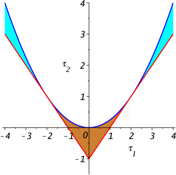
Figure 2: An illustration of the configuration space for $BC_{2}$ trigonometric model in $\tau$-variables (light brown area) and for $BC_{2}$ hyperbolic model (light blue area on the right).

As for $BC_{3}$

$$V_{BC_{3}}(\tau)=g\frac{\tau_{1}^{4}-\tau_{1}^{3}\tau_{3}-6\tau_{1}^{2}\tau_{2}+9\tau_{1}\tau_{2}\tau_{3}+9\tau_{2}^{2}-\tau_{2}^{3}-27\tau_{3}^{2}}{\tau_{1}^{2}\tau_{2}^{2}-4\tau_{1}^{3}\tau_{3}-4\tau_{2}^{2}-27\tau_{3}^{2}+18\tau_{1}\tau_{2}\tau_{3}}$$

$$\hphantom{V_{BC_{3}}(\tau)=}{}+\frac{g_{2}}{2}\frac{3+2\tau_{1}+\tau_{2}}{1+\tau_{1}+\tau_{2}+\tau_{3}}+\frac{g_{2}+4g_{3}}{4}\frac{3-2\tau_{1}+\tau_{2}}{1-\tau_{1}+\tau_{2}-\tau_{3}},$$ (2.38)

and

$$\Psi_{0}^{(BC_{3})}(\tau)=\big{(}\tau_{1}^{2}\tau_{2}^{2}-4\tau_{1}^{3}\tau_{3}-4\tau_{2}^{2}-27\tau_{3}^{2}+18\tau_{1}\tau_{2}\tau_{3}\big{)}^{\frac{\nu}{2}}$$

$$\hphantom{\Psi_{0}^{(BC_{3})}(\tau)=}{}\times(1+\tau_{1}+\tau_{2}+\tau_{3})^{\frac{\nu_{2}}{2}}(1-\tau_{1}+\tau_{2}-\tau_{3})^{\frac{\nu_{2}+\nu_{3}}{2}}.$$

The Hamiltonian (2.32) is completely-integrable: there exists a commutative algebra of integrals (including the Hamiltonian) of dimension $N$ which is equal to the dimension of the configuration space (for integrals, see Oshima [14] with explicit forms of those). Each integral ${\cal I}_{k}$ has a form polynomial in momentum of degree $2k\leq 2N$. Making gauge rotation with $\Psi_{0}^{2}$ and changing variable to (2.26) any integral appears in a form differential operator with polynomial coefficients. Evidently, it preserves the flag of polynomials (2.30) and can be written as a non-linear combination of the generators (2.29) at $d=N$ from its affine subalgebra. The explicit formulae of integrals in generators (2.29) are unknown. The spectra of the integral which is a polynomial in momentum of degree $2k$ is given by a polynomial in quantum numbers of the degree $2k$. All eigenfunctions of the integrals are common.

It is evident that for the $BC_{N}$ trigonometric model there exists a particular integral – $\pi$-integral of zero grading (see [22])

$$i_{\rm par}^{(n)}(\tau)=\prod_{j=0}^{n}\big{(}{\cal J}^{0}_{n}+j\big{)}$$

(cf. (2.31)), such that

$$\big{[}h_{BC_{N}}(\tau),i_{\rm par}^{(n)}(\tau)\big{]}:\ {\cal P}^{(N)}_{n}\mapsto 0.$$

Making the gauge rotation of the $\pi$-integral (2.31) with $\Psi_{0}^{-1}(\tau)$ given by (2.33) and changing variables $\tau$ (see (2.34)) back to the Cartesian coordinates we arrive at the quantum $\pi$-integral,

$${\cal I}_{{\rm par},BC_{N}}^{(n)}(x)=\Psi_{0}(\tau)i_{\rm par}^{(n)}(\tau)\Psi_{0}^{-1}(\tau)\big{|}_{\tau\rightarrow x}.$$

It is a differential operator of the $(n+1)$th order.

Under such a gauge transformation the triangular space of polynomials ${\cal P}^{(N)}_{n}$ becomes the space

$${\cal V}^{(N)}_{n}=\Psi_{0}{\cal P}^{(N)}_{n}.$$

The Hamiltonian ${\cal H}_{BC_{N}}(x)$ commutes with ${\cal I}_{{\rm par},BC_{N}}^{(n)}(x)$ over this space

$$\big{[}{\cal H}_{BC_{N}}(x),{\cal I}_{{\rm par},BC_{N}}^{(n)}(x)\big{]}:\ {\cal V}^{(N)}_{n}\mapsto 0.$$

Any eigenfunction $\Psi\in{\cal V}^{(N)}_{n}$ is zero mode of the $\pi$-integral ${\cal I}_{{\rm par},BC_{N}}^{(n)}(x)$.

Now we are in a position to draw an intermediate conclusion about $A_{N}$ and $BC_{N}$ trigonometric models.

• Both $A_{N}$- and $BC_{N}$-trigonometric (and rational) models possess algebraic forms associated with preservation of the same flag of polynomials ${\cal P}^{(N)}$. The flag is invariant with respect to linear transformations in space of orbits $\tau\mapsto\tau+A$. It preserves the algebraic form of Hamiltonian.

• Their Hamiltonians (as well as higher integrals) can be written in the Lie-algebraic form

  $$h=\operatorname{Pol}_{2}({\cal J}(b\subset gl_{N+1})),$$

  where $\operatorname{Pol}_{2}$ is a polynomial of 2nd degree in generators ${\cal J}$ of the maximal affine subalgebra of the algebra $b$ of the algebra $gl_{N+1}$ in realization (2.29). Hence, $gl_{N+1}$ is their hidden algebra. From this viewpoint all four models are different faces of a single model.

• Supersymmetric $A_{N}$- and $BC_{N}$-rational $($and trigonometric$)$ models possess algebraic forms, preserve the same flag of $($super$)$polynomials and their hidden algebra is the superalgebra $gl(N+1|N)$ $($see [4]).

In a connection to flags of polynomials we introduce a notion ‘characteristic vector’. Let us consider a flag made out of “triangular” linear space of polynomials

$${\cal P}^{(d)}_{n,\vec{f}}=\langle x_{1}^{p_{1}}x_{2}^{p_{2}}\cdots x_{d}^{p_{d}}\,|\,0\leq f_{1}p_{1}+f_{2}p_{2}+\cdots+f_{d}p_{d}\leq n\rangle,$$

where the “grades” $f$’s are positive integer numbers and $n=0,1,2,\ldots$. In lattice space ${\cal P}^{(d)}_{n,\vec{f}}$ defines a Newton pyramid.

Definition 2.1.

Characteristic vector is a vector with components $f_{i}$:

$$\vec{f}=(f_{1},f_{2},\ldots,f_{d}).$$

From geometrical point of view $\vec{f}$ is normal vector to the base of the Newton pyramid. The characteristic vector for flag ${\cal P}^{(d)}$ is

$$\vec{f}_{0}=\underbrace{(1,1,\ldots,1)}_{d}.$$

2.6 Case $\boldsymbol{G_{2}}$

Take the Hamiltonian

$${\cal H}_{G_{2}}=-\frac{1}{2}\sum_{k=1}^{3}\frac{\partial^{2}}{\partial x_{k}^{2}}+\frac{g\beta^{2}}{4}\sum_{k<l}^{3}\frac{1}{\sin^{2}(\frac{\beta}{2}(x_{k}-x_{l}))}+\frac{g_{1}\beta^{2}}{4}\sum_{k<lk,\,l\neq m}^{3}\frac{1}{\sin^{2}(\frac{\beta}{2}(x_{k}+x_{l}-2x_{m}))},$$

where $g$, $g_{1}$ and $\beta$ are parameters. It describes a trigonometric generalization of the rational Wolfes model of three-body interacting system or, in the Hamiltonian reduction nomenclature, the $G_{2}$-trigonometric model [13]. The symmetry of the model is dihedral group $D_{6}\oplus T$. The ground state function is

$$\Psi_{0}=\prod_{i<j}^{3}\left|\sin\frac{\beta}{2}(x_{i}-x_{j})\right|^{\nu}\prod_{k<lk,\,l\neq m}^{3}\left|\sin\frac{\beta}{2}(x_{i}+x_{j}-2x_{k})\right|^{\mu}$$

with $\nu,\mu>-\frac{1}{2}$ as solutions of

$$g=\nu(\nu-1)>-\frac{1}{4},\qquad g_{1}=3\mu(\mu-1)>-\frac{3}{4}.$$

Making the gauge rotation

$$h_{{G}_{2}}=(\Psi_{0})^{-1}({\cal H}_{G_{2}}-E)\Psi_{0},$$

and changing variables [15]

$$Y=\sum x_{i},\qquad y_{i}=x_{i}-\frac{1}{3}Y,\quad i=1,2,3,\qquad(x_{1},x_{2},x_{3})\rightarrow\big{(}Y,\tau_{1},\tau_{2}\big{)},$$

where

$$\tau_{1}=2[\cos(\beta(y_{1}-y_{2}))+\cos(\beta(2y_{1}+y_{2}))+\cos(\beta(y_{1}+2y_{2}))],$$

$$\tau_{2}=2[\cos(3\beta y_{1})+\cos(3\beta y_{2})+\cos(3\beta(y_{1}+y_{2}))]$$

are $G_{2}$ trigonometric invariants, and separating the center-of-mass coordinate we arrive at [15]

$$h_{G_{2}}=-\left(4+\tau_{1}+\frac{\tau_{2}}{3}-\frac{\tau_{1}^{2}}{3}\right)\partial_{\tau_{1}\tau_{1}}^{2}+\big{(}12+4\tau_{2}+\tau_{1}\tau_{2}-2\tau_{1}^{2}\big{)}\partial_{\tau_{1}\tau_{2}}^{2}$$

$$\hphantom{h_{\rm G_{2}}=}{}+\big{(}9\tau_{1}+3\tau_{2}+3\tau_{1}\tau_{2}+\tau_{2}^{2}-\tau_{1}^{3}\big{)}\partial_{\tau_{2}\tau_{2}}^{2}+\left[2\nu+\frac{1+3\mu+2\nu}{3}\tau_{1}\right]\partial_{\tau_{1}}$$

$$\hphantom{h_{\rm G_{2}}=}{}+\big{[}6\mu+(1+2\mu+\nu)\tau_{2}+2\nu\tau_{1}\big{]}\partial_{\tau_{2}},$$ (2.39)

which is the algebraic form of the $G_{2}$ trigonometric Hamiltonian. The eigenvalues of $h_{G_{2}}$ are

$$\epsilon_{\{p\}}=\frac{p_{1}^{2}}{3}+p_{1}p_{2}+p_{2}^{2}+(\mu+\nu)p_{1}+(2\mu+\nu)p_{2}$$

quadratic in quantum numbers $p_{1},p_{2}=0,1,2,\ldots$.

The Hamiltonian $h_{G_{2}}$ has infinitely many finite-dimensional invariant subspaces

$${\cal P}_{n,(1,2)}^{(2)}=\langle{\tau_{1}}^{p_{1}}{\tau_{2}}^{p_{2}}\,|\,0\leq p_{1}+2p_{2}\leq n\rangle,\qquad n=0,1,2,\ldots,$$ (2.40)

hence the flag ${\cal P}^{(2)}_{(1,2)}$ with the characteristic vector $\vec{f}=(1,2)$ is preserved by $h_{G_{2}}$. The eigenfunctions of $h_{G_{2}}$ are are elements of the flag ${\cal P}^{(2)}_{(1,2)}$. Each space $({\cal P}_{n,(1,2)}^{(2)}\ominus{\cal P}_{n-1,(1,2)}^{(2)})$ contains ${\sim}n$ eigenfunctions which is equal to length of the Newton line ${\cal L}_{n}=\langle{\tau_{1}}^{p_{1}}{\tau_{2}}^{p_{2}}|p_{1}+2p_{2}=n\rangle$.

A natural question to ask whether does an algebra of differential operators exist for which ${\cal P}_{n,(1,2)}^{(2)}$ is the space of (irreducible) representation. We call this algebra $g^{(2)}$ [15].

2.7 Algebra $\boldsymbol{g^{(2)}}$

Let us consider the Lie algebra spanned by seven generators

$$J^{1}=\partial_{t},\qquad J^{2}_{n}=t\partial_{t}-\frac{n}{3},\qquad J^{3}_{n}=2u\partial_{u}-\frac{n}{3},\qquad J^{4}_{n}=t^{2}\partial_{t}+2tu\partial_{u}-nt,$$

$$R_{i}=t^{i}\partial_{u},\quad i=0,1,2,\qquad{\cal R}^{(2)}\equiv(R_{0},R_{1},R_{2}).$$ (2.41)

It is non-semi-simple algebra $gl(2,{\mathbb{R}})\ltimes{\cal R}^{(2)}$ (S. Lie [11, p. 767–773] at $n=0$ and A. González-Lopéz et al. [9] at $n\neq 0$ (case 24)). If the parameter $n$ in (2.41) is a non-negative integer, it has (2.40)

$${\cal P}_{n}^{(2)}=\big{(}t^{p}u^{q}\,|\,0\leq(p+2q)\leq n\big{)},$$

as common (reducible) invariant subspace. By adding three operators

$$T_{0}=u\partial_{t}^{2},\qquad T_{1}=u\partial_{t}J_{0}^{(n)},\qquad T_{2}=uJ_{0}^{(n)}\big{(}J_{0}^{(n)}+1\big{)}=uJ_{0}^{(n)}J_{0}^{(n-1)},$$ (2.42)

where

$$J_{0}^{(n)}=t\partial_{t}+2u\partial_{u}-n,$$

to $gl(2,{\mathbb{R}})\ltimes{\cal R}^{(2)}$ (see (2.41)), the action on ${\cal P}_{n,(1,2)}^{(2)}$ gets irreducible. Multiple commutators of $J^{4}_{n}$ with $T_{0}^{(2)}$ generate new operators acting on ${\cal P}_{n,(1,2)}^{(2)}$,

$$T_{i}\equiv\underbrace{[J^{4},[J^{4},[\ldots J^{4},T_{0}]\ldots]}_{i}=u\partial_{t}^{2-i}J_{0}^{(n)}\big{(}J_{0}^{(n)}+1\big{)}\cdots(J_{0}^{(n)}+i-1)$$

$$\hphantom{T_{i}\equiv\underbrace{[J^{4},[J^{4},[\ldots J^{4},T_{0}]\ldots]}_{i}}{}=u\partial_{t}^{2-i}\prod_{j=0}^{i-1}J_{0}^{(n-j)},\qquad i=0,1,2,$$

all of them are differential operators of degree $2$. These new generators have a property of nilpotency,

$$T_{i}=0,\qquad i>2,$$

and commutativity:

$$[T_{i},T_{j}]=0,\qquad i,j=0,1,2,\quad{\cal U}^{(2)}\equiv(T_{0},T_{1},T_{2}).$$

The generators (2.41) plus (2.42) span a linear space with a property of decomposition: $g^{(2)}\doteq{\cal R}^{(2)}\rtimes(gl_{2}\oplus J_{0})\ltimes{\cal U}^{(2)}$ (see Fig. 3).

Figure 3: Triangular diagram relating the subalgebras $L$, $U$ and $g\ell_{2}$. ${P}_{2}{(g\ell_{2})}$ is a polynomial of the 2nd degree in $g\ell_{2}$ generators. It is a generalization of the Gauss decomposition for semi-simple algebras.

It is worth mentioning a property of conjugation ${\cal R}^{(2)}\Leftrightarrow{\cal T}^{(2)}$:

$$\partial_{\tau_{2}}\leftrightarrow{\tau_{2}}J_{0}^{(n)}\big{(}J_{0}^{(n)}+1\big{)},\qquad{\tau_{1}}\partial_{\tau_{2}}\leftrightarrow{\tau_{2}}\partial_{\tau_{1}}J_{0}^{(n)},\qquad{\tau_{1}}^{2}\partial_{\tau_{2}}\leftrightarrow{\tau_{2}}\partial_{\tau_{1}}^{2}.$$

where $J_{0}^{(n)}={\tau_{1}}\partial_{\tau_{1}}+2{\tau_{2}}\partial_{\tau_{2}}-n$.

Eventually, infinite-dimensional, eleven-generated algebra $($by (2.41) and $J_{0}$ plus (2.42), so that the eight generators are the $1$st order and three generators are of the $2$nd order differential operators$)$ occurs. The Hamiltonian $h_{G_{2}}$ can be rewritten in terms of the generators (2.41), (2.42) with the absence of the highest weight generator $J^{4}_{n}$,

$$h_{G_{2}}=-\big{(}4J^{1}+J^{2}-2J^{3}-12R_{0}+2R_{2}\big{)}J^{1}+\frac{1}{6}\big{(}2J^{2}+3J^{3}\big{)}J^{2}+\left(J^{3}+\frac{3}{2}R_{1}\right)J^{3}$$

$$\hphantom{h_{G_{2}}=}{}+(9R_{0}-R_{2})R_{1}-\frac{1}{3}T_{0}+2\nu J^{1}+\frac{3\mu\!+\!2\nu}{3}J^{2}+\frac{2\mu\!+\!\nu\!-\!1}{2}J^{3}+6\mu R_{0}+\left(2\nu-\frac{3}{2}\right)R_{1}$$

(see [15]), where $J^{2,3}\equiv J^{2,3}_{0}$. Hence, $gl(2,{\mathbb{R}})\ltimes{\cal R}^{(2)}$ is the hidden algebra of the $G_{2}$ trigonometric model.

The $G_{2}$ trigonometric Hamiltonian admits the integral in a form of the 6th order differential operator [14]. After gauge rotation with $\Psi_{0}$ in variables $\tau_{1,2}$ the integral has to take the algebraic form which is not known explicitly. This integral preserves the same flag ${\cal P}^{(2)}_{(1,2)}$ as the Hamiltonian (2.39). It can be rewritten in term of generators of the algebra $g^{(2)}$. In addition to it, there exists $\pi$-integral of zero grading (see [22])

$$i_{\rm par}^{(n)}(\tau)=\prod_{j=0}^{n}\big{(}J_{0}^{(n)}+j\big{)}=\prod_{j=0}^{n}J_{0}^{(n-j)}$$

(cf. (2.31)), such that

$$\big{[}h_{G_{2}}(\tau),i_{\rm par}^{(n)}(\tau)\big{]}:\ {\cal P}_{n,(1,2)}^{(2)}\mapsto 0.$$

Making the gauge rotation of the $\pi$-integral (2.31) with $\Psi_{0}^{-1}(\tau)$ given by (2.33) and changing variables $\tau$ (see (2.34)) back to the Cartesian coordinates we arrive at the quantum $\pi$-integral,

$${\cal I}_{{\rm par},G_{2}}^{(n)}(x)=\Psi_{0}(\tau)i_{\rm par}^{(n)}(\tau)\Psi_{0}^{-1}(\tau)\big{|}_{\tau\rightarrow x}.$$

It is a differential operator of the $(n+1)$th order.

Under such a gauge transformation the triangular space of polynomials ${\cal P}_{n,(1,2)}^{(2)}$ becomes the space

$${\cal V}^{(N)}_{n}=\Psi_{0}{\cal P}_{n,(1,2)}^{(2)}.$$

The Hamiltonian ${\cal H}_{G_{2}}(x)$ commutes with ${\cal I}_{{\rm par},G_{2}}^{(n)}(x)$ over this space

$$\big{[}{\cal H}_{G_{2}}(x),{\cal I}_{{\rm par},G_{2}}^{(n)}(x)\big{]}:\ {\cal V}^{(N)}_{n}\mapsto 0.$$

Any eigenfunction $\Psi\in{\cal V}^{(N)}_{n}$ is zero mode of the $\pi$-integral ${\cal I}_{{\rm par},G_{2}}^{(n)}(x)$.

Summarizing let us mention that in addition to the flag ${\cal P}^{(2)}_{(1,2)}$ the $G_{2}$ trigonometric Hamiltonian preserves two more flags: ${\cal P}_{(3,5)}$ and ${\cal P}_{(5,9)}$, where their characteristic vectors $(3,5)$ and $(5,9)$ coincide to the Weyl vector and co-vector, respectively.

2.8 Cases $\boldsymbol{F_{4}}$ and $\boldsymbol{E_{6,7}}$

These three cases are described in some details in [2, 12] and in [3, p. 1416], respectively.

2.9 Case $\boldsymbol{E_{8}}$ (in brief)

In this Section a brief description of $E_{8}$ trigonometric case is given, all details can be found in [3].

The $E_{8}$ trigonometric Hamiltonian has a form (1.2),

$$\mathcal{H}_{E_{8}}\left(\frac{\beta}{2}\right)=-\frac{1}{2}\Delta^{(8)}+\frac{g\beta^{2}}{4}\sum_{j<i=1}^{8}\left[\frac{1}{\sin^{2}{\frac{\beta}{2}(x_{i}+x_{j})}}+\frac{1}{\sin^{2}{\frac{\beta}{2}(x_{i}-x_{j})}}\right]$$

$$\hphantom{\mathcal{H}_{E_{8}}\left(\frac{\beta}{2}\right)=}{}+\frac{g\beta^{2}}{4}\sum_{\{\nu_{j}\}}\frac{1}{\Big{[}\sin^{2}\frac{\beta}{4}\Big{(}{x_{8}+\sum\limits_{j=1}^{7}(-1)^{\nu_{j}}x_{j}}\Big{)}\Big{]}},$$ (2.43)

and it acts in ${\mathbb{R}}^{8}$. The second summation being one over septuples $\{\nu_{j}\}$ where each $\nu_{j}=0,1$ and $\sum\limits_{j=1}^{7}\nu_{j}$ is even. Here $g=\nu(\nu-1)>-1/4$ is the coupling constant and $\beta$ is a parameter. The configuration space is the principal $E_{8}$ Weyl alcove. Symmetry of the $E_{8}$ trigonometric model is given by the affine ${\rm E_{8}}$ Weyl group of the order 696 729 600. The ground state function $\Psi_{0}$ is given by (1.3). Making a gauge rotation of the Hamiltonian

$$h_{E_{8}}=\frac{1}{\beta^{2}}(\Psi_{0})^{-1}(\mathcal{H}_{E_{8}}-E_{0})\Psi_{0},$$

where $E_{0}=310\beta^{2}\nu^{2}$ is the ground state energy, and introducing the new variables $\tau_{1,\ldots,8}(\beta)$, which are the fundamental trigonometric invariants with respect to the ${\rm E_{8}}$ Weyl group, we arrive at the $E_{8}$ trigonometric Hamiltonian in the algebraic form

$$h_{E_{8}}=\sum_{i,j=1}^{4}A_{ij}(\tau)\frac{\partial^{2}}{\partial\tau_{i}\partial\tau_{j}}+\sum_{j=1}^{4}B_{j}(\tau,\nu)\frac{\partial}{\partial\tau_{j}},$$ (2.44)

where $A_{ij}(\tau)$, $B_{j}(\tau;\nu)$ are polynomials in $\tau$ with integer coefficients and $B_{j}(\tau;\nu)$ depend on $\nu$ linearly (see [3, Appendix A]).

It is easy to check that the algebraic operator $h_{E_{8}}$ has infinitely-many finite-dimensional invariant subspaces

$$\mathcal{P}_{n}^{(2,2,3,3,4,4,5,6)}=\langle\tau_{1}^{n_{1}}\tau_{2}^{n_{2}}\tau_{3}^{n_{3}}\tau_{4}^{n_{4}}\tau_{5}^{n_{5}}\tau_{6}^{n_{6}}\tau_{7}^{n_{7}}\tau_{7}^{n_{8}}\,|$$

$$\hphantom{\mathcal{P}_{n}^{(2,2,3,3,4,4,5,6)}=\langle}{}0\leq 2n_{1}+2n_{2}+3n_{3}+3n_{4}+4n_{5}+4n_{6}+5n_{7}+6n_{8}\leq n\rangle,\qquad n\in\mathbb{N},$$

all of them have with the same characteristic vector $\vec{f}=(2,2,3,3,4,4,5,6)$, they form the infinite flag. The spectrum of the Hamiltonian $h_{E_{8}}$ (2.44) is quadratic in quantum numbers [3, 10].

Eigenfunctions $\phi_{n,\{p\}}$ of $h_{E_{8}}$ are elements of $\mathcal{P}_{n}^{(2,2,3,3,4,4,5,6)}$. The number of eigenfunctions in $\mathcal{P}_{n}^{{(2,2,3,3,4,4,5,6)}}$ is equal to the dimension of $\mathcal{P}_{n}^{{(2,2,3,3,4,4,5,6)}}$.

The space $\mathcal{P}^{{(2,2,3,3,4,4,5,6)}}_{n}$ is a finite-dimensional representation space of a Lie algebra of differential operators which we call the $e^{(8)}$ algebra [6]. It is infinite-dimensional but finitely generated algebra of differential operators, with 968 generating elements in a form of differential operators of the orders $1^{\text{st}}$ (54), $2^{\text{nd}}$ (24), $3^{\text{rd}}$ (18), $4^{\text{rd}}$ (18), $5^{\text{rd}}$ (28), $6^{\text{rd}}$ (5) plus one of zeroth order (constant). They span 100 + 100 Abelian (conjugated) subalgebras of lowering and raising generators $L$ and $U$ and one algebra $B$ of the Cartan type of dimension 15 plus one central element. Among the generators of $B$ there is the Euler–Cartan operator

$$J_{0}^{(n)}=2\tau_{1}\partial_{\tau_{1}}+2\tau_{2}\partial_{\tau_{2}}+3\tau_{3}\partial_{\tau_{3}}+3\tau_{4}\partial_{\tau_{4}}+4\tau_{5}\partial_{\tau_{5}}+4\tau_{6}\partial_{\tau_{6}}+5\tau_{7}\partial_{\tau_{7}}+6\tau_{8}\partial_{\tau_{8}}-n.$$ (2.45)

Taking the algebra $B$ and a pair of conjugated Abelian algebras one can show that the commutation relations lead to the diagram of Fig. 4. Depending on what pair $L$, $U$ the degree $p$ takes the following values: 2, 3, 4, 5, 6, 7, 8, 9, 10.

Figure 4: Triangular diagram relating the subalgebras $L$, $U$ and $B$. ${P}_{p}{(B)}$ is a polynomial of the $p$th degree in $B$ generators. It is a generalization of the Gauss decomposition for semi-simple algebras.

The $E_{8}$ trigonometric model is completely-integrable – there exist seven algebraically independent mutually commuting differential operators of finite order that commute with the Hamiltonian (2.43) [10, 13]. We are not aware on the existence of their explicit forms. It seems evident that any of these integrals after the gauge rotation with the ground state function $\Psi_{0}$ the space of orbits should take an algebraic form of a differential operator with polynomial coefficient functions. Any integral as well as the Hamiltonian is an element of the algebra $e^{(8)}$. In addition to “global” integrals, there exists $\pi$-integral of zero grading (see [22])

$$i_{\rm par}^{(n)}(\tau)=\prod_{j=0}^{n}\big{(}J_{0}^{(n)}+j\big{)}=\prod_{j=0}^{n}J_{0}^{(n-j)},$$

where $J_{0}^{(n)}$ is given by (2.45) (cf. (2.31)) such that

$$\big{[}h_{E_{8}}(\tau),i_{\rm par}^{(n)}(\tau)\big{]}:\ \mathcal{P}_{n}^{(2,2,3,3,4,4,5,6)}\mapsto 0.$$

It is worth mentioning that the operator (2.44) has a certain property of degeneracy: it also preserves the infinite flag of the spaces of polynomials with the characteristic vector $\vec{f}=(29,46,57,68,84,91,110,135)$. This vector coincides to the $E_{8}$ Weyl (co)vector. Hence, the eigenfunctions of $h_{E_{8}}(\tau)$ are the elements of this flag as well. It implies the existence of another $\pi$-integral $\tilde{i}_{\rm par}^{(n)}(\tau)$ with $J_{0}^{(n)}$ given by

$$J_{0}^{(n)}=29\tau_{1}\partial_{\tau_{1}}\!+46\tau_{2}\partial_{\tau_{2}}\!+57\tau_{3}\partial_{\tau_{3}}\!+68\tau_{4}\partial_{\tau_{4}}\!+84\tau_{5}\partial_{\tau_{5}}\!+91\tau_{6}\partial_{\tau_{6}}\!+110\tau_{7}\partial_{\tau_{7}}\!+135\tau_{8}\partial_{\tau_{8}}\!-n,$$

such that

$$\big{[}h_{E_{8}}(\tau),\tilde{i}_{\rm par}^{(n)}(\tau)\big{]}:\ \mathcal{P}_{n}^{(29,46,57,68,84,91,110,135)}\mapsto 0.$$

3 Conclusions

• For trigonometric Hamiltonians for all classical $A_{N}$, $BC_{N}$, $B_{N}$, $C_{N}$, $D_{N}$ and for exceptional root spaces $G_{2}$, $F_{4}$, $E_{6,7,8}$, similar to the rational Hamiltonians including non-crystallographic $H_{3,4}$, $I_{2}(k)$ (see [21]), there exists an algebraic form after gauging away the ground state eigenfunction, and changing variables from Cartesian to fundamental trigonometric Weyl invariants (see [1, 2, 3, 4, 12, 15, 16]). Their eigenfunctions are polynomials in these variables. They are orthogonal with respect to the squared ground state eigenfunction.

  Coefficient functions in front of the second derivatives of these gauge-rotated Hamiltonians which are polynomials in fundamental trigonometric Weyl invariants define a metric ${\cal A}$ of flat space in the space of orbits. We will call this metric the V.I. Arnold metric, he was the first to calculate a similar metric in the case of polynomial Weyl invariants. This metric has a property that in the Laplace–Beltrami operator the coefficient functions in front of the first derivatives are polynomials in fundamental trigonometric invariants. This property is similar to one which occurs in the case of rational models. The (rational) Arnold metric for the space of orbits parameterized by polynomial Weyl invariants can be considered as an appropriate degeneration of the (trigonometric) Arnold metric for the space of orbits parameterized by fundamental trigonometric Weyl invariants.

• Any trigonometric Hamiltonian is characterized by a hidden algebra. These hidden algebras are $U_{gl(N+1)}$ for the case of classical $A_{N}$, $BC_{N}$, $B_{N}$, $C_{N}$, $D_{N}$ and new infinite-dimensional but finite-generated algebras of differential operators for all other cases. All these algebras have finite-dimensional invariant subspace(s) in polynomials. Rational Hamiltonians are characterized by the same hidden algebra with a single exception of the $E_{8}$ case.

• The generating elements of any such hidden algebra can be grouped into an even number of (conjugated) Abelian algebras $L_{i}$, $U_{i}$ and one Lie algebra $B$. They obey a (generalized) Gauss decomposition rule (see Fig. 5). A study and a description of all these algebras is in progress and will be given elsewhere.

  

  Figure 5: Triangular diagram relating the subalgebras $L$, $U$ and $B$. ${P}_{p}{(B)}$ is a polynomial of the $p$th degree in $B$ generators. It is a generalization of the Gauss decomposition for semi-simple algebras where $p=1$.

  Table 1: Minimal characteristic vectors for rational (non)crystallographic and trigonometric crystallographic systems (see [3]). For latter case the Weyl vector and co-vector as possible characteristic vectors occur. Characteristic vectors for $H_{3}$, $H_{4}$, $I_{2}(k)$ are from [7, 8, 19], respectively.

  Model	Rational	Trigonometric
  		minimal	integer Weyl	integer co-Weyl
  $A_{N}$2pt	$\underbrace{(1,1,\ldots,1)}_{N}$6pt	$\underbrace{(1,1,\ldots,1)}_{N}$
  $BC_{N}$2pt	$\underbrace{(1,1,\ldots,1)}_{N}$	$\underbrace{(1,1,\ldots,1)}_{N}$
  $G_{2}$	(1,2)	(1,2)	(3,5)	$(5,9)$
  $F_{4}$	(1,2,2,3)	(1,2,2,3)	(8,11,15,21)	(11,16,21,30)
  $E_{6}$	(1,1,2,2,2,3)	(1,1,2,2,2,3)	(8,8,11,15,15,21)	(8,8,11,15,15,21)
  $E_{7}$	(1,2,2,2,3,3,4)	(1,2,2,2,3,3,4)	$(27,34,49,52,66,75,96)$	$(27,34,49,52,66,75,96)$
  $E_{8}$	(1,3,5,5,7,7,9,11)	(2,2,3,3,4,4,5,6)	(29,46,57,68,84,91,110,135)	(29,46,57,68,84,91,110,135)
  $H_{3}$	(1,2,3)	—
  $H_{4}$	(1,5,8,12)	—
  $I_{2}(k)$	$(1,k)$	—

• Any algebraic Hamiltonian $h$ of a trigonometric model preserves one or several flags of invariant subspaces with characteristic vectors given by the highest root vector, the Weyl vector and the Weyl co-vector (see Table 1). With the single exception of the $E_{8}$ case the flags for rational and trigonometric models coincide.

• The original Weyl-invariant periodic Hamiltonian (1.1) written in the fundamental trigonometric invariants (2.1) corresponds to a particle moving in flat space with (trigonometric) Arnold metric ${\cal A}$ in a rational potential,

  $${\cal H}(\tau)=-\Delta_{\cal A}+\sum^{\ell}_{k}g_{k}V_{k}(\tau),$$

  where $\Delta_{\cal A}$ is the Laplace–Beltrami operator, $g_{k}$, $k=1,\ldots,\ell$ are coupling constants, $\ell$ is the number of different root lengths in the root space. $V_{k}(\tau)$ are rational functions. So far, we are unaware about the explicit form of the functions $V_{k}(\tau)$ for all root systems except for some particular cases (see (2.7), (2.21), (2.37), (2.38)).

• The existence of an algebraic form of the Hamiltonian $h$ of a trigonometric model allows us to construct integrable discrete systems in the space of orbits with the same hidden algebra structure, having a property of isospectrality, on uniform, exponential and mixed uniform-exponential lattices following the strategy presented in [17] (uniform lattice) and [5] (exponential lattice).

• The space of orbits formalism allowed us to show that both rational and trigonometric models for any root system are essentially algebraic: the (appropriately) gauge-rotated Hamiltonians are algebraic operators, their invariant subspaces are spaces of polynomials. A natural question to ask is: How the elliptic Calogero–Moser systems look like in a space of orbits formalism; are they algebraic just like rational and trigonometric systems? A main obstruction to get an answer is that, in general, it is not known how to construct elliptic invariants – the invariants with respect to a “double”-affine Weyl group (the Weyl group plus two translations) – on a regular basis. However, such invariants can be constructed explicitly for two particular root systems: $A_{1}/BC_{1}$ [24] and $BC_{2}$ [20]. It can be shown that the corresponding elliptic systems are algebraic.

Acknowledgements

This work was supported in part by the University Program FENOMEC, by the PAPIIT grant IN109512 and CONACyT grant 166189 (Mexico).