Co-circulation of infectious diseases on networks

Abstract

We consider multiple diseases spreading in a static Configuration Model network. We make standard assumptions that infection transmits from neighbor to neighbor at a disease-specific rate and infected individuals recover at a disease-specific rate. Infection by one disease confers immediate and permanent immunity to infection by any disease. Under these assumptions, we find a simple, low-dimensional ordinary differential equations model which captures the global dynamics of the infection. The dynamics depend strongly on initial conditions. Although we motivate this article with infectious disease, the model may be adapted to the spread of other infectious agents such as competing political beliefs, rumors, or adoption of new technologies if these are influenced by contacts. As an example, we demonstrate how to model an infectious disease which can be prevented by a behavior change.

Introduction

Networks have captured the attention of many scientists. One of the primary interests is in understanding how network structure governs the behavior of dynamic processes spreading on networks larremore:neuronal ; durrett:vote ; pastor-satorras:dynamics . This is complicated by difficulty in deriving analytic models, limiting our understanding of the dynamics. Sometimes we can gain insight into long-term behavior without understanding dynamics, but in many cases the intermediate dynamics governs the long-term outcome. This is particularly significant when competing processes are occurring in the network. In this article we study the simultaneous spread of two competing diseases in a Configuration Model network. Although we focus on disease, other competing “infectious” processes, such as a change in behavior in response to a disease funk:behavior , spread of beliefs in a voter model durrett:vote , and “viral marketing” of competing technologies bharathi:competing_tech have been studied, and the approach introduced here can be adapted to these applications.

In this article we derive a low-dimensional system of equations capturing the dynamics of competing diseases spreading simultaneously in a Configuration Model network. We apply the model to investigating possible outcomes of co-circulating diseases. Prior studies have thoroughly analyzed the effect of network structure such as degree distribution newman:spread ; pastor-satorras:scale-free ; boguna:scalefree ; may:dynamics and heterogeneities in infectiousness and/or susceptibility miller:heterogeneity ; miller:bounds ; kenah:second ; trapman:analytical on disease spread. Recent work gives insight into the role of partnership duration volz:dynamic_network ; miller:ebcm_overview ; miller:ebcm_structure ; miller:ebcm_hierarchy . Other investigations focus on the role of clustering miller:RSIcluster ; miller:random_clustered ; newman:cluster_alg ; gleeson:clustering_effect ; melnik:unreasonable ; volz:clustered_result ; house:insights ; trapman:analytical ; eames:clustered , with limited predictive success.

Models of interacting diseases typically neglect network structure (e.g., andreasen:cocirculate ; cobey:competition and many others). Until recently, models of a single disease spreading through a network have relied on approximation eames:pair or been restricted to final size calculations under the assumption of an asymptotically small initial fraction infected newman:spread . Extending these approaches to competing diseases newman:threshold ; karrer:competing ; funk:interacting does not allow us to measure the effect of dynamic interactions, and so results are limited to special cases in which these interactions are not important, such as when one disease spreads before the other.

Our method can be easily adapted to more than $2$ diseases and allows for arbitrarily large initial conditions. We validate the system by comparison with simulation. Using our equations, we are able to identify the scalings which separate different regimes. We discuss these regimes and introduce possible generalizations.

The basic model

We assume that two diseases spread in a Configuration Model network newman:structurereview (also called a Molloy-Reed network MolloyReed ) with degree distribution given by $P(k)$. For disease $1$ transmission along an edge has rate $\beta_{1}$ and recovery of infected individuals has rate $\gamma_{1}$. For disease $2$ the rates are $\beta_{2}$ and $\gamma_{2}$. A node infected by either disease gains immunity to any further infection.

Our approach is similar to that of karrer:message and is based on miller:ebcm_overview . We will focus our attention on a test individual $u$ (described more fully in the appendix and miller:final ), a randomly chosen individual in the population. We assume that the aggregate population-scale spread of the diseases is deterministic. Under these assumptions, the probability the test individual has a given infection status equals the proportion of the population with that status. Thus by calculating the probability a test individual has a given status, we immediately know the proportion of the population with that status.

We make one change to the test individual $u$: we prevent it from causing infections. This keeps the status of its partners independent of one another without affecting its own status, and so it has no effect on our calculations of the proportion of the population in each state. An alternate argument for why this change has no impact is that we have assumed the dynamics are deterministic, while the timing of when (or even if) $u$ is infected is a random variable. Thus the infections $u$ would cause cannot have any macroscopic impact on the disease dynamics, and this modification of $u$ has no effect.

We take $t=t_{0}$ to be our “initial time”. In practice this may correspond to the time of introduction of a disease if enough individuals are initially infected, or it corresponds to a later time at which enough infection is present that the spread is deterministic. There are some restrictions on how the initial infections can be distributed, discussed in the appendix. We choose a test individual $u$ randomly from the population (it may have any status). We let $v$ be a random neighbor of a random test individual $u$ which had not transmitted to $u$ by $t_{0}$. We define $\theta(t)$ to be the probability that at time $t$, $v$ has not transmitted to $u$. The probability $u$ is susceptible at time $t$ is

$$S(t)=\psi(\theta(t))=\sum_{k}P(k)S(k,t_{0})\theta(t)^{k}$$

where $S(k,t_{0})$ is the probability an individual of degree $k$ is susceptible at $t=t_{0}$. We take $I_{1}$ and $I_{2}$ [resp $R_{1}$ and $R_{2}$] to be the probabilities that $u$ is infected with [resp has recovered from] the corresponding disease.

To calculate the change of $\theta$, we must know more about the probability $v$ is in any given state. We define $\phi_{S}(t)$ to be the probability $v$ is susceptible, $\phi_{I,1}(t)$ and $\phi_{I,2}(t)$ to be the probabilities that $v$ is infected has not transmitted to $u$, and $\phi_{R}$ to be the probability $v$ is recovered but did not transmit (we do not need to distinguish which disease infected $v$). Then $\theta=\phi_{S}+\phi_{I,1}+\phi_{I,2}+\phi_{R}$.

We calculate $\phi_{S}$ similarly to $S$. If $v$ is initially susceptible we find the probability it has degree $k$ by counting all edges of initially susceptible individuals of degree $k$: $NkP(k)S(k,t_{0})$ and dividing by the number of all edges of initially susceptible individuals $\sum_{k}NkP(k)S(k,t_{0})$ ($N$ is population size). If $v$ has degree $k$ and was initially susceptible, the probability $v$ is still susceptible is $\theta^{k-1}$ (because $u$ is prevented from transmitting to $v$). This leads to the conclusion that $v$ is susceptible with probability $\phi_{S}(t)=\phi_{S}(t_{0})\frac{\sum_{k}kP(k)S(k,t_{0})\theta^{k-1}}{\sum_{k}kP(k)S(k,t_{0})}=\phi_{S}(t_{0})\frac{\psi^{\prime}(\theta)}{\psi^{\prime}(1)}$.

Figure 1: (left) flow diagram for the probabilities the test individual has each status. (right) flow diagram for the probabilities a partner of the test individual has each status.

Fig. 1 gives flow diagrams which yield our equations. Each box represents a compartment, and arrow labels represents probability flux from one compartment to another. The fluxes from the $I$ compartments to the $R$ compartments represent recovery of $u$. The fluxes from the $\phi_{I}$ compartments to the $\phi_{R}$ compartments [resp $1-\theta$] represent flux due to recovery of $v$ prior to transmitting [resp transmission prior to recovery]. The fluxes from $S$ and $\phi_{S}$ are found by differentiation of $S$ and $\phi_{S}$ in time, using $\dot{\theta}=-\beta_{1}\phi_{I,1}-\beta_{2}\phi_{I,2}$, and assigning the appropriate proportion to the appropriate compartment.

From the diagram, we find

$$\dot{\theta} =-\beta_{1}\phi_{I,1}-\beta_{2}\phi_{I,2}$$ (1)

$$\dot{\phi}_{I,m} =-(\beta_{m}+\gamma_{m})\phi_{I,m}+\beta_{m}\phi_{I,m}\phi_{S}(t_{0})\frac{\psi^{\prime\prime}(\theta)}{\psi^{\prime}(1)}$$ (2)

$$S =\psi(\theta)$$ (3)

$$\dot{I}_{m} =\beta_{m}\phi_{I,m}\psi^{\prime}(\theta)-\gamma_{m}I_{m}$$ (4)

$$\dot{R}_{m} =\gamma_{m}I_{m}$$ (5)

The subscript $m$ takes the values $1$ and $2$. The single-disease, small initial condition limit of these equations has been proved exact decreusefond:volz_limit . These equations capture the fact that disconnected components are safe from outside introduction.

Sequential Introduction

As an example, we consider two diseases spreading in a network of $10^{6}$ individuals with Poisson degree distribution of mean $5$. For both, $\gamma=1$ but $\beta_{1}=0.5$ and $\beta_{2}=1$. In simulations, we introduce disease $1$ into $30$ random individuals at $t=0$, and disease $2$ into $30$ random individuals at $t=5.25$.

Our deterministic equations do not apply while either disease has a small number of infections. We take observations at $t_{0}=4$ (after the first, but before the second disease) and $t_{0}=7$ (after both are established) to initialize our equations. Fig. 2 compares calculation with simulation. Comparing the $t_{0}=4$ calculation with the $t_{0}=7$ calculation shows the effect of the second disease.

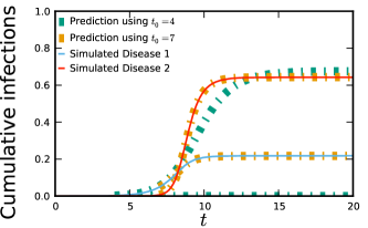
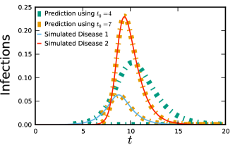
Figure 2: The spread of two diseases in a population of size $10^{6}$ with a Poisson degree distribution of mean $5$. The first disease is introduced with $30$ cases at $t=0$, and the second with $30$ cases at $t=5.25$. The second strain is more infectious. Predictions (dashed) are calculated from observations at $t=4$ (before the second disease’s introduction) and $t=7$ (shortly after). Model and simulation agree well.

Simultaneous Introduction

We now consider the simultaneous introduction of two diseases and assume that the initial numbers infected are large enough that the dynamics are deterministic. In our example, we take $\beta_{1}=1.2$,  $\gamma_{1}=4$,  $\beta_{2}=0.2$, and $\gamma_{2}=0.25$. Disease $1$ tends to spread more quickly, but disease $2$ has a higher probability of transmission prior to recovery. At $t=0$, we infected a randomly selected proportion of the population $\rho_{1}$ with disease $1$, and a proportion $\rho_{2}$ with disease $2$. This gives $S(k,0)=1-\rho_{1}-\rho_{2}$ for all $k$,  $I_{1}=\rho_{1}$,  $I_{2}=\rho_{2}$,  $\phi_{I,1}=\rho_{1}$, and $\phi_{I,2}=\rho_{2}$, with no recovered individuals. In our population, the degree of each node is assigned uniformly from the integers $1$ through $9$. We use our equations to calculate the final proportion infected by each disease, shown in Fig. 3.

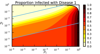
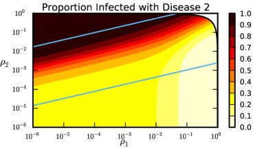
Figure 3: We take a network with the degree of each node chosen uniformly from $1$ up to $9$. A proportion $\rho_{1}$ of the population begins infected with disease $1$ and a proportion $\rho_{2}$ begins infected with disease $2$ with $\beta_{1}=1.2$,  $\gamma_{1}=4$,  $\beta_{2}=0.2$, and $\gamma_{2}=0.25$. Disease $1$ spreads more quickly, but has a smaller per-edge transmission probability. The solid lines denote the estimated upper and lower bounds of the overlapping epidemic regime.

There are several distinct regimes we can identify in Fig. 3. If $\rho_{2}$ is $\mathcal{O}(1)$ and $\rho_{1}$ small, or if $\rho_{1}$ is $\mathcal{O}(1)$ and $\rho_{2}$ small, the disease with the large initial condition spreads and effectively infects everyone simply because a large fraction is initially infected. The other disease cannot spread in the “residual network” left behind. If neither $\rho_{1}$ or $\rho_{2}$ is initially large, other regimes are seen. To analyze them, we first note that when both diseases are small, they grow at exponential rates $r_{1}=-(\beta_{1}+\gamma_{1})+\beta_{1}\psi^{\prime\prime}(1)/\psi^{\prime}(1)=2$ and $r_{2}=-(\beta_{2}+\gamma_{2})+\beta_{2}\psi^{\prime\prime}(1)/\psi^{\prime}(1)=0.75$.

In the “overlapping epidemic” regime, the slower-growing disease $2$ begins with a head start. The size of the head start scales so that the two epidemics become large at the same time. The value of $\ln I_{2}-(r_{2}/r_{1})\ln I_{1}$ is constant during the linear growth phase. For given $C=\ln\rho_{2}-(r_{2}/r_{1})\ln\rho_{1}$, the behavior is universal. The diseases grow independently until the linear growth phase ends. We can estimate bounds on the regime by crudely assuming exponential growth continues forever. There is some value of $C_{\text{min}}=\ln 0.0025-(r_{2}/r_{1})\ln 1=\ln 0.0025\approx-6$ that corresponds to $\rho_{1}=1$ and $\rho_{2}=0.0025$ which means that the slower growing disease would affect less than one percent of the population by the time the faster growing disease has fully established itself in this approximation. Similarly we take some $C_{\text{max}}=\ln 1-(r_{2}/r_{1})\ln 0.05=-(r_{2}/r_{1})\ln 0.05\approx 3r_{2}/r_{1}$ corresponding to $\rho_{1}=0.05$ and $\rho_{2}=1$, which means that the slower growing disease will have fully burned through the population when the faster growing disease is only affecting 5% of the population in this approximation. For $C<C_{\text{min}}$, $I_{1}$ becomes large well before $I_{2}$. For $C>C_{\text{max}}$, $I_{2}$ becomes large well before $I_{1}$. Between these values, the epidemics become large at similar times and interact dynamically. Further discussion of these boundaries is in the appendix.

There are two“non-overlapping epidemic” regimes. If $C<C_{\text{min}}$, disease $1$ becomes large and has an epidemic while disease $2$ is still exponentially small. If $C>C_{\text{max}}$, disease $2$ has an epidemic while disease $1$ is still exponentially small. Once one epidemic has finished, it may be possible for the remaining disease to spread in the residual network. We can derive the threshold condition: For simplicity we assume disease $1$ spreads first. While it spreads, $\phi_{I,2}$ remains negligible. By looking at the relative fluxes out of $\phi_{I,1}$ we conclude that after disease $1$ has completed its spread but before disease $2$ is significant, $\phi_{R}=\gamma_{1}(1-\theta)/\beta_{1}$. We can assume $\phi_{S}(0)=1$ and $\phi_{S}(t)=\psi^{\prime}(\theta)/\psi^{\prime}(1)$. Since $\phi_{I,1}$ and $\phi_{I,2}$ are effectively zero, we conclude $\theta=\phi_{S}+\phi_{R}=\psi^{\prime}(\theta)/\psi^{\prime}(1)+\gamma_{1}(1-\theta)/\beta_{1}$, yielding

$$\theta=\frac{\beta_{1}}{\beta_{1}+\gamma_{1}}\left(\gamma_{1}+\frac{\psi^{\prime}(\theta)}{\psi^{\prime}(1)}\right)$$

Then $R_{1}=1-S(\theta)$. For disease $2$ to spread, we require $\dot{\phi}_{I,2}>0$, which implies $\beta_{2}/(\beta_{2}+\gamma_{2})>\psi^{\prime}(1)/\psi^{\prime\prime}(\theta)$ where $\theta$ comes from the above equation. A similar calculation would lead to a final size for $R_{2}$, so in this case we can calculate the final outcomes of the epidemics without calculating the dynamics. We note that the threshold we have found requires that $\beta_{2}/(\beta_{2}+\gamma_{2})$ be greater than $\beta_{1}/(\beta_{1}+\gamma_{1})$ by a nonzero amount. It is not enough for the second disease’s transmission probability to simply be larger than the first, it must be well above that of the first. This is because even once disease $1$ peaks and begins to decrease, $\theta$ will continue to decrease further, so disease $2$ encounters a population that is well below the threshold for disease $1$. The threshold condition for disease $2$ to invade has been identified previously: newman:threshold derived it under the assumption of a second disease introduced after the first disease had spread, and karrer:competing derived it in the special case that the system was in the non-overlapping epidemic regime for which the faster growing disease would “win.”

Thus our analysis shows that if two diseases are introduced at small levels into the network, then the possible regimes can be understood by looking at the exponential growth rates $r_{1}$ and $r_{2}$ of the diseases. Without loss of generality, we can assume $r_{1}\geq r_{2}$, the first disease grows faster. If disease $2$ has a sufficiently large head start, there will be a “non-overlapping epidemic” regime: the population will experience an epidemic of disease $2$ unaffected by disease $1$. If the infectiousness of disease $1$ is large enough it will cause its own epidemic after disease $2$ has finished. We can calculate the final size of each epidemic without requiring the full dynamic calculation. If we take a smaller head start for disease $2$, there is an overlapping epidemic regime in which the two diseases produce interacting epidemics. To calculate the dynamics of these epidemics, we require the dynamic equations (1)–(5). The possible final sizes depend on the details of the interactions, and there appears to be no simple expression for the final size. If the head start for disease $2$ shrinks further, we enter another non-overlapping epidemic regime in which disease $1$ has the first epidemic. Again, it is possible for disease $2$ to later have an epidemic if its transmission probability is sufficiently larger than that of disease $1$. At most one of the non-overlapping epidemic regimes can have epidemics for both diseases.

Generalizations

This model may be adapted to other “infectious” agents such as the spread of a rumor or a new technology through a social network. As an example of its flexibility we consider a disease which can be avoided through behavior modification. We assume contact with an infected individual transmits infection at rate $\beta$. However, we allow that if $u$ is in contact with an infected individual, then at rate $\delta_{D}$ $u$ changes its behavior. If $u$ is in contact with an individual who has changed behavior then $u$ changes behavior at rate $\delta_{B}$. This leads to the flow diagram in Fig. 4.

Figure 4: The flow diagram for disease spread with behavior change. Here $A=(\delta_{B}\phi_{B}+\delta_{D}\phi_{D})$.

In Fig. 8, we show how behavior change modifies epidemic outcomes. If the disease is introduced in a small number of individuals and behavior change spreads sufficiently faster than the disease, then the behavior change prevents the disease from having a large-scale epidemic.

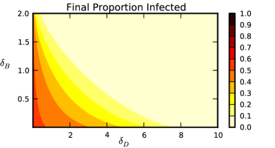
Figure 5: Final sizes of epidemics with behavior change. We use networks of the same structure as in Fig. 3. The disease spreads with $\beta=2$,  $\gamma=1$. The values of $\delta_{B}$ and $\delta_{D}$ are varied. For the initial condition, no individuals have changed behavior and a proportion $10^{-6}$ is initially infected randomly.

Summary

We have introduced an analytic model that calculates the simultaneous spread of two infectious diseases in a configuration model network. Our model is low-dimensional regardless of the degree distribution. Using this model, we are able to calculate the effect of interactions between diseases in regimes that are inaccessible to analytic theories that do not include dynamics.

This model can easily be generalized to a range of other “infectious” processes. We have shown its application to behavior changes in response to a disease.

Appendix A Appendix

Detailed derivation of equations

We begin with a configuration model network, and consider two infectious diseases which infect nodes of the network. We assume infection by either disease confers immediate and complete protection from any future infection by any disease. We index the diseases by $1$ and $2$. Individuals infected by disease $i=1,2$ transmit to their partners at rate $\beta_{i}$, and recover at rate $\gamma_{i}$.

We assume that at the initial time $t_{0}$ enough individuals are infected that the disease spreads deterministically (at the aggregated population-level), and that the probability an individual of degree $k$ is initially infected is $S(k,t_{0})$. We must make an assumption about which individuals are initially infected. Namely, if we consider an initially susceptible individual $u$, no information we have about $u$ at time $t_{0}$ tells us anything about the status of its partners. This assumption is satisfied if we initially infect a random subset of the population, or even if the disease has been spreading for some time before $t_{0}$. This assumption is violated if we select high-degree individuals and preferentially infect their partners.

The test individual

We now introduce the concept of a test individual. This concept is described in more detail in miller:final , and it allows us to simplify our calculations.

Whether a given individual $u$ is infected at any given time is a random variable. However, if we make the assumption that the disease spreads deterministically at the aggregated population-level, then whether or not a given individual is infected at any given time cannot have any impact on the aggregated scale. If it did, there would be stochastic effects visible at the population scale.

This observation allows us to decouple the status of $u$ from the dynamics of the epidemic in the sense that we can ignore any feedback from $u$ on the epidemic. To make this mathematically rigorous, we simply allow $u$ to become infected and for its infection to proceed as normal, but we disallow any transmission from $u$ to its partners. This keeps the status of partners of $u$ independent.

The probability that $u$ is susceptible equals the probability that none of its partners has transmitted to it (under the assumption $u$ does not transmit to its partners). To calculate the proportion of the population that is susceptible, infected, or recovered, we assume that $u$ is randomly selected from the population and prevented from infecting its partners. We call $u$ a test individual. The probability $u$ has a given status equals the proportion of the population that has that status.

Deriving the flow diagrams

We define $\theta(t)$ to be the probability that a random neighbor of $u$ which had not transmitted to $u$ by time $t=t_{0}$ still has not transmitted by time $t$. Then if $u$ has degree $k$, the probability it was initially susceptible is $S(k,t_{0})$, and the probability it is still susceptible is $S(k,t_{0})\theta(t)^{k}$. Averaging over all possible values of $k$, we have

$$S(t)=\psi(\theta(t))=\sum_{k}P(k)S(k,t_{0})\theta(t)^{k}$$

The value of $S$ reduces over time as infections occur. Mathematically this appears as a reduction in $\theta$. We must calculate how quickly $\theta$ changes, and how much of that change is due to each disease. This will allow us to calculate how much of the reduction in $S$ should go into each disease’s infected class.

We now look for the change in $\theta$. We define $v$ to be a random neighbor of $u$ which had not transmitted to $u$ by $t_{0}$. Then $\theta$ is the probability $v$ has not transmitted to $u$ by time $t$. As our initial condition, we have $\theta(t_{0})=1$. We divide $\theta$ into four compartments. We take $\phi_{S}$ to be the probability that $v$ is still susceptible, $\phi_{I,1}$ the probability $v$ is infected with disease $1$ but has not transmitted to $u$, $\phi_{I,2}$ the probability $v$ is infected with disease $2$ but has not transmitted to $u$, and $\phi_{R}$ the probability that $v$ is recovered (from either disease) and did not transmit during infection. These add up to $\theta$: $\theta=\phi_{S}+\phi_{I,1}+\phi_{I,2}+\phi_{R}$. The probability that $v$ has transmitted to $u$ is $1-\theta$. The flow between these compartments is shown in figure 6.

Figure 6: Flow diagram that leads to the evolution of $\theta$. A label along an edge gives the flux of probability along that edge.

We first find the rate of change of $\theta$. It is relatively straightforward to see that

$$\dot{\theta}=-\beta_{1}\phi_{I,1}-\beta_{2}\phi_{I,2}$$

This is because the only path for $\theta$ to decrease is through $v$ transmitting to $u$, which requires that $v$ be infected (and not yet transmitted to $u$).

At $t_{0}$, we have $\phi_{S}(t_{0})$ is the probability a random neighbor of $u$ is still susceptible (given that it has not transmitted to $u$). We take this as an input value. The value of $\phi_{I,1}$, $\phi_{I,2}$, and $\phi_{R}$ are similarly all input from the conditions at $t_{0}$. We can explicitly calculate the value of $\phi_{S}$ at later times, if we know $\theta$. To do this, we find the probability distribution for degree of $v$, and then calculate the probability that no neighbor of $v$ has transmitted to $v$.

At time $t_{0}$, the edge joining $u$ to $v$ is simply an edge from $u$ to a random neighbor that is susceptible. The probability that edge connects to a degree $k$ individual is proportional to the number of edges that all susceptible individuals of degree $k$ have, $NkP(k)S(k,t_{0})$. The normalization factor is the total number of all edges of susceptible individuals, $\sum_{k^{\prime}}Nk^{\prime}P(k^{\prime})S(k^{\prime},t_{0})$. The probability that $v$ is still susceptible at time $t$ is $\theta(t)^{k-1}$. So the probability of having a degree $k$ susceptible neighbor at time $t$ is $NkP(k)S(k,t_{0})\theta(t)^{k-1}/\sum_{k^{\prime}}Nk^{\prime}P(k^{\prime})S(k^{\prime},t_{0})$. Summing over all possible $k$, and cancelling $N$, we arrive at $\sum_{k}kP(k)S(k,t_{0})\theta(t)^{k-1}/\sum_{k^{\prime}}k^{\prime}P(k^{\prime})S(k^{\prime},t_{0})=\psi^{\prime}(\theta(t))/\psi^{\prime}(1)$. So given that $v$ is initially susceptible, the probability that $v$ is susceptible at a later time $t$ is $\psi^{\prime}(\theta(t))/\psi^{\prime}(1)$. Since the probability $v$ is initially susceptible is $\phi_{S}(t_{0})$, we conclude

$$\phi_{S}(t)=\phi_{S}(t_{0})\frac{\psi^{\prime}(\theta)}{\psi^{\prime}(1)}$$

The rate of change of $\phi_{S}$ is simply $\phi_{S}(t_{0})\dot{\theta}\psi^{\prime\prime}(\theta)/\psi^{\prime}(1)$. It is straightforward to see that the amount that goes from $\phi_{S}$ to $\phi_{I,1}$ is $\phi_{S}(t_{0})\beta_{1}\phi_{I,1}\psi^{\prime\prime}(\theta)/\psi^{\prime}(1)$ and the amount going into $\phi_{I,2}$ is $\beta_{2}\phi_{I,2}\psi^{\prime\prime}(\theta)/\psi^{\prime}(1)$.

So in figure 6, we have expressions for the flux along each edge except the edges into $\phi_{R}$. These edges are straightforward, because the recovery rate for disease $1$ is $\gamma_{1}$ and the recovery rate for disease $2$ is $\gamma_{2}$. So the total flux from $\phi_{I,1}$ to $\phi_{R}$ is $\gamma_{1}\phi_{I,1}$ and the flux from $\phi_{I,2}$ is $\gamma_{2}\phi_{I,2}$.

Using the flows in figure 6, we can arrive at a coupled system for $\theta$, $\phi_{I,1}$ and $\phi_{I,2}$. It is

$$\dot{\theta} =-\beta_{1}\phi_{I,1}-\beta_{2}\phi_{I,2}$$

$$\dot{\phi}_{I,1} =-(\beta_{1}+\gamma_{1})\phi_{I,1}+\beta_{1}\phi_{I,1}\phi_{S}(t_{0})\frac{\psi^{\prime\prime}(\theta)}{\psi^{\prime}(1)}$$

$$\dot{\phi}_{I,2} =-(\beta_{2}+\gamma_{2})\phi_{I,2}+\beta_{2}\phi_{I,2}\phi_{S}(t_{0})\frac{\psi^{\prime\prime}(\theta)}{\psi^{\prime}(1)}$$

with $\theta(t_{0})=1$ and $\phi_{S}(t_{0})$, $\phi_{I,1}(t_{0})$, and $\phi_{I,2}(t_{0})$ given by the initial state of the population.

These equations govern the spread of the disease through the network. However, they are not the usual variables of interest. Typically we want to know the proportion susceptible, infected, or recovered. Figure 7 shows a flow diagram governing the proportion of the population in each state. We can use this to recover $S$, $I_{1}$, $I_{2}$, $R_{1}$, and $R_{2}$. As we noted above, $S(t)=\psi(\theta)$. The flux into $I_{1}$ can be calculated to be $\beta_{1}\phi_{I,1}\psi^{\prime}(\theta)$, and the flux into $I_{2}$ is $\beta_{2}\phi_{I,2}\psi^{\prime}(\theta)$. The fluxes from each of these into the recovered states are $\gamma_{1}I_{1}$ and $\gamma_{2}I_{2}$. We distinguish the two recovered states because we will frequently be interested in the total proportion infected by each disease. We could have similarly subdivided $\phi_{R}$ into two compartments, but it would not provide any information that is useful here.

Figure 7: Flow diagram leading to equations for the proportion of the population in each compartment.

Thus our final system of equations is

$$\dot{\theta} =-\beta_{1}\phi_{I,1}-\beta_{2}\phi_{I,2}$$

$$\dot{\phi}_{I,1} =-(\beta_{1}+\gamma_{1})\phi_{I,1}+\beta_{1}\phi_{I,1}\phi_{S}(t_{0})\frac{\psi^{\prime\prime}(\theta)}{\psi^{\prime}(1)}$$

$$\dot{\phi}_{I,2} =-(\beta_{2}+\gamma_{2})\phi_{I,2}+\beta_{2}\phi_{I,2}\phi_{S}(t_{0})\frac{\psi^{\prime\prime}(\theta)}{\psi^{\prime}(1)}$$

$$S =\psi(\theta)$$

$$\dot{I}_{1} =\beta_{1}\phi_{I,1}\psi^{\prime}(\theta)-\gamma_{1}I_{1}$$

$$\dot{I}_{2} =\beta_{2}\phi_{I,2}\psi^{\prime}(\theta)-\gamma_{2}I_{2}$$

$$\dot{R}_{1} =\gamma_{1}I_{1}$$

$$\dot{R}_{2} =\gamma_{2}I_{2}$$

Regime Analysis

There are several regimes that can be identified. When the cumulative number of infections is small enough that $S$ and $\phi_{S}$ are approximately $1$, then we can neglect nonlinear terms. Which regime is observed is determined by the relative sizes of the two epidemics when the linear approximation breaks down. We focus our attention on regimes for which the linear approximation is valid at the initial time.

When the initial condition is small, the linear terms dominate and the epidemics grow (or decay) exponentially. The equations governing the epidemics are uncoupled in this regime. Physically, this means that competition for nodes is so weak that it can be neglected. In fact a stronger statement is true: in addition to not having inter-disease competition, there is no intra-disease competition: a transmission path is very unlikely to encounter a node infected along another transmission path.

Assume that the exponential growth rates of the two diseases are $r_{1}$ and $r_{2}$, with $r_{1}\geq r_{2}$. This continues until one of them becomes large enough that competition begins to appear. At this point the growth of both epidemics starts to slow. If the difference in epidemic sizes is large enough at this point, then this first epidemic will not be slowed by the much smaller other epidemic. The dynamics will proceed as if there were just one disease spreading. Eventually the susceptible population will decrease, the disease will peak and eventually decay away, all with the second disease negligible. Once this decay has occurred, there will be a “residual” network. The second disease will continue to spread along this network. If the residual network is well-enough connected (and the second disease sufficiently infectious), the second disease can continue to grow, and then it experiences its own epidemic.

If the diseases are close enough in size when nonlinear terms become important, then both diseases contribute a non-negligible amount to reduction in $S$ and $\phi_{S}$ at the same time. Thus they interact dynamically. Each disease contributes in a non-negligible way to hindering the spread of the other. To determine whether this can happen, we use a simple balance based on the initial sizes and the early growth rates. Typically we might expect that one disease becomes large while the other is still exponentially small.

If one disease is sufficiently small when the other disease becomes large, then the larger disease will spread and cause an epidemic that is effectively the same size as it would be in the absence of the smaller disease. Using the initial sizes and growth rates, it is straightforward to calculate the sizes of the two diseases once nonlinearities begin to be significant. For the two diseases to not interact, the “smaller” disease must remain negligibly small until the “larger” disease has finished its epidemic. We derive slightly different thresholds for the case where the smaller disease is the fast-growing disease or the slow-growing disease. To derive the threshold condition, we make a crude assumption that the two diseases continue spreading according to the linear growth rate. In the non-overlapping regimes, the smaller disease must remain small throughout the spread of the larger disease. We crudely choose to apply our conditions when the exponential growth implies that the larger disease would have reached size $1$. We look at the size of the smaller disease (assuming exponential growth) at this time. For a given observed size for the smaller disease, we reach different conclusions if it is the fast or the slow growing disease. If it is the fast-growing disease, and we observe $0.05$, then that means that at previous times it was much smaller, and so we would not expect to observe any impact. On the other hand if it is the slower-growing disease, and we observe $0.05$, that means for much of the spread of the larger disease it was at about that size, and so we would expect to observe some impact. So if the fast-growing disease is the small disease, we allow it to be as large as $0.05$ when the slow disease would reach $1$. If the slow-growing disease is the small disease, we require that it be much smaller, choosing $0.0025=0.05^{2}$ instead. Our choice of threshold is somewhat arbitrary, and influenced by the fact that $\ln 0.05\approx-3$ giving a simple expression for our thresholds. Taking this, we can derive the $C_{\text{min}}\approx-6$ and $C_{\text{max}}\approx 3r_{2}/r_{1}$ thresholds in the text.

Taking $\rho_{1}$ and $\rho_{2}$ to be the proportions initially infected with each disease (at random). So long as $C=\ln\rho_{2}-(r_{2}/r_{1})\ln\rho_{1}$ is not between $-6$ and $3r2/r1$, then the two diseases will not interact dynamically. One disease will become large and run through its entire epidemic prior to the other disease (possibly) having its own epidemic. This defines the “non-overlapping” epidemic regimes. If $C$ lies within this range, then we have the overlapping epidemic regime.

Impact of Behavior change

Figure 8: The flow diagrams underlying the spread of an infectious disease in the presence of a behavior change. We assume behavior change can be triggered by contact with an infected individual or with an individual who has already adopted the change. We assume behavior change provides complete immunity to disease.

We now consider the spread of a single disese through a network, which can be prevented with a behavior change. We assume that the behavior change gives complete protection from infection. Once an individual has adopted the behavior change, the change is permanent. An individual who has changed behavior will transmit that behavior change to partners.

The disease transmits at rate $\beta$ and recovery occurs at rate $\gamma$. Contact with an infected individual causes behavior change at rate $\delta_{D}$. Contact with an individual whose behavior has changed causes behavior change at rate $\delta_{B}$. The flow diagrams are shown in figure 8. The resulting equations are

$$\dot{\theta} =-(\beta_{D}+\delta_{D})\phi_{D}-\delta_{B}\phi_{B}$$

$$\dot{\phi}_{B} =(\delta_{B}\phi_{B}+\delta_{D}\phi_{D})\phi_{S}(t_{0})\frac{\psi^{\prime\prime}(\theta)}{\psi^{\prime}(1)}$$

$$\dot{\phi}_{D} =\beta_{D}\phi_{D}\phi_{S}(t_{0})\frac{\psi^{\prime\prime}(\theta)}{\psi^{\prime}(1)}-(\beta_{D}+\delta_{D}+\gamma)\phi_{D}$$

$$\dot{I} =\beta_{D}\phi_{D}\psi^{\prime}(\theta)-\gamma I$$

$$\dot{B} =(\delta_{B}\phi_{B}+\delta_{D}\phi_{D})\psi^{\prime}(\theta)$$

$$\dot{R} =\gamma I$$

$$S =\psi(\theta)$$

The early growth of $\phi_{D}$ is exponential with rate $\beta_{D}\phi_{S}(t_{0})\psi^{\prime\prime}(1)/\psi^{\prime}(1)-(\beta_{D}+\delta_{D}+\gamma)$. If $\delta_{D}$ is sufficiently large, the infection decays. This corresponds to a balance between transmitting disease prior to either recovering or transmitting behavior change. When the transmission probability is small enough a typical infected individual causes fewer than $1$ new infection and the disease must die out.

Changing $\delta_{B}$ does not alter the early growth rate of the disease. So we might anticipate that the disease will be able to cause a large scale epidemic. However, if $\delta_{B}>0$, the behavior change itself also leads to an “epidemic”. If the behavior growth rate is sufficiently large, its “epidemic” occurs while the disease epidemic is still exponentially small. In this limit, the behavior change will dominate the populaion, and the disease remains exponentially small. We do not see the complementary case in which the disease becomes large while the behavior change is exponentially small, because as disease incidence increases it directly induces behavior changes. So either the behavior change has its “epidemic” first, or the two have overlapping “epidemics”.

References

- [1] Viggo Andreasen, J. Lin, and S.A. Levin. The dynamics of cocirculating influenza strains conferring partial cross-immunity. Journal of mathematical biology, 35(7):825–842, 1997.
- [2] S. Bharathi, D. Kempe, and M. Salek. Competitive influence maximization in social networks. Internet and Network Economics, pages 306–311, 2007.
- [3] Marián Boguñá, Romualdo Pastor-Satorras, and Alessandro Vespignani. Absence of epidemic threshold in scale-free networks with degree correlations. Physical Review Letters, 90(2):028701, 2003.
- [4] S. Cobey and M. Pascual. Consequences of host heterogeneity, epitope immunodominance, and immune breadth for strain competition. Journal of Theoretical Biology, 270(1):80–87, 2011.
- [5] Laurent Decreusefond, Jean-Stéphane Dhersin, Pascal Moyal, and Viet Chi Tran. Large graph limit for an SIR process in random network with heterogeneous connectivity. The Annals of Applied Probability, 22(2):541–575, 2012.
- [6] R. Durrett, J.P. Gleeson, A.L. Lloyd, P.J. Mucha, F. Shi, D. Sivakoff, J.E.S. Socolar, and C. Varghese. Graph fission in an evolving voter model. Proceedings of the National Academy of Sciences, 109(10):3682–3687, 2012.
- [7] K. T. D. Eames. Modelling disease spread through random and regular contacts in clustered populations. Theoretical Population Biology, 73:104–111, 2008.
- [8] K.T.D. Eames and M.J. Keeling. Modeling dynamic and network heterogeneities in the spread of sexually transmitted diseases. Proceedings of the National Academy of Sciences, 99(20):13330–13335, 2002.
- [9] S. Funk, E. Gilad, C. Watkins, and V.A.A. Jansen. The spread of awareness and its impact on epidemic outbreaks. Proceedings of the National Academy of Sciences, 106(16):6872, 2009.
- [10] S. Funk and V.A.A. Jansen. Interacting epidemics on overlay networks. Physical Review E, 81:036118, 2010.
- [11] J.P. Gleeson, S. Melnik, and A. Hackett. How clustering affects the bond percolation threshold in complex networks. Physical Review E, 81(6):066114, 2010.
- [12] T. House and M.J. Keeling. Insights from unifying modern approximations to infections on networks. Journal of The Royal Society Interface, 2010.
- [13] B. Karrer and MEJ Newman. Competing epidemics on complex networks. Physical Review E, 84(3):036106, 2011.
- [14] Brian Karrer and Mark E. J. Newman. Message passing approach for general epidemic models. Physical Review E, 82:016101, 2010.
- [15] Eben Kenah and James M. Robins. Second look at the spread of epidemics on networks. Physical Review E, 76(3):036113, 2007.
- [16] D.B. Larremore, W.L. Shew, and J.G. Restrepo. Predicting criticality and dynamic range in complex networks: effects of topology. Physical review letters, 106(5):58101, 2011.
- [17] Robert M. May and Alun L. Lloyd. Infection dynamics on scale-free networks. Physical Review E, 64(6):066112, Nov 2001.
- [18] S. Melnik, A. Hackett, M.A. Porter, P.J. Mucha, and J.P. Gleeson. The unreasonable effectiveness of tree-based theory for networks with clustering. Physical Review E, 83(3):036112, 2011.
- [19] Joel C. Miller. Epidemic size and probability in populations with heterogeneous infectivity and susceptibility. Physical Review E, 76(1):010101(R), 2007.
- [20] Joel C. Miller. Bounding the size and probability of epidemics on networks. Journal of Applied Probability, 45:498–512, 2008.
- [21] Joel C. Miller. Percolation and epidemics in random clustered networks. Physical Review E, 80(2):020901(R), 2009.
- [22] Joel C. Miller. Spread of infectious disease through clustered populations. Journal of The Royal Society Interface, 6(41):1121, 2009.
- [23] Joel C. Miller. A note on the derivation of epidemic final sizes. Bulletin of Mathematical Biology, 74(9):2125–2141, 2012.
- [24] Joel C. Miller, Anja C. Slim, and Erik M. Volz. Edge-based compartmental modelling for infectious disease spread. Journal of the Royal Society Interface, 9(70):890–906, 2012.
- [25] Joel C. Miller and Erik M. Volz. Edge-based compartmental modeling with disease and population structure. submitted Available at http://arxiv.org/abs/1106.6344.
- [26] Joel C. Miller and Erik M. Volz. Model hierarchies in edge-based compartmental modeling for infectious disease spread. Journal of Mathematical Biology, 2012.
- [27] M. Molloy and Bruce Reed. A critical point for random graphs with a given degree sequence. Random Structures & Algorithms, 6(2):161–179, 1995.
- [28] Mark E. J. Newman. Spread of epidemic disease on networks. Physical Review E, 66(1):016128, 2002.
- [29] Mark E. J. Newman. The structure and function of complex networks. SIAM Review, 45:167–256, 2003.
- [30] Mark E. J. Newman. Threshold effects for two pathogens spreading on a network. Physical Review Letters, 95(10):108701, 2005.
- [31] Mark E. J. Newman. Random graphs with clustering. Physical Review Letters, 103(5):58701, 2009.
- [32] Romualdo Pastor-Satorras and Alessandro Vespignani. Epidemic dynamics and endemic states in complex networks. Physical Review E, 63(6):066117, 2001.
- [33] Romualdo Pastor-Satorras and Alessandro Vespignani. Epidemic spreading in scale-free networks. Physical Review Letters, 86(14):3200–3203, Apr 2001.
- [34] Pieter Trapman. On analytical approaches to epidemics on networks. Theoretical Population Biology, 71(2):160–173, 2007.
- [35] Erik M. Volz and Lauren Ancel Meyers. Susceptible–infected–recovered epidemics in dynamic contact networks. Proceedings of the Royal Society B: Biological Sciences, 274(1628):2925–2933, 2007.
- [36] Erik M. Volz, Joel C. Miller, Alison Galvani, and Lauren Ancel Meyers. Effects of heterogeneous and clustered contact patterns on infectious disease dynamics. PLoS Comput Biol, 7(6):e1002042, 06 2011.