Fluctuations in the Time Variable and Dynamical Heterogeneity in Glass-Forming Systems

Abstract

We test a hypothesis for the origin of dynamical heterogeneity in slowly relaxing systems, namely that it emerges from soft (Goldstone) modes associated with a broken continuous symmetry under time reparametrizations. We do this by constructing coarse grained observables and decomposing the fluctuations of these observables into transverse components, which are associated with the postulated time-fluctuation soft modes, and a longitudinal component, which represents the rest of the fluctuations. Our test is performed on data obtained in simulations of four models of structural glasses. As the hypothesis predicts, we find that the time reparametrization fluctuations become increasingly dominant as temperature is lowered and timescales are increased. More specifically, the ratio between the strengths of the transverse fluctuations and the longitudinal fluctuations grows as a function of the dynamical susceptibility, $\chi_{4}$, which represents the strength of the dynamical heterogeneity; and the correlation volumes for the transverse fluctuations are approximately proportional to those for the dynamical heterogeneity, while the correlation volumes for the longitudinal fluctuations remain small and approximately constant.

I Introduction

The rapidly increasing relaxation timescales, the presence of non-exponential relaxation, as well as the violation of Stokes-Einstein relations between viscosity and diffusivity are some features observed close to the glass transition in glassy systems Debenedetti2001 ; Ediger2000 ; Sillescu . The appearance of these features suggests that relaxation dynamics is heterogeneous, i.e. that it is faster in some regions and slower in others Ediger2000 ; Sillescu ; Berthier2011 . Direct microscopic evidence for this behavior has been found both in simulations Berthier2011 ; Lacevic and in experiments Berthier2011 ; VidalRussell1998 ; Walther1998 ; Russell2000 ; Kegel2000 ; Weeks2000 ; Weeks2002 ; Courtland2003 ; Cipelleti ; Keys2007 ; Abate2007 ; Duri2009 . The understanding of dynamical heterogeneity is believed to be crucial to explain anomalous behavior of materials near the glass transition, and even possibly to explain the very presence of the glass transition itself Ediger2000 . Despite many efforts trying to address the origin of dynamical heterogeneity, this question still remains open Berthier2011 ; Toninelli ; Garrahan ; Lubchenko ; Castillo2003 .

In recent years, different tools have been used to probe dynamical heterogeneity. One such tool is the dynamical susceptibility, $\chi_{4}$, which depends both on the strength of the local fluctuations and the spatial extent of their correlations. The peak value of $\chi_{4}$ has been observed to grow while approaching the glass transition. However, this tool by itself cannot tell us much about the origin of dynamical heterogeneity and it may be desirable to supplement it with other ways of probing the fluctuations in the system.

In this work, we test the predictions of a theoretical framework that aims to describe the slow part of the fluctuations in the relaxation dynamics Castillo2003 ; Chamon2002 ; Castillo2002 ; Chamon2004 ; Chamon2007 . This framework is based on the hypothesis that in glassy systems the long time dynamics is invariant under reparametrizations of the time variable Castillo2003 ; Chamon2002 ; Castillo2002 ; Chamon2004 ; Chamon2007 ; Castillo2008 ; Mavimbela2011 ; Franz2010 ; Franz2011 , but this invariance is broken, giving rise to Goldstone modes that manifest themselves with the emerge of heterogeneous dynamics Castillo2003 ; Chamon2002 ; Castillo2002 ; Chamon2004 ; Chamon2007 ; Castillo2007 ; Parsaeian2008 ; Parsaeian2009 ; Parsaeian2008a ; Avila ; Mavimbela . The Goldstone modes correspond to fluctuations in the time reparametrization $t\rightarrow\phi_{\vec{r}}(t)$, i.e.

$$C_{\vec{r}}(t,t^{\prime})\approx C[\phi_{\vec{r}}(t),\phi_{\vec{r}}(t^{\prime})],$$ (1)

where $C(t,t^{\prime})$ is a global two–time correlation function. Some indirect evidence in favor of the presence of this kind of fluctuation in structural glasses has been presented in Castillo2007 ; Parsaeian2008 ; Parsaeian2009 ; Parsaeian2008a . In this work, we present results for a more direct test, based on decomposing fluctuations into a transverse part satisfying Eq. (1) and a longitudinal part containing all other fluctuations. This procedure allows one to separately quantify the strength and spatial correlations of both kinds of fluctuations, as a function of temperature and timescales, for a variety of glass-forming models both below and above the mode coupling critical temperature $T_{c}$. The same kind of test can also be applied to particle tracking experimental data from colloidal and granular systems Berthier2011 ; Kegel2000 ; Weeks2000 ; Weeks2002 ; Courtland2003 ; Cipelleti ; Keys2007 ; Abate2007 , thus allowing to investigate a possible unified explanation of dynamical heterogeneity in diverse systems. A summary of the results of an early version of our analysis was published in Ref. Avila .

This manuscript is organized in the following way. In Sec. II we discuss the hypothesis and define the quantities we use to test it. In Sec. III we present the details of the numerical simulations used to test the hypothesis and present the results of our analysis. Finally, we discuss our conclusions in Sec. IV.

II Time reparametrization invariance and fluctuations

We start by discussing in general terms the expected effects of time reparametrization invariance on the fluctuations. Let us consider the global two–time correlation function

$$C(t,t^{\prime})=\left\langle\frac{1}{N}\sum_{j=1}^{N}\cos\{\vec{q}\cdot[\vec{r}_{j}(t)-\vec{r}_{j}(t^{\prime})]\}\right\rangle,$$ (2)

where $N$ is the number of particles, $\vec{r}_{j}(t)$ is the position of particle $j$ at time $t$, and $\vec{q}$ is the wave-vector that corresponds to the main peak of the static structure factor. Here $\langle\cdots\rangle$ denotes an average over thermal fluctuations, which in our case is approximated by an average over independent molecular dynamics (MD) runs. In equilibrium, and more generally in time translationally invariant (TTI) systems, this correlation function depends only on the difference between the two times $t-t^{\prime}$. In the case of aging, the system is no longer TTI and $C(t,t^{\prime})$ depends nontrivially on both times $t$ and $t^{\prime}$.

To analyze the fluctuations in the dynamics we define the local correlation as Castillo2007 ; Parsaeian2008 ; Parsaeian2009 ; Parsaeian2008a

$$C_{\vec{r}}(t,t^{\prime})=\frac{1}{N(B_{r})}\sum_{r_{j}(t^{\prime})\in B_{r}}\cos\{\vec{q}\cdot[\vec{r}_{j}(t)-\vec{r}_{j}(t^{\prime})]\},$$ (3)

where the average over particles in Eq. (2) is now restricted to a region $B_{\vec{r}}$ around point $\vec{r}$, which contains $N(B_{\vec{r}})$ particles at time $t^{\prime}<t$. $C_{\vec{r}}(t,t^{\prime})$ probes the mobility of the particles in a region near $\vec{r}$ between times $t^{\prime}$ and $t$: it is close to zero for regions where the particle configuration has changed significantly, and much closer to unity for regions where it has changed little or not at all.

In this work we will consider a slightly more restrictive version of Eq. (1), namely Avila ; Bouchaud ; Notation

$$C_{\vec{r}}(t,t^{\prime})\approx g[\phi_{\vec{r}}(t)-\phi_{\vec{r}}(t^{\prime})],$$ (4)

which corresponds to the case when the global correlation has the form Avila ; Bouchaud ; Notation

$$C(t,t^{\prime})=g[\phi(t)-\phi(t^{\prime})].$$ (5)

In principle, the functions $g(x)$ in Eqs. (4) and (5) could be different. For example, it has been claimed Ediger2000 that stretched-exponential global relaxation could be the result of combining local exponential relaxations with different relaxation times, in which case we would have $g_{\rm global}=A\exp{(-|x|^{\beta})}$ in Eq. (5) and $g_{\rm local}=A^{\prime}\exp{(-|x|)}$ in Eq. (4) Mavimbela . In this work, for simplicity, we impose the condition $g_{\rm global}(x)=g_{\rm local}(x)=g(x)$. Both this restriction and the restriction imposed in Eq. (5) could in principle make the results appear to be slightly less consistent with the hypothesis than they would be otherwise. The forms of the functions $g(x)$ and $\phi(t)$ can be obtained by fitting the global correlation $C(t,t^{\prime})$, as we do in the next section. We will assume, for the moment, that $g(x)$ and $\phi(t)$ are known.

As mentioned before, we refer to the fluctuations described by Eq. (4) as transverse fluctuations and the rest of the fluctuations as longitudinal fluctuations phi . To visualize these ideas in more detail, we define

$$\Phi_{ab,{\vec{r}}}\equiv g^{-1}(C_{ab,{\vec{r}}}),$$ (6)

with $a,b\in\{1,2,3\}$ Notation , where $C_{ab,{\vec{r}}}\equiv C_{\vec{r}}(t_{a},t_{b})$. The fluctuating quantity $\Phi_{ab,{\vec{r}}}$ is composed of a transverse contribution,

$$\Phi_{ab,{\vec{r}}}{}^{T}=\phi_{\vec{r}}(t_{a})-\phi_{\vec{r}}(t_{b}),$$ (7)

and a longitudinal contribution, $\Phi_{ab,{\vec{r}}}{}^{L}$, i.e.,

$$g^{-1}(C_{ab,{\vec{r}}})=\Phi_{ab,{\vec{r}}}=\Phi_{ab,{\vec{r}}}{}^{T}+\Phi_{ab,{\vec{r}}}{}^{L}=\phi_{\vec{r}}(t_{a})-\phi_{\vec{r}}(t_{b})+\Phi_{ab,{\vec{r}}}{}^{L}.$$ (8)

This means that in the absence of longitudinal fluctuations, Eq. (4) would be exact. In order to quantify both kinds of fluctuations, we define

$${\sigma_{\vec{r}}} \equiv \frac{1}{\sqrt{3}}\left[g^{-1}(C_{21,{\vec{r}}})+g^{-1}(C_{32,{\vec{r}}})-g^{-1}(C_{31,{\vec{r}}})\right]$$ (9)

$$=\frac{1}{\sqrt{3}}\left(\Phi_{21,{\vec{r}}}{}^{L}+\Phi_{32,{\vec{r}}}{}^{L}-\Phi_{31,{\vec{r}}}{}^{L}\right),$$

$${\pi}_{1,{\vec{r}}} \equiv \frac{1}{\sqrt{2}}\left[g^{-1}(C_{21,{\vec{r}}})-g^{-1}(C_{32,{\vec{r}}})\right]$$ (10)

$$= \frac{1}{\sqrt{2}}\left[(\Phi_{21,{\vec{r}}}{}^{T}+\Phi_{21,{\vec{r}}}{}^{L})-(\Phi_{32,{\vec{r}}}{}^{T}+\Phi_{32,{\vec{r}}}{}^{L})\right],$$

and

$${\pi}_{2,{\vec{r}}} \equiv \frac{1}{\sqrt{6}}\left[g^{-1}(C_{21,{\vec{r}}})+g^{-1}(C_{32,{\vec{r}}})+2g^{-1}(C_{31,{\vec{r}}})\right]$$ (11)

$$= \frac{1}{\sqrt{6}}\left[(\Phi_{21,{\vec{r}}}{}^{T}+\Phi_{21,{\vec{r}}}{}^{L})+(\Phi_{32,{\vec{r}}}{}^{T}+\Phi_{32,{\vec{r}}}{}^{L})+2(\Phi_{31,{\vec{r}}}{}^{T}+\Phi_{31,{\vec{r}}}{}^{L})\right],$$

with $t_{1}<t_{2}<t_{3}$. As shown above, ${\sigma_{\vec{r}}}$ contains only longitudinal fluctuations, but $\pi_{1,{\vec{r}}}$ and $\pi_{2,{\vec{r}}}$ contain both transverse and longitudinal components. If Eq. (4) was an exact identity, the local two-time function would verify the following relation:

$$g^{-1}(C_{21,{\vec{r}}})+g^{-1}(C_{32,{\vec{r}}})-g^{-1}(C_{31,{\vec{r}}})=0.$$ (12)

Then, in the case where no longitudinal fluctuations are present, the vector $(\sigma_{\vec{r}},\pi_{1,{\vec{r}}},\pi_{2,{\vec{r}}})$ would be restricted to be fluctuating in the plane $\sigma_{\vec{r}}=0$. We expect that as the temperature becomes lower, the timescales become longer, and the system becomes more glassy, transverse fluctuations should become progressively more dominant, according to the hypothesis [Eq. (1)] and therefore the probability distribution $\rho(\sigma_{\vec{r}},\pi_{1,{\vec{r}}},\pi_{2,{\vec{r}}})$ should become anisotropic, extending mostly along the $\sigma_{\vec{r}}=0$ plane and not away from it.

An analogous set of quantities can be defined starting from the global correlation $C(t,t^{\prime})$. We can write the analogs of Eqs. (7) and (8), i.e.

$$\Phi_{ab}{}^{T}=\phi(t_{a})-\phi(t_{b}),$$ (13)

$$g^{-1}[C(t_{a},t_{b})]=\Phi_{ab}=\Phi_{ab}{}^{T}+\Phi_{ab}{}^{L}=\phi(t_{a})-\phi(t_{b})+\Phi_{ab}{}^{L}.$$ (14)

However, in this case, the meanings of the symbols are different. $\Phi_{ab}{}^{T}$ and $\Phi_{ab}{}^{L}$ do not fluctuate, because they are computed from the global correlation in the thermodynamic limit, which is self averaging. If Eq. (5) was exact, then $\Phi_{ab}{}^{L}\equiv 0$. However, in practice Eq. (5) is only approximate: in Sec. III we fit the left-hand side by an expression with the form given in the right-hand side. Thus $\Phi_{ab}{}^{T}$ represents the part of $\Phi_{ab}$ that can be represented as a difference $\phi(t_{a})-\phi(t_{b})$ according to the fits, and $\Phi_{ab}{}^{L}$ represents the part of $\Phi_{ab}$ that the fit does not capture, or in other words a fitting error. Additionally, the global variables $\sigma$, $\pi_{1}$ and $\pi_{2}$ can be defined, by analogy to Eqs. (9), (10), and (11), in the following way:

$${\sigma}\equiv\frac{1}{\sqrt{3}}\left(\Phi_{21}+\Phi_{32}-\Phi_{31}\right)=\frac{1}{\sqrt{3}}\left(\Phi_{21}{}^{L}+\Phi_{32}{}^{L}-\Phi_{31}{}^{L}\right),$$ (15)

$${\pi}_{1}\equiv\frac{1}{\sqrt{2}}\left(\Phi_{21}-\Phi_{32}\right),$$ (16)

and

$${\pi}_{2}\equiv\frac{1}{\sqrt{6}}\left(\Phi_{21}+\Phi_{32}+2\Phi_{31}\right),$$ (17)

with $t_{1}<t_{2}<t_{3}$. If Eq. (5) was an exact identity, i.e., if the fit of $C(t,t^{\prime})$ by $g[\phi(t)-\phi(t^{\prime})]$ had exactly zero residuals, then $\sigma=0$ and the global two-time function would verify the relation

$$g^{-1}[C(t_{2},t_{1})]+g^{-1}[C(t_{3},t_{2})]-g^{-1}[C(t_{3},t_{1})]=0.$$ (18)

A more extensive analysis of the fluctuations can be performed by separating longitudinal and transverse components in Eqs. (10) and (11). First, we recall that $\sigma$ is a purely longitudinal quantity [see Eq. (9)], therefore $\sigma_{{\vec{r}}}{}^{T}=0$ and $\Phi_{31,{\vec{r}}}{}^{T}=\Phi_{21,{\vec{r}}}{}^{T}+\Phi_{32,{\vec{r}}}{}^{T}$. Now, we make the following two assumptions. One is that the transverse and longitudinal fluctuations are not correlated to each other. The other is that all slow fluctuations are transverse, or in other words, that longitudinal fluctuations are short range correlated in time, or at least they are correlated over times that are shorter than the shortest time interval between the configurations that are being considered. This leads to the conditions

$$\left\langle\delta\Phi_{ab,{\vec{r}}}{}^{L}\delta\Phi_{cd,{\vec{r}}^{\prime}}{}^{T}\right\rangle=0\quad\quad\forall\quad a,b,c,d,{\vec{r}},{\vec{r}}^{\prime}$$ (19)

and

$$\left\langle\delta\Phi_{ab,{\vec{r}}}{}^{L}\delta\Phi_{cd,{\vec{r}}^{\prime}}{}^{L}\right\rangle=0\quad\quad\text{for}\quad a\not=c\quad\text{or}\quad b\not=d,\quad\quad\forall\quad{\vec{r}},{\vec{r}}^{\prime}.$$ (20)

Here $\delta x\equiv x-\langle x\rangle$. By using Eq. (7), it can be shown that the transverse components of Eqs. (10) and (11) are given by

$$\pi_{1,{\vec{r}}}{}^{T}=\frac{1}{\sqrt{2}}(\Phi_{21,{\vec{r}}}{}^{T}-\Phi_{32,{\vec{r}}}{}^{T})$$ (21)

and

$$\pi_{2,{\vec{r}}}{}^{T}=\frac{3}{\sqrt{6}}(\Phi_{21,{\vec{r}}}{}^{T}+\Phi_{32,{\vec{r}}}{}^{T}).$$ (22)

Regarding the longitudinal components, by using Eq. (20) it can be shown that

$$\left\langle(\delta\sigma_{\vec{r}}{}^{L})^{2}\right\rangle=\frac{1}{3}\left[\left\langle(\delta\Phi_{21,{\vec{r}}}{}^{L})^{2}\right\rangle+\left\langle(\delta\Phi_{32,{\vec{r}}}{}^{L})^{2}\right\rangle+\left\langle(\delta\Phi_{31,{\vec{r}}}{}^{L})^{2}\right\rangle\right],$$ (23)

$$\left\langle(\delta\pi_{1,{\vec{r}}}{}^{L})^{2}\right\rangle=\frac{1}{2}\left[\left\langle(\delta\Phi_{21,{\vec{r}}}{}^{L})^{2}\right\rangle+\left\langle(\delta\Phi_{32,{\vec{r}}}{}^{L})^{2}\right\rangle\right],$$ (24)

and

$$\left\langle(\delta\pi_{2,{\vec{r}}}{}^{L})^{2}\right\rangle=\frac{1}{6}\left[\left\langle(\delta\Phi_{21,{\vec{r}}}{}^{L})^{2}\right\rangle+\left\langle(\delta\Phi_{32,{\vec{r}}}{}^{L})^{2}\right\rangle+4\left\langle(\delta\Phi_{31,{\vec{r}}}{}^{L})^{2}\right\rangle\right].$$ (25)

From the last three equations it can be easily seen that

$$\left\langle(\delta\pi_{1,{\vec{r}}}{}^{L})^{2}+(\delta\pi_{2,{\vec{r}}}{}^{L})^{2}-2(\delta\sigma_{\vec{r}}{}^{L})^{2}\right\rangle=0.$$ (26)

By using Eq. (19) we find that, all together, we can compute the variance of the transverse fluctuations by combining the fluctuations of Eqs. (9), (10), and (11) in the following way

$$\left\langle(\delta\pi_{1,{\vec{r}}}{}^{T})^{2}+(\delta\pi_{2,{\vec{r}}}{}^{T})^{2}\right\rangle=\left\langle(\delta\pi_{1,{\vec{r}}})^{2}+(\delta\pi_{2,{\vec{r}}})^{2}-2(\delta\sigma_{\vec{r}})^{2}\right\rangle.$$ (27)

Further, we can estimate correlation volumes (in units of the coarse graining volume $V_{cg}$) by using the formula

$$V_{\rm corr}\equiv\chi_{4,a}/\left[V_{cg}\left\langle(\delta a_{\vec{r}})^{2}\right\rangle\right],$$ (28)

where $\chi_{4,a}\equiv V\left\langle(\delta\overline{a})^{2}\right\rangle$, $a_{\vec{r}}$ is a local coarse grained variable, $\overline{a}\equiv\int\frac{d^{d}r}{L^{d}}a_{\vec{r}}$ is the spatial average of $a_{\vec{r}}$, and $V=L^{d}$ is the volume of the system. Therefore, by using these equations together with Eq. (27) we can estimate the correlation volume of transverse and longitudinal fluctuations, respectively given by

$$V^{T}=\frac{\chi_{4,\pi_{1}{}^{T}}+\chi_{4,\pi_{2}{}^{T}}}{V_{cg}\left\langle(\delta\pi_{1,{\vec{r}}}{}^{T})^{2}+(\delta\pi_{2,{\vec{r}}}{}^{T})^{2}\right\rangle}\hskip 31.79897pt$$

$$=\frac{V\left\langle(\delta\overline{\pi_{1}})^{2}+(\delta\overline{\pi_{2}})^{2}-2(\delta\overline{\sigma})^{2}\right\rangle}{V_{cg}\left\langle(\delta\pi_{1,{\vec{r}}})^{2}+(\delta\pi_{2,{\vec{r}}})^{2}-2(\delta\sigma_{{\vec{r}}})^{2}\right\rangle}$$ (29)

and

$$V^{L}=\frac{\chi_{4,\sigma}}{V_{cg}\left\langle(\delta{\sigma_{\vec{r}}})^{2}\right\rangle}=\frac{V\left\langle(\delta\overline{\sigma})^{2}\right\rangle}{V_{cg}\left\langle(\delta\sigma_{\vec{r}})^{2}\right\rangle}.$$ (30)

If the time reparametrization hypothesis is correct, we expect that the variance as well as the correlation volume of the transverse fluctuations will grow together with those corresponding to the dynamical heterogeneities. We also expect that the variance and correlation volume of the longitudinal fluctuations should be insensitive to changes in the variance and correlation volume of the dynamical heterogeneities.

III Testing the Hypothesis

III.1 Systems

We performed classical molecular dynamics simulations in systems of $N$ particles that were initially equilibrated at high temperature $T_{i}\gg T_{c}$ (where $T_{c}$ is the mode coupling critical temperature Bengtzelius1984 ), then instantaneously quenched to a final temperature $T$ and allowed to evolve for times several orders of magnitude longer than their typical vibrational times Castillo2007 ; Parsaeian2008 ; Parsaeian2009 ; Parsaeian2008a . We determined $T_{c}$ by fitting $\tau_{\alpha}=(T-T_{c})^{\gamma}$, where $\tau_{\alpha}$ is the equilibrium $\alpha$-relaxation time defined by the conditions $C(t_{1}+\tau_{\alpha}(t_{1}),t_{1})=1/e$ and $\tau_{\alpha}=\lim_{t_{1}\to\infty}\tau_{\alpha}(t_{1})$, as shown in Ref. Parsaeian2009 . We generated eight datasets by simulating four atomistic glass-forming models Parsaeian2008a . Two of the systems are 80 : 20 mixtures of A and B particles, interacting via either Lennard-Jones (LJ) potentials Kob-Andersen or via purely repulsive Weeks-Chandler-Andersen (WCA) truncation of the LJ potentials  WCA . The interactions in the particle systems have the same length parameters, $\sigma_{\alpha\beta}$ ($\alpha,\beta\in\{A,B\}$), and energy parameters, $\epsilon_{\alpha\beta}$ as in the standard Kob-Andersen mixture, namely Kob-Andersen : $\sigma_{AA}=1.0$, $\sigma_{AB}=0.8$, $\sigma_{BB}=0.88$, $\epsilon_{AA}=1.0$, $\epsilon_{AB}=1.5$, and $\epsilon_{BB}=0.5$. The other two systems are models of short (ten-monomer) polymers, in which all particles interact with each other via either LJ potentials or via WCA potentials, with length parameter $\sigma_{AA}=1.0$ and energy parameter $\epsilon_{AA}=1.0$. Additionally, in our polymer models, nearest-neighbor monomers along a chain are connected by a FENE anharmonic spring potential. For both particle and polymer systems, the LJ potential is truncated at the cut-off distance $r_{\rm cutoff,\alpha\beta}=2.5\,\sigma_{\alpha\beta}$ and the WCA potential is truncated at $r_{\rm cutoff,\alpha\beta}=2^{1/6}\sigma_{\alpha\beta}$. We choose the unit of length as $\sigma_{AA}$, the unit of energy as $\epsilon_{AA}$ and the unit of time as $(\sigma^{2}_{AA}M/48\epsilon_{AA})^{1/2}$. For the particle systems, the simulations were performed in an NVT ensemble, with the temperature being fixed by the rescaling method and being checked every 50 timesteps. For the polymer systems, the simulations were performed in an NPT ensemble, with both the pressure and the temperature being controlled by the Nose-Hoover method. The details of the simulations are summarized in Table 1.

Systems
Label	$N$	$m$	Potential	$T$	$T_{c}$	$T/T_{c}$	Runs
A	8000	10	LJ	0.6	0.833	$\approx 0.7$	100
B	8000	10	WCA	0.4	0.503	$\approx 0.8$	800
C	8000	1	LJ	0.4	0.435	$\approx 0.9$	250
D	1000	1	WCA	0.236	0.263	$\approx 0.9$	5000
E	1000	1	WCA	0.29	0.263	$\approx 1.1$	9000
F	1000	1	WCA - Eq	0.29	0.263	$\approx 1.1$	9000
G	1000	1	WCA	0.4	0.263	$\approx 1.5$	4999
H	1000	1	WCA - Eq	0.4	0.263	$\approx 1.5$	4999

Table 1: Details of the numerical simulations analyzed in this work. We considered systems of $N$ particles, with $m$ particles per molecule, interacting via either Lennard-Jones (LJ) potentials or via purely repulsive Weeks-Chandler-Andersen (WCA) potentials, at final temperature $T$. Each temperature is also described by its ratio with respect to the empirically determined mode coupling critical temperature $T_{c}$ Bengtzelius1984 for the same system. The last column lists the number of independent runs. Datasets F and H correspond to systems in equilibrium, all others to systems in the aging regime.

III.2 Results

We begin by identifying the functions $g(x)$ and $\phi(t)$ [Eq. (5)] that best describe the global correlations $C(t,t^{\prime})$ computed from our data sets by using Eq. (2). We find that, for all data sets, the two-time correlation $C(t,t^{\prime})$ can be well fitted by using the form $g(x)=q_{EA}\exp\left[-(x/\theta_{0})^{\beta}\right]$. However, as shown in the inset of Fig. 1, the relaxation for different systems presents different behaviors, which leads to different forms of $\phi(t)$. The best fits of $C(t,t^{\prime})$ that we obtained correspond to the following forms: for aging polymer systems $\phi(t)=\ln^{\alpha}(t/t_{0})$, for aging particle systems $\phi(t)=(t/t_{0})^{\alpha}$, and for equilibrium $\phi(t)=t/t_{0}$. We can verify our proposed Eq. (5) for the different cases by using the form of the obtained functions $g(x)$ and $\phi(t)$. For equilibrium we trivially recovered, as expected, the case of TTI. In the aging cases we can verify that Eq. (5) can be rewritten in the form $C(t,t^{\prime})=f\left[h(t)/h(t^{\prime})\right]$ Avila , which is found in many aging systems Bouchaud . Once the fitting procedure is performed for a given dataset, we can use the known values of the parameters $q_{EA}$, $\beta$ and $\theta_{0}$ to compute

$$\Phi_{ab}=g^{-1}[C(t_{a},t_{b})]=\theta_{0}\{-\ln[q_{EA}^{-1}C(t_{a},t_{b})]\}^{1/\beta}$$ (31)

and, by using Eqs. (15)–(17), to compute $\sigma$, $\pi_{1}$, and $\pi_{2}$. Figure 1 shows the results of plotting the global values of $\sigma$ against the global values of $\sqrt{\pi_{1}^{2}+\pi_{2}^{2}}$ for all times, $t_{1}<t_{2}<t_{3}$, and all systems. As discussed before, since the fits are not perfect, the results do not fall exactly on the line $\sigma=0$, but the collapse and the fits are good enough to allow us to test the hypothesis.

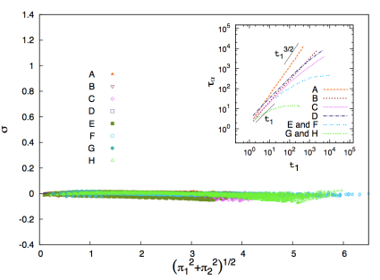
Figure 1: (Color online) Global $(\sigma,\sqrt{\pi_{1}^{2}+\pi_{2}^{2}})$ pairs for all data sets and all possible times $t_{1}<t_{2}<t_{3}$. Inset: Relaxation time $\tau_{\alpha}(t_{1})$ as a function of the waiting time $t_{1}$ for all the models and temperatures considered. $\tau_{\alpha}(t_{1})$ is defined by the condition $C(t_{1}+\tau_{\alpha}(t_{1}),t_{1})=1/e$.

As mentioned in the previous section, if Eq. (1) is satisfied, we expect the local quantities to satisfy $\sigma_{\vec{r}}=0$. In Fig. 2 we show the results of plotting for all systems the 2D projection of the joint probability density of the coarse-grained local correlations, $\rho(|\Delta\sigma_{\vec{r}}|,|\Delta\pi_{\vec{r}}|)$, with $|\Delta\sigma_{\vec{r}}|\equiv|\sigma_{\vec{r}}-\sigma|$ and $|\Delta\pi_{\vec{r}}|\equiv\sqrt{(\pi_{1,{\vec{r}}}-\pi_{1})^{2}+(\pi_{2,{\vec{r}}}-\pi_{2})^{2}}$. The values of the global quantities are subtracted from the local quantities to avoid trivial effects due to differences in the global values. By doing this we are able to better compare the contours independently of the choice of $C(t_{2},t_{1})$ and $C(t_{3},t_{2})$. We do, however, keep the value of $C(t_{3},t_{1})$ approximately the same for all systems, in this case $C(t_{3},t_{1})\approx 0.23$. The three contours shown for each dataset enclose respectively $25\%$, $50\%$, and $75\%$ of the total probability. We coarse grain over moderately large regions, containing on average 125 particles, in order to detect collective fluctuations and, since time reparametrization symmetry is a long time asymptotic effect, we choose the times as late as possible. As the time reparametrization hypothesis predicts, for data sets with $T<T_{c}$ (A–D), the purely longitudinal fluctuations ${\Delta\sigma_{\vec{r}}}$ are clearly smaller than the $\Delta\vec{\pi}_{\vec{r}}$ fluctuations, which contain both transverse and longitudinal contributions. This behavior is more noticeable for the $25\%$ contour, which encloses the most likely fluctuations, than for the $50\%$ and $75\%$ contours. For moderately higher temperature, $T/T_{c}\approx 1.1$ (data sets E and F), the anisotropy $|\Delta\sigma_{\vec{r}}|<|\Delta\vec{\pi}_{\vec{r}}|$ is still present, but less pronounced. In the case of the highest temperature, $T/T_{c}\approx 1.5$ (data sets G and H), the anisotropy is either very slight, or absent. In the case of the systems that are equilibrated, F and H, we find that the shapes of their contours are similar but slightly more anisotropic then the ones obtained for the same temperature in the aging regime, E and G, respectively. The effect of temperature in the anisotropy of the contours can be observed in more detail in Fig. 3(a) where the $25\%$ contour of the probability density for the systems of particles with WCA interactions is shown for three temperatures (data sets D, E, G). This can be directly connected to the fact that, as the temperature is increased, the separation of timescales is less pronounced, the finite time corrections to the time reparametrization symmetry become larger, and the effects of local time variable fluctuations become weaker. The same trends can be observed in Figs. 3(b) and 3(c) for the same datasets as in Fig. 3(a) but for different values of the global correlation $C(t_{3},t_{1})$.

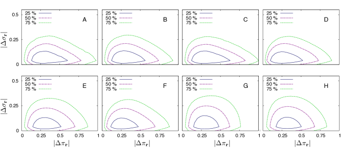
Figure 2: (Color online) 2D contours of constant joint probability density $\rho(|\Delta\sigma_{\vec{r}}|,|\Delta\pi_{\vec{r}}|)$, computed using coarse graining boxes containing 125 particles on average. By subtracting the global quantities to the local quantities we avoid trivial effects due to differences in the global values. Each panel from A to H contains results from the corresponding dataset, for $C(t_{3},t_{1})\approx 0.23$, with the times chosen as late as possible within each dataset. Each set of three concentric contours is chosen so that they enclose $25\%,50\%$, and $75\%$ of the total probability.

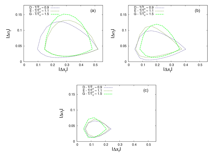
Figure 3: (Color online) Comparison of the contours enclosing $25\%$ of the probability for the aging WCA systems at three different temperatures (D, E, and G). The three different panels correspond to different values of $C(t_{3},t_{1})$: (a) $C(t_{3},t_{1})\approx 0.23$, which is the same value as in Fig. 2, (b) $C(t_{3},t_{1})\approx 0.33$, and (c) $C(t_{3},t_{1})\approx 0.44$.

We can further analyze the effects of choosing different conditions from the ones chosen in Fig. 2, for instance, by comparing the results shown in Fig. 2 with results obtained for smaller coarse graining regions or for shorter times in the aging regime. Exactly this kind of comparison is shown in Fig. 4, where the $25\%$ probability contours for dataset B are shown for three conditions. The contour labeled B is the one shown already in Fig. 2. The contour labeled B’ corresponds to the same time, but with coarse graining regions containing on average 23 particles instead of 125. This leads to less averaging and stronger fluctuations, but also, since fluctuations correlated over shorter distances are no longer preferentially suppressed, the shape of the contour is no longer dominated by collective modes, and thus contour B’ extends more in the direction of $|\Delta\sigma_{\vec{r}}|$ than contour B. The contour labeled B” corresponds to the same coarse graining size of contour B, but with much shorter times. This leads to stronger finite time effects, analogous to the ones found at slightly higher temperatures, and as expected the contour is less anisotropic, and indeed, it resembles the contours corresponding to $T/T_{c}\approx 1.1$.

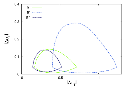
Figure 4: (Color online) $25\%$ probability contours for dataset B with $C(t_{3},t_{1})\approx 0.23$. Contour B corresponds to the $25\%$ of the probability density shown in Fig. 2. Contour B’ corresponds to the same times as contour B, but with a much smaller coarse graining size. Contour label B” corresponds to the same coarse graining size as B, but with much shorter times.

We now move to a more quantitative analysis of the strength and spatial correlations of the fluctuations by making use of the results derived in Sec. II. In Fig. 5(a) we show the ratio between the variances of local transverse fluctuations and longitudinal fluctuations, $\left\langle(\delta\pi_{1,{\vec{r}}}{}^{T})^{2}+(\delta\pi_{2,{\vec{r}}}{}^{T})^{2}\right\rangle/\left\langle(\delta\sigma_{\vec{r}})^{2}\right\rangle$ (“variance anisotropy ratio”) [see Eq. (27)], as a function of the initial time $t_{1}$.

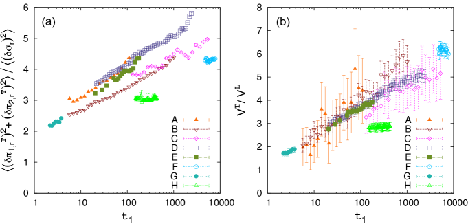
Figure 5: (Color online) (a) Ratio between the variances of transverse and longitudinal fluctuations as a function of the initial time $t_{1}$, for $C(t_{3},t_{1})\approx 0.23$. (b) Ratio between the correlation volumes of transverse and longitudinal fluctuations as a function of $t_{1}$, for the value $C(t_{3},t_{1})\approx 0.23$.

Similarly, in Fig. 5(b) we plot the ratio between the correlation volumes of transverse and longitudinal fluctuations, $V^{T}/V^{L}$ (“correlation volume anisotropy ratio”) [see Eqs. (29) and (30)], also as a function of $t_{1}$. We find that for aging systems both ratios grow as $t_{1}$ increases, as one could expect from the fact that at later times the reparametrizations symmetry breaking terms in the action should become progressively weaker Chamon2002 . For the equilibrium datasets, the dynamics is time translation invariant (TTI), and we observe, as expected, that both anisotropies are independent of $t_{1}$. In Fig. 6, we show the same two ratios as functions of the strength of the dynamical heterogeneities, measured by the dynamical susceptibility $\chi_{4}(t_{3},t_{1})\equiv\chi_{4,C_{31}}=N\left[\left\langle\overline{C_{31}}^{2}\right\rangle-\left\langle\overline{C_{31}}\right\rangle^{2}\right]$. We observe that both anisotropy ratios grow when $\chi_{4,C_{31}}$ increases, i.e., as the dynamical heterogeneity becomes more pronounced. Although the same qualitative behavior is observed for all datasets, the curves are different for different systems and temperatures.

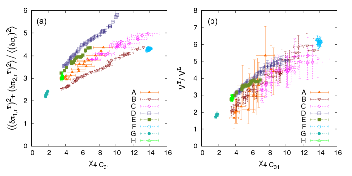
Figure 6: (Color online) (a) Ratio between the variances of transverse and longitudinal fluctuations as a function of the strength of the dynamical heterogeneity, measured by $\chi_{4,C_{31}}\equiv\chi_{4}(t_{3},t_{1})$, for the value $C(t_{3},t_{1})\approx 0.23$. (b) Ratio between the correlation volumes of transverse and longitudinal fluctuations as a function of $\chi_{4,C_{31}}$, for $C(t_{3},t_{1})\approx 0.23$.

The results presented in Fig. 6 correspond to the value $C(t_{3},t_{1})\approx 0.23$, but similar results can be obtained for different values of $C(t_{3},t_{1})$, as one can expect from Fig. 3. Results for three different values of $C(t_{3},t_{1})$ are shown in Fig. 7, where the variance anisotropy ratio for datasets B and D is plotted as a function of $\chi_{4,C_{31}}$ for the values $C(t_{3},t_{1})\approx$ $0.23$, $0.33$, and $0.44$. This figure shows that the variance anisotropy ratio grows with the strength of the dynamical heterogeneity, for all three fixed values of $C(t_{3},t_{1})$.

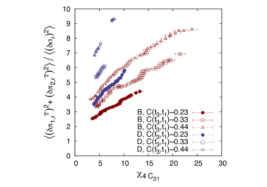
Figure 7: (Color online) Ratio between the variances of transverse and longitudinal fluctuations as a function of $\chi_{4,C_{31}}$, for systems B and D for the values $C(t_{3},t_{1})\approx 0.23$, $0.33$, and $0.44$.

According to the hypothesis, dynamical heterogeneity originates in the Goldstone modes associated to fluctuations in the time reparametrization [see Eq. (4)]. Therefore, the hypothesis implies that the correlation volume of the dynamical heterogeneity should be similar to the correlation volumes of the transverse components of the variables $\pi_{1}$ and $\pi_{2}$, and the longitudinal variable $\sigma$ should be less correlated in space. Our results, shown in Fig. 8, show that this is indeed the case. The correlation volume corresponding to the transverse fluctuations, $V^{T}$, closely tracks the one corresponding to the dynamical heterogeneities, $V_{C_{31}}$, and they both grow together as the temperature is reduced or the timescale is increased. By contrast, for the longitudinal fluctuations $\sigma$ we find that their correlation volume $V^{L}$ is small and essentially constant; it does not correlate with the correlation volume of the dynamical heterogeneity, nor with the temperature or the time scale. In fact, despite the large error bars and the presence of some outlier points, the figure shows a partial data collapse between different systems, both for the case of transverse and for the case of longitudinal correlation volumes. In the case of longitudinal fluctuations, this may be a trivial effect due to the correlation volumes being smaller than the volume of the coarse graining regions used to define the variables. In the case of the transverse fluctuations, the correlation volumes go well beyond the volume of the coarse graining regions, and the partial collapse in the results might be evidence of some sort of universality, but more work will be needed in order to decide this question one way or another.

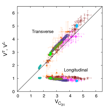
Figure 8: (Color online) Correlation volumes for transverse and longitudinal fluctuations, plotted against $V_{C_{31}}$, the correlation volume for the fluctuations of $C_{31,{\vec{r}}}$, calculated for the value $C(t_{3},t_{1})\approx 0.23$.

IV Conclusions

In this paper we tested the hypothesis that dynamical heterogeneity arises from Goldstone modes related to a broken continuous symmetry under time reparametrizations. In other words, we tested whether dynamical heterogeneity is associated with the presence of spatially correlated fluctuations in the time variables. To verify this, we studied probability distributions that allowed us to distinguish between time reparametrization fluctuations (transverse fluctuations) and other fluctuations (longitudinal fluctuations). We also tested for possible correlations of both the strength and the correlation volume of the fluctuations in the time variable with the dynamical susceptibility $\chi_{4}$, which is normally used to probe dynamical heterogeneity. Altogether, we found that at the lowest temperatures, for the longest timescales and for the largest coarse graining lengths, the transverse fluctuations became stronger than the longitudinal fluctuations, which is consistent with the hypothesis. We also found that the correlation volumes of the time reparametrization fluctuations were proportional to the correlation volume of the dynamical heterogeneity, while the correlation volumes of the longitudinal fluctuations were small and independent of the correlation volumes of the dynamical heterogeneity. These observations apply to all the systems examined, regardless of the details of the interaction (purely repulsive in the case of WCA vs. repulsive and attractive in the case of LJ), the kinds of objects (binary systems of particles vs. systems of short polymers), or the ensembles used in the simulations (NVT vs. NPT). All of this was despite the fact that, to simplify the analysis, we imposed some extra conditions on the form of the correlations, which may have made the agreement with the hypothesis appear less good than it would have been otherwise.

With regards to universality, the evidence we found was mixed. On the one hand, there were clear differences in the details of the results for different systems, for example for the anisotropy ratios. On the other hand, all the trends we observed were the same across systems, and the results for the correlation volumes did show some hints of universality, although the relatively large noise in this measurement did not allow for definite conclusions to be drawn. In any case, the commonality in the results is strong enough to suggest that other systems may display similar qualitative behaviors. Thus, we expect that it would be very instructive to apply the same kind of test to data from other slowly relaxing systems, such as particle tracking data from glassy colloids Kegel2000 ; Weeks2000 ; Weeks2002 ; Courtland2003 and from granular systems close to jamming Keys2007 ; Abate2007 .

Finally, considering the success of the tests presented here, it becomes natural to ask if it is possible to extract from the data the actual fluctuating reparametrization $\phi_{\vec{r}}(t)$, and to study its properties directly. In fact, Ref. Mavimbela shows that some progress can be made in that direction.

V Acknowledgments

H.E.C. thanks E. Flenner, M. Kennett, G. Szamel, and E. Weeks for discussions and C. Chamon and L. Cugliandolo for suggestions and for many discussions. This work was supported in part by the DOE under grant no. DE-FG02-06ER46300, by NSF under grants no. PHY99-07949 and PHY05-51164, and by Ohio University. Karina Avila acknowledges the Condensed Matter and Surface Sciences (CMSS) program for a studentship. Numerical simulations were carried out at the Ohio Supercomputing Center. H.E.C. acknowledges the hospitality of the Aspen Center for Physics and the Kavli Institute for Theoretical Physics, where parts of this work were performed.

References

- (1) P. G. Debenedetti and F. H. Stillinger, Nature 410, 259 (2001).
- (2) M. D. Ediger, Annu. Rev. Phys. Chem. 51, 99 (2000).
- (3) H. Sillescu, J. Non-Crystal. Solids 243, 81 (1999).
- (4) L. Berthier, G. Biroli, J.-P. Bouchaud, L. Cipelletti, and W. van Saarloos, Dynamical heterogeneities in glasses, colloids and granular materials (Oxford University Press, Oxford, 2011).
- (5) N. Lačević, F. W. Starr, T. B. Schröder, and S. C. Glotzer, J. Chem. Phys. 119, 7372 (2003).
- (6) E. Vidal Russell, N. E. Israeloff, L. E. Walther, and H. Alvarez Gomariz, Phys. Rev. Lett. 81, 1461 (1998).
- (7) L. E. Walther, N. E. Israeloff, E. Vidal Russell, and H. Alvarez Gomariz, Phys. Rev. B 57, pp. R15112, 1998.
- (8) E. Vidal Russell, and N. E. Israeloff, Nature 408, 695 (2000).
- (9) W. K. Kegel and A. van Blaaderen, Science 287, 290 (2000).
- (10) E. R. Weeks, J. C. Crocker, A. C. Levitt, A. B. Schofield, and D. A. Weitz, Science 287, 627 (2000).
- (11) E. R. Weeks, and D. A. Weitz, Phys. Rev. Lett. 89, 095704 (2002).
- (12) R. E. Courtland and E. R. Weeks, J Phys Condens. Matter 15, S359 (2003).
- (13) L. Cipelletti, H. Bissig, V. Trappe, P. Ballesta, and. S. Mazoyer, J. Phys. Condens. Matter 15, S257 (2003).
- (14) A. S. Keys, A. R. Abate, S. C. Glotzer, and D. J. Durian, Nature Physics 3, 260, (2007).
- (15) A. R. Abate, and D. J. Durian, Phys. Rev. E 76, 021306 (2007).
- (16) A. Duri, D. A. Sessoms, V. Trappe, and L. Cipelletti, Phys. Rev. Lett. 102 085702 (2009).
- (17) C. Toninelli, M. Wyart, L. Berthier, G. Biroli, and J.-P. Bouchaud, Phys. Rev. E 71, 041505 (2005).
- (18) J. P. Garrahan and D. Chandler, Phys. Rev. Lett. 89, 035704 (2002).
- (19) V. Lubchenko and P. G. Wolynes, Annu. Rev. Phys. Chem. 58, 235 (2007).
- (20) H. E. Castillo, C. Chamon, L. F. Cugliandolo, J. L. Iguain, and M. P. Kennett, Phys. Rev. B 68, 134442 (2003).
- (21) C. Chamon, M. P. Kennett, H. E. Castillo, and L. F. Cugliandolo, Phys. Rev. Lett. 89, 217201 (2002).
- (22) H. E. Castillo, C. Chamon, L. F. Cugliandolo, and M. P. Kennett, Phys. Rev. Lett. 88, 237201 (2002).
- (23) C. Chamon, P. Charbonneau, L. F. Cugliandolo, D. R. Reichman, and M. Sellitto, J. Chem. Phys. 121, 10120 (2004).
- (24) C. Chamon, and L. F. Cugliandolo, J. Stat. Mech. (2007) P07022.
- (25) H. E. Castillo, Phys. Rev. B 78, 214430 (2008).
- (26) G. A. Mavimbela and H. E. Castillo, J. Stat. Mech. (2011) P05017.
- (27) S. Franz, G. Parisi, F. Ricci-Tersenghi and T. Rizzo arXiv:1008.0996 (2010).
- (28) S. Franz, G. Parisi, F. Ricci-Tersenghi and T. Rizzo, Eur. Phys. J. E 34, 102 (2011).
- (29) H. E. Castillo and A. Parsaeian, Nature Physics 3, 26 (2007).
- (30) A. Parsaeian and H. E. Castillo, Phys. Rev. E 78, 060105(R) (2008).
- (31) A. Parsaeian and H. E. Castillo, Phys. Rev. Lett. 102, 055704 (2009).
- (32) A. Parsaeian and H. E. Castillo, arXiv:0811.3190(2008).
- (33) K. E. Avila, H. E. Castillo, and A. Parsaeian, Phys. Rev. Lett. 107, 265702 (2011).
- (34) G. A. Mavimbela, H. E. Castillo, and A. Parsaeian, arXiv:1210.1249 (2012).
- (35) J. P. Bouchaud, L. F. Cugliandolo, J. Kurchan, and M. Mézard. A. P. Young, Spin Glasses and Random Fields (World Scientific, 1998).
- (36) Our notation differs from the one used in Avila . Here, we use instead of . This corresponds to the changes of variables and . Also, in this work, our definition of corresponds to the logarithm of the definition of used in Avila .
- (37) For a slightly different approach to describe fluctuations, centered on extracting the one-time quantities , see Ref. Mavimbela .
- (38) U. Bengtzelius, W. Götze, and A. Sjölander, J. Phys. C 17, 5915 (1984).
- (39) W. Kob and H. C. Andersen, Phys. Rev. E. 52, 4134 (1995).
- (40) D. Chandler, J. D. Weeks, and H. C. Andersen, Science 20, 787 (1983).