Linear Kinetic Coupling of Firehose (KAW) and Mirror Mode

Abstract

A general gyrokinetic dispersion relation is gotten and is applied to analysis linear kinetic coupling of anisotropic firehose (or, kinetic Alfvén wave) and mirror mode. Nyquist stability analysis is also given.

I Introduction

Firehose (FH) and Mirror Mode (MM) instabilities are both pressure anisotropic instabilities, which mainly happen in high beta plasma, and have many applications in space and astrophysical physics. One (FH) happens when parallel pressure exceeding perpendicular one, and the other (MM) happens when perpendicular pressure exceeding parallel one. Both of these two modes have been discussed in literatures by many authors. The basic properties of them can also be found in textbooks or monographs, see e.g., Hasegawa1975a and Treumann1997 .

Mirror mode (MM) instability was identified and discussed since Rudakov1961 , where the MHD theory is used, which is only suitable for long wavelength limit. Tajiri1967 gives a kinetic description, and shows that this mode is not a simply fluid instability. Hasegawa1969 put forward to both the effects of finite Larmor radius (FLR) and nonuniform, i.e., drift-mirror mode. Southwood1993 gives a discussion of the physical mechanism of the linear mirror instability in cold electron temperature limit. Recently, series papers by Pokhotelov et al addressed many details of MM via both fluid theory and kinetic theory, such as finite electron temperature effects Pokhotelov2000 , non-Maxwellian velocity distribution Pokhotelov2002 , finite ion-Larmor radius wavelengths Pokhotelov2004 ; Pokhotelov2006 . Gyrokinetic theory and simulation are introduced to discuss linear and nonlinear MM by Qu et al, Qu2007 ; Qu2008 ; Qu2008a .

Firehose instability is another well-known plasma instability, which is in fact from the same branch of the kinetic Alfven wave (KAW), hence, we will not distinguish them in the following sections. When isotropic but with FLR, we get KAW Hasegawa1975 ; Hasegawa1976 ; while, when anisotropic but using long wavelength limit, we get the classical FH Rosenbluth1956 ; Chandrasekhar1958 ; Parker1958 . It is found by Yoon1993 (also a review paper Yoon1995 ) that a significant new effect which had been neglected in the past will be brought in when allowing the ion gyroradius to be finite. Chen2010 extends Yoon1993 to discuss electron temperature anisotropy effects.

FH and MM have been discussed in almost the same approaches due to their similarities, e.g., CGL fluid, kinetic corrections. However, most the analytical solutions are reduced to just including one of them, and then, there are few discussions of coupling effects. For examples, when mirror mode is unstable, where is the FH (KAW) solution? Can FH be also excited to unstable? Can FH bring MM from a pure damping/growth mode to with real frequency? Schekochihin2008 just discusses the nonlinear growth of FH and mirror fluctuations, mainly via simulation. Duhau1985 has discussed the coupling indeed, but uses the fluid theory then not general. The gyrokinetic treatment of the stability of coupled Alfvén and drift mirror modes in non-uniform plasma can be found in Klimushkin2011 ; Klimushkin2012 , however, where FLR effects are neglected.

Here, we talk about linear coupling effects to answer the above questions. Firstly, a general anisotropic (bi-Maxwellian) 3-by-3 dispersion relation matrix is derived in gyrokinetic framework (then, with FLR effects but only for ${k_{\parallel}}/{k_{\bot}}\ll 1$) in Sec.II. In Sec.III, we show the gyrokinetic dispersion relation can reproduce the FH and MM solutions. In Sec.IV, using only cold electron assumption ${T_{e}}/{T_{i}}\ll 1$, the matrix is reduced to 2-by-2 for discussion the coupling of FH and MM. The dispersion relation is solved both analytical and numerical, and is also compared with the full-kinetic code WHAMP (Waves in Homogeneous Anisotropic Multicomponent Magnetized Plasma, Ronnmark1983 ). General stability properties for arbitrary Larmor radius at the $({\beta_{\parallel}},{\beta_{\bot}})$ plane are made clearly from both analytical and numerical solutions and are also confirmed by Nyquist analysis in Sec.V. A summary is drawn in the last section. Appendix gives some detailed discussions of the gyrokinetic dispersion matrix.

II Gyrokinetic Dispersion Relation Matrix

Here, we use the gyrokinetic (GK) theory Brizard2007 instead of the full kinetic (FK) theory to calculate the general dispersion relation matrix, which excludes the high frequency (${\Omega_{ci}}$ ) modes automatically. The linear GK ordering is

1. Small amplitude: $\delta f/{F_{0}}\sim e\delta\varphi/T\sim\delta B/{B_{0}}\sim\delta\ll 1$;

2. Low frequency: $\omega/{\Omega_{i}}\sim\delta$;

3. Anisotropic: ${k_{\parallel}}/{k_{\bot}}\sim{\rho_{i}}/{L_{0}}\sim\delta,~{}{k_{\bot}}{\rho_{i}}\sim 1$.

For detailed discussion of the gyrokinetic assumptions, one can refer to Brizard2007 or Howes2006 . We comment here, the same ordering $\delta$ used here for all small variables is just for convenience, and the third assumption ${k_{\bot}}{\rho_{i}}\sim 1$ is not a must.

Electrons and ions are assumed both bi-Maxwellian distribution,

$${F_{0}}={1\over{{\pi^{3/2}}\alpha_{\bot}^{2}{\alpha_{\parallel}}}}\exp\left({-{{v_{\bot}^{2}}\over{\alpha_{\bot}^{2}}}-{{v_{\parallel}^{2}}\over{\alpha_{\parallel}^{2}}}}\right),~{}{\alpha_{\bot,\parallel}}={\left({{{2{T_{\bot,\parallel}}}\over m}}\right)^{1/2}}.$$ (1)

Using the framework of Chen1991 , we write the linearized equations of quasi-neutrality condition, vorticity equation (or parallel Ampere’s law) and perpendicular Ampere’s law to matrix form

$$\mathord{\buildrel\lower 3.0pt\hbox{$\scriptscriptstyle\leftrightarrow$}\over{C}}\left[\begin{array}[]{c}\delta{\phi_{\parallel}}\cr\delta\psi\cr{{\delta{B_{\parallel}}}\over{{B_{0}}}}{{{T_{\bot i}}}\over{{q_{i}}}}\end{array}\right]\equiv\left({\begin{array}[]{ccc}{{c_{SS}}}&{{c_{AS}}}&{{c_{MS}}}\cr{{c_{SA}}}&{{c_{AA}}}&{{c_{MA}}}\cr{{c_{SM}}}&{{c_{AM}}}&{{c_{MM}}}\cr\end{array}}\right)\left[\begin{array}[]{c}\delta{\phi_{\parallel}}\cr\delta\psi\cr{{\delta{B_{\parallel}}}\over{{B_{0}}}}{{{T_{\bot i}}}\over{{q_{i}}}}\end{array}\right]=0.$$ (2)

Here, Coulomb gauge $\nabla\cdot\mathbf{A}=0$ is used. $\delta\phi$ is the perturbed electrostatic potential, $\delta\psi=\delta{A_{\parallel}}\cdot\omega/c{k_{\parallel}}$ is a quantity related to the parallel component of the perturbed magnetic vector potential, and $\delta{B_{\parallel}}$ is the parallel component of the perturbed magnetic field. The final dispersion matrix can be gotten as,

$$\mathord{\buildrel\lower 3.0pt\hbox{$\scriptscriptstyle\leftrightarrow$}\over{C}}\equiv\left({\begin{array}[]{ccc}{{c_{SS}}}&{{c_{AS}}}&{{c_{MS}}}\cr{{c_{SA}}}&{{c_{AA}}}&{{c_{MA}}}\cr{{c_{SM}}}&{{c_{AM}}}&{{c_{MM}}}\cr\end{array}}\right)$$ (6)

$$=\left({\begin{array}[]{ccc}{-{\lambda_{1}}+{\lambda_{2}}}&{-{\eta_{i}}{\lambda_{5}}}&{-{\lambda_{3}}-{\lambda_{4}}}\cr{-{\eta_{i}}{\lambda_{5}}}&{{{{\eta_{i}}{b_{i}}}\over{{{\bar{\omega}}^{2}}}}(1+\Delta)-{\eta_{i}}{\lambda_{5}}}&{{\eta_{i}}{\lambda_{6}}}\cr{-{\lambda_{3}}-{\lambda_{4}}}&{{\eta_{i}}{\lambda_{6}}}&{{{2{\eta_{i}}}\over{{\beta_{\bot i}}}}-{\lambda_{7}}-{\lambda_{8}}}\cr\end{array}}\right)$$ (10)

where,

$$\Delta={{{\beta_{\bot i}}}\over{2{b_{i}}}}\left({1-{\eta_{i}}}\right)\left[{1-{\Gamma_{0}}({b_{i}})}\right]+{{{\beta_{\bot e}}}\over{2{b_{e}}}}\left({1-{\eta_{e}}}\right)\left[{1-{\Gamma_{0}}({b_{e}})}\right],$$

$${\lambda_{1}}=\left[{1+{\xi_{i}}Z({\xi_{i}}){\Gamma_{0}}({b_{i}})}\right]+\tau\left[{1+{\xi_{e}}Z({\xi_{e}}){\Gamma_{0}}({b_{e}})}\right],$$

$${\lambda_{2}}=\left({1-{\eta_{i}}}\right)\left[{1-{\Gamma_{0}}({b_{i}})}\right]+\tau\left({1-{\eta_{e}}}\right)\left[{1-{\Gamma_{0}}({b_{e}})}\right],$$

$${\lambda_{3}}=\left({1-{\eta_{i}}}\right){\Gamma_{1}}({b_{i}})-{{{\eta_{i}}}\over{{\eta_{e}}}}\left({1-{\eta_{e}}}\right){\Gamma_{1}}({b_{e}}),$$

$${\lambda_{4}}={\xi_{i}}Z({\xi_{i}}){\Gamma_{1}}({b_{i}})-{{{\eta_{i}}}\over{{\eta_{e}}}}{\xi_{e}}Z({\xi_{e}}){\Gamma_{1}}({b_{e}}),$$

$${\lambda_{5}}=\left[{1-{\Gamma_{0}}({b_{i}})}\right]+{\tau_{\bot}}\left[{1-{\Gamma_{0}}({b_{e}})}\right],$$

$${\lambda_{6}}={\Gamma_{1}}({b_{i}})-{\Gamma_{1}}({b_{e}}),$$

$${\lambda_{7}}=(1-{\eta_{i}}){\Gamma_{2}}({b_{i}})+{{{\eta_{i}}}\over{{\eta_{e}}{\tau_{\bot}}}}(1-{\eta_{e}}){\Gamma_{2}}({b_{e}}),$$

$${\lambda_{8}}={\xi_{i}}Z({\xi_{i}}){\Gamma_{2}}({b_{i}})+{{{\eta_{i}}}\over{{\eta_{e}}{\tau_{\bot}}}}{\xi_{e}}Z({\xi_{e}}){\Gamma_{2}}({b_{e}}),$$

and,

$$\eta\equiv{{{T_{\parallel}}}\over{{T_{\bot}}}},~{}\tau\equiv{{{T_{\parallel i}}}\over{{T_{\parallel e}}}},{\rm{}}{\tau_{\bot}}\equiv{{{T_{\bot i}}}\over{{T_{\bot e}}}},~{}\beta\equiv{{8\pi{n_{0}}T}\over{B_{0}^{2}}},$$

$$b\equiv{{k_{\bot}^{2}{\rho^{2}}}\over 2},{\rm{}}{\bar{\omega}^{2}}\equiv{{{\omega^{2}}}\over{k_{\parallel}^{2}v_{A}^{2}}},$$

$$\delta{\phi_{\parallel}}\equiv\delta\phi-\delta\psi~{}({E_{\parallel}}=-i{k_{\parallel}}\delta{\phi_{\parallel}}),$$

$${\Gamma_{0}}(b)={I_{0}}(b){e^{-b}},$$

$${\Gamma_{1}}(b)=\left[{{I_{0}}(b)-{I_{1}}(b)}\right]{e^{-b}},{\rm{}}{\Gamma_{2}}(b)=2{\Gamma_{1}}(b).$$

where ${I_{n}}$ is the first kind modified Bessel function. The dispersion relation is

$$\det\left|{\mathord{\buildrel\lower 3.0pt\hbox{$\scriptscriptstyle\leftrightarrow$}\over{C}}}\right|=0$$ (11)

We see from (6), the matrix is symmetrical, i.e., $c_{AS}=c_{SA}$, $c_{AM}=c_{MA}$ and $c_{MS}=c_{SM}$, which is similar with the full-kinetic one (see e.g., Stix1992 ). When isotopic ($\eta_{i,e}=1$), (11) reduces to exactly the same result as Howes2006 . At appendix, we also show that when drop small terms from reduced full-kinetic result in Yoon1993 , it also gives the same result as this gyrokinetic one.

We can see from (6), the solutions for $\bar{\omega}$ is independent of ${k_{\parallel}}$, which means always ${\omega^{2}}\propto k_{\parallel}^{2}$. This is the main drawback of (11) because of that ${k_{\parallel}}/{k_{\bot}}$ is taken as small term and dropped, then not suitable to discuss the fine structures of the dispersion relation, e.g., the maximum growth rate ${\gamma_{\max}}$ of mirror mode. However, one can also add the small terms when necessary by comparing with the full-kinetic result (see appendix). For example, Qu2007 adds a ${k_{\parallel}}/{k_{\bot}}$ term in integral form when discuss mirror mode.

III Solutions of Firehose and Mirror Mode

In (6), when only considering one matrix element, $c_{SS}=0$ gives ions sound wave (ISW, only consider $\delta{\phi_{\parallel}}$), $c_{AA}=0$ gives shear Alfven wave (SAW, only consider $\delta\psi$) and $c_{MM}=0$ gives mirror mode (MM, only consider $\delta{B_{\parallel}}$). $c_{\alpha\beta}(\alpha,\beta=S,A,M)$ is the coupling of each waves.

III.1 Firehose (KAW) Branch

As mentioned above, $c_{AA}=0$ represents the firehose and KAW solution,

$${{\bar{\omega}}^{2}}={{{b_{i}}}\over{{\lambda_{5}}}}(1+\Delta)={{{b_{i}}}\over{\left[{1-{\Gamma_{0}}({b_{i}})}\right]+{\tau_{\bot}}\left[{1-{\Gamma_{0}}({b_{e}})}\right]}}$$

$$\left\{{1+{{{\beta_{\bot i}}}\over{2{b_{i}}}}\left({1-{\eta_{i}}}\right)\left[{1-{\Gamma_{0}}({b_{i}})}\right]+{{{\beta_{\bot e}}}\over{2{b_{e}}}}\left({1-{\eta_{e}}}\right)\left[{1-{\Gamma_{0}}({b_{e}})}\right]}\right\}.$$ (12)

When small Lamor radius ${b_{e}}\ll{b_{i}}\ll 1$, ${\Gamma_{0}}(b)\simeq 1-b+3{b^{2}}/4\simeq 1-b$, (III.1) reduces to,

$${\bar{\omega}^{2}}=1+\Delta=1+{{{\beta_{\bot i}}}\over 2}\left({1-{\eta_{i}}}\right)+{{{\beta_{\bot e}}}\over 2}\left({1-{\eta_{e}}}\right),$$ (13)

which is the classical firehose solution, and when $1+\Delta<0$, this mode is unstable. When isotropic ${\eta_{i,e}}=1$, $\Delta=0$, (III.1) reduces to

$${\bar{\omega}^{2}}={{{b_{i}}}\over{\left[{1-{\Gamma_{0}}({b_{i}})}\right]+{\tau_{\bot}}\left[{1-{\Gamma_{0}}({b_{e}})}\right]}},$$ (14)

Still using the small Lamor radius assumption to go further, (14) reduces to

$${\bar{\omega}^{2}}=1+3{b_{i}}/4,$$ (15)

(15) is the classical KAW solution Hasegawa1975 ; Hasegawa1976 .

III.2 Mirror Mode Branch

At this case, $c_{MM}=0$, gives

$${{2{\eta_{i}}}\over{{\beta_{\bot i}}}}-{\lambda_{7}}-{\lambda_{8}}=0,$$ (16)

And, dropping the contributions from electrons (cold electrons assumption) in (16), gives,

$${\xi_{i}}Z({\xi_{i}})={{{\eta_{i}}-(1-{\eta_{i}}){\Gamma_{1}}({b_{i}}){\beta_{\bot i}}}\over{{\beta_{\bot i}}{\Gamma_{1}}({b_{i}})}}.$$ (17)

(17) is the mirror mode solution. Qu2007 adds a ${k_{\parallel}}/{k_{\bot}}$ term to (17), then can be used to discuss the ${\gamma_{\max}}$ of mirror mode, which give the same result as Pokhotelov2004 from full-kinetic theory.

IV Coupling of Firehose and Mirror Mode

In the above section, we use only one matrix element of the 3-by-3 general dispersion matrix (6), then get kinetic version of both FH (KAW) and MM, which shows accurately enough to discuss single mode by compared with full-kinetic results from previous authors.

At this section, we solve the 2-by-2 matrix to discuss coupling effects of FH and MM. The matrix (6) is general for arbitrary $b_{i,e}$, $\beta_{i,e}$, ${\xi_{i,e}}$ under the gyrokinetic ordering. When cold electrons ($T_{e}/T_{i}\ll 1$), we have $b_{e}\ll 1$, $\tau,{\tau_{\bot}}\gg 1$, ${c_{SS}}\gg{c_{SA}},{c_{SM}}$, then $\delta{\phi_{\parallel}}$ should be very small, which means the parallel electrical field is short circuited (few percents of cold electrons in density is enough, see Hasegawa1975a ). We use this only assumption to reduce the 3-by-3 matrix to 2-by-2 for discussion FH and MM coupling.

(11) reduces to,

$$\left|\begin{array}[]{cc}{{{\eta_{i}}{b_{i}}}\over{{{\bar{\omega}}^{2}}}}(1+\Delta)-{\eta_{i}}{\lambda_{5}}&{{\eta_{i}}{\lambda_{6}}}\\ {{\eta_{i}}{\lambda_{6}}}&{{{2{\eta_{i}}}\over{{\beta_{\bot i}}}}-{\lambda_{7}}-{\lambda_{8}}}\end{array}\right|=0,$$ (18)

where,

$$\Delta={{{\beta_{\bot i}}}\over{2{b_{i}}}}\left({1-{\eta_{i}}}\right)\left[{1-{\Gamma_{0}}({b_{i}})}\right]+{{{\beta_{\bot e}}}\over 2}\left({1-{\eta_{e}}}\right)$$

$$\simeq{{{\beta_{\bot i}}}\over 2}\left({1-{\eta_{i}}}\right)(1-{3\over 4}{b_{i}}),$$

$${\lambda_{5}}\simeq 1-{\Gamma_{0}}({b_{i}})\simeq{b_{i}}-{3\over 4}b_{i}^{2},$$

$${\lambda_{6}}\simeq{\Gamma_{1}}({b_{i}})-1\simeq-{3\over 2}{b_{i}}+{5\over 4}b_{i}^{2},$$

$${\lambda_{7}}\simeq 2(1-{\eta_{i}}){\Gamma_{1}}({b_{i}}),$$

$${\lambda_{8}}=2{\xi_{i}}Z({\xi_{i}}){\Gamma_{1}}({b_{i}})+{{2{\eta_{i}}}\over{{\eta_{e}}{\tau_{\bot}}}}{\xi_{e}}Z({\xi_{e}}){\Gamma_{1}}({b_{e}})$$

$$\simeq 2{\xi_{i}}Z({\xi_{i}}){\Gamma_{1}}({b_{i}}).$$ (19)

The small $b_{i}$ expansion is also written in (IV) but only used when necessary.

Pokhotelov2004 has given a very similar 2-by-2 matrix as (18) via full-kinetic theory, which contains also the small ${k_{\parallel}}/{k_{\bot}}$ correction. But, it solves only MM by dropping the firehose correction in the mirror approximation $\left|\omega\right|\ll\left|{{k_{\parallel}}{v_{i,\parallel}}}\right|$. A fluid theory is used to discuss the instability of mirror mode and firehose in Duhau1985 , and several stable and unstable regions are given in different parameters space. Since there is no kinetic effect, the results of Duhau1985 will be unreasonable. Ignoring FLR effects, Klimushkin2012 gives the gyrokinetic treatment of the stability of coupled Alfvén and drift mirror modes in 1D non-uniform plasma.

For analytical tractable, we solve (18) in long wavelength approximation in this section. This means $b_{i}\ll 1$. Keep $O(1)+O(b)$, (18) changes to

$$-\left\{{{{{\eta_{i}}}\over{{\beta_{\bot i}}}}-\left[{(1-{\eta_{i}})+{\xi_{i}}Z({\xi_{i}})}\right]}\right\}\left[{{1\over{{{\bar{\omega}}^{2}}}}(1+\Delta)-1}\right]$$ (20)

$$=\left\{\begin{array}[]{c}{3\over 4}{{{\eta_{i}}}\over{{\beta_{\bot i}}}}-{3\over 4}\left[{(1-{\eta_{i}})+{\xi_{i}}Z({\xi_{i}})}\right]+\\ {3\over 2}\left[{(1-{\eta_{i}})+{\xi_{i}}Z({\xi_{i}})}\right]\left[{{1\over{{{\bar{\omega}}^{2}}}}(1+\Delta)-1}\right]-{9\over 8}{\eta_{i}}\end{array}\right\}{b_{i}}$$ (23)

We use (20) to see the correction from MM to FH and FH to MM.

IV.1 Mirror mode correction to Firehose (KAW)

Look the small FLR correction to firehose solution $\left[{(1+\Delta)/{{\bar{\omega}}^{2}}-1}\right]\sim O({b_{i}})$,

$${\bar{\omega}^{2}}={{(1+\Delta)}\over{1-{{\left\{{{3\over 4}{{{\eta_{i}}}\over{{\beta_{\bot i}}}}-{3\over 4}\left[{(1-{\eta_{i}})+{\xi_{i}}Z({\xi_{i}})}\right]-{9\over 8}{\eta_{i}}}\right\}{b_{i}}}\over{\left\{{{{{\eta_{i}}}\over{{\beta_{\bot i}}}}-\left[{(1-{\eta_{i}})+{\xi_{i}}Z({\xi_{i}})}\right]}\right\}}}}}.$$ (24)

IV.1.1 Cold ions

When cold ions, $\left|\omega\right|\gg\left|{{k_{\parallel}}{v_{i,\parallel}}}\right|$, ${\xi_{i}}=\bar{\omega}/\sqrt{{\beta_{\parallel i}}}\gg 1$, ${\xi_{i}}Z({\xi_{i}})\simeq-1-1/({2\xi_{i}^{2}})\simeq-1$,

$${{\bar{\omega}}^{2}}={{(1+\Delta)}\over{1-{{{3\over 8}\left\{{{2\over{{\beta_{\bot i}}}}-1}\right\}{b_{i}}}\mathord{\left/{\vphantom{{{3\over 8}\left\{{{2\over{{\beta_{\bot i}}}}-1}\right\}{b_{i}}}{\left\{{{1\over{{\beta_{\bot i}}}}+1}\right\}}}}\right.\kern-1.2pt}{\left\{{{1\over{{\beta_{\bot i}}}}+1}\right\}}}}}$$

$$\buildrel{{\eta_{i}}=1,~{}{\rm{}}{\beta_{\bot i}}\ll 1}\over{\Longrightarrow}{{\bar{\omega}}^{2}}\simeq 1+{3\over 4}{b_{i}}~{}{{\rm{(KAW)}}}$$ (25)

IV.1.2 Hot ions

Here, we try to see that, when classical FH (KAW) is stable ( $1+\Delta>0$), whether MM can excite it to unstable. When hot ions, $\left|\omega\right|\ll\left|{{k_{\parallel}}{v_{i,\parallel}}}\right|$, ${\xi_{i}}=\bar{\omega}/\sqrt{{\beta_{\parallel i}}}\ll 1$, ${\xi_{i}}Z({\xi_{i}})\simeq i\sqrt{\pi}{\xi_{i}}=\bar{\omega}{{i\sqrt{\pi}}\mathord{\left/{\vphantom{{i\sqrt{\pi}}{\sqrt{{\beta_{\parallel i}}}}}}\right.}{\sqrt{{\beta_{\parallel i}}}}}\simeq{{i\sqrt{\pi}\sqrt{1+\Delta}{\mathop{\rm sgn}}(\bar{\omega})}\mathord{\left/{\vphantom{{i\sqrt{\pi}\sqrt{1+\Delta}{\mathop{\rm sgn}}(\bar{\omega})}{\sqrt{{\beta_{\parallel i}}}}}}\right.}{\sqrt{{\beta_{\parallel i}}}}}$, (Note: in fact, $\bar{\omega}$ is complex)

$${{\bar{\omega}}^{2}} ={{(1+\Delta)\left\{\begin{array}[]{c}\left[{{A^{2}}-{{3{b_{i}}}\over 4}(A-{3\over 2}{\eta_{i}})A+(1-{{3{b_{i}}}\over 4}){B^{2}}}\right]\\ -\left[{{9\over 8}{b_{i}}{\eta_{i}}B}\right]i\end{array}\right\}}\over{{{\left[{A-{{3{b_{i}}}\over 4}(A-{3\over 2}{\eta_{i}})}\right]}^{2}}+{{\left[{(1-{{3{b_{i}}}\over 4})B}\right]}^{2}}}}$$ (28)

$$=a-i{\mathop{sgn}}(\bar{\omega})b~{}\left({a\sim O(1),~{}b\sim O({b_{i}})}\right)$$ (29)

where,

$$A\equiv{{{\eta_{i}}}\over{{\beta_{\bot i}}}}-(1-{\eta_{i}}),{\rm{}}B\equiv{{\sqrt{\pi}\sqrt{1+\Delta}{\mathop{\rm sgn}}(\bar{\omega})}\over{\sqrt{{\beta_{\parallel i}}}}}$$ (30)

Due to $-{\mathop{\rm sgn}}(\bar{\omega})$, and provided, $a>0$, the solutions are always damped.

To find a unstable mode, which means $a<0$,

$$a<0\Leftrightarrow\underbrace{(1-{{3{b_{i}}}\over 4}){A^{2}}}_{>0}+\underbrace{{9\over 8}{b_{i}}{\eta_{i}}A}_{<0}+\underbrace{(1-{{3{b_{i}}}\over 4}){B^{2}}}_{>0}<0,$$ (31)

(31) can only be satisfied when $A<0$, i.e., mirror mode is unstable. While, if there is a domain satisfy both $a<0$ and $A<0$, there must be at least one point satisfy both $a=0$ and $A=0$,

$$\left\{\begin{array}[]{c}a=0,\hfill\cr A=0,\hfill\cr\end{array}\right.\Leftrightarrow\left\{\begin{array}[]{c}(1-{{3{b_{i}}}\over 4}){B^{2}}=0,\hfill\cr A=0,\hfill\cr\end{array}\right.\Leftrightarrow\left\{\begin{array}[]{c}B=0,\hfill\cr A=0,\hfill\cr\end{array}\right.$$ (38)

$$\Leftrightarrow\left\{\begin{array}[]{c}1+\Delta=0,\hfill\cr{{{\eta_{i}}}\over{{\beta_{\bot i}}}}-(1-{\eta_{i}})=0,\hfill\cr\end{array}\right.$$ (41)

(38) can never be satisfied, then, there is no unstable domain, providing we use small argument expansion of ${\Gamma_{0,1}}({b_{i}})$ and $Z({\xi_{i}})$.

We can also contour plot (see FIG.1) the $a=0$ boundary and $A=0$ boundary to show whether there is a region satisfy both (31) and $A<0$. However, these contour plots can also help to show the sizes of each kind of ranges.

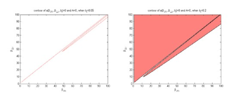
Figure 1: Contour plot of $a=0$ and $A=0$.

We see that, indeed, none of the parameters $({\beta_{\parallel i}},~{}{\beta_{\bot i}})$ satisfy both $a<0$ and $A<0$, which means that the unstable domain, if it exists, should be very very narrow. The only possibility is when ${\Gamma_{0,1}}({b_{i}})$ or $Z({\xi_{i}})$ cannot be expanded, i.e., ${b_{i}}\sim 1$ or ${\xi_{i}}\sim 1$. In next section, we will use Nyquist technique to prove that there is indeed no unstable domain for exciting the classical stable FH (KAW) in arbitrary parameters.

IV.1.3 Numerical solutions

Numerical solutions of (18) at FH (KAW) branch are given below,

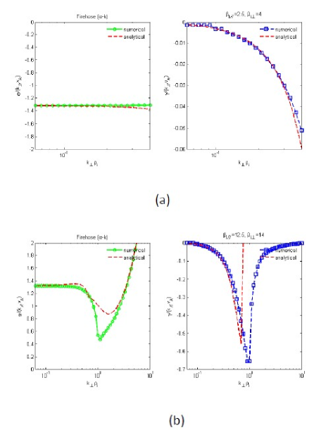
Figure 2: Numerical solution and analytical solution (28), firehose (KAW).

FIG.2 shows, the analytical and numerical solutions are agreed very well. The coupling of MM is weak, and mainly brings KAW (FH) a damping.

IV.2 Firehose correction to mirror mode

At this case,

$$\left[{{{2{\eta_{i}}}\over{{\beta_{\bot i}}}}-{\lambda_{7}}-{\lambda_{8}}}\right]={\eta_{i}}\lambda_{6}^{2}/\left[{{{{b_{i}}}\over{{{\bar{\omega}}^{2}}}}(1+\Delta)-{\lambda_{5}}}\right],$$ (42)

We define ${\bar{\omega}_{0}}$ be the traditional mirror mode solution (zeroth order), i.e., ${\xi_{i0}}={\bar{\omega}_{0}}/\sqrt{{\beta_{\parallel i}}}\ll 1$, and

$${\xi_{i0}}Z({\xi_{i0}})={{{\eta_{i}}-(1-{\eta_{i}}){\Gamma_{1}}({b_{i}}){\beta_{\bot i}}}\over{{\beta_{\bot i}}{\Gamma_{1}}({b_{i}})}},$$ (43)

We can rewrite (42) as,

$${\xi_{i}}Z({\xi_{i}})\simeq\left[{{{{\eta_{i}}}\over{{\beta_{\bot i}}}}-(1-{\eta_{i}})}\right]-{{{\eta_{i}}{{[{\Gamma_{1}}({b_{i}})-1]}^{2}}}\over{2\left\{{{{{b_{i}}}\over{\bar{\omega}_{0}^{2}}}(1+\Delta)-\left[{1-{\Gamma_{0}}({b_{i}})}\right]}\right\}}},$$ (44)

which brings just a very small correction and MM is still pure growing or damped. This means the coupling from KAW (FH) is also weak, and the traditional treatment of MM reasonable. To go further, we use the expansion ${\xi_{i}}Z({\xi_{i}})\simeq i{\xi_{i}}\sqrt{\pi}\left[{{e^{-\xi_{i}^{2}}}-2{\xi_{i}}}\right]\simeq i\sqrt{\pi}\bar{\omega}/\sqrt{{\beta_{\parallel i}}}$. The analytical solution in FIG.3 is by solving (43) and (44) with ${\xi_{i}}Z({\xi_{i}})\simeq i\sqrt{\pi}\bar{\omega}/\sqrt{{\beta_{\parallel i}}}$, and then adding the correction term $\left[{{e^{-\xi_{i}^{2}}}-2{\xi_{i}}}\right]$. Numerical solutions of (18) at mirror mode branch are also given.

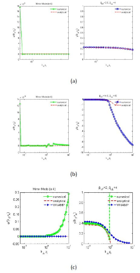
Figure 3: Numerical solution of (18) and analytical solution from (44), mirror mode.

From FIG.3(b), we can see, for mirror mode, the analytical solution is only suitable when ${b_{i}}\ll 1$, because, when ${b_{i}}>\sim 1$, ${\xi_{i}}=\bar{\omega}/\sqrt{{\beta_{\parallel i}}}\sim 1$ . At FIG.3(c), the mirror mode assumption is totally broken when $b_{i}$ is large. WHAMP result is also shown.

IV.3 Physics Mechanism

IV.3.1 Mirror mode to firehose (KAW)

We find from the analytical and numerical solution above, that, the correction from mirror mode to firehose (KAW) is always bring not a unstable but a damping. This seems mean that the mirror cannot excite firehose but, on the contrary, absorb energy from firehose.

It’s widely accepted that the mechanism of mirror mode unstable is both the Landau type (wave-particle resonant) and the anisotropic free energy type. Then, it is physical reasonable that when mirror mode is unstable, it absorbs energy from firehose and cause which damped.

IV.3.2 Firehose to mirror mode

Mirror mode is always pure growing or damping (${\mathop{\rm Re}\nolimits}(\left|{\bar{\omega}}\right|)\ll{\mathop{\rm Im}\nolimits}(\left|{\bar{\omega}}\right|)$), even though with firehose coupling. There is a narrow range (${\beta_{\bot i}}>\sim{\beta_{\parallel i}}$), both mirror mode and firehose are damping, which may be caused by Landau damping, similar with beam-plasma system (a range the free energy of non-Maxwellian distribution cannot compete to Landau damping).

V Nyquist Stabilities Analysis

The dispersion relation (18) can be rewritten as

$$D(\omega)=({\bar{\omega}^{2}}-{\alpha_{0}})({\alpha_{1}}-{\xi_{i}}Z({\xi_{i}}))+{\bar{\omega}^{2}}{c^{2}}=0,$$ (45)

where

$${\alpha_{0}}={{{b_{i}}}\over{1-{\Gamma_{0}}({b_{i}})}}(1+\Delta),{\rm{}}{\alpha_{1}}={{{\eta_{i}}}\over{{\beta_{\bot i}}{\Gamma_{1}}({b_{i}})}}-(1-{\eta_{i}}),$$

$${\rm{}}{c^{2}}={{{\eta_{i}}{{[{\Gamma_{1}}({b_{i}})-1]}^{2}}}\over{2{\Gamma_{1}}({b_{i}})[1-{\Gamma_{0}}({b_{i}})]}}.$$ (46)

Classical results of firehose and mirror mode instabilities,

$${\rm{Firehose:}}~{}\left\{\begin{array}[]{c}{\rm{stable:}}~{}{\alpha_{0}}>0,\hfill\cr{\rm{unstable:}}~{}{\alpha_{0}}<0.\hfill\cr\end{array}\right.;$$ (49)

$${\rm{Mirrormode:}}~{}\left\{\begin{array}[]{c}{\rm{stable:}}~{}{\alpha_{1}}>0,\hfill\cr{\rm{unstable:}}~{}{\alpha_{1}}<0.\hfill\cr\end{array}\right..$$ (52)

For different $({\beta_{\parallel}},{\rm{}}{\beta_{\bot}})$, there are three regions: (1) ${\alpha_{0}}>0,{\rm{}}{\alpha_{1}}<0$, mirror mode unstable region; (2) ${\alpha_{0}}<0,{\rm{}}{\alpha_{1}}>0$, firehose unstable region; (3) ${\alpha_{0}}>0,{\rm{}}{\alpha_{1}}>0$, both stable (damping) region.

V.1 Mirror mode unstable region

We use Nyquist technique to prove that when ${\alpha_{0}}>0,{\rm{}}{\alpha_{1}}<0$(mirror mode unstable region), there is only one unstable mode (i.e., mirror mode).

$${\xi_{i}}Z({\xi_{i}})={\xi_{i}}{Z_{ir}}+i{\xi_{i}}{Z_{ii}},$$ (53)

$$D(\omega)=({\bar{\omega}^{2}}-{\alpha_{0}})({\alpha_{1}}-{\xi_{i}}{Z_{ir}})+{\bar{\omega}^{2}}{c^{2}}-i({\bar{\omega}^{2}}-{\alpha_{0}}){\xi_{i}}{Z_{ii}},$$ (54)

When $\left|\omega\right|\to\infty$,

$$D(\omega)\to{\bar{\omega}^{2}}({\alpha_{1}}+1+{c^{2}})>0,$$ (55)

Along $-\infty<{\omega_{r}}<\infty$, at ${\mathop{\rm Im}\nolimits}D(\omega)=0$

$$\left\{\begin{array}[]{c}{{\bar{\omega}}^{2}}={\alpha_{0}},{\rm{}}D={\alpha_{0}}{c^{2}}>0,\hfill\cr\bar{\omega}=0,{\rm{}}D=-{\alpha_{0}}{\alpha_{1}}>0.\hfill\cr\end{array}\right.$$ (56)

The Nyquist diagram will draw as FIG.4.

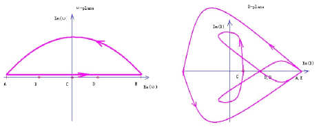
Figure 4: Nyquist diagram of (45), mirror mode unstable region.

We see from FIG.4, the mapping in complex D-plane indeed encircle the origin point, and one time, which means there is indeed only one unstable mode. A numerical result of the mapping (partly) is shown below in FIG.5

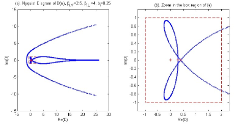
Figure 5: Nyquist diagram of (45) verified by numerical, mirror mode unstable region.

V.2 Firehose unstable region

At this case ${\alpha_{0}}<0,{\rm{}}{\alpha_{1}}>0$. When $\left|\omega\right|\to\infty$, we still have (55). And, along $-\infty<{\omega_{r}}<\infty$, ${\mathop{\rm Im}\nolimits}D(\omega)=0$ at only $\bar{\omega}=0$, which gives $D=-{\alpha_{0}}{\alpha_{1}}>0$. Then, after drawing the Nyquist diagram, we can also get only one unstable mode (i.e., firehose). A result is shown in FIG.6

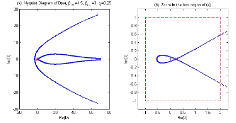
Figure 6: Nyquist diagram of (45) verified by numerical, firehose unstable region.

V.3 Both stable (damping) region

At this case ${\alpha_{0}}>0,{\rm{}}{\alpha_{1}}>0$, the analysis is similar with the mirror mode unstable case, except that in Fig4, the point $C>0$ in $D$-plane should be changed to $C<0$. Then, the mapping in complex D-plane will never encircle the origin point, which means all the solutions are stable. A result is shown in FIG.7

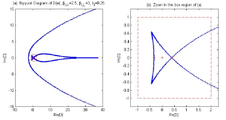
Figure 7: Nyquist diagram of (45) verified by numerical, stable region.

VI Summary

In this paper, we firstly give a general 3-by-3 gyrokinetic dispersion matrix for anisotropic bi-Maxwellain distribution plasma to discuss low-frequency hydromagnetic waves, which is suitable for arbitrary $b_{i,e}$, $\beta_{i,e}$, $\xi_{i,e}$ under the gyrokinetic ordering. This gyrokinetic matrix is useful to discuss various kinetic corrections to hydrodynamica waves. Some detailed solutions are given in Howes2006 for isotropic plasma, e.g., analytical form of high $\beta$ KAW. However, the gyrokinetic matrix can also be extended to arbitrary distribution and arbitrary species, and also to nonuniform plasma. One can do this by following the framework in Chen1991 , see e.g., Klimushkin2012 for 1D nonuniform plasma case. As an application example, we use this dispersion matrix to discuss the coupling of firehose and mirror mode. At the cold electron assumption, the matrix is reduced to 2-by-2, for the coupling of firehose (KAW) and mirror mode. The dispersion relation is solved both analytical and numerical, and shows consistent very well between each other. The results by the kinetic code WHAMP with all kinetic effects also show the reduced dispersion relation is appropriate. We find there exists at most one unstable solution at the $({\beta_{\parallel}},{\rm{}}{\beta_{\bot}})$ plane for arbitrary Lamor radius, and the plane can be divided into three regions: firehose unstable region; mirror mode unstable region; both modes stable (damping) region. The Nyquist analysis confirms these three regions.

VII Acknowledgments

One author, HSX, thanks the discussions with Ling CHEN, Hong-peng QU and Peter. H. YOON, and also thanks Richard E. DENTON for providing the java version of WHAMP.

VIII Appendix

At this appendix, we compare the full-kinetic dispersion relation from Yoon1993 with our gyrokinetic one.

Drop the electrons term as Yoon1993 by assuming $b_{e}\ll 1$, (11) can be rewritten to,

$$[{\eta_{i}}DAC+{\eta_{i}}{\eta_{i}}{E^{2}}A-{\eta_{i}}D{B^{2}}]{\bar{\omega}^{2}}+{\eta_{i}}{b_{i}}(1+\Delta)$$

$$\left[{C({\eta_{i}}D-A)+{{({\eta_{i}}E-B)}^{2}}}\right]=0,$$ (57)

where,

$$\Delta={{{\beta_{\bot i}}}\over{2{b_{i}}}}\left({1-{\eta_{i}}}\right)\left[{1-{\Gamma_{0}}({b_{i}})}\right]+{{{\beta_{\bot e}}}\over 2}\left({1-{\eta_{e}}}\right),$$ (58)

$$A={{Z^{\prime}({\xi_{i}})}\over 2}{\Gamma_{0}}({b_{i}})+\tau{{Z^{\prime}({\xi_{e}})}\over 2},$$ (59)

$$B={{Z^{\prime}({\xi_{i}})}\over 2}{\Gamma_{1}}({b_{i}})-{{{\eta_{i}}}\over{{\eta_{e}}}}{{Z^{\prime}({\xi_{e}})}\over 2},$$ (60)

$$C={{2{\eta_{i}}}\over{{\beta_{\bot i}}}}+2{\eta_{i}}{\Gamma_{1}}({b_{i}})+2{{{\eta_{i}}}\over{{\tau_{\bot}}}}+{{Z^{\prime}({\xi_{i}})}\over 2}{\Gamma_{2}}({b_{i}})+{{{\eta_{i}}}\over{{\eta_{e}}{\tau_{\bot}}}}{{Z^{\prime}({\xi_{e}})}\over 2},$$ (61)

$$D=\left[{1-{\Gamma_{0}}({b_{i}})}\right]={\lambda_{6}},$$ (62)

$$E=\left[{1-{\Gamma_{1}}({b_{i}})}\right]=-{\lambda_{7}}.$$ (63)

Dropping the $O({\delta^{2}})$ term $k_{z}^{2}v_{A}^{2}/\Omega_{i}^{2}$ in Yoon1993 , keep only $O(1)$ term in $\eta$ and $\eta^{\prime}$, the full-kinetic dispersion relation in Yoon1993 can be written as ,

$$\underbrace{-A\varepsilon^{\prime}{{({\omega\over{{\Omega_{i}}}})}^{4}}}_{O({\delta^{4}})}+\underbrace{(2A-{b_{i}}{\eta_{i}})(1+\Delta){{k_{\parallel}^{2}v_{A}^{2}}\over{\Omega_{i}^{2}}}{{({\omega\over{{\Omega_{i}}}})}^{2}}}_{O({\delta^{4}})}$$ (64)

$$+\underbrace{{{k_{\parallel}^{2}v_{A}^{2}}\over{\Omega_{i}^{2}}}(1+\Delta){{k_{\parallel}^{2}v_{A}^{2}}\over{\Omega_{i}^{2}}}(1+\Delta)\left[{\left({{b_{i}}{\eta_{i}}-A}\right)}\right]}_{O({\delta^{4}})}$$ (65)

$$+\underbrace{\left[{{b_{i}}{\eta_{i}}{{AC}\over{{\eta_{i}}}}+A{E^{2}}-{1\over{4{\eta_{i}}}}{b_{i}}{B^{2}}}\right]{{({\omega\over{{\Omega_{i}}}})}^{2}}}_{{b_{i}}O({\delta^{2}})}+$$ (66)

$$\underbrace{{{k_{\parallel}^{2}v_{A}^{2}}\over{\Omega_{i}^{2}}}(1+\Delta){b_{i}}{\eta_{i}}\left[{{1\over{{\eta_{i}}}}C\left({D-{A\over{{\eta_{i}}}}}\right)+{{\left({E-{B\over{2{\eta_{i}}}}}\right)}^{2}}}\right]}_{{b_{i}}O({\delta^{2}})}=0$$ (67)

where,

$$\varepsilon^{\prime}={{1-{I_{0}}{e^{-{\lambda_{i}}}}}\over{{\lambda_{i}}}}-2{\lambda_{i}}\sum\limits_{n=1}^{\infty}{{{2{{\left({{I_{n}}{e^{-{\lambda_{i}}}}}\right)}^{\prime}}}\over{{n^{2}}}}}\sim O(1)$$ (68)

Dropping the high order $O({\delta^{4}})$ terms in (64), we get exactly the same result as the gyrokinetic result (VIII). We find in (64) when ${b_{i}}\sim k_{\parallel}^{2}v_{A}^{2}/\Omega_{i}^{2}$, the ${b_{i}}O({\delta^{2}})$ will jump to $O({\delta^{4}})$!! So, we cannot drop the $O({\delta^{4}})$ in (64) when ${b_{i}}\to 0$. This is what Yoon1993 found.

In Yoon1993 , the classical firehose solution is found in full-kinetic at the $O({\delta^{4}})$ terms, because ${b_{i}}O({\delta^{2}})$ terms can be dropped when ${b_{i}}\to 0\ll O({\delta^{2}})$. While in gyrokinetic, the solution is found in ${b_{i}}O({\delta^{2}})$ terms, because we have ruled out the $O({\delta^{4}})$ terms by gyrokinetic assumptions. It should be just a coincidence that they give the same firehose result. The different can also be explained in another way: to get the classical firehose solution, the full-kinetic approach of Yoon1993 uses the assumption ${b_{i}}\to 0\ll O({\delta^{2}})$, while the gyrokinetic approach uses ${b_{i}}\to 0\gg O({\delta^{2}})$.

To discussion the fine structure of the hydrodynamica waves and instabilities, (64) can be seen as an extent version of our gyrokinetic dispersion relation, and won’t go so complicated that can only be solved via numerical. This is why we indeed have general dispersion relation for arbitrary distribution and with all kinetic effects in Stix1992 and also can be numerical solved in very general form by WHAMP (Ronnmark1983 , but should note that WHAMP is not suitable for strong damped waves, because the plasma dispersion function in that code is expanded via Páde approximation), but we still derive many other reduced dispersion relations to meet special desires.

References

• (1) Brizard, A. J. and Hahm, T. S., Foundations of nonlinear gyrokinetic theory, Rev. Mod. Phys., American Physical Society, 2007, 79, 421-468.
• (2) Chen, L. and Hasegawa, A., Kinetic Theory of Geomagnetic Pulsations, 1. Internal Excitations by Energetic Particles, JOURNAL OF GEOPHYSICAL RESEARCH, AIP, 1991, 96, 1503-1512.
• (3) Chandrasekhar, S., Kaufman, A. N., and Watson, K. M., The Stability of the Pinch, Proc. Roy. Soc. Ser. A 245, 435, 1958.
• (4) Chen, L. and Wu, D. J., Kinetic Alfven wave instability driven by electron temperature anisotropy in high-beta plasmas, Physics of Plasmas, AIP, 2010, 17, 062107.
• (5) Duhau, S. and de La Torre, A., Hydromagnetic waves for a collisionless plasma in strong magnetic fields, Journal of Plasma Physics, 1985, 34, 67-76.
• (6) Hasegawa, A., Drift Mirror Instability in the Magnetosphere, Phys. Fluids, 1969, 12, 2642.
• (7) Hasegawa, A. and Chen, L., Kinetic Process of Plasma Heating Due to Alfv n Wave Excitation, Phys. Rev. Lett., American Physical Society, 1975, 35, 370-373.
• (8) Hasegawa, A., Plasma Instabilities and Nonlinear Effects, Springer, 1975.
• (9) Hasegawa, A. and Chen, L., Kinetic processes in plasma heating by resonant mode conversion of Alfven wave, Physics of Fluids, AIP, 1976, 19, 1924-1934.
• (10) Howes et al, Astrophysical Gyrokinetics: Basic Equations and Linear Theory, The Astrophysical Journal, 2006, 651, 590.
• (11) Klimushkin, D. Y. and Mager, P. N., Spatial structure and stability of coupled Alfv n and drift compressional modes in non-uniform magnetosphere: Gyrokinetic treatment, Planetary and Space Science, 2011, 59, 1613 - 1620.
• (12) Klimushkin, D. Y. and Mager, P. N., Coupled Alfv n and drift-mirror modes in non-uniform space plasmas: a gyrokinetic treatment, Plasma Physics and Controlled Fusion, 2012, 54, 015006.
• (13) Parker, E. N., Dynamical Instability in an Anisotropic Ionized Gas of Low Density, Phys. Rev., American Physical Society, 1958, 109, 1874-1876.
• (14) Pokhotelov, O. A.; Balikhin, M. A.; Alleyne, H. S.-C. K. and Onishchenko, O. G., Mirror instability with finite electron temperature effects, JOURNAL OF GEOPHYSICAL RESEARCH, 2000, 105, 2393-2401.
• (15) Pokhotelov, O. A.; Balikhin, M. A.; Treumann, R. A. and Pavlenko, V. P., Drift mirror instability revisited, 1, Cold electron temperature limit, JOURNAL OF GEOPHYSICAL RESEARCH, 2001, 106, 8455-8463.
• (16) Pokhotelov, O. A.; Treumann, R. A.; Sagdeev, R. Z.; Balikhin, M. A.; Onishchenko, O. G.; Pavlenko, V. P. and Sandberg, I., Linear theory of the mirror instability in non-Maxwellian space plasmas, JOURNAL OF GEOPHYSICAL RESEARCH, 2002, 107, 1312.
• (17) Pokhotelov, O. A.; Sandberg, I.; Sagdeev, R. Z.; Treumann, R. A.; Onishchenko, O. G.; Balikhin, M. A. and Pavlenko, V. P., Slow drift mirror modes in finite electron-temperature plasma: Hydrodynamic and kinetic drift mirror instabilities, JOURNAL OF GEOPHYSICAL RESEARCH, 2003, 108, 1098.
• (18) Pokhotelov, O. A.; Sagdeev, R. Z.; Balikhin, M. A. and Treumann, R. A., Mirror instability at finite ion-Larmor radius wavelengths, JOURNAL OF GEOPHYSICAL RESEARCH, 2004, 109, A09213.
• (19) Pokhotelov, O.; Sagdeev, R.; Balikhin, M. and Treumann, R., Mirror instability including finite Larmor radius effects, Advances in Space Research, 2006, 37, 1550 - 1555.
• (20) Qu, H.; Lin, Z. and Chen, L., Gyrokinetic theory and simulation of mirror instability, Phys. Plasmas, 2007, 14, 042108.
• (21) Qu, H.; Lin, Z. and Chen, L., Nonlinear saturation of mirror instability, GEOPHYSICAL RESEARCH LETTERS, 2008, 35, L10108.
• (22) Qu, H. and Lin, Z., Gyrokinetic particle simulation of compressional electromagnetic modes, Commun. Comput. Phys., 2008, 4, 519-536.
• (23) Ronnmark, K., Computation of the dielectric tensor of a Maxwellian plasma, Plasma Physics, 1983, 25, 699.
• (24) Rosenbluth, M. N., Los Alamos Lab. Rep. LA-2030 (Los Alamos National Laboratory, Los Alamos, New Mexico, 1956). (Unpublished)
• (25) Rudakov, L. I. and Sagdeev, R. Z., On the instability of nonuniform rarefied plasma in a strong magnetic field, Dokl. Akad. Nauk SSSR,. Engl. Transl., 1961, 6, 415.
• (26) Schekochihin, A. A.; Cowley, S. C.; Kulsrud, R. M.; Rosin, M. S. and Heinemann, T., Nonlinear Growth of Firehose and Mirror Fluctuations in Astrophysical Plasmas, Phys. Rev. Lett., American Physical Society, 2008, 100, 081301.
• (27) Southwood, D. J. and Kivelson, M. G., Mirror Instability:, 1. Physical Mechanism of Linear Instability, JOURNAL OF GEOPHYSICAL RESEARCH, 1993, 98, 9181-9187.
• (28) Stix, T., Waves in Plasmas, AIP Press, 1992.
• (29) Tajiri, M., Propagation of Hydromagnetic Waves in Collisionless Plasma. II. Kinetic Approach, Journal of the Physical Society of Japan, The Physical Society of Japan, 1967, 22, 1482-1494.
• (30) Treumann, R. A. and Baumjohann, W., Advanced Space Plasma Physics, World Scientific, 1997.
• (31) Yoon, P. H.; Wu, C. S. and de Assis, A. S., Effect of finite ion gyroradius on the fire-hose instability in a high beta plasma, Physics of Fluids B: Plasma Physics, AIP, 1993, 5, 1971-1979.
• (32) Yoon, P. H., Garden-hose instability in high-beta plasmas, Physica Scripta, 1995, 1995, 127.