RESCEU-44/12

Primordial Spikes from Wrapped Brane Inflation

Takeshi Kobayashi^⋆,† and Jun’ichi Yokoyama^∗,‡

^⋆ Canadian Institute for Theoretical Astrophysics, University of Toronto,
60 St. George Street, Toronto, Ontario M5S 3H8, Canada

^† Perimeter Institute for Theoretical Physics,
31 Caroline Street North, Waterloo, Ontario N2L 2Y5, Canada

^∗ Research Center for the Early Universe, School of Science, The University of Tokyo,
7-3-1 Hongo, Bunkyo-ku, Tokyo 113-0033, Japan

^‡ Kavli Institute for the Physics and Mathematics of the Universe, The University of Tokyo,
5-1-5 Kashiwanoha, Kashiwa, Chiba 277-8582, Japan

Cosmic inflation driven by branes wrapping the extra dimensions involves Kaluza-Klein (KK) degrees of freedom in addition to the zero-mode position of the brane which plays the role of the inflaton. As the wrapped brane passes by localized sources or features along its inflationary trajectory in the extra dimensional space, the KK modes along the wrapped direction are excited and start to oscillate during inflation. We show that the oscillating KK modes induce parametric resonance for the curvature perturbations, generating sharp signals in the perturbation spectrum. The effective four dimensional picture is a theory where the inflaton couples to the heavy KK modes. The Nambu-Goto action of the brane sources couplings between the inflaton kinetic terms and the KK modes, which trigger significant resonant amplification of the curvature perturbations. We find that the strong resonant effects are localized to narrow wave number ranges, producing spikes in the perturbation spectrum. Investigation of such resonant signals opens up the possibility of probing the extra dimensional space through cosmological observations.

1 Introduction

Cosmic inflation [1, 2, 3] not only sets the initial conditions for the Hot Big Bang cosmology, but also seeds structure formation in the universe by generating the primordial density perturbations. Conversely, the primordial perturbations are a powerful probe of inflationary cosmology. Upcoming precision cosmological measurements will further reveal details of the perturbation spectrum, which contains significant information about the underlying physics of the inflationary era. Since inflation is sensitive to Planck-scale physics, this provides a fascinating opportunity of experimentally studying physics at energy scales far beyond the reach of current terrestrial accelerators.

In this paper, we explore the possibility that theories with extra dimensions can produce specific signals such as spikes and/or oscillations in the primordial perturbation spectrum. Inflation driven by branes wrapping the extra dimensions is investigated, and we will show that in the presence of the excited Kaluza-Klein (KK) modes (i.e. oscillation modes) of the brane along the wrapped directions, sharp signals in the perturbation spectrum are generated due to parametric resonance. The excitation of the KK modes can be triggered during inflation as the inflaton brane passes by localized sources or features along the wrapped inflationary trajectory of the extra dimensions. Since the mass of the KK modes are determined by the size of the wrapped cycles, for small extra dimensions the excited KK modes are heavy and thus oscillate, leaving imprints on the density perturbations. In this sense the wrapped inflaton brane scans the extra dimensions, whose output is, as we will show in this paper, sharp signals in the primordial perturbation spectrum. Moreover, the signals produced from the KK tower have a periodic nature in $k$-space. Thus all these features of wrapped brane inflation offer us an opportunity of extracting information about the extra dimensions through cosmological observations.

Our work is motivated by a class of models in string theory where inflation is driven by D-branes wrapped on cycles of the internal geometry, e.g., [4, 5, 6, 7]. We especially have in mind the construction of [6] where the tension of the wrapped D-brane sources the potential energy driving inflation, and the monodromy of the wrapped brane extends the field space to yield large-field inflation. However, let us stress that our work is not limited to such explicit construction, but discusses rather generic phenomenon that arise when inflation is driven by physically extended objects.

From the effective four-dimensional point of view, the zero mode position of the brane plays the role of the inflaton, while the excited KK modes are heavy oscillating fields coupled to the inflaton. Perturbations with wave modes which resonate with the heavy fields’ oscillation frequencies are enhanced/suppressed while inside the Hubble horizon, generating features in the resulting perturbation spectrum. Effects of heavy fields during inflation have much in common with inflaton potentials with sharp and/or repeated structures, and have been the subject of extensive study, e.g., [8, 9, 10, 11, 12, 13, 14, 15, 16, 17, 18, 19, 20, 21, 22, 23, 24, 25, 26]. (See also [27, 28] for observational analyses of spiky modulations in the primordial spectrum.) Normally one finds that such effects are spread over a rather wide $k$ range in the perturbation spectrum, since it takes a few e-foldings during inflation for the inflaton to come back to its attractor trajectory, or for the heavy field oscillations to damp away. However in this paper, we show that parametric resonance due to the oscillating KK modes can source sharp features that are localized to narrow wave number ranges of the density perturbations. This is due to the Nambu-Goto action of the brane (or the Dirac-Born-Infeld (DBI) action for D-branes) yielding nontrivial couplings between the heavy KK modes and the inflaton, including those with the inflaton kinetic term. Such kinetic couplings will turn out to be extremely efficient in producing strongly resonant features. Furthermore, resonant amplification is highly sensitive to the oscillating amplitude of the KK modes. Since the excited KK mode oscillations are damped by the inflationary expansion, strong resonance happens only for a narrow wave number range, thus results in producing sharp spikes in the perturbation spectrum. In this sense, our work is not only a wrapped brane realization of the well-studied heavy field physics during inflation, but explores a new possibility for generating extremely sharp features in the primordial perturbation spectrum.

This paper is organized as follows: First we explain the setup for the wrapped brane inflation we consider, and derive its effective four-dimensional action in Section 2. The dynamics of the brane, i.e. of the zero mode inflaton and KK modes, are discussed in Section 3. Then in Section 4, we derive the evolution equation of the inflaton field fluctuations, or equivalently, of the curvature perturbations. The resonant signals in the perturbation spectrum have different nature, depending on the amplitude of the excited KK modes. KK modes with small amplitudes give rise to oscillations with unique envelopes on the perturbation spectrum. This case, which we refer to as weak resonance, is analyzed mostly analytically in Section 5. For largely excited KK modes, the parametric resonance becomes extremely efficient and gives rise to spiky features in the perturbation spectrum. Such strong resonance is investigated in Section 6. Finally we present our conclusions in Section 7. In order to analyze effects from KK modes in the Nambu-Goto (or DBI) action for wrapped branes, in Appendix A, we derive the second order action for field fluctuations in general multi-field inflation with various forms of kinetic terms. Explicit forms of the functions that show up in the evolution equation for field fluctuations in wrapped brane inflation are laid out in Appendix B. In Appendix C, we give detailed analyses of the evolution equation for perturbations from weak parametric resonance.

2 Effective Action of a Wrapped 4-Brane

In this paper we would like to address effects of heavily oscillating KK modes on inflation driven by wrapped branes. For that purpose, let us consider the simple case where the inflaton brane is a 4-brane that stretches along the external directions, while wrapped on an internal 1-cycle. Inflation is considered to happen while the 4-brane is moving along another direction of the internal manifold. We will suppose the six-dimensional part of the metric relevant to us to take the following diagonal form:

$$ds^{2}=g_{\mu\nu}\,dx^{\mu}dx^{\nu}+g_{rr}\,dr^{2}+g_{\lambda\lambda}d\lambda^{2}.$$ (2.1)

Here $x^{\mu}$ ($\mu=0,1,2,3$) are the external four-dimensional coordinates, $r$ denotes the internal direction along which the inflaton brane moves, and $\lambda$ is another internal direction wrapped by the brane, which we consider to be compactified by $\lambda\simeq\lambda+2\pi$. For an explicit realization of wrapped brane inflation, we have in mind the construction of [6] which considers wrapped D4-branes in ten-dimensional type IIA string theory. The detailed form of the internal metric will also be chosen based on [6] later on, however we should also stress that the phenomenon with KK modes that we will discuss are not restricted to the explicit string construction, but are rather generic features of wrapped brane inflation. (See also [29] which discusses wrapped brane inflation with light KK modes along the wrapped directions.)

We start by considering the Nambu-Goto action of the wrapped brane. Taking the brane coordinates $\xi^{M}$ ($M=0,\cdots,4$) to coincide with $x^{\mu}$ and $\lambda$, then the Nambu-Goto action of the wrapped 4-brane with winding number $p$ is

$$S=-T_{4}\int d^{5}\xi\sqrt{-\det(G_{MN})}=-T_{4}\int d^{4}x\int^{2\pi p}_{0}d\lambda\sqrt{-\det(G_{MN})},$$ (2.2)

where $T_{4}$ is the 4-brane tension and $G_{MN}$ is the induced metric on the brane world-volume. $G_{MN}$ is given by the metric and the brane position $r(x^{\mu},\lambda)$ as

$$G_{MN}d\xi^{M}d\xi^{N}=g_{\mu\nu}dx^{\mu}dx^{\nu}+g_{\lambda\lambda}d\lambda^{2}+g_{rr}\left\{\partial_{\mu}r\partial_{\nu}r\,dx^{\mu}dx^{\nu}+2\partial_{\mu}r\partial_{\lambda}r\,dx^{\mu}d\lambda+(\partial_{\lambda}r)^{2}d\lambda^{2}\right\}.$$ (2.3)

One can check that its determinant takes the form

$$\det(G_{MN})=g\left\{g_{\lambda\lambda}+g_{\lambda\lambda}g_{rr}g^{\mu\nu}\partial_{\mu}r\partial_{\nu}r+g_{rr}(\partial_{\lambda}r)^{2}\right\},$$ (2.4)

where $g=\det(g_{\mu\nu})$. Thus far, we have been including derivatives of $r$ up to all orders in the Nambu-Goto action.

To make our discussion concrete, throughout this paper we suppose the Nambu-Goto action to be the main contribution to the inflationary Lagrangian, in other words, that inflation to be driven by the tension of the wrapped brane. We further assume the four-dimensional metric to depend only on the external coordinates, i.e. $g_{\mu\nu}=g_{\mu\nu}(x)$, and consider the internal metric to take the following form during inflation,

$$g_{rr}=A^{2},\qquad g_{\lambda\lambda}=B^{2}r^{2},$$ (2.5)

where $A^{2}$ and $B^{2}$ are positive constants. Thus the basic picture is that the wrapped 4-brane starts off at some nonzero value of $r$, and drives cosmic inflation as it moves towards smaller $|r|$ due to the wrapped brane tension. (2.5) can be considered as an approximation of the internal metric during inflation, i.e., for the region of the internal space where the inflaton brane moves along. We should also note that this is equivalent to the case constructed in [6] where the extra six-dimensional space of type IIA string theory is compactified on nil manifolds [30]. (Though (2.5) is not exactly the geometry of the compactified nil manifold, monodromy of suitably wrapped D-branes extends the effective field range, i.e. allows large ranges for $r$, and realizes an effective metric of the form (2.5) in the large field limit.) The internal metric (2.5) allows large-field inflation for the canonically normalized zero mode position of the brane $\phi$ with the effective potential $V\propto\phi^{2/3}$, as we will soon see.

In order to obtain the effective four-dimensional action, we now expand the 4-brane position in the internal space as

$$r(x^{\mu},\lambda)=\sum_{n=-\infty}^{\infty}r_{n}(x^{\mu})\,e^{in\lambda/p}$$ (2.6)

where $\bar{r}_{n}=r_{-n}$. In the following we use the abbreviations

$$\partial f\cdot\partial g\equiv g^{\mu\nu}\partial_{\mu}f\partial_{\nu}g,\qquad(\partial f)^{2}\equiv g^{\mu\nu}\partial_{\mu}f\partial_{\nu}f,\qquad|\partial f|^{2}\equiv g^{\mu\nu}\partial_{\mu}f\partial_{\nu}\bar{f},$$ (2.7)

and we also assume

$$r,r_{0}>0,\qquad 1+A^{2}(\partial r_{0})^{2}>0.$$ (2.8)

Then, expanding the action (2.2) in terms of the (nonzero) KK modes, one obtains the effective four-dimensional Lagrangian ($S=\int d^{4}x\mathcal{L}$) as

$$\mathcal{L}=-\frac{2\pi pBT_{4}r_{0}}{\gamma}\sqrt{-g}\Biggl{[}1+\sum_{n\neq 0}\biggl{\{}\gamma^{2}A^{2}\frac{\bar{r}_{n}}{r_{0}}(\partial r_{0}\cdot\partial r_{n})+\frac{A^{2}}{2}\gamma^{2}|\partial r_{n}|^{2}+\frac{\gamma^{2}}{2}\frac{A^{2}}{B^{2}}\frac{n^{2}}{p^{2}}\frac{|r_{n}|^{2}}{r_{0}^{2}}\\ -\frac{\gamma^{4}}{2}A^{4}(\partial r_{0}\cdot\partial r_{n})(\partial r_{0}\cdot\partial\bar{r}_{n})\biggr{\}}+(\mathrm{cubic\,\,or\,\,higher\,\,in\,\,KK\,\,modes})\Biggr{]},$$ (2.9)

where $\sum_{n\neq 0}$ denotes the sum over all nonzero $n$, i.e. $\sum_{n=-\infty,n\neq 0}^{\infty}$, and $\gamma$ is defined as

$$\gamma\equiv\frac{1}{\sqrt{1+A^{2}(\partial r_{0})^{2}}}.$$ (2.10)

The wrapped brane inflation under consideration is basically a slow-roll one, and the inflaton brane does not go into the so-called DBI regime $\gamma\gg 1$ [31, 32], however it is important to keep the $\gamma$ factor since it gives rise to kinetic couplings between the zero mode and KK modes, as can be seen in for e.g. the $A^{2}\gamma^{2}|\partial r_{n}|^{2}$ term.

We have skipped terms including cubic or higher order in terms of the (nonzero) KK modes $r_{n}$ and/or their derivatives $\partial r_{n}$. It can be checked that such higher order terms in the Lagrangian are smaller than the quadratic ones shown in the $\left\{\right\}$ parentheses in (2.9) under the following conditions:

$$\left|\frac{r_{n}}{r_{0}}\right|,\,\,\left|A^{2}(\partial r_{0})^{2}\right|,\,\,\left|A^{2}(\partial r_{0}\cdot\partial r_{n})\right|,\,\,\left|A^{2}(\partial r_{n})^{2}\right|,\,\,\left|\frac{A^{2}}{B^{2}}\frac{n^{2}}{p^{2}}\frac{r_{n}^{2}}{r_{0}^{2}}\right|\ll 1,$$ (2.11)

where $n$ in (2.11) represents any nonzero KK mode. Hereafter we restrict ourselves to this condition and consider interactions with the KK modes up to the quadratic order. Under (2.11), one may consider the term $\gamma^{4}A^{4}(\partial r_{0}\cdot\partial r_{n})(\partial r_{0}\cdot\partial\bar{r}_{n})$ in the second line of (2.9) to be negligible compared to $A^{2}\gamma^{2}|\partial r_{n}|$ in the first line, however it should be noted that when focusing on their kinetic couplings to $\partial r_{0}$, they both are of the same strength. (Actually, we will see that these terms both give important contributions to the resulting KK-mode effects.)

Let us now redefine the fields as follows,

$$\begin{split}\phi&\equiv\left(\frac{8}{9}\pi pT_{4}A^{2}B\right)^{1/2}r_{0}^{3/2}\\ \psi_{n}&\equiv\left(4\pi pT_{4}A^{2}B\right)^{1/2}r_{0}^{1/2}\times\left\{\begin{array}[]{cl}\mathrm{Re}(r_{n})&\quad(\mbox{for}\,\,\,n>0)\\ \mathrm{Im}(r_{n})&\quad(\mbox{for}\,\,\,n<0)\end{array}\right.\end{split}$$ (2.12)

so that the action contains only real fields, and the zero mode $\phi$ becomes canonical in the slow-roll limit in the absence of the KK modes. Then the Lagrangian is rewritten as

$$\frac{\mathcal{L}}{\sqrt{-g}}=-V\left(\frac{1}{\gamma}+2\gamma\sum_{n\neq 0}\alpha_{n}^{2}\frac{\psi_{n}^{2}}{\phi^{2}}\right)-\gamma\sum_{n\neq 0}\left\{\frac{1}{2}(\partial\psi_{n})^{2}-\frac{1}{6}\frac{\psi_{n}^{2}}{\phi^{2}}(\partial\phi)^{2}+\frac{1}{3}\frac{\psi_{n}}{\phi}(\partial\phi\cdot\partial\psi_{n})\right\}\\ +\frac{\gamma^{3}}{2V}\sum_{n\neq 0}\left\{\left(\partial\phi\cdot\partial\psi_{n}\right)^{2}+\frac{1}{9}\frac{\psi_{n}^{2}}{\phi^{2}}\left((\partial\phi)^{2}\right)^{2}-\frac{2}{3}\frac{\psi_{n}}{\phi}(\partial\phi)^{2}(\partial\phi\cdot\partial\psi_{n})\right\},$$ (2.13)

where again $\sum_{n\neq 0}=\sum_{n=-\infty,n\neq 0}^{\infty}$. We have defined an effective potential

$$V(\phi)=\mu^{10/3}\phi^{2/3}\qquad\mathrm{with}\qquad\mu\equiv\left(\frac{3\pi pT_{4}B}{A}\right)^{1/5},$$ (2.14)

and a dimensionless constant

$$\alpha_{n}^{2}\equiv\frac{1}{9}\frac{A^{2}}{B^{2}}\frac{n^{2}}{p^{2}}.$$ (2.15)

Note that $\alpha_{n}^{2}=\alpha_{-n}^{2}$, and $\alpha_{n}$ denotes the positive root of (2.15). The $\gamma$ factor is now expressed as

$$\gamma=\left(1+\frac{(\partial\phi)^{2}}{V}\right)^{-1/2},$$ (2.16)

and the condition (2.11) for neglecting the cubic or higher order terms of the KK modes is transformed to

$$\left|\frac{\psi_{n}}{\phi}\right|,\,\,\left|\frac{(\partial\phi)^{2}}{V}\right|,\,\,\left|\frac{\partial\phi\cdot\partial\psi_{n}}{V}\right|,\,\,\left|\frac{(\partial\psi_{n})^{2}}{V}\right|,\,\,\left|\alpha_{n}^{2}\frac{\psi_{n}^{2}}{\phi^{2}}\right|\ll 1.$$ (2.17)

In the absence of the KK modes, the Lagrangian (2.13) in the slow-roll limit reduces to the canonical form of $\mathcal{L}/\sqrt{-g}\simeq-(\partial\phi)^{2}/2-V(\phi)$, which realizes large-field inflation.

3 Dynamics of Wrapped Brane Inflation

Now that we have the effective four-dimensional action (2.13), let us study the inflationary dynamics of the wrapped 4-brane. We start by discussing the homogeneous background.

3.1 Homogeneous Background

Upon discussing the homogeneous equations of motion, we fix the background metric to the flat FRW:

$$ds^{2}=-dt^{2}+a^{2}(t)d\boldsymbol{x}^{2}.$$ (3.1)

Throughout this paper an overdot is used to denote derivatives in terms of the time $t$, and the Hubble parameter is defined by $H=\dot{a}/a$. Then the Einstein equation of the action (2.13) gives the Friedmann equation

$$3M_{p}^{2}H^{2}=\gamma V\left(1-2\gamma^{2}\sum_{n\neq 0}\alpha_{n}^{2}\frac{\psi_{n}^{2}}{\phi^{2}}\right)+\gamma^{3}\sum_{n\neq 0}\left(\frac{1}{2}\dot{\psi}_{n}^{2}-\frac{1}{6}\frac{\dot{\phi}^{2}}{\phi^{2}}\psi_{n}^{2}+\frac{1}{3}\frac{\dot{\phi}}{\phi}\psi_{n}\dot{\psi}_{n}\right)\\ +3\gamma^{3}(\gamma^{2}-1)\sum_{n\neq 0}\left(\frac{1}{2}\dot{\psi}_{n}^{2}+\frac{1}{18}\frac{\dot{\phi}^{2}}{\phi^{2}}\psi_{n}^{2}-\frac{1}{3}\frac{\dot{\phi}}{\phi}\psi_{n}\dot{\psi}_{n}\right),$$ (3.2)

as well as the evolution equation

$$-2M_{p}^{2}\dot{H}=\gamma\dot{\phi}^{2}\left(1-2\gamma^{2}\sum_{n\neq 0}\alpha_{n}^{2}\frac{\psi_{n}^{2}}{\phi^{2}}\right)+\gamma(\gamma^{2}+1)\sum_{n\neq 0}\left(\frac{1}{2}\dot{\psi}_{n}^{2}-\frac{1}{6}\frac{\dot{\phi}^{2}}{\phi^{2}}\psi_{n}^{2}+\frac{1}{3}\frac{\dot{\phi}}{\phi}\psi_{n}\dot{\psi}_{n}\right)\\ +\gamma(3\gamma^{2}+1)(\gamma^{2}-1)\sum_{n\neq 0}\left(\frac{1}{2}\dot{\psi}_{n}^{2}+\frac{1}{18}\frac{\dot{\phi}^{2}}{\phi^{2}}\psi_{n}^{2}-\frac{1}{3}\frac{\dot{\phi}}{\phi}\psi_{n}\dot{\psi}_{n}\right).$$ (3.3)

The full form of the equations of motion of the brane positions $\phi$ and $\psi_{n}$ are rather complicated, so let us partially write down the equations. The equation of motion of the zero mode $\phi$ is

$$0=\gamma^{2}\ddot{\phi}+3H\dot{\phi}+\frac{3-\gamma^{2}}{2}\frac{dV}{d\phi}+\cdots,$$ (3.4)

where $\cdots$ denotes terms containing the KK modes $\psi_{n}$ and their time derivatives. This expression suffices for discussing the slow-roll dynamics of the inflaton $\phi$. The interactions between $\phi$ and $\psi_{n}$ will be analyzed in detail in the next section when we study perturbations.

As for the KK mode $\psi_{n}$, the term $-2V\gamma\alpha_{n}^{2}\psi_{n}^{2}/\phi^{2}$ in the Lagrangian (2.13) sources the effective mass that is set by the length of the wrapped cycle,

$$m_{\mathrm{KK}}^{2}\simeq\frac{4\alpha_{n}^{2}V}{\phi^{2}}=\frac{n^{2}}{p^{2}B^{2}r_{0}^{2}},$$ (3.5)

where we have ignored the $\gamma$ factor. Only writing down terms that are most relevant for us, the equation of motion of the KK mode $\psi_{n}$ is

$$0=\ddot{\psi}_{n}+3H\dot{\psi}_{n}+4V\alpha_{n}^{2}\frac{\psi_{n}}{\phi^{2}}+\cdots.$$ (3.6)

3.2 Slow-Roll and Heavy-Field Approximations

For super-Planckian field values $\phi>M_{p}$, the action (2.13) can realize large field inflation with the potential $V(\phi)$ (2.14) where $\phi$ is a nearly canonical inflaton field. If the KK modes $\psi_{n}$ are excited during inflation, then given that their effective masses $\sim V\alpha_{n}^{2}/\phi^{2}$ are larger than $H^{2}$, the KK modes would oscillate and leave resonant imprints on the curvature perturbation spectrum.

We examine such case in this subsection and analyze the fields’ dynamics. Specifically, we consider the case where the equations of motion (3.2), (3.4), and (3.6) are well approximated by, respectively, the slow-roll approximations

$$3M_{p}^{2}H^{2}\simeq V,$$ (3.7)

$$3H\dot{\phi}\simeq-\frac{dV}{d\phi},$$ (3.8)

and the heavy-field approximation

$$\ddot{\psi}_{n}\simeq-4V\alpha_{n}^{2}\frac{\psi_{n}}{\phi^{2}}.$$ (3.9)

We further suppose that the order of magnitude of the $\psi_{n}$ velocity is given by

$$\dot{\psi_{n}}\sim V^{1/2}\alpha_{n}\frac{\psi_{n}}{\phi},$$ (3.10)

when averaged over the oscillation period. We should remark that throughout this paper, we use “$\sim$” to denote that the orders of magnitude of both sides of the equation are the same. For more precise approximations, we use “$\simeq$”. Effects of KK modes on the curvature perturbations are discussed in Section 5 based on the above approximations, then in Section 6 we go beyond this case.

Let us now show that under the approximations (3.7) - (3.10), the amplitudes of the following three parameters need to be sufficiently smaller than unity (We note that throughout the discussions we do not consider miraculous cancellations among terms in the equations.):

$$\epsilon\equiv\frac{M_{p}^{2}}{\phi^{2}},\quad\eta_{n}\equiv\alpha_{n}^{3}\frac{M_{p}\psi_{n}^{2}}{\phi^{3}},\quad\xi_{n}\equiv\frac{\phi}{\alpha_{n}M_{p}}.$$ (3.11)

Note that these are all positive parameters, since we are considering positive $\phi$, cf. (2.8).

Comparing with the full equations of motion, one can show that the sufficient condition for (3.7) and (3.9) to hold is

$$\epsilon,\,\,\xi_{n},\,\,\eta_{n}\xi_{n},\,\,\left|\epsilon^{5/6}\xi_{n}\frac{\ddot{\phi}M_{p}^{1/3}}{\mu^{10/3}}\right|\ll 1.$$ (3.12)

Here we remark that when we simply write, for e.g., $\eta_{n}$ as in (3.12), then $\eta_{n}$ represents the parameter for all nonzero $n$. Then, assuming $\epsilon,\,\xi_{n},\,\eta_{n}\xi_{n}\ll 1$, one can show from (3.3) that

$$\frac{\dot{H}}{H^{2}}=\mathcal{O}(\epsilon)+\mathcal{O}(\eta_{n}\xi_{n}).$$ (3.13)

It should be noted that differentiating both sides of approximate relations does not necessarily provide similarly good approximations. Hence, in order to estimate the amplitude of $\ddot{\phi}$, let us introduce a parameter

$$\kappa\equiv\frac{3H\dot{\phi}}{dV/d\phi}+1.$$ (3.14)

From the equation of motion of $\phi$, one can obtain

$$\frac{\ddot{\phi}}{dV/d\phi}+\kappa=\mathcal{O}(\epsilon)+\mathcal{O}(\eta_{n}).$$ (3.15)

Combining this with the time-derivative of (3.14), one arrives at

$$\frac{\dot{\kappa}}{H}=-3\kappa+\mathcal{O}(\epsilon)+\mathcal{O}(\eta_{n}),$$ (3.16)

which shows that $|\kappa|$ damps as the universe expands while $|\kappa|\gg\epsilon,\,\eta_{n}$. Hence one can conclude that the amplitude of $\kappa$ soon approaches

$$\kappa=\mathcal{O}(\epsilon)+\mathcal{O}(\eta_{n}),$$ (3.17)

and thus

$$\frac{\ddot{\phi}}{H\dot{\phi}}=\mathcal{O}(\epsilon)+\mathcal{O}(\eta_{n}).$$ (3.18)

Therefore the term $\epsilon^{5/6}\xi_{n}\ddot{\phi}M_{p}^{1/3}\mu^{-10/3}$ in (3.12) is estimated to be of size $\mathcal{O}(\epsilon^{2}\xi_{n})+\mathcal{O}(\epsilon\eta_{n}\xi_{n})$. One can also show using (3.18) that the approximation (3.8) further requires $\eta_{n}$ to be small.

Moreover, since

$$\frac{\dot{\phi}}{H\phi}\sim\epsilon,\qquad\frac{\dot{\psi}_{n}}{H\psi_{n}}\sim\frac{1}{\xi_{n}},$$ (3.19)

one can neglect the time variation of $\phi$ in the approximation (3.9) and see that $\psi_{n}$ at the leading order harmonically oscillates as $\cos(2V^{1/2}\alpha_{n}t/\phi)$. This validates the order of magnitude estimation of $\dot{\psi}_{n}$ in (3.10). (See also discussions around (3.26).)

In summary, we have seen that when the approximations (3.7) - (3.10) hold, and given that there is no miraculous cancellation among the terms, then the following condition is satisfied,

$$\epsilon,\,\,\eta_{n},\,\,\xi_{n}\ll 1.$$ (3.20)

This guarantees $\alpha_{n}\gg\phi/M_{p}\gg 1$. It should also be noted that the smallness of $\xi_{n}$ implies that the effective mass of the KK mode $\psi_{n}$ is sufficiently larger than the Hubble parameter during inflation.

For later convenience, here we lay out the order-of-magnitude estimations of various quantities:

$$\gamma\simeq 1,\qquad\frac{\dot{\gamma}}{H\gamma}=\mathcal{O}(\epsilon^{2})+\mathcal{O}(\epsilon\eta_{n}),\qquad\frac{\dot{H}}{H^{2}}=\mathcal{O}(\epsilon)+\mathcal{O}(\eta_{n}\xi_{n}),\qquad$$ (3.21)

$$\frac{\dot{\phi}^{2}}{V}\sim\epsilon,\qquad\frac{\dot{\phi}}{H\phi}\sim\frac{\dot{V}}{HV}\sim\epsilon,\qquad\frac{\ddot{\phi}}{H\dot{\phi}}=\mathcal{O}(\epsilon)+\mathcal{O}(\eta_{n}),$$ (3.22)

$$\frac{\dot{\psi}_{n}}{H\psi_{n}}\sim\frac{\ddot{\psi}_{n}}{H\dot{\psi}_{n}}\sim\frac{1}{\xi_{n}}.$$ (3.23)

We also note that the condition (2.17) that was assumed in the previous section is rewritten in terms of the small parameters as

$$(\epsilon\eta_{n}\xi_{n}^{3})^{1/2},\,\,\epsilon,\,\,(\epsilon\eta_{n}\xi_{n})^{1/2},\,\,\eta_{n}\xi_{n},\,\,\eta_{n}\xi_{n}\ll 1,$$ (3.24)

where we have neglected the spatial derivatives.

We end this section by writing down an approximate solution for $\psi_{n}$ beyond the leading order equation (3.9), which will be used upon discussing curvature perturbations in the next section. One can check that the ansatz of the form

$$\psi_{n}=\frac{C}{a^{3/2}}\cos\left\{2\alpha_{n}\frac{V^{1/2}}{\phi}(t-t_{*})+\theta\right\}$$ (3.26)

(here $C$, $t_{*}$, and $\theta$ are constants) satisfies the full equation of motion of $\psi_{n}$ within errors of $\mathcal{O}(\epsilon,\,\xi_{n}^{2})$, given that $H(t-t_{*})\lesssim 1$, i.e., the time scale of interest is not much greater than the Hubble time. Here we note that upon estimating the size of the error, we have considered cosines and sines to be $\sim 1$, and made use of (3.7), (3.21), and (3.22), but instead of (3.23) we have used the ansatz (3.26). In a similar fashion, one can also check that during $H(t-t_{*})\lesssim 1$, the ansatz (3.26) satisfies (3.10), and also $\dot{\psi}_{n}/H\psi_{n}\sim\ddot{\psi}_{n}/H\dot{\psi}_{n}\sim 1/\xi_{n}$ as in (3.23). Since the oscillations of the KK modes are quickly damped, the above approximate solution which is valid for a time range of $\sim H^{-1}$ will be useful upon discussing effects from the KK modes.

4 Effects of KK Modes on the Curvature Perturbations

The KK modes of the wrapped brane can be excited during inflation when the brane passes by localized defects along the wrapped direction, such as other branes and “bumps” in the internal manifold. In this section we compute the curvature perturbations from wrapped brane inflation, considering the KK mode oscillations. We start by applying the general discussions in Appendix A to our action (2.13) and calculate the field fluctuations of the inflaton $\phi$, which will be transformed into the curvature perturbations via the $\delta\mathcal{N}$-formalism.

4.1 Fluctuation Equation

We are interested in the case where the nonzero KK modes $\psi_{n}$ are heavy (i.e. $m_{\mathrm{KK}}^{2}\gg H^{2}$), hence we neglect their field fluctuations and only consider fluctuations of the zero mode inflaton,

$$\phi=\phi_{0}+\frac{q}{a},$$ (4.1)

where $\phi_{0}$ is the homogeneous classical background. We work on flat spatial hypersurfaces, and hereafter we drop the subscript $0$ denoting the background. Then the second order action for the field fluctuations (A.29) is (see Appendix A for the detailed derivation)

$$S_{2}=\int d\tau d^{3}x\left\{-L_{A}G^{A}_{\phi\phi}(\delta^{ij}\partial_{i}q\partial_{j}q)+\frac{a^{2}}{2}\left(M_{\phi\phi}-\dot{C}_{\phi\phi}-3\frac{a^{\prime}}{a^{2}}C_{\phi\phi}\right)q^{2}+\frac{1}{2}B_{\phi\phi}\left(q^{\prime}-\frac{a^{\prime}}{a}q\right)^{2}\right\},$$ (4.3)

where $\tau$ is the conformal time $dt=a\,d\tau$, a prime denotes a $\tau$-derivative, and the quantities except for $q$ are those of the homogeneous background. The definition of the functions $B_{\phi\phi}$, $C_{\phi\phi}$, etc. are laid out in Appendix B. The second order action gives a linear equation of motion for $q$, which, after Fourier expansion

$$q(\tau,\boldsymbol{x})=\frac{1}{(2\pi)^{3}}\int d^{3}k\,e^{-i\boldsymbol{k\cdot x}}\,q_{\boldsymbol{k}}(\tau),$$ (4.4)

takes the form (cf. (A.35))

$$0=q_{\boldsymbol{k}}^{\prime\prime}+\frac{\dot{B}_{\phi\phi}}{B_{\phi\phi}}aq_{\boldsymbol{k}}^{\prime}+\left\{\frac{2L_{A}G_{\phi\phi}^{A}}{B_{\phi\phi}}k^{2}-\frac{a^{\prime\prime}}{a}+\frac{-M_{\phi\phi}+\dot{C}_{\phi\phi}}{B_{\phi\phi}}a^{2}+\frac{-\dot{B}_{\phi\phi}+3C_{\phi\phi}}{B_{\phi\phi}}a^{\prime}\right\}q_{\boldsymbol{k}}.$$ (4.5)

Here, $k=|\boldsymbol{k}|$. We remark that $B_{\phi\phi}$ is positive throughout the cases discussed in this paper.

4.2 Analytic Study of Field Fluctuations

In the rest of this section we carry out analytic calculations of the field fluctuations by restricting ourselves to the case studied in Section 3.2, where the excited KK mode amplitudes are small (cf. (3.20)) and the background field dynamics are approximated by (3.7) - (3.10). We will compute the leading order effects from the KK modes on the curvature perturbation spectrum.

4.2.1 Evolution Equation for Small KK Excitations

Under the condition (3.20), the homogeneous functions in (4.5) (cf. (B.4) - (B.7)) can be evaluated as

$$B_{\phi\phi}=1-2\sum_{n\neq 0}\alpha_{n}^{2}\frac{\psi_{n}^{2}}{\phi^{2}}+\frac{3}{2}\sum_{n\neq 0}\frac{\dot{\psi}_{n}^{2}}{V}+\mathcal{O}(\epsilon),$$ (4.6)

$$\frac{\dot{B}_{\phi\phi}}{H}=-\frac{4}{H}\sum_{n\neq 0}\alpha_{n}^{2}\frac{\psi_{n}\dot{\psi}_{n}}{\phi^{2}}+\frac{3}{VH}\sum_{n\neq 0}\dot{\psi}_{n}\ddot{\psi}_{n}+\mathcal{O}(\epsilon\eta_{n})+\mathcal{O}(\epsilon^{2}),$$ (4.7)

$$L_{A}G^{A}_{\phi\phi}=\frac{1}{2}-\sum_{n\neq 0}\alpha_{n}^{2}\frac{\psi_{n}^{2}}{\phi^{2}}+\frac{1}{4}\sum_{n\neq 0}\frac{\dot{\psi}_{n}^{2}}{V}+\mathcal{O}(\epsilon),$$ (4.8)

$$\frac{C_{\phi\phi}}{H}=\mathcal{O}(\epsilon^{2})+\mathcal{O}(\epsilon\eta_{n}\xi_{n}),\qquad\frac{\dot{C}_{\phi\phi}}{H^{2}}=\mathcal{O}(\epsilon^{3})+\mathcal{O}(\epsilon\eta_{n}),\qquad\frac{M_{\phi\phi}}{H^{2}}=\mathcal{O}(\epsilon),$$ (4.9)

where we have used (3.21), (3.22), and (3.23) upon estimating the amplitude of the dropped terms. For the term $\dot{B}_{\phi\phi}/H$ (4.7), the first two terms in the right hand side each has amplitude $\sim\eta_{n}$. We also note that for $B_{\phi\phi}$ and $L_{A}G^{A}_{\phi\phi}$, the second and third terms on the right hand sides are of order $\eta_{n}\xi_{n}$, and the other dropped KK terms (terms depending on $\psi_{n}$ and $\dot{\psi}_{n}$) in (4.6) and (4.8) are $\mathcal{O}(\epsilon\eta_{n}\xi_{n})$.

The conformal time can be computed by integrating

$$d\left(-\frac{1}{aH}\right)=\left(1+\frac{\dot{H}}{H^{2}}\right)d\tau.$$ (4.10)

Hence one finds

$$\tau=-\frac{1}{aH}\left(1+\mathcal{O}(\epsilon)+\mathcal{O}(\eta_{n}\xi_{n})\right),$$ (4.11)

where we have took $\tau$ to (at the leading order) approach $0$ from the negative side as $a\to\infty$. Then one can further show

$$\frac{a^{\prime}}{a}=-\frac{1}{\tau}\left(1+\mathcal{O}(\epsilon)+\mathcal{O}(\eta_{n}\xi_{n})\right),\qquad\frac{a^{\prime\prime}}{a}=\frac{2}{\tau^{2}}\left(1+\mathcal{O}(\epsilon)+\mathcal{O}(\eta_{n}\xi_{n})\right).$$ (4.12)

Thus by combining the above estimations, one can rewrite (4.5), keeping only the leading order contributions from the KK modes as

$$0=q_{\boldsymbol{k}}^{\prime\prime}+\biggl{\{}\frac{4}{H}\sum_{n\neq 0}\alpha_{n}^{2}\frac{\psi_{n}\dot{\psi}_{n}}{\phi^{2}}-\frac{3}{VH}\sum_{n\neq 0}\dot{\psi}_{n}\ddot{\psi}_{n}+\mathcal{O}(\epsilon^{2})+\mathcal{O}(\epsilon\eta_{n})+\mathcal{O}(\eta_{n}^{2}\xi_{n})\biggr{\}}\frac{q_{\boldsymbol{k}}^{\prime}}{\tau}\\ +\Biggl{[}\biggl{\{}1-\frac{1}{V}\sum_{n\neq 0}\dot{\psi}_{n}^{2}+\mathcal{O}(\epsilon)+\mathcal{O}(\eta_{n}^{2}\xi_{n}^{2})\biggr{\}}k^{2}\tau^{2}\qquad\qquad\qquad\qquad\qquad\\ -2+\frac{4}{H}\sum_{n\neq 0}\alpha_{n}^{2}\frac{\psi_{n}\dot{\psi}_{n}}{\phi^{2}}-\frac{3}{VH}\sum_{n\neq 0}\dot{\psi}_{n}\ddot{\psi}_{n}+\mathcal{O}(\epsilon)+\mathcal{O}(\eta_{n}\xi_{n})\Biggr{]}\frac{q_{\boldsymbol{k}}}{\tau^{2}}.$$ (4.13)

Let us repeat that the $\psi_{n}$ terms explicitly written inside the parentheses on the first and third lines have amplitude of $\sim\eta_{n}$, while that in the second line is $\sim\eta_{n}\xi_{n}$. One may except the term $\dot{\psi}_{n}^{2}/V$ in the second line to have much smaller contribution than the other KK terms, however this is not the case for the following reason: The field fluctuation $q_{k}$ experiences parametric resonance with the KK mode oscillations when their frequencies synchronize. This happens when $k/a\sim m_{\mathrm{KK}}\sim\alpha_{n}V^{1/2}/\phi$, i.e., when $k^{2}\tau^{2}\sim\xi_{n}^{-2}$. (We will see this explicitly in Section 5.) Thus for $q_{\boldsymbol{k}}$ that experience parametric resonance, the term $k^{2}\tau^{2}\dot{\psi}_{n}^{2}/V$ is of order $\eta_{n}/\xi_{n}$ until the wave mode passes the resonance band. Thus in the end, this term gives contributions comparable to those from the KK terms of order $\eta_{n}$ in the first line of (4.13). We also note that the KK terms in the third line turn out to be irrelevant inside the horizon, as we will soon see.

We stress that the leading KK terms shown explicitly in (4.13) (or in (4.6), (4.7), and (4.8)) arise from the following three terms in the Lagrangian (2.13) through their kinetic couplings with the inflaton,

$$-2\gamma V\sum_{n\neq 0}\alpha_{n}^{2}\frac{\psi_{n}^{2}}{\phi^{2}},\qquad-\frac{\gamma}{2}\sum_{n\neq 0}(\partial\psi_{n})^{2},\qquad\frac{\gamma^{3}}{2V}\sum_{n\neq 0}(\partial\phi\cdot\partial\psi_{n})^{2}.$$ (4.14)

These kinetic coupling terms play important roles even when we go beyond the small KK excitations and study strong resonance in Section 6.

We expand the field fluctuation $q_{\boldsymbol{k}}$ in terms of $\eta_{n}$ as

$$q_{\boldsymbol{k}}=q_{\boldsymbol{k}}^{(0)}+q_{\boldsymbol{k}}^{(1)}+\cdots,$$ (4.15)

where $q_{\boldsymbol{k}}^{(m)}=\mathcal{O}(\eta_{n}^{m})$, and solve (4.13) at each order. (We remark that here we are implicitly assuming a hierarchy between $\epsilon$ and $\eta_{n}$ (i.e., either $\epsilon\ll\eta_{n}$ or $\epsilon\gg\eta_{n}$), otherwise we may have to analyze the $\mathcal{O}(\epsilon)$ correction at each order in $\eta_{n}$.) Then the $\eta_{n}^{0}$ order (4.13) is, at zeroth order of $\epsilon$,

$$q_{\boldsymbol{k}}^{\prime\prime(0)}+\left(k^{2}-\frac{2}{\tau^{2}}\right)q_{\boldsymbol{k}}^{(0)}\simeq 0.$$ (4.16)

The $\eta_{n}^{1}$ order (4.13) is, at zeroth order of $\epsilon$ and $\xi_{n}$,

$$q_{\boldsymbol{k}}^{\prime\prime(1)}+\left(k^{2}-\frac{2}{\tau^{2}}\right)q_{\boldsymbol{k}}^{(1)}\simeq-\left(\frac{q_{\boldsymbol{k}}^{(0)}}{\tau^{2}}+\frac{q_{\boldsymbol{k}}^{\prime(0)}}{\tau}\right)\frac{16}{H}\sum_{n\neq 0}\alpha_{n}^{2}\frac{\psi_{n}\dot{\psi}_{n}}{\phi^{2}}+k^{2}q_{\boldsymbol{k}}^{(0)}\sum_{n\neq 0}\frac{\dot{\psi}_{n}^{2}}{V},$$ (4.17)

where in the right hand side we have used (3.9).

4.2.2 Zeroth Order in $\eta_{n}$

Let us first focus on the $\eta_{n}^{0}$-order equation (4.16). The general solution to this equation is given by a linear combination of the Hankel function

$$\sqrt{-\tau}H_{3/2}^{(1)}(-k\tau)=\sqrt{\frac{2}{\pi k}}\left(\frac{i}{k\tau}-1\right)e^{-ik\tau}$$ (4.18)

and its complex conjugate. The explicit form of $q_{\boldsymbol{k}}^{(0)}$ is determined through quantizing the field fluctuations. We stress here that the KK modes are assumed to be excited during inflation, hence in the early stage of inflation their effects are absent, i.e. $q_{\boldsymbol{k}}=q_{\boldsymbol{k}}^{(0)}$.

From the action $S_{2}=\int d\tau d^{3}x\,\mathcal{L}_{2}$ (4.3), one obtains the conjugate momentum of $q$,

$$\Pi=\frac{\partial\mathcal{L}_{2}}{\partial q^{\prime}}=B_{\phi\phi}\left(q^{\prime}-\frac{a^{\prime}}{a}q\right).$$ (4.19)

We expand $q$ in terms of the mode functions $q_{\boldsymbol{k}}$ and further assign annihilation and creation operators ($a_{\boldsymbol{k}}$ and $a_{\boldsymbol{k}}^{\dagger}$ respectively),

$$q=\int d^{3}k\left\{q_{\boldsymbol{k}}e^{-i\boldsymbol{k\cdot x}}a_{\boldsymbol{k}}+\left(q_{\boldsymbol{k}}e^{-i\boldsymbol{k\cdot x}}\right)^{*}a_{\boldsymbol{k}}^{\dagger}\right\},$$ (4.20)

and impose the following commutation relations

$$\begin{split}[a_{\boldsymbol{k}},\,a_{\boldsymbol{q}}^{\dagger}]&=(2\pi)^{3}\delta^{(3)}(\boldsymbol{k}-\boldsymbol{q}),\\ [a_{\boldsymbol{k}},\,a_{\boldsymbol{q}}]&=[a_{\boldsymbol{k}}^{\dagger},\,a_{\boldsymbol{q}}^{\dagger}]=0.\end{split}$$ (4.21)

as well as

$$\begin{split}\left[q(\tau,\boldsymbol{x}),\,\Pi(\tau,\boldsymbol{y})\right]&=i\delta^{(3)}(\boldsymbol{x}-\boldsymbol{y}),\\ \left[q(\tau,\boldsymbol{x}),\,q(\tau,\boldsymbol{y})\right]&=\left[\Pi(\tau,\boldsymbol{x}),\,\Pi(\tau,\boldsymbol{y})\right]=0.\end{split}$$ (4.22)

Requiring $q_{\boldsymbol{k}}$ to realize the positive frequency mode of the plane wave solution $q_{\boldsymbol{k}}\propto e^{-ik\tau}$ in the early times when the mode is well inside the horizon, and taking into account that $q_{\boldsymbol{k}}$ is initially equivalent to $q_{\boldsymbol{k}}^{(0)}$, then we can choose the solution (4.18) as the mode function, i.e. $q_{\boldsymbol{k}}=q_{\boldsymbol{k}}^{(0)}=\widetilde{C}\sqrt{-\tau}H_{3/2}^{(1)}(-k\tau)$, at times before the KK modes are excited. We choose the normalization $\widetilde{C}$ (which is a constant at zeroth order in $\epsilon$), such that the commutation relations (4.21) and (4.22) are satisfied. Hence $\widetilde{C}$ can be taken as

$$\widetilde{C}=\frac{\pi^{1/2}}{2(2\pi)^{3}}\left(1+\mathcal{O}(\epsilon)\right),$$ (4.23)

where the estimated error $\mathcal{O}(\epsilon)$ arise also from $B_{\phi\phi}$ (4.6) and $a^{\prime}/a$ (4.12). (The error $\mathcal{O}(\eta_{n}\xi_{n})$ is absent here since we are discussing times before the KK excitations.)

After the KK modes are excited, the solution (4.18) of $q_{\boldsymbol{k}}$ is succeeded to $q_{\boldsymbol{k}}^{(0)}$, and KK mode contributions $q_{\boldsymbol{k}}^{(1)},\,q_{\boldsymbol{k}}^{(2)},\,\cdots$ arise. Here, let us note that when starting with an initial condition that is independent of the direction of $\boldsymbol{k}$ (such as (4.18)) and satisfies the commutation relations (4.22), then one can show that (4.22) is satisfied as long as the mode function $q_{\boldsymbol{k}}$ follows the equation of motion (4.5).

Therefore, within errors of $\mathcal{O}(\epsilon)$, we have obtained $q_{\boldsymbol{k}}^{(0)}$ as

$$q_{\boldsymbol{k}}^{(0)}\simeq\frac{1}{(2\pi)^{3}}\frac{1}{(2k)^{1/2}}\left(\frac{i}{k\tau}-1\right)e^{-ik\tau}.$$ (4.24)

4.2.3 First Order in $\eta_{n}$

Let us express the source terms in the right hand side of (4.17) as functions of the conformal time. In order to analyze the leading effects from the KK modes, it basically suffices to obtain the leading order expressions. By solving (3.7) and (3.8) using $\tau\simeq-1/aH$, one finds

$$\phi^{2}\simeq\phi_{*}^{2}+\frac{4}{3}M_{p}^{2}\ln\frac{\tau}{\tau_{*}},$$ (4.25)

where the subscript $*$ denotes values at some fixed time $\tau_{*}$. For the KK mode we use the expression (3.26), giving

$$\psi_{n}\simeq\widetilde{\psi}_{n*}\left(\frac{a_{*}}{a}\right)^{3/2}\cos\left\{2\alpha_{n}\frac{V^{1/2}}{\phi}(t-t_{*})+\theta_{n}\right\},$$ (4.26)

where $\widetilde{\psi}_{n*}$, $a_{*}$, $t_{*}$, and $\theta_{n}$ are constants. We obtain the expression for $\dot{\psi}_{n}$ by differentiating the ansatz (4.26), which is at the leading order (for $H(t-t_{*})\lesssim 1$),

$$\dot{\psi}_{n}\simeq-2\alpha_{n}\frac{V^{1/2}}{\phi}\widetilde{\psi}_{n*}\left(\frac{a_{*}}{a}\right)^{3/2}\sin\left\{2\alpha_{n}\frac{V^{1/2}}{\phi}(t-t_{*})+\theta_{n}\right\}.$$ (4.27)

Moreover, given that $|\frac{\dot{H}}{H^{2}}\ln(\frac{a_{*}}{a})|\ll 1$, one can check that

$$dt\simeq d\left\{-\frac{1}{H}\ln(-a_{*}\tau H)\right\}.$$ (4.28)

Integrating (4.28) and further using (3.7), we obtain

$$t-t_{*}\simeq-\frac{3^{1/2}M_{p}}{\mu^{5/3}\phi^{1/3}}\ln\left\{\frac{\tau}{\tau_{*}}\left(\frac{\phi}{\phi_{*}}\right)^{1/3}\right\}.$$ (4.29)

Hence by combining the results, one can write the source terms of (4.17) as functions of the conformal time,

$$\frac{16}{H}\sum_{n\neq 0}\alpha_{n}^{2}\frac{\psi_{n}\dot{\psi}_{n}}{\phi^{2}}\\ \simeq-16\cdot 3^{1/2}\left(\frac{\tau}{\tau_{*}}\right)^{3}\sum_{n\neq 0}\alpha_{n}^{3}\frac{M_{p}\widetilde{\psi}_{n*}^{2}}{\phi^{2}\phi_{*}}\sin\left\{-4\cdot 3^{1/2}\alpha_{n}\frac{M_{p}}{\phi}\ln\left(\frac{\tau}{\tau_{*}}\left(\frac{\phi}{\phi_{*}}\right)^{1/3}\right)+2\theta_{n}\right\},$$ (4.30)

$$\sum_{n\neq 0}\frac{\dot{\psi}_{n}^{2}}{V}\simeq 2\left(\frac{\tau}{\tau_{*}}\right)^{3}\sum_{n\neq 0}\alpha_{n}^{2}\frac{\widetilde{\psi}_{n*}^{2}}{\phi\phi_{*}}\left[1-\cos\left\{-4\cdot 3^{1/2}\alpha_{n}\frac{M_{p}}{\phi}\ln\left(\frac{\tau}{\tau_{*}}\left(\frac{\phi}{\phi_{*}}\right)^{1/3}\right)+2\theta_{n}\right\}\right].$$ (4.31)

Here, in order to avoid clutter we have left $\phi$, which is given in terms of $\tau$ in (4.25).

Introducing the ratio

$$s_{\boldsymbol{k}}^{(1)}\equiv\frac{q_{\boldsymbol{k}}^{(1)}}{q_{\boldsymbol{k}}^{(0)}},$$ (4.32)

and substituting (4.24) for $q_{\boldsymbol{k}}^{(0)}$, the equation (4.17) can be recast in the form

$$\left(\frac{i}{k\tau}-1\right)s_{\boldsymbol{k}}^{\prime\prime(1)}+2\left(-\frac{i}{k\tau^{2}}+\frac{1}{\tau}+ik\right)s_{\boldsymbol{k}}^{\prime(1)}\simeq-\frac{ik}{\tau}\frac{16}{H}\sum_{n\neq 0}\alpha_{n}^{2}\frac{\psi_{n}\dot{\psi}_{n}}{\phi^{2}}-\left(k^{2}-i\frac{k}{\tau}\right)\sum_{n\neq 0}\frac{\dot{\psi}_{n}^{2}}{V}.$$ (4.33)

Supposing, for instance, that the KK modes are suddenly excited at time $\tau_{\mathrm{exc}}$, then one can obtain $s_{\boldsymbol{k}}^{(1)}$ by solving (4.33) (with (4.25), (4.30), and (4.31)), with the initial conditions $s_{\boldsymbol{k}}^{(1)}(\tau_{\mathrm{exc}})=s_{\boldsymbol{k}}^{\prime(1)}(\tau_{\mathrm{exc}})=0$.

We choose the vacuum as

$$a_{\boldsymbol{k}}|0\rangle=0,\quad^{\forall}\,\boldsymbol{k},$$ (4.34)

hence the two point function of the field fluctuations is

$$\langle 0|\delta\phi_{\boldsymbol{k}}\delta\phi_{\boldsymbol{k^{\prime}}}|0\rangle=\frac{(2\pi)^{9}}{a^{2}}\delta^{(3)}(\boldsymbol{k}+\boldsymbol{k^{\prime}})\left|q_{\boldsymbol{k}}\right|^{2}.$$ (4.35)

Considering the KK mode effects to first order in $\eta_{n}$, then

$$|q_{\boldsymbol{k}}|^{2}\simeq|q_{\boldsymbol{k}}^{(0)}|^{2}\left\{1+2\mathrm{Re}(s_{\boldsymbol{k}}^{(1)})\right\}\simeq\frac{1}{(2\pi)^{6}}\frac{1}{2k}\left(\frac{1}{k^{2}\tau^{2}}+1\right)\left\{1+2\mathrm{Re}(s_{\boldsymbol{k}}^{(1)})\right\}.$$ (4.36)

4.3 Curvature Perturbations

Finally we use the $\delta\mathcal{N}$-formalism [33, 34, 35, 36] to compute the curvature perturbation which is expressed as

$$\zeta_{\boldsymbol{k}}\simeq\frac{\partial\mathcal{N}}{\partial\phi}\delta\phi_{\boldsymbol{k}}$$ (4.37)

at the leading order of the inflaton field fluctuation. Here, $\mathcal{N}$ is the e-folding number between an initial flat hypersurface and a final uniform density hypersurface. Let us repeat that, even though there are multiple degrees of freedom involved in wrapped brane inflation, the KK modes are massive hence the curvature perturbations are sourced by the inflaton field fluctuations. We take the final uniform density surface at some later time when the wave mode is well outside the horizon so the separate universe assumption is a good approximation, and also when the KK modes have sufficiently damped away such that the inflationary universe can be considered as nearly single-component. Computing (4.37) at such time, one obtains

$$\frac{\partial\mathcal{N}}{\partial\phi}\delta\phi_{\boldsymbol{k}}\simeq-\frac{H}{\dot{\phi}}\delta\phi_{\boldsymbol{k}},$$ (4.38)

up to corrections from the damped KK modes. Here $H/\dot{\phi}$ can be considered as a function of $\phi$ since now inflation is nearly single-field.

The (damped) KK corrections, i.e. corrections to the single-component treatment, can be estimated from the Friedmann equation (3.2) which can be written as

$$3M_{p}^{2}H^{2}=V\left\{1+\mathcal{O}(\epsilon)+\mathcal{O}(\eta_{n}\xi_{n})\right\},$$ (4.39)

and the equation of motion of $\phi$,

$$3H\dot{\phi}=-V^{\prime}\left\{1+\mathcal{O}(\epsilon)+\mathcal{O}(\eta_{n})\right\}.$$ (4.40)

From these equations, the KK corrections to the expression (4.38) can be estimated to be of size $\sim\eta_{n}$ at the time when evaluating its right hand side. (Here, note that $\eta_{n}$ decreases in time as the KK oscillations are damped.) On the other hand, the KK mode effects are also imprinted on the inflaton field fluctuations $\delta\phi_{\boldsymbol{k}}$. We will see in the following sections that these effects on $\delta\phi_{\boldsymbol{k}}$ are at least of order $\sim(\eta_{n}\xi_{n})|_{\mathrm{exc}}$ which are values at the KK excitation. Therefore, by evaluating (4.38) at times when the wave mode of interest has exited the horizon, i.e.

$$-k\tau\ll 1,$$ (4.41)

and also when the KK modes are damped such that the parameter $\eta_{n}$ is small enough to satisfy

$$\eta_{n}\ll(\eta_{n}\xi_{n})|_{\mathrm{exc}},$$ (4.42)

then one can safely ignore the KK modes at around the final uniform density hypersurface but still capture the main KK effects through the inflaton field fluctuations.

Combining (4.35) and (4.37) - (4.40), then at zeroth order of $\epsilon$ and $\eta_{n}$ (we stress that this $\eta_{n}$ is the value after the KK modes have damped away), one obtains the two point function of the curvature perturbations up to linear order in the inflaton field fluctuation as

$$\langle\zeta_{\boldsymbol{k}}\zeta_{\boldsymbol{k^{\prime}}}\rangle\simeq(2\pi)^{9}\delta^{(3)}(\boldsymbol{k}+\boldsymbol{k^{\prime}})\left(\frac{V}{M_{p}^{2}V^{\prime}a}\right)^{2}|q_{\boldsymbol{k}}|^{2},$$ (4.43)

where the right hand side should be evaluated at times when (4.41) and (4.42) are satisfied. Further using (4.11) and the order $\eta_{n\,\mathrm{exc}}$ expression (4.36), the two point function can also be expressed as

$$\langle\zeta_{\boldsymbol{k}}\zeta_{\boldsymbol{k^{\prime}}}\rangle\simeq(2\pi)^{3}\delta^{(3)}(\boldsymbol{k}+\boldsymbol{k^{\prime}})\frac{2\pi^{2}}{k^{3}}\times\frac{V^{3}}{12\pi^{2}M_{p}^{6}V^{\prime 2}}\left(1+k^{2}\tau^{2}\right)\left\{1+2\mathrm{Re}(s_{\boldsymbol{k}}^{(1)})\right\}.$$ (4.44)

Here we should remark that the expression (4.44) does not capture the large (super-Planckian) variation of $\phi$ during inflation, since in the previous subsection we have focused on the KK mode effects and dropped $\mathcal{O}(\epsilon)$ corrections upon calculating $q_{\boldsymbol{k}}$.

Defining the power spectrum $\mathcal{P}_{\zeta}(k)$ as

$$\langle\zeta_{\boldsymbol{k}}\zeta_{\boldsymbol{k^{\prime}}}\rangle=(2\pi)^{3}\delta^{(3)}(\boldsymbol{k}+\boldsymbol{k^{\prime}})\frac{2\pi^{2}}{k^{3}}\mathcal{P}_{\zeta}(k),$$ (4.45)

one sees that effects from the excited KK modes are represented by $\mathrm{Re}(s_{\boldsymbol{k}}^{(1)})$ evaluated at a fixed time $\tau$ when the wave number range $k\sim k+\Delta k$ of interest satisfies (4.41), i.e.,

$$\frac{\mathcal{P}_{\zeta}(k)}{\mathcal{P}_{\zeta 0}(k)}\simeq 1+2\mathrm{Re}(s_{\boldsymbol{k}}^{(1)}).$$ (4.46)

Here, $\mathcal{P}_{\zeta 0}(k)$ denotes the curvature perturbation power spectrum in the absence of the KK modes.

5 Weak Resonance from Small KK Excitations

We now analyze KK mode effects on the curvature perturbation spectrum by solving the evolution equation derived above. In this section we consider cases where the condition (3.20) holds and the inflationary dynamics are well approximated by (3.7) - (3.10). Such small KK excitations give rise to weak parametric resonance, sourcing oscillations on the perturbation spectrum. In this small KK regime we can carry out analyses analytically, enabling us to understand the particular oscillatory forms the KK modes source on the power spectrum, cf. Figure 2. We will go beyond the small KK approximations in Section 6 where we find strong resonance sourcing sharp spikes, but the basic properties of the KK signals will still be described by the analyses given in this section.

5.1 Solving the Evolution Equation

Recall from the discussions in Section 4.3 that for small KK excitations (3.20), their leading order effects on the curvature perturbation spectrum is obtained by computing the asymptotic value of $2\mathrm{Re}(s_{\boldsymbol{k}}^{(1)})$. Focusing on wave modes $\boldsymbol{k}$ that are well inside the horizon when the KK modes are excited, then the evolution equation for $s_{\boldsymbol{k}}^{(1)}$ (4.33) prior to horizon exit (i.e. during $-k\tau\gg 1$) is approximated by

$$-s_{\boldsymbol{k}}^{\prime\prime(1)}(\tau)+2iks_{\boldsymbol{k}}^{\prime(1)}(\tau)\\ \simeq 16\cdot 3^{1/2}\frac{ik}{\tau}\left(\frac{\tau}{\tau_{*}}\right)^{3}\sum_{n\neq 0}\alpha_{n}^{3}\frac{M_{p}\widetilde{\psi}_{n*}^{2}}{\phi^{2}\phi_{*}}\sin\left\{-4\cdot 3^{1/2}\alpha_{n}\frac{M_{p}}{\phi}\ln\left(\frac{\tau}{\tau_{*}}\left(\frac{\phi}{\phi_{*}}\right)^{1/3}\right)+2\theta_{n}\right\}\\ +2k^{2}\left(\frac{\tau}{\tau_{*}}\right)^{3}\sum_{n\neq 0}\alpha_{n}^{2}\frac{\widetilde{\psi}_{n*}^{2}}{\phi\phi_{*}}\left[-1+\sin\left\{-4\cdot 3^{1/2}\alpha_{n}\frac{M_{p}}{\phi}\ln\left(\frac{\tau}{\tau_{*}}\left(\frac{\phi}{\phi_{*}}\right)^{1/3}\right)+2\theta_{n}+\frac{\pi}{2}\right\}\right],$$ (5.1)

where $\phi$ is given in (4.25). (Here one sees that the KK terms in the third line of (4.13) is irrelevant when inside the horizon.) The homogeneous solution of this equation is

$$s_{\boldsymbol{k},\mathrm{h}}^{(1)}(\tau)=C_{0}+C_{1}e^{2ik\tau},$$ (5.2)

denoting oscillations with frequency $k/\pi$ and an offset. Since (5.1) is a linear equation, let us look into $s_{\boldsymbol{k}}^{(1)}$ induced by each of the source terms in its right hand side, and then add up the results at the end. We suppose that the KK modes are excited at time $\tau_{\mathrm{exc}}$, and set the initial conditions as

$$s_{\boldsymbol{k}}^{(1)}(\tau_{\mathrm{exc}})=s_{\boldsymbol{k}}^{\prime(1)}(\tau_{\mathrm{exc}})=0.$$ (5.3)

Hereafter we use the subscript “exc” to denote values at the KK excitation.

5.1.1 Non-Oscillatory Source

Upon dealing with the non-oscillatory source term (i.e. the one without the sine in the right hand side of (5.1)), we ignore the logarithmic $\tau$-dependence of $\phi$ (cf. (4.25)) and solve the equation

$$-s_{\boldsymbol{k}}^{\prime\prime(1)}(\tau)+2iks_{\boldsymbol{k}}^{\prime(1)}(\tau)=-2k^{2}\left(\frac{\tau}{\tau_{\mathrm{exc}}}\right)^{3}\sum_{n\neq 0}\alpha_{n}^{2}\frac{\widetilde{\psi}_{n\,\mathrm{exc}}^{2}}{\phi_{\mathrm{exc}}^{2}},$$ (5.4)

where we have taken the arbitrary time $\tau_{*}$ in (5.1) as at the KK excitation. Solving (5.4) with the initial conditions (5.3), then the real part of $s_{\boldsymbol{k}}^{(1)}$ which is relevant for the curvature perturbations is obtained as

$$\mathrm{Re}(s_{\boldsymbol{k}}^{(1)})\simeq\frac{1}{2}\sum_{n\neq 0}\alpha_{n}^{2}\frac{\widetilde{\psi}_{n\,\mathrm{exc}}^{2}}{\phi_{\mathrm{exc}}^{2}}\left[\left(\frac{\tau}{\tau_{\mathrm{exc}}}\right)^{3}-\cos\{2k(\tau-\tau_{\mathrm{exc}})\}\right].$$ (5.5)

This solution induced by the non-oscillatory source consists of an oscillatory part with frequency $k/\pi$, and an decaying offset. Since we are now focusing on wave modes inside the horizon, in the above solution we have dropped oscillatory terms and (decaying) offset that are suppressed by $\mathcal{O}(|k\tau|^{-1})$ compared to the shown terms.

5.1.2 Oscillatory Source

In order to analyze $s_{\boldsymbol{k}}^{(1)}$ induced by the oscillatory sources, we focus on time intervals of order the KK-mode oscillations (which is much shorter than the Hubble time due to $\xi_{n}\ll 1$). Then we can ignore the time dependence of the source terms except for that showing up explicitly in the sines, thus obtain

$$\begin{split}-s_{\boldsymbol{k}}^{\prime\prime(1)}(\tau)+2iks_{\boldsymbol{k}}^{\prime(1)}(\tau)&\simeq 16\cdot 3^{1/2}\frac{ik}{\tau_{*}}\sum_{n\neq 0}\alpha_{n}^{3}\frac{M_{p}\widetilde{\psi}_{n*}^{2}}{\phi_{*}^{3}}\sin\left[-4\cdot 3^{1/2}\alpha_{n}\frac{M_{p}}{\phi_{*}}\ln\left(\frac{\tau}{\tau_{*}}\right)+2\theta_{n}\right]\\ &\qquad+2k^{2}\sum_{n\neq 0}\alpha_{n}^{2}\frac{\widetilde{\psi}_{n*}^{2}}{\phi_{*}^{2}}\sin\left[-4\cdot 3^{1/2}\alpha_{n}\frac{M_{p}}{\phi_{*}}\ln\left(\frac{\tau}{\tau_{*}}\right)+2\theta_{n}+\frac{\pi}{2}\right]\\ &\simeq 16\cdot 3^{1/2}\frac{ik}{\tau_{*}}\sum_{n\neq 0}\tilde{\eta}_{n*}\sin\left(\omega_{n*}\tau+\Theta_{n*}\right)\\ &\qquad-8\cdot 3^{1/2}\frac{k^{2}}{\tau_{*}}\sum_{n\neq 0}\frac{\tilde{\eta}_{n*}}{\omega_{n*}}\sin\left(\omega_{n*}\tau+\Theta_{n*}+\frac{\pi}{2}\right).\end{split}$$ (5.6)

Here, the parameters with the subscript $*$ represent their typical values during the time scale of interest at around some arbitrary time $\tau=\tau_{*}$, and especially $\widetilde{\psi}_{n*}$ denotes the oscillation amplitude of the KK-mode $\psi_{n}$. In the second line we have expanded the log term and introduced the parameters

$$\tilde{\eta}_{n}\equiv\alpha_{n}^{3}\frac{M_{p}\widetilde{\psi}_{n}^{2}}{\phi^{3}},\quad\omega_{n}\equiv-4\cdot 3^{1/2}\alpha_{n}\frac{M_{p}}{\tau\phi},\quad\Theta_{n}\equiv 4\cdot 3^{1/2}\alpha_{n}\frac{M_{p}}{\phi}+2\theta_{n}.$$ (5.7)

These parameters can be considered as constants during the time intervals of the KK-mode oscillations, however at larger time scales (i.e. Hubble time or more) they vary approximately as

$$\tilde{\eta}_{n}\propto\sim\tau^{3},\qquad\omega_{n}\propto\sim\tau^{-1}.$$ (5.8)

From the homogeneous solution (5.2), one can expect parametric resonance to happen when the oscillation frequency $\omega_{n}/2\pi$ becomes equal to the characteristic frequency of the mode $k/\pi$, i.e. $2k\approx\omega_{n}$. This is at a time

$$-\tau_{\mathrm{res}}(k)=\frac{2\cdot 3^{1/2}}{k\xi_{n}}\gg\frac{1}{k},$$ (5.9)

when the mode is well inside the Hubble horizon.

We collectively study the oscillatory terms in (5.6) by analyzing the following equation

$$-s_{\boldsymbol{k}}^{\prime\prime(1)}(\tau)+2iks_{\boldsymbol{k}}^{\prime(1)}(\tau)=iA\sin(\omega\tau+\Theta),$$ (5.10)

where $A$ is a complex constant, while $\omega$ and $\Theta$ are real constants. The particular solution of (5.10) is

$$s_{\boldsymbol{k},p}^{(1)}(\tau)=\frac{A}{\omega^{2}-4k^{2}}\left\{\frac{2k}{\omega}\cos(\omega\tau+\Theta)+i\sin(\omega\tau+\Theta)\right\}$$ (5.11)

for $\omega^{2}\neq 4k^{2}$, and

$$\tilde{s}_{\boldsymbol{k},p}^{(1)}(\tau)=\frac{A}{8k^{2}}\left\{2ik\tau e^{i(2k\tau+\Theta)}-\cos(2k\tau+\Theta)\right\}$$ (5.12)

for $\omega=2k$. The particular solutions (5.11) and (5.12) connect in the $\omega\to 2k$ limit up to the homogeneous solution (5.2):

$$\tilde{s}_{\boldsymbol{k},p}^{(1)}(\tau)=\lim_{\omega\to 2k}\left\{s_{\boldsymbol{k},p}^{(1)}(\tau)+\frac{A(\omega-6k)}{16k^{2}(\omega-2k)}e^{i(2k\tau+\Theta)}\right\}.$$ (5.13)

While the homogeneous solution (5.2) sets the offset as well as oscillations with frequency $k/\pi$, the particular solution (5.11) gives oscillations with frequency $\omega/2\pi$. Here, the parameters such as $A$ and $\omega$ actually vary in cosmological time scales in the original equation for $s_{\boldsymbol{k}}^{(1)}$. However, since their varying time scales are much longer than the oscillation period $\sim\omega^{-1}$ (and also than $k^{-1}$), one can consider (5.11) to be the solution at each cosmological time scale. In other words, the particular solution denotes oscillations with time dependent amplitude and frequency, in contrast to the homogeneous solution giving oscillations with constant amplitude and frequency.

As for the resonant solution (5.12), the first term in the right hand side represents parametric resonance. The degree of parametric amplification is determined by how long the wave mode stays in the resonance band $\omega\approx 2k$, see discussions in Appendix C.2.

Detailed solutions for the equation (5.10) are given in Appendix C (e.g. (C.10), (C.11), and (C.12) for time dependent parameters), but here let us give a rough description on how the real part of $s_{\boldsymbol{k}}^{(1)}$ reacts to the oscillating sources of (5.6).

Upon the KK excitation, if the KK-modes’ oscillation frequencies are larger than the characteristic frequency of the wave mode, i.e. $2k\ll\omega_{n\,\mathrm{exc}}$, then $\mathrm{Re}(s_{\boldsymbol{k}}^{(1)})$ is insensitive to the KK oscillations and is well described by the homogeneous solution (5.2). The oscillation amplitude and offset are set by the initial “kick” at the KK excitation, and are of order $\eta_{n\,\mathrm{exc}}\xi_{n\,\mathrm{exc}}$. Such wave modes do not experience parametric resonance and eventually exit the horizon.

On the other hand, wave modes satisfying $2k\gg\omega_{n\,\mathrm{exc}}$ go through the resonance band before exiting the horizon. When the KK modes are excited, oscillations of $\mathrm{Re}(s_{\boldsymbol{k}}^{(1)})$ with frequencies $k/\pi$ and $\omega_{n}/2\pi$ both can be generated with amplitude of order $\eta_{n\,\mathrm{exc}}\xi_{n\,\mathrm{exc}}$. However the former keeps a constant amplitude (corresponding to the homogeneous solution (5.2)), while the latter decays as $\tau^{3}$ as the KK mode oscillations are damped (corresponding to the particular solution (5.11)). The offset is also of order $\eta_{n\,\mathrm{exc}}\xi_{n\,\mathrm{exc}}$.

The wave mode undergoes parametric resonance with the KK oscillations while $2k\approx\omega_{n}$, during which the oscillation amplitude of $\mathrm{Re}(s_{\boldsymbol{k}}^{(1)})$ is amplified. At this time $\mathrm{Re}(s_{\boldsymbol{k}}^{(1)})$ oscillates only with frequency $k/\pi$. The wave mode stays in the resonance band for $\Delta\tau\sim-\xi_{n\,\mathrm{exc}}^{1/2}\tau_{\mathrm{res}}$ (cf. (5.16)), and by the time it leaves the resonance band, the oscillation amplitude of $\mathrm{Re}(s_{\boldsymbol{k}}^{(1)})$ is parametrically amplified to $\sim\eta_{n\,\mathrm{exc}}\xi_{n\,\mathrm{exc}}^{1/2}(k_{n}/k)^{3}$. The amplification is peaked at a wave number $\sim k_{n}$ experiencing resonance right when the KK modes are excited. For larger $k$, the amplification is less significant since such wave modes enter the resonance band at later times when the KK oscillations have damped away. We also note that the $k/\pi$ oscillation of $\mathrm{Re}(s_{\boldsymbol{k}}^{(1)})$ with constant amplitude $\eta_{n\,\mathrm{exc}}\xi_{n\,\mathrm{exc}}$ (denoted by the homogeneous solution) survives through the resonance band. This can be the dominant oscillations for large $k$ modes that are not so amplified at the resonance band.

After leaving the resonance band (i.e. when $2k\ll\omega_{n}$), then $\mathrm{Re}(s_{\boldsymbol{k}}^{(1)})$ becomes insensitive to the source terms and maintains its oscillation with frequency $k/\pi$ and amplitude at the resonance band, until the wave mode exits the horizon.

5.1.3 After Horizon Exit

The evolution of $s_{\boldsymbol{k}}^{(1)}$ after horizon exit can be analyzed in a similar fashion, by studying the equation (4.33) for $-k\tau\ll 1$. (In such case, the second source term $\dot{\psi}_{n}^{2}/V$ in (4.33) is much smaller than the first term and thus can be ignored.) Analyzing the super-horizon version of (5.6) by neglecting the time-dependence of the parameters such as $\omega_{n}$, then one can easily check that the solution outside the horizon consists of a constant term and decaying terms. Hence the oscillation of $\mathrm{Re}(s_{\boldsymbol{k}}^{(1)})$ becomes frozen as the wave mode crosses the horizon, i.e. at $-k\tau\approx 1$. One can also check that the induced constant term for wave modes that are super-horizon at the KK excitation is tiny compared to the typical amplitude of $\mathrm{Re}(s_{\boldsymbol{k}}^{(1)})$ for wave modes inside the horizon at $\tau_{\mathrm{exc}}$.

5.2 Approximate Solutions

Now let us present approximate solutions to the evolution equation (4.33) with initial conditions (5.3), based on the discussions above and in Appendix C. The results will be written in terms of the following parameters:

$$\tilde{\eta}_{n\,\mathrm{exc}}=\left.\alpha_{n}^{3}\frac{M_{p}\tilde{\psi}_{n}^{2}}{\phi^{3}}\right|_{\mathrm{exc}},\quad\xi_{n\,\mathrm{exc}}=\left.\frac{\phi}{\alpha_{n}M_{p}}\right|_{\mathrm{exc}},\quad k_{n}\equiv-\frac{2\cdot 3^{1/2}}{\tau_{\mathrm{exc}}\xi_{n\,\mathrm{exc}}},$$ (5.14)

where $\tilde{\psi}_{n}$ is the oscillation amplitude of the KK mode $\psi_{n}$, and $k_{n}$ denotes the wave number in the resonance band when the KK modes are excited, i.e. $2k_{n}=\omega_{n\,\mathrm{exc}}$. Furthermore, since $\omega_{n}\propto\tau^{-1}$, the time when the wave number $k$ enters the resonance band can be estimated as

$$\tau_{\mathrm{res}}(k)=\frac{\left.\left(\tau\omega_{n}\right)\right|_{\mathrm{exc}}}{2k}=-\frac{2\cdot 3^{1/2}}{k\xi_{n\,\mathrm{exc}}}.$$ (5.15)

The time range a certain wave mode stays in the resonance band is derived in (C.8), which can now be rewritten as

$$\tau_{f}(k)-\tau_{\mathrm{res}}(k)\simeq-\xi_{n\,\mathrm{exc}}^{1/2}\tau_{\mathrm{res}}(k).$$ (5.16)

The approximate solutions for $\mathrm{Re}(s_{\boldsymbol{k}}^{(1)})$ are obtained by adding up the contributions from the oscillatory sources (i.e. (C.10), (C.11), and (C.12) for (5.6)) and non-oscillatory sources (i.e. (5.5)). Here we show fluctuations induced by a single KK mode $n$, but the full expression is simply a sum of the following expressions over all excited KK modes.

For wave modes that are sub-horizon at KK excitation but do not cross the resonance band, i.e. $-1/\tau_{\mathrm{exc}}<k\leq k_{n}$, one finds

$$\mathrm{Re}(s_{\boldsymbol{k}}^{(1)}(\tau))\simeq\tilde{\eta}_{n\,\mathrm{exc}}\,\xi_{n\,\mathrm{exc}}\left[\left(2\cos 2\theta_{n}-\frac{1}{2}\right)\cos\left\{2k(\tau-\tau_{\mathrm{exc}})\right\}-2\cos 2\theta_{n}+\frac{1}{2}\left(\frac{\tau}{\tau_{\mathrm{exc}}}\right)^{3}\right]\\ \qquad\mathrm{for}\,\,\,\,\tau_{\mathrm{exc}}\leq\tau<-\frac{1}{k}.$$ (5.17)

For modes that do cross the resonance band, i.e. $k_{n}\leq k$, the solution before crossing the resonance band is:

$$\mathrm{Re}(s_{\boldsymbol{k}}^{(1)}(\tau))\simeq\frac{3}{2}\tilde{\eta}_{n\,\mathrm{exc}}\,\xi_{n\,\mathrm{exc}}\left(\frac{\tau}{\tau_{\mathrm{exc}}}\right)^{3}\cos\left\{-\frac{4\cdot 3^{1/2}}{\xi_{n\,\mathrm{exc}}}\ln\left(\frac{\tau}{\tau_{\mathrm{exc}}}\right)+2\theta_{n}\right\}\\ \qquad+\tilde{\eta}_{n\,\mathrm{exc}}\,\xi_{n\,\mathrm{exc}}\left[\frac{1}{2}\left(\cos 2\theta_{n}-1\right)\cos\left\{2k(\tau-\tau_{\mathrm{exc}})\right\}-2\cos 2\theta_{n}+\frac{1}{2}\left(\frac{\tau}{\tau_{\mathrm{exc}}}\right)^{3}\right]\\ \mathrm{for}\,\,\,\,\tau_{\mathrm{exc}}\leq\tau\leq\tau_{\mathrm{res}}(k),$$ (5.18)

and after crossing the resonance band:

$$\mathrm{Re}(s_{\boldsymbol{k}}^{(1)}(\tau))\simeq 3^{3/2}\tilde{\eta}_{n\,\mathrm{exc}}\,\xi_{n\,\mathrm{exc}}^{1/2}\left(\frac{k_{n}}{k}\right)^{3}\cos\left\{2k\tau+\frac{4\cdot 3^{1/2}}{\xi_{n\,\mathrm{exc}}}\left(1+\ln\left(\frac{k}{k_{n}}\right)\right)+2\theta_{n}\right\}\\ \qquad+\tilde{\eta}_{n\,\mathrm{exc}}\,\xi_{n\,\mathrm{exc}}\left[\frac{1}{2}\left(\cos 2\theta_{n}-1\right)\cos\left\{2k(\tau-\tau_{\mathrm{exc}})\right\}-2\cos 2\theta_{n}+\frac{1}{2}\left(\frac{\tau}{\tau_{\mathrm{exc}}}\right)^{3}\right]\\ \mathrm{for}\,\,\,\,\tau_{\mathrm{res}}(k)\leq\tau<-\frac{1}{k},$$ (5.19)

where for simplicity we have supposed that the parametric amplification happens suddenly at $\tau=\tau_{\mathrm{res}}(k)$. Upon obtaining the first line of (5.19), we have used $\tilde{\eta}_{\mathrm{res}}\simeq\tilde{\eta}_{\mathrm{exc}}(k_{n}/k)^{3}$, which follows from $\tilde{\eta}_{n}\propto\sim\tau^{3}$, (5.14), and (5.15).

In the above results we have dropped sub-leading contributions to oscillations with frequency $k/\pi$ that would follow from simply adding the results (C.10), (C.11), and (C.12), induced by the two oscillatory source terms in (5.6). We should also remark that since we have collected leading contributions from each source term, the above results can become inaccurate when the main terms in the expressions exactly cancel each other (for e.g., when $2\cos 2\theta_{n}=1/2$ in (5.17)).

When the wave mode exits the horizon at around $\tau=-1/k$, then $\mathrm{Re}(s_{\boldsymbol{k}}^{(1)})$ freezes out for both (5.17) and (5.19).

In Figure 1 we plot the time evolution of $\mathrm{Re}(s_{\boldsymbol{k}}^{(1)})$, comparing the approximate solutions with numerically computed results. Here the inflationary parameters are chosen as $\phi_{\mathrm{exc}}\approx 8.2M_{p}$ and $\mu\approx 0.0016M_{p}$, such that the KK modes are excited at about 50 e-foldings before the end of inflation, and the COBE normalization value $\mathcal{P}_{\zeta}\approx 2.4\times 10^{-9}$ [37] is realized at the wave number $k_{p}$ which exits the horizon at the KK excitation. We have assumed the KK mode $n=1$ with $\alpha_{1}=100$ to be excited as $\tilde{\psi}_{n\,\mathrm{exc}}=0.001M_{p}$ and $\theta_{1}=0$ (i.e. $\dot{\psi}_{n\,\mathrm{exc}}\approx 0$). This set of parameters is translated into the small parameters $\xi_{1\,\mathrm{exc}}\approx 0.082$ and $\tilde{\eta}_{1\,\mathrm{exc}}\approx 0.0018$, and realizes the resonance peak at around $k_{1}\approx 42k_{p}$. We show two plots for $k\approx 14k_{p}$, $140k_{p}$, each representing wave modes that do not/do cross the resonance band, respectively. The blue solid lines are obtained by numerically solving (4.33) (with (4.25), (4.30), and (4.31)), while the red dashed lines show the analytic estimations (5.17) - (5.19).

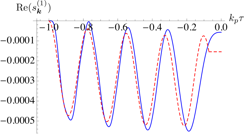
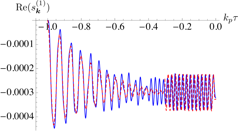
Figure 1: Time evolution of $\mathrm{Re}(s_{\boldsymbol{k}}^{(1)})$ in terms of normalized time $k_{p}\tau$. The KK mode is excited at $k_{p}\tau\approx-1$. Blue solid lines show numerically computed results, while the red dashed lines are the analytic estimations (5.17) - (5.19). Right (Left): Case for a wave mode that does (not) cross the resonance band.

One sees that the analytic estimations well describe the numerical results, except for at around the time $\tau_{\mathrm{res}}$ in the right figure, where we have made the simplifying assumption that the amplification happens instantaneously. It should be noted that parametric amplification actually happens roughly as $\propto(\tau-\tau_{\mathrm{res}})$, cf. (C.6).

We also note that in the analytic estimations, we have simply frozen the fluctuations at $\tau=-1/k$, which also give rise to errors for estimating the asymptotic values $\mathrm{Re}(s_{\boldsymbol{k}}^{(1)})|_{\tau\to 0^{-}}$. However, such errors only lead to shifts in the phase of the oscillations in the $\mathrm{Re}(s_{\boldsymbol{k}}^{(1)})$ spectrum in $k$-space, as we will see in the next subsection.

5.3 Curvature Perturbation Spectrum

The effects from the KK-mode oscillations on the curvature perturbation spectrum are captured by the asymptotic value $2\mathrm{Re}(s_{\boldsymbol{k}}^{(1)})|_{\tau\to 0^{-}}$, cf. (4.46). We obtain this analytically by freezing the expressions (5.17) and (5.19) at horizon exit $\tau=-1/k$.

For $k\leq-1/\tau_{\mathrm{exc}}$:

$$\mathrm{Re}(s_{\boldsymbol{k}}^{(1)})|_{\tau\to 0^{-}}\simeq 0.$$ (5.20)

For $-1/\tau_{\mathrm{exc}}\leq k\leq k_{n}$:

$$\mathrm{Re}(s_{\boldsymbol{k}}^{(1)})|_{\tau\to 0^{-}}\simeq\tilde{\eta}_{n\,\mathrm{exc}}\,\xi_{n\,\mathrm{exc}}\left[\left(2\cos 2\theta_{n}-\frac{1}{2}\right)\cos\left(2k\tau_{\mathrm{exc}}+2\right)-2\cos 2\theta_{n}-\frac{1}{2(k\tau_{\mathrm{exc}})^{3}}\right].$$ (5.21)

For $k_{n}\leq k$:

$$\mathrm{Re}(s_{\boldsymbol{k}}^{(1)})|_{\tau\to 0^{-}}\simeq 3^{3/2}\tilde{\eta}_{n\,\mathrm{exc}}\,\xi_{n\,\mathrm{exc}}^{1/2}\left(\frac{k_{n}}{k}\right)^{3}\cos\left\{\frac{4\cdot 3^{1/2}}{\xi_{n\,\mathrm{exc}}}\left(1+\ln\left(\frac{k}{k_{n}}\right)\right)-2+2\theta_{n}\right\}\\ +\tilde{\eta}_{n\,\mathrm{exc}}\,\xi_{n\,\mathrm{exc}}\left[\frac{1}{2}\left(\cos 2\theta_{n}-1\right)\cos\left(2k\tau_{\mathrm{exc}}+2\right)-2\cos 2\theta_{n}\right].$$ (5.22)

Here in (5.22) we have dropped a contribution originating from the term $(\tau/\tau_{\mathrm{exc}})^{3}$ in (5.19) which asymptotically becomes tiny. As stated in the previous subsection, the actual $\mathrm{Re}(s_{\boldsymbol{k}}^{(1)})$ spectrum is obtained by adding the above expressions over all excited KK-modes $n$.

The resonant peak rises at around $k=k_{n}$, dividing wave modes by whether or not they went through the resonance band. Here, since we have adopted the simplifying assumption of instantaneous resonant amplification, the above approximate expressions give a peak that rises suddenly at $k=k_{n}$. Actually, the resonant oscillations arise sharply but within a finite wave number range, reflecting the finite time interval that a wave mode stays in the resonance band. As is shown in the first term in (C.6), when in the resonance band, $s_{\boldsymbol{k}}^{(1)}$ is parametrically amplified roughly proportional to $(\tau-\tau_{\mathrm{res}})$. The rising region $\Delta k$ around $k_{n}$ consists of wave modes for which the KK excitation at $\tau_{\mathrm{exc}}$ happens to be within the range $\Delta\tau\sim-\xi_{n\,\mathrm{exc}}^{1/2}\tau_{\mathrm{res}}(k)$ (5.16) around their resonance times $\tau_{\mathrm{res}}(k)$. One can estimate that the resonant peak in the $k$-space rises sharply within a wave number interval of

$$\Delta k\sim\xi_{n\,\mathrm{exc}}^{1/2}k_{n},$$ (5.23)

around $k=k_{n}$. Thus actually the resonant oscillations peak at wave numbers slightly larger than $k_{n}$. One can also see that in the rising region (5.23), effects from parametric resonance (i.e. the first line of (5.22)) is dominant over other effects (i.e. second line of (5.22)).

In Figure 2 we illustrate a typical oscillation form induced on the curvature perturbation spectrum from an excited KK-mode with $\theta_{n}\approx 0$, i.e. $\dot{\psi}_{n\,\mathrm{exc}}\approx 0$. Wave modes that are sub-horizon at the KK excitation obtain oscillations about the offset $-2\tilde{\eta}_{n\,\mathrm{exc}}\,\xi_{n\,\mathrm{exc}}\cos 2\theta_{n}$. For modes in the range $-\tau_{\mathrm{exc}}^{-1}\leq k\lesssim k_{n}$ which do not cross the resonance band, the oscillation period is a constant $-\pi/\tau_{\mathrm{exc}}$, and the oscillation amplitude is comparable to the offset.

The oscillation amplitude obtains a peak of $\sim\tilde{\eta}_{n\,\mathrm{exc}}\xi_{n\,\mathrm{exc}}^{1/2}$ at the wave number $k\approx k_{n}$, beyond which the amplitude decays proportionally to $\propto k^{-3}$, with $k$-dependent oscillation period $-\pi/\tau_{\mathrm{res}}(k)\sim\xi_{n\,\mathrm{exc}}k$. Here one clearly sees that the induced oscillations are determined basically by the two parameters $\tilde{\eta}_{n\,\mathrm{exc}}$ and $\xi_{n\,\mathrm{exc}}$.

Let us further remark that for nonzero $\theta_{n}$, oscillations with period $-\pi/\tau_{\mathrm{exc}}$ is dominant also at wave numbers sufficiently larger than $k_{n}$, as can be seen from the second line of (5.22). (Such oscillations at large $k$ do exist even for $\theta_{n}=0$, though they are suppressed. See discussions below (5.19).) On the other hand, oscillations in the range $-\tau_{\mathrm{exc}}^{-1}\leq k\lesssim k_{n}$ are suppressed for $\cos 2\theta_{n}\approx 1/4$.

For smaller $\xi_{n\,\mathrm{exc}}$, i.e. heavier KK modes, the resonant peak rises more sharply, and thus the envelope of the oscillations takes a more asymmetric form in $k$-space.

Figure 2: Schematic of the oscillations on the curvature perturbation spectrum induced by an excited KK-mode with $\theta_{n}\approx 0$, i.e. $\dot{\psi}_{n\,\mathrm{exc}}\approx 0$. The envelope of the resonant oscillations is sharper and more asymmetric for smaller $\xi_{n\,\mathrm{exc}}$, i.e. for heavier KK modes.

We have also numerically computed the $\mathrm{Re}(s_{\boldsymbol{k}}^{(1)})$ spectrum as a function of the wave number, for the parameter set chosen in the previous subsection. The results are shown in Figure 3, where the blue solid lines show numerically calculated values of $\mathrm{Re}(s_{\boldsymbol{k}}^{(1)})$ at a time when all the displayed wave modes are well outside the horizon (and also when the KK mode has sufficiently damped away), and the red dashed lines denote the analytic estimations (5.20) - (5.22). One sees that the analytic result captures the overall behavior of the spectrum, though overestimates the resonant peak due to the approximation of the instantaneous parametric amplification. One can also see that as the dominant oscillation with period $-\pi/\tau_{\mathrm{res}}(k)$ decays away for large $k$, tiny oscillations with period $-\pi/\tau_{\mathrm{exc}}$ show up. Such oscillations are suppressed from $\theta_{1}=0$, but are present at sub-leading orders beyond the approximate estimation of (5.22).

Before ending this subsection, let us repeat that the particular forms of the oscillations generated by the KK modes can be attributed to a few parameters, which are $\tilde{\eta}_{n\,\mathrm{exc}}$ representing the excited KK amplitudes, and $\xi_{n\,\mathrm{exc}}$ setting the effective masses of the KK modes. In addition to these two parameters, the time of KK excitation $\tau_{\mathrm{exc}}$ determines where in $k$-space the oscillations rise.

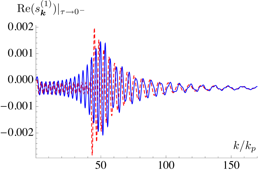
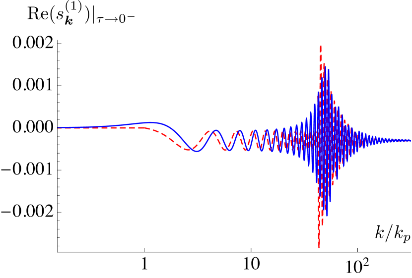
Figure 3: Asymptotic values of $\mathrm{Re}(s_{\boldsymbol{k}}^{(1)})$, denoting the KK induced oscillations on the curvature perturbation spectrum $\frac{1}{2}(\mathcal{P}_{\zeta}(k)/\mathcal{P}_{\zeta 0}(k)-1)$, as a function of wave number in linear (left figure) and log (right) scales. Blue solid lines show numerically computed results, while the red dashed lines are the analytic estimations (5.20) - (5.22).

5.4 Effects from Multiple KK Modes

As we have stated above, for small KK excitations, effects from multiple KK modes simply add up. As an example, in Figure 4 we show the numerically computed $\mathrm{Re}(s_{\boldsymbol{k}}^{(1)})$ spectrum for the case where two KK modes $n=1$, $2$ are excited. The parameters are the same as in the previous subsections, except for that the $n=2$ mode is further excited with $\alpha_{2}=200$, $\tilde{\psi}_{2\,\mathrm{exc}}=0.0004M_{p}$, $\theta_{2}=0$. (Note that $\alpha_{n}\propto n$, $\xi_{n\,\mathrm{exc}}\propto n^{-1}$, $\tilde{\eta}_{n\,\mathrm{exc}}\propto n^{3}\tilde{\psi}_{n\,\mathrm{exc}}^{2}$, and $k_{n}\propto n$.) The plot shows superimposed oscillations from the two KK modes, which are peaked at around $k_{1}\approx 42k_{p}$ and $k_{2}\approx 85k_{p}$.

Let us also note that effects from multiple KK modes can cancel each other, given that the excited KK amplitudes obey specific hierarchies such that different $n$ modes produce $\mathrm{Re}(s_{\boldsymbol{k}}^{(1)})$ with similar oscillation amplitudes/offsets, and further if the phases $\theta_{n}$ take appropriate values. When focusing on a certain wave number $k$ and considering the time evolution of $\mathrm{Re}(s_{\boldsymbol{k}}^{(1)})$, its oscillation amplitude can be suppressed (instead of amplified) when going through multiple resonance bands, if the phases $\theta_{n}$ of the KK modes are suitably distributed, cf. first line of (5.19). However, the resonant oscillations of the $\mathrm{Re}(s_{\boldsymbol{k}}^{(1)})$ spectrum in $k$-space (i.e. first line of (5.22)) cannot be cancelled entirely, since $\xi_{n\,\mathrm{exc}}\propto n^{-1}$ and thus different $n$ modes source different oscillation periods.

As we have seen explicitly, the KK tower generates oscillations on the curvature perturbation spectrum with specific patterns characterized by the integers $n$. It would be very interesting to investigate such specific patterns in cosmological observables, which can allow us to extract information about the extra dimensional space.

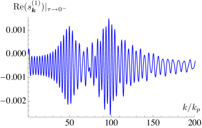
Figure 4: $\mathrm{Re}(s_{\boldsymbol{k}}^{(1)})$ spectrum in $k$-space when two KK modes are excited.

6 Strong Resonance from Large KK Excitations

In this section we study cases with large KK excitations beyond the condition (3.20), i.e., when (3.7) - (3.10) are no longer good approximations of the inflationary dynamics. We will see that when the KK mode amplitudes are as large as $\tilde{\eta}_{n\,\mathrm{exc}}\xi_{n\,\mathrm{exc}}\gtrsim 0.1$, the inflaton field fluctuations are strongly amplified through parametric resonance, generating sharp spikes in the curvature perturbation spectrum.

6.1 Curvature Perturbation Spectrum

Let us first show how the resulting curvature perturbation spectrum changes when the KK mode is excited with larger amplitude. In Figures 5, 6, and 7, we show the results for the case where the $n=1$ KK mode is excited at about 50 e-foldings before the end of inflation. The parameters are chosen similarly as in the previous section, i.e. $\phi_{\mathrm{exc}}\approx 8.2M_{p}$, $\mu\approx 0.0016M_{p}$, $\alpha_{1}=100$, but with various KK mode amplitudes $\psi_{1\,\mathrm{exc}}$. We again use $k_{p}$ to denote the wave number that exits the horizon at around the time of KK excitation. (The following parameters are also the same as in the previous section: $\epsilon_{\mathrm{exc}}\approx 0.015$, $\xi_{1\,\mathrm{exc}}\approx 0.082$, and $k_{1}\approx 42k_{p}$, though $k_{1}$ defined in (5.14) no longer denotes the position of the resonant peak for strong resonance.) The excited KK mode amplitudes are taken as $\tilde{\psi}_{1\,\mathrm{exc}}=0.001M_{p}$ ($\tilde{\eta}_{1\,\mathrm{exc}}\approx 0.0018$), $\tilde{\psi}_{1\,\mathrm{exc}}=0.01M_{p}$ ($\tilde{\eta}_{1\,\mathrm{exc}}\approx 0.18$), and $\tilde{\psi}_{1\,\mathrm{exc}}\approx 0.033M_{p}$ ($\tilde{\eta}_{1\,\mathrm{exc}}\approx 2.0$), respectively, for Figures 5, 6, and 7, with vanishing initial velocity $\dot{\psi}_{1\,\mathrm{exc}}=0$. Upon obtaining the power spectrum, we have numerically solved the full set of equations of motion for the homogeneous background (3.2), (3.4), and (3.6), as well as for the inflaton field fluctuation $q_{\boldsymbol{k}}$ (4.5). Note that even when the KK modes are largely excited, the power spectrum can be obtained by evaluating (4.43) when the wave modes have exited the horizon (4.41) and the KK mode oscillations are damped away such that $\eta_{n}$ is sufficiently smaller than unity, satisfying for e.g. (4.42). This gives the power spectrum within errors of $\mathcal{O}(\epsilon,\eta_{n})$ upon evaluation. We have assumed the KK mode to be excited suddenly to $\tilde{\psi}_{n\,\mathrm{exc}}$, which sources unphysical jumps at $t_{\mathrm{exc}}$ in quantities such as the Hubble parameter. However, we expect this treatment to be valid for discussing the KK signals since it is the parametric resonance following the KK excitation that sources sharp features in the perturbation spectrum.

In the figures on the left side, the blue solid lines denote the power spectrum $\mathcal{P}_{\zeta}$ of the curvature perturbations, shown with log scale for the wave number. The black dot-dashed lines represent the spectrum $\mathcal{P}_{\zeta 0}$ in the absence of the KK mode. On the right side, we show in blue solid lines the ratio $(\mathcal{P}_{\zeta}-\mathcal{P}_{\zeta 0})/\mathcal{P}_{\zeta 0}$ denoting the relative amplitude of the KK mode effects, with linear scale for the wave number. For comparison, we have also plotted the red dashed lines which are the asymptotic values of $2\mathrm{Re}(s_{\boldsymbol{k}}^{(1)})$, obtained by solving (4.33), with (4.25), (4.30), and (4.31). As we have discussed in the previous section, $2\mathrm{Re}(s_{\boldsymbol{k}}^{(1)})$ represents $(\mathcal{P}_{\zeta}-\mathcal{P}_{\zeta 0})/\mathcal{P}_{\zeta 0}$ in the small KK regime $\tilde{\eta}_{n\,\mathrm{exc}}\ll 1$ (cf. (4.46)), as is seen in Figure 5. However, $2\mathrm{Re}(s_{\boldsymbol{k}}^{(1)})$ fails in describing the KK effects as $\tilde{\eta}_{n\,\mathrm{exc}}$ increases and the small KK approximations break down. As the KK amplitude increases, the resonant oscillations around $k=k_{1}$ grow asymmetrically towards the positive side of $\mathcal{P}_{\zeta 0}$, and eventually form sharp spikes on the power spectrum.

The strong parametric resonance significantly enhances the inflaton field fluctuations, and the resulting spikes in the perturbation spectrum grows non-linearly with respect to $\tilde{\eta}_{n\,\mathrm{exc}}$. A slight increase in the KK amplitude enhances the spike by orders of magnitude, for e.g., $\tilde{\psi}_{n\,\mathrm{exc}}=0.05M_{p}$ sources $(\mathcal{P}_{\zeta}-\mathcal{P}_{\zeta 0})/\mathcal{P}_{\zeta 0}$ as large as $\sim 3000$ at its peak. It should also be noted that the peak of the oscillations/spikes is shifted slightly towards larger $k$ for strong parametric resonance, as can be seen in Figure 7. While the amplitude of the oscillations on $\mathcal{P}_{\zeta}$ are significantly enhanced by the strong resonance, the oscillation period follows similar behavior as for the weak resonance. Moreover, the oscillations at wave numbers away from the peak (e.g. $k\lesssim 40k_{p}$ and $k\gtrsim 70k_{p}$ in Figure 7) are not so different from the weak resonant calculations represented by $2\mathrm{Re}(s_{\boldsymbol{k}}^{(1)})$. Here we also remark that when the resonance is very strong, the spectrum can obtain multiple peaks, although the one at the wave number slightly larger than $k_{1}$ is the largest.

The resonant spikes grow significantly as the KK amplitude is increased, until $\tilde{\psi}_{n\,\mathrm{exc}}$ becomes so large that the field dynamics are completely modified and/or the higher order KK interactions are important. For the Lagrangian (2.13) with the set of parameters chosen here, the KK mode no longer oscillates when $\tilde{\psi}_{n\,\mathrm{exc}}\gtrsim 0.06$ (or $\tilde{\eta}_{n\,\mathrm{exc}}\gtrsim 6$). In addition, $B_{\phi\phi}$ becomes negative and thus the inflaton field fluctuation $q$ is tachyonic, cf. (4.3). However we should remark that in such case the product of $\tilde{\eta}_{n\,\mathrm{exc}}$ and $\xi_{n\,\mathrm{exc}}$ is as large as $\tilde{\eta}_{n\,\mathrm{exc}}\xi_{n\,\mathrm{exc}}\gtrsim 0.5$ and the condition (3.24) is almost broken. Hence the cubic or higher order KK terms in the Lagrangian can become important, and may prevent $q$ from becoming tachyonic. It would be very interesting to explore this regime, where the higher order KK terms may contribute to source even stronger resonant features in the primordial spectrum.

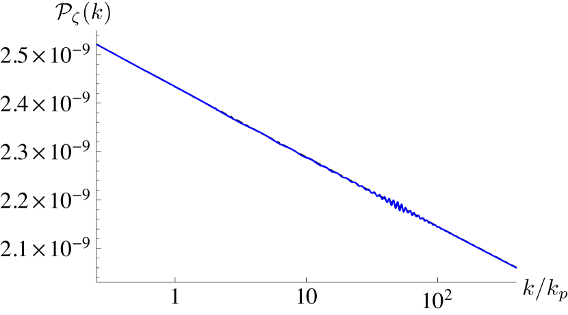
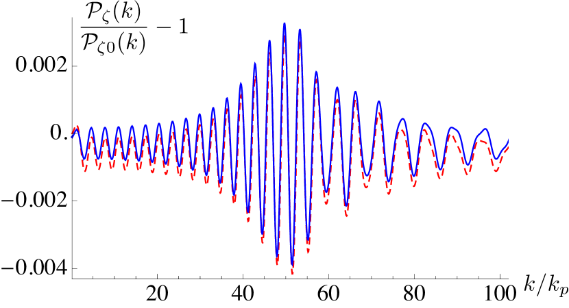
Figure 5: Curvature perturbation spectrum with KK mode $\tilde{\psi}_{1\,\mathrm{exc}}=0.001M_{p}$ ($\tilde{\eta}_{1\,\mathrm{exc}}\approx 0.0018$).

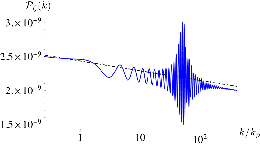
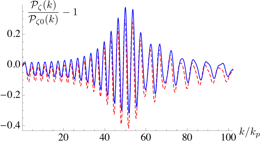
Figure 6: Curvature perturbation spectrum with KK mode $\tilde{\psi}_{1\,\mathrm{exc}}=0.01M_{p}$ ($\tilde{\eta}_{1\,\mathrm{exc}}\approx 0.18$).

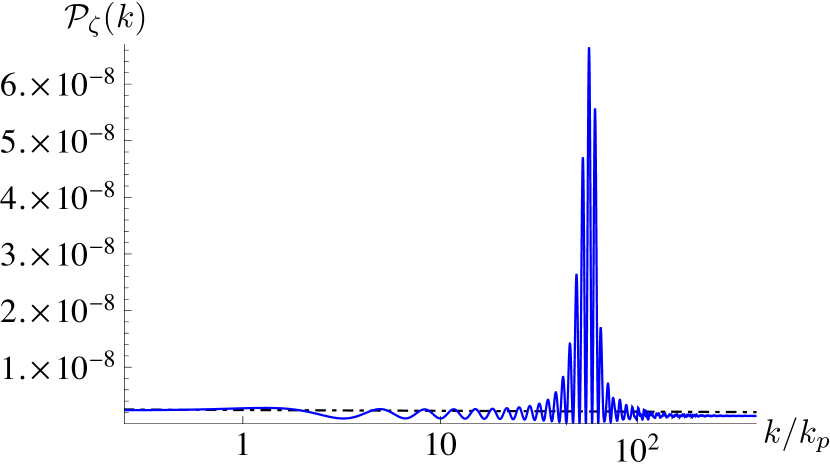
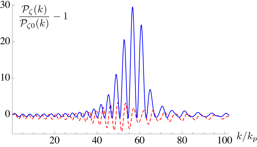
Figure 7: Curvature perturbation spectrum with KK mode $\tilde{\psi}_{1\,\mathrm{exc}}\approx 0.033M_{p}$ ($\tilde{\eta}_{1\,\mathrm{exc}}\approx 2.0$).

6.2 Effective Frequency

The behavior of the strong resonance can be better understood by studying how the oscillation frequency of $q_{\boldsymbol{k}}$ resonates with that of the KK modes. For this purpose, let us redefine the field fluctuation as

$$u_{\boldsymbol{k}}\equiv(aB_{\phi\phi})^{1/2}q_{\boldsymbol{k}},$$ (6.3)

so that its equation of motion takes the form

$$0=\ddot{u_{\boldsymbol{k}}}+f_{k\,\mathrm{eff}}^{2}\,u_{\boldsymbol{k}},$$ (6.4)

where $f_{k\,\mathrm{eff}}^{2}$ denotes the effective frequency squared defined as

$$f_{k\,\mathrm{eff}}^{2}(t)\equiv\frac{2L_{A}G^{A}_{\phi\phi}}{B_{\phi\phi}}\frac{k^{2}}{a^{2}}-\frac{M_{\phi\phi}}{B_{\phi\phi}}+\frac{\left(a^{3}C_{\phi\phi}\right)^{\cdot}}{a^{3}B_{\phi\phi}}-\frac{\left(a^{3/2}B_{\phi\phi}^{1/2}\right)^{\cdot\cdot}}{a^{3/2}B_{\phi\phi}^{1/2}}.$$ (6.5)

The oscillating KK modes force the frequency $f_{k\,\mathrm{eff}}^{2}$ itself to oscillate in time, and when $f_{k\,\mathrm{eff}}^{2}$ becomes similar to the KK mode frequency $\sim m_{\mathrm{KK}}$, the field fluctuation $u_{\boldsymbol{k}}$ experiences parametric resonance. The weak resonance discussed in Section 5 corresponds to tiny oscillations of $f_{k\,\mathrm{eff}}^{2}$, and the strong resonance happens when $f_{k\,\mathrm{eff}}^{2}$ oscillates considerably.

In Figure 8 we plot the time evolution of the field fluctuation $u_{\boldsymbol{k}}$ and its effective frequency $f_{k\,\mathrm{eff}}^{2}$ for the case of $\tilde{\psi}_{1\,\mathrm{exc}}\approx 0.033M_{p}$ and $k\approx 57k_{p}$. This wave number is where the resonant spike is peaked at in Figure 7. The time is shown in units of the KK mode oscillation period $2\pi/m_{\mathrm{KK}}\simeq\pi\phi_{\mathrm{exc}}/\alpha_{1}V_{\mathrm{exc}}^{1/2}$, therefore is equivalent to the number of oscillations of $\psi_{1}$. Here, recall that the KK modes affect $f_{k\,\mathrm{eff}}^{2}$ through quadratic terms (see e.g. (4.6)), hence $f_{k\,\mathrm{eff}}^{2}$ oscillates with half the period of the KK mode. The KK mode is excited at $t=0$ in the figures. In the left figure we show the growth of the fluctuation $|u_{\boldsymbol{k}}|$ relative to its value at the KK excitation $|u_{\boldsymbol{k}\,\mathrm{exc}}|$. In the right figure, the blue solid line denotes the ratio $f_{k\,\mathrm{eff}}^{2}/m_{\mathrm{KK}}^{2}$ between the effective frequency of $u_{\boldsymbol{k}}$ and the KK mass. Moreover, the red dashed line shows $k^{2}/a^{2}m_{\mathrm{KK}}^{2}$, while the black dot-dashed line at unity represents the KK mass squared. We remark that the displayed wave mode $k\approx 57k_{p}$ is inside the horizon in the plotted time range.

In the absence of the KK modes, the effective frequency $f_{k\,\mathrm{eff}}^{2}$ traces $k^{2}/a^{2}$ when the wave mode is inside the horizon. This is still the case for small KK excitations triggering weak resonance discussed in Section 5. However when the KK modes are largely excited, $f_{k\,\mathrm{eff}}^{2}$ considerably oscillates and can even become negative. From the figures, one sees that $u_{\boldsymbol{k}}$ is enhanced by an order of magnitude soon after the KK mode excitation, while $f_{k\,\mathrm{eff}}^{2}$ wildly oscillates around $m_{\mathrm{KK}}^{2}$. The fluctuation $u_{\boldsymbol{k}}$ initially oscillates with twice the frequency of the KK mode (i.e. the period matches with the tics on the time axis), and is enhanced at each oscillation. As $f_{k\,\mathrm{eff}}^{2}$ becomes smaller than $m_{\mathrm{KK}}^{2}$, parametric resonance ceases and $|u_{\boldsymbol{k}}|$ starts to increase slowly in time as $\propto\sim a^{1/2}$. (Note that, in the absence of the KK modes, $|u_{\boldsymbol{k}}|$ scales proportional to $a^{1/2}$ when inside the horizon, and as $a^{3/2}$ after horizon exit, as can be seen from its definition (6.3) and (4.24).) Let us also remark that the parametric resonance of the inflaton field fluctuation shares common features with preheating [38, 39]. We have studied that parametric resonance happens for $u_{\boldsymbol{k}}$ when its effective frequency $f_{k\,\mathrm{eff}}^{2}$ oscillates with frequency similar to itself, hence in this sense, both the weak and strong resonance is analogous to the narrow resonance in preheating.

In Figures 5 - 7 we have seen that the resonant peak in the perturbation spectrum slightly shift towards larger $k$ for stronger resonance. This can be understood from the oscillating $f_{k\,\mathrm{eff}}^{2}$ mostly taking values that are smaller than $k^{2}/a^{2}$. In other words, the characteristic frequency of $u_{\boldsymbol{k}}$ effectively becomes smaller than $k/a$, and therefore the resonant features shift towards (slightly) larger wave numbers.

The oscillations of the effective frequency $f_{k\,\mathrm{eff}}^{2}$ are quickly suppressed as the KK mode oscillations damp away. The wave modes that enter the resonance band while the oscillations are large experience strong parametric resonance, and moreover, such resonant effects depend non-linearly on the KK amplitude (squared). This is why the strong enhancement of the curvature perturbations can be localized to a narrow wave number range, forming spikes in the perturbation spectrum.

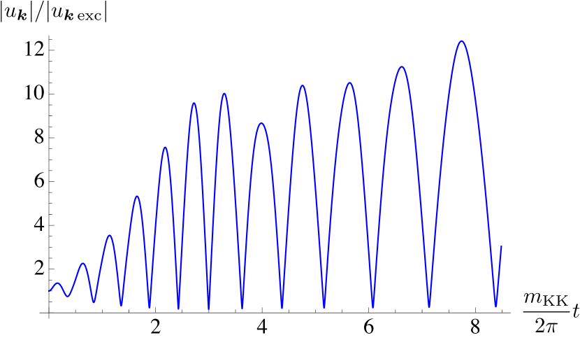
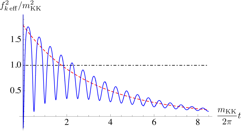
Figure 8: Time evolution of the inflaton field fluctuation $u_{\boldsymbol{k}}$ (left figure) and its effective frequency squared (right figure), for $\tilde{\psi}_{1\,\mathrm{exc}}\approx 0.033M_{p}$ and $k\approx 57k_{p}$. The time is shown in units of the oscillation period of the KK mode $2\pi/m_{\mathrm{KK}}$, and the KK mode is excited at $t=0$.

6.3 Condition for Strong Resonance

For the set of parameters chosen in Section 6.1, the oscillation of the effective frequency $f_{k\,\mathrm{eff}}^{2}$ (6.5) is dominated by its components

$$\frac{2L_{A}G^{A}_{\phi\phi}}{B_{\phi\phi}}\frac{k^{2}}{a^{2}}+\frac{1}{4}\left(\frac{\dot{B_{\phi\phi}}}{B_{\phi\phi}}\right)^{2}-\frac{1}{2}\frac{\ddot{B_{\phi\phi}}}{B_{\phi\phi}},$$ (6.6)

and furthermore, by the same terms that were important for weak resonance, i.e., the terms explicitly written in (4.6), (4.7), and (4.8). Recall that these terms originate from the three kinetic couplings (4.14) in the inflaton Lagrangian. Here we focus on those terms and quantitatively discuss the strong parametric resonance. We note that our aim here is to give a rough estimate on when strong resonance happens, and in this subsection we use some identities without proof.

As a rule of thumb, we consider strong resonance to happen for wave modes in the resonance band if $f_{k\,\mathrm{eff}}^{2}$ oscillates with amplitude as large as $k^{2}/a^{2}$. This happens if, for e.g., $B_{\phi\phi}$ in the denominator of the first term in (6.6) oscillates substantially. Using $\psi_{n}\simeq\tilde{\psi}_{n}\cos(2\alpha_{n}V^{1/2}t/\phi+\cdots)$ and $\dot{\psi}_{n}\simeq-2\alpha_{n}V^{1/2}\tilde{\psi}_{n}\sin(2\alpha_{n}V^{1/2}t/\phi+\cdots)$, then one finds from (4.6) that $B_{\phi\phi}$ oscillates with amplitude of order unity or larger for (for simplicity we consider a single KK mode excitation),

$$0.1\lesssim\alpha_{n}^{2}\frac{\tilde{\psi}_{n\,\mathrm{exc}}^{2}}{\phi_{\mathrm{exc}}^{2}}=\tilde{\eta}_{n\,\mathrm{exc}}\xi_{n\,\mathrm{exc}}.$$ (6.7)

One can further check that the other terms in (6.6) also oscillate $f_{k\,\mathrm{eff}}^{2}$ with amplitude $\sim k^{2}/a^{2}$ for similar KK amplitudes while in the resonance band. Therefore, we can consider (6.7) as the rough indicator for strong resonance to happen.

A wave mode undergoes strong resonance if it approaches the resonance band (i.e. $k^{2}/a^{2}\sim m_{\mathrm{KK}}^{2}$) while (6.7) holds. Denoting the largest (smallest) wave number that experiences strong resonance by $k_{\mathrm{max}}$ ($k_{\mathrm{min}}$), then from $\tilde{\eta}_{n}\xi_{n}\propto\sim a^{-3}$ one can estimate the ratio

$$\frac{k_{\mathrm{max}}}{k_{\mathrm{min}}}\sim\left(10\tilde{\eta}_{n\,\mathrm{exc}}\xi_{n\,\mathrm{exc}}\right)^{1/3}.$$ (6.8)

Therefore, in the regime (3.24) where one can neglect the cubic or higher order KK terms in the Lagrangian, the wave interval over which strongly resonant features arise is quite narrow. Moreover, since the strong resonant amplification non-linearly depends on the KK amplitudes, the resonant features can further have hierarchical structures.

7 Conclusions

Wrapped brane inflation necessarily possesses infinite KK degrees of freedom in addition to the zero-mode inflaton, and the brane’s Nambu-Goto action naturally gives kinetic couplings among them. In this paper, we have investigated resonant amplification of the curvature perturbations triggered by the KK oscillations during inflation. We found that the resonant signals in the perturbation spectrum can be localized to narrow wave number ranges, in contrast to previous studies where signals were normally distributed over a rather wide $k$-range. In the effective four dimensional theory, the zero-mode inflaton couples to the heavy KK modes which are excited and oscillates during inflation. Small KK excitations lead to weak resonance, sourcing oscillatory features in the perturbation spectrum (cf. Figure 2, 5) whose oscillation amplitude is proportional to the excited KK amplitude squared. For larger KK excitations, the resonant amplification becomes extremely efficient with non-linear dependence on the KK amplitude. We saw that such strong resonant effects damp more rapidly than the KK oscillations during inflation, therefore leave spiky features localized to a narrow wave number range in the perturbation spectrum (cf. Figure 7). Both weak and strong resonant effects were mainly sourced by the couplings between the inflaton kinetic terms and the oscillating KK modes.

Motivated by the string theory construction of [6], we have supposed the brane tension to be the main driving force for inflation and considered only the Nambu-Goto action. However we note that, even if there are further contributions to the brane potential, the Nambu-Goto action gives the kinetic terms that contain the important interactions with the KK modes. Therefore we expect the resonant effects studied in this paper to be rather generic features for inflation driven by extended sources. From an effective theory point of view, it would also be interesting to systematically examine resonant effects arising from kinetic couplings in general.

We have restricted ourselves to KK modes that are not excited too largely and thus studied up to quadratic KK interactions in the Lagrangian. Some region of the strong resonance was close to the regime where the higher order KK terms can become important, thus it is of interest to analyze effects from higher order interactions. Especially when going beyond the strong resonance regime we have studied, the tower of KK interactions may further enhance the resonant signals.

The wrapped brane model provides an example where the kinetic couplings between the inflaton and the heavy KK modes produce sharp features in the curvature perturbation spectrum, and to that end we have focused on the evolution of the perturbations under the KK oscillations. Although the KK modes can be excited as the wrapped inflaton brane passes by structures or localized sources along the inflationary trajectory, we have not yet specified the excitation mechanism in detail. It would be very interesting to study the whole picture including dynamical excitation of the KK modes. One can imagine that the KK excitation is triggered as the inflaton comes across some point(s) in field space. Then the KK excitation itself may become inhomogeneous and give further contributions to the curvature perturbations. It could also be that the KK modes are repeatedly excited during inflation, if, for example, the trajectory of the wrapped brane is a repeated circuit as in monodromy models [6, 7]. In such case, the spikes/oscillations would repeatedly show up in the perturbation spectrum with the interval corresponding to the size of the inflaton circuit. Let us further mention that, if the KK excitations are triggered by another brane along the inflationary trajectory in string theory models, then as the branes encounter each other, strings stretched between them can become massless and be produced [41]. Such effects can slow down the inflaton brane, and may further generate oscillations/bumps in the perturbation spectrum by temporarily affecting the inflaton dynamics, and also by the produced strings (or particles in the effective theory) rescattering off the inflaton condensate, see e.g. [42, 43, 44, 45]. However, these signals are present for wide ranges of the wave number, thus can be distinguished from the sharp spikes sourced by the KK oscillations. We also note that, when constructing explicit models for wrapped brane inflation, the fate of the excited KK modes need to be taken into account, especially in relation to the moduli problem [46, 47, 48]. (See also [49] for discussions in this direction.)

Interestingly, the resonant signals in the curvature perturbations are characterized by the microphysics of the KK modes, which is tied to the properties of the internal manifold. The height of the spikes/oscillations are basically determined by the excited amplitude of the KK modes, while the width and oscillation period of the features in $k$-space are set by the KK mass corresponding to the size of the wrapped cycle. The positions of the resonant signals in $k$-space tell us when during inflation the KK modes were excited (possibly denoting the positions of localized sources in the internal manifold), and furthermore, the KK tower generates signals periodic in wave number $k$, cf. Figure 4. All these features open up possibilities for probing the extra dimensional space through cosmological experiments. It will also be interesting to study how well we may detect and measure these resonant signals through observations of the cosmic microwave background (CMB) and large scale structure. The oscillatory features from weak resonance may be somewhat smoothed out by the CMB transfer function (as is discussed in, e.g. [25]), but the spikes from strong resonance are expected to leave distinct imprints in the CMB temperature anisotropy. We leave to future work a detailed analysis of the observational consequences of weak/strong resonance during inflation. We should also mention that the resonant signals can show up in the non-Gaussian signals as well, as discussed in [16, 17, 23]. It is quite possible that the strong resonance which sources spikes in the power spectrum also leave violent marks on the higher order correlation functions.

Appendix A Primordial Density Perturbations from Multi-Field Inflation with Various Kinetic Terms

In this appendix we consider density perturbations from multi-field inflation with an action containing various forms of kinetic terms. We make use of the $\delta\mathcal{N}$-formalism [33, 34, 35, 36] for obtaining the density perturbations, so here we simply derive the action of the field fluctuations up to quadratic order. The calculations are an extension of the previous works discussing inflationary models with multi-fields and/or non-canonical kinetic terms, e.g. [50, 51, 52, 53, 54]. We also refer the reader to [55, 56] which discuss similar Lagrangians as in this appendix.

The action we consider is of the following form:

$$S=\int d^{4}x\sqrt{-g}\left\{\frac{M_{p}^{2}}{2}R+L\left(\varphi^{I},\,X^{A}\right)\right\},$$ (A.1)

where $\varphi^{I}$ denotes the fields (labeled by $I$), and $X^{A}$ the kinetic terms,

$$X^{A}\equiv-G^{A}_{IJ}g^{\mu\nu}\partial_{\mu}\varphi^{I}\partial_{\nu}\varphi^{J}.$$ (A.2)

$G^{A}_{IJ}$ is the field space metric, where $A$ labels different metrics, i.e. different forms of kinetic terms. We impose $G^{A}_{IJ}=G^{A}_{JI}$, and consider $G^{A}_{IJ}$ to be constants (in other words, independent of $\varphi^{I}$). Note that in this appendix we label fields by $I,J,\cdots$, and field metrics by $A,B,\cdots$. Moreover, we express partial derivatives in terms of $\varphi^{I}$ and $X^{A}$ as, respectively,

$$L_{I}\equiv\frac{\partial L}{\partial\varphi^{I}},\quad L_{A}\equiv\frac{\partial L}{\partial X^{A}}.$$ (A.3)

Then one can derive the energy-momentum tensor,

$$T_{\mu\nu}=g_{\mu\nu}L-2\frac{\partial L}{\partial g^{\mu\nu}}=g_{\mu\nu}L+2L_{A}G^{A}_{IJ}\partial_{\mu}\varphi^{I}\partial_{\nu}\varphi^{J},$$ (A.4)

as well as the equation of motion of $\varphi^{I}$,

$$L_{I}+\frac{2}{\sqrt{-g}}\partial_{\mu}\left(\sqrt{-g}L_{A}G^{A}_{IJ}g^{\mu\nu}\partial_{\nu}\varphi^{J}\right)=0.$$ (A.5)

A.1 Homogeneous Background

First let us derive the equations of motion of the homogeneous background. We fix the background metric to a flat FRW:

$$ds^{2}=-dt^{2}+a^{2}(t)\delta_{ij}dx^{i}dx^{j},$$ (A.6)

where $i,j=1,2,3$ run over the spatial directions.

Then the Einstein equations are

$$3M_{p}^{2}H^{2}=-L+2L_{A}G^{A}_{IJ}\dot{\varphi}^{I}\dot{\varphi}^{J},$$ (A.7)

$$-M_{p}^{2}(2\dot{H}+3H^{2})=L,$$ (A.8)

where an overdot denotes a time derivative, and $H=\dot{a}/a$.

The equation of motion of $\varphi^{I}$ (A.5) now takes the form

$$L_{I}-2\left(L_{A}G^{A}_{IJ}\dot{\varphi}^{J}\right)^{\cdot}-6HL_{A}G^{A}_{IJ}\dot{\varphi}^{J}=0.$$ (A.9)

A.2 Field Fluctuations

We then study fluctuations around the homogeneous background. We adopt the ADM formalism,

$$ds^{2}=-N^{2}dt^{2}+h_{ij}(dx^{i}+N^{i}dt)(dx^{j}+N^{j}dt),$$ (A.10)

under which the action (A.1) is rewritten as (we take $N>0$):

$$S=\int dtd^{3}xN\sqrt{h}\left[\frac{M_{p}^{2}}{2}\left\{R^{(3)}+\frac{1}{N^{2}}\left(E_{ij}E^{ij}-E^{2}\right)\right\}+L\right].$$ (A.11)

Here $h\equiv\det(h_{ij})$, and $R^{(3)}$ is the scalar curvature on the $t=\mathrm{const.}$ spatial hypersurface. The symmetric tensor $E_{ij}$ is defined as

$$E_{ij}\equiv\frac{1}{2}\left(\dot{h}_{ij}-\nabla_{i}N_{j}-\nabla_{j}N_{i}\right),$$ (A.12)

where $\nabla_{i}$ is a derivative associated with $h_{ij}$, and $E=h^{ij}E_{ij}$. We also note that the indices $i,j$ are raised and lowered by $h^{ij}$ and $h_{ij}$, respectively. $X^{A}$ is now expressed as

$$X^{A}=-G^{A}_{IJ}\left\{-\frac{1}{N^{2}}\dot{\varphi}^{I}\dot{\varphi}^{J}+\left(h^{ij}-\frac{N^{i}N^{j}}{N^{2}}\right)\partial_{i}\varphi^{I}\partial_{j}\varphi^{J}+2\frac{N^{i}}{N^{2}}\dot{\varphi}^{I}\partial_{i}\varphi^{J}\right\}.$$ (A.13)

Hereafter we take uniform curvature slicing, such that $t=\mathrm{const.}$ slices have vanishing Ricci curvature, thus

$$h_{ij}=a(t)^{2}\delta{ij},\qquad R^{(3)}=0,\qquad\nabla_{i}\to\partial_{i},$$ (A.14)

and the action becomes

$$S=\int dtd^{3}x\sqrt{h}\left[\frac{M_{p}^{2}}{2N}\left(E_{ij}E^{ij}-E^{2}\right)+NL\right].$$ (A.15)

We will focus on the field fluctuations $Q^{I}$ defined as

$$\varphi^{I}=\varphi^{I}_{0}+Q^{I}$$ (A.16)

where $\varphi_{0}^{I}$ is the homogeneous classical background, and later on convert them into the curvature perturbations using the $\delta\mathcal{N}$-formalism (A.36).

The lapse $N$ and shift $N^{i}$ are Lagrange multipliers in the action (A.15), hence their equations of motion can be used as constraints, which are, respectively,

$$N^{2}L=\frac{M_{p}^{2}}{2}\left(E_{ij}E^{ij}-E^{2}\right)+2L_{A}G^{A}_{IJ}v^{I}v^{J},$$ (A.17)

$$M_{p}^{2}\partial_{j}\left\{\frac{1}{N}\left(E^{ij}-Eh^{ij}\right)\right\}=\frac{2}{N}L_{A}h^{ij}G^{A}_{IJ}v^{I}\partial_{j}\varphi^{J}.$$ (A.18)

Here we have defined

$$v^{I}\equiv\dot{\varphi}^{I}-N^{i}\partial_{i}\varphi^{I}.$$ (A.19)

Let us rewrite the lapse and shift as

$$\begin{split}N&=1+\alpha,\\ N_{i}&=\partial_{i}\psi+\widetilde{N}_{i},\end{split}$$ (A.20)

where $\widetilde{N}_{i}$ is the incompressible part, i.e.,

$$h^{ij}\partial_{j}\widetilde{N}_{i}=0.$$ (A.21)

We further expand the functions in terms of the field fluctuations $Q$,

$$\begin{split}\alpha&=\alpha_{1}+\alpha_{2}+\cdots,\\ \psi&=\psi_{1}+\psi_{2}+\cdots,\\ \widetilde{N}_{i}&=\widetilde{N}_{i}^{(1)}+\widetilde{N}_{i}^{(2)}+\cdots,\end{split}$$ (A.22)

where the numbers represent orders of $Q$, e.g. $\alpha_{n}=\mathcal{O}(Q^{n})$. We require the constraint equations to hold order by order.

In order to expand the action up to second order in $Q$, one needs to consider the lapse and shift only up to the first order, i.e. $\alpha_{1}$, $\psi_{1}$, and $\widetilde{N}_{i}^{(1)}$ (cf. [50, 53]). The constraint equation (A.17) at its zeroth order reproduce the Friedmann equation (A.7), while its first order is

$$\frac{2M_{p}^{2}H}{a^{2}}\delta^{ij}\partial_{i}\partial_{j}\psi_{1}=L_{I}^{(0)}Q^{I}+L_{A}^{(0)}G^{A}_{IJ}\left(-2\alpha_{1}\dot{\varphi}_{0}^{I}\dot{\varphi}_{0}^{J}+2\dot{\varphi}_{0}^{I}\dot{Q}^{J}\right)+2\alpha_{1}L^{(0)}\\ -4L_{A}^{(0)}G^{A}_{IJ}\dot{Q}^{I}\dot{\varphi}_{0}^{J}-2\left(L_{AI}^{(0)}Q^{I}+L_{AB}^{(0)}X_{1}^{B}\right)G^{A}_{IJ}\dot{\varphi}_{0}^{I}\dot{\varphi}_{0}^{J},$$ (A.23)

where we have used (A.7) upon obtaining this form. The zeroth order of (A.18) is trivial, and the first order is

$$2\partial_{i}\left(M_{p}^{2}H\alpha_{1}-L_{A}^{(0)}G^{A}_{IJ}\dot{\varphi}^{I}_{0}Q^{J}\right)=\frac{M_{p}^{2}}{2}h^{jk}\partial_{j}\partial_{k}\widetilde{N}_{i}^{(1)}.$$ (A.24)

Since $h^{ij}\partial_{i}(h^{kl}\partial_{k}\partial_{l}\widetilde{N}_{j}^{(1)})=0$, after choosing proper boundary conditions, one arrives at

$$h^{ij}\partial_{i}\partial_{j}\widetilde{N}_{k}^{(1)}=0,$$ (A.25)

$$M_{p}^{2}H\alpha_{1}=L_{A}^{(0)}G^{A}_{IJ}\dot{\varphi}_{0}^{I}Q^{J}.$$ (A.26)

We also note that the evolution equation (A.8) is obtained by combining the zeroth order of (A.17) (i.e. the Friedmann equation) and the zeroth order equation of motion of $\varphi^{I}$.

Using the zeroth order of (A.17), the zeroth order equation of motion of $\varphi^{I}$, and the first order of (A.18) (i.e. (A.25) and (A.26)), one can expand the action up to second order in $Q$,

$$\begin{split}S\triangleq\int d^{3}xdt\,&a^{3}\Biggl{[}-3M_{p}^{2}H^{2}+L^{(0)}-L_{A}^{(0)}G^{A}_{IJ}\frac{1}{a^{2}}\delta^{ij}\partial_{i}Q^{I}\partial_{j}Q^{J}\\ &+\Biggl{\{}\frac{1}{2}L_{IJ}^{(0)}+\frac{2}{M_{p}^{2}}\frac{1}{a^{3}}\left(\frac{a^{3}}{H}L_{A}^{(0)}L_{B}^{(0)}G^{A}_{IK}G^{B}_{JL}\dot{\varphi}_{0}^{K}\dot{\varphi}_{0}^{L}\right)^{\cdot}\\ &-\frac{1}{M_{p}^{2}H}L_{A}^{(0)}\left(L_{BI}^{(0)}G_{JK}^{A}+L_{BJ}^{(0)}G_{IK}^{A}\right)X_{0}^{B}\dot{\varphi}_{0}^{K}\\ &+\frac{2}{M_{p}^{4}H^{2}}L_{AB}^{(0)}L_{C}^{(0)}L_{D}^{(0)}G_{IK}^{C}G_{JL}^{D}X_{0}^{A}X_{0}^{B}\dot{\varphi}_{0}^{K}\dot{\varphi}_{0}^{L}\Biggr{\}}Q^{I}Q^{J}\\ &+\left(L_{A}^{(0)}G^{A}_{IJ}+2L_{AB}^{(0)}G_{IK}^{A}G_{JL}^{B}\dot{\varphi}_{0}^{K}\dot{\varphi}_{0}^{L}\right)\dot{Q}^{I}\dot{Q}^{J}\\ &+\left(2L_{AI}^{(0)}G^{A}_{KJ}\dot{\varphi}_{0}^{K}-\frac{4}{M_{p}^{2}H}L_{AB}^{(0)}L_{C}^{(0)}G_{JK}^{A}G_{IL}^{C}X_{0}^{B}\dot{\varphi}_{0}^{K}\dot{\varphi}_{0}^{L}\right)Q^{I}\dot{Q}^{J}+\mathcal{O}(Q)^{3}\Biggr{]},\end{split}$$ (A.27)

where “$\triangleq$” is used to denote that we have dropped total derivatives in the integrand.

Hereafter we omit the sub(super)script $0$ denoting the homogeneous background. Further introducing

$$\begin{split}M_{IJ}&\equiv L_{IJ}+\frac{4}{M_{p}^{2}a^{3}}\left(\frac{a^{3}}{H}L_{A}L_{B}G^{A}_{IK}G^{B}_{JL}\dot{\varphi}^{K}\dot{\varphi}^{L}\right)^{\cdot}\\ &\quad-\frac{2}{M_{p}^{2}H}L_{A}\left(L_{BI}G_{JK}^{A}+L_{BJ}G_{IK}^{A}\right)X^{B}\dot{\varphi}^{K}\\ &\quad+\frac{4}{M_{p}^{4}H^{2}}L_{AB}L_{C}L_{D}G_{IK}^{C}G_{JL}^{D}X^{A}X^{B}\dot{\varphi}^{K}\dot{\varphi}^{L},\\ B_{IJ}&\equiv 2L_{A}G^{A}_{IJ}+4L_{AB}G_{IK}^{A}G_{JL}^{B}\dot{\varphi}^{K}\dot{\varphi}^{L},\\ C_{IJ}&\equiv 2L_{AI}G^{A}_{KJ}\dot{\varphi}^{K}-\frac{4}{M_{p}^{2}H}L_{AB}L_{C}G_{JK}^{A}G_{IL}^{C}X^{B}\dot{\varphi}^{K}\dot{\varphi}^{L},\end{split}$$ (A.28)

(note that $M_{IJ}=M_{JI}$ and $B_{IJ}=B_{JI}$, but $C_{IJ}$ is not necessarily symmetric), then the second order action for $Q$ can be rewritten in the following form:

$$S_{2}\triangleq\int dtd^{3}x\,a^{3}\Biggl{[}-\frac{1}{a^{2}}L_{A}G^{A}_{IJ}\partial Q^{I}\partial Q^{J}+\frac{1}{2}\left\{M_{IJ}-\frac{1}{a^{3}}\left(a^{3}C_{IJ}\right)^{\cdot}\right\}Q^{I}Q^{J}\\ +\frac{1}{2}B_{IJ}\dot{Q}^{I}\dot{Q}^{J}+\frac{1}{2}(C_{IJ}-C_{JI})Q^{I}\dot{Q}^{J}\Biggr{]},$$ (A.29)

where we use the abbreviated expressions

$$\partial X\partial Y\equiv\delta^{ij}\partial_{i}X\partial_{j}Y,\qquad\partial^{2}X\equiv\delta^{ij}\partial_{i}\partial_{j}X.$$ (A.30)

The equation of motion for $Q^{I}$ can be obtained from (A.29) as

$$0=\frac{2}{a^{2}}L_{A}G^{A}_{JI}\partial^{2}Q^{J}+M_{JI}Q^{J}+C_{IJ}\dot{Q}^{J}-\frac{1}{a^{3}}\left\{a^{3}\left(B_{JI}\dot{Q}^{J}+C_{JI}Q^{J}\right)\right\}^{\cdot}.$$ (A.31)

The results can also be expressed in terms of the conformal time

$$dt=a\,d\tau.$$ (A.32)

Redefining the field as

$$q^{I}\equiv a\,Q^{I},$$ (A.33)

and further Fourier expanding $q^{I}$,

$$q^{I}(\tau,\boldsymbol{x})=\frac{1}{(2\pi)^{3}}\int d^{3}k\,e^{-i\boldsymbol{k\cdot x}}\,q_{\boldsymbol{k}}^{I}(\tau),$$ (A.34)

then the equation of motion (A.31) can be rewritten as

$$0=B_{JI}q_{\boldsymbol{k}}^{\prime\prime J}+\left(C_{JI}-C_{IJ}+\dot{B}_{JI}\right)aq_{\boldsymbol{k}}^{\prime J}\\ +\left\{2L_{A}G^{A}_{JI}k^{2}-B_{JI}\frac{a^{\prime\prime}}{a}+\left(-M_{JI}+\dot{C}_{JI}\right)a^{2}+\left(-\dot{B}_{JI}+2C_{JI}+C_{IJ}\right)a^{\prime}\right\}q_{\boldsymbol{k}}^{I}.$$ (A.35)

Here $k=|\boldsymbol{k}|$, and a prime denotes a derivative with respect to the conformal time $\tau$.

These are the main results of this appendix, which can be used to obtain the field fluctuations after choosing appropriate initial conditions (which corresponds to choosing the vacuum state). Then one can calculate the resulting curvature perturbations using the $\delta\mathcal{N}$-formalism [33, 34, 35, 36],

$$\zeta=\mathcal{N}_{I}Q^{I}+\frac{1}{2}\mathcal{N}_{IJ}Q^{I}Q^{J}+\cdots,$$ (A.36)

where $\mathcal{N}$ is the number of e-folds between an initial flat hypersurface and a final uniform density hypersurface. The right hand side of (A.36) can be computed at any time after the separate universe picture becomes a good approximation, provided that there are no isocurvature perturbations sourcing further $\delta\mathcal{N}$. The computations of the curvature perturbations using (A.35) are carried out in detail in Section 4, focusing on the specific action of (2.13).

Appendix B Homogeneous Functions in the Field Fluctuation Action

Here we write down the forms of the homogeneous functions defined in Appendix A (at e.g. (A.28)), when applied to the action (2.13). They show up in the second order action of the field fluctuation (4.3).

Expressing the kinetic terms as

$$X\equiv-(\partial\phi)^{2},\qquad\widetilde{X}\equiv-\sum_{n\neq 0}(\partial\psi_{n})^{2},\qquad X_{n}\equiv-(\partial\phi\cdot\partial\psi_{n})\quad(\mathrm{for}\,\,n\neq 0),$$ (B.1)

then the Lagrangian (2.13) can be written as $\mathcal{L}=\sqrt{-g}L$ where

$$L=-V\left(\frac{1}{\gamma}+2\gamma\sum_{n\neq 0}\alpha_{n}^{2}\frac{\psi_{n}^{2}}{\phi^{2}}\right)+\gamma\left(\frac{1}{2}\widetilde{X}-\frac{1}{6}\sum_{n\neq 0}\frac{\psi_{n}^{2}}{\phi^{2}}X+\frac{1}{3}\sum_{n\neq 0}\frac{\psi_{n}}{\phi}X_{n}\right)\\ +\frac{\gamma^{3}}{2V}\sum_{n\neq 0}\left(X_{n}^{2}+\frac{1}{9}\frac{\psi_{n}^{2}}{\phi^{2}}X^{2}-\frac{2}{3}\frac{\psi_{n}}{\phi}XX_{n}\right),$$ (B.2)

with

$$\gamma=\left(1-\frac{X}{V}\right)^{-1/2}.$$ (B.3)

With the above $L$, the functions in the fluctuation equations are expressed as follows:

$$L_{A}G_{\phi\phi}^{A}=\frac{\partial L}{\partial X},$$ (B.4)

$$B_{\phi\phi}=2\frac{\partial L}{\partial X}+4\frac{\partial^{2}L}{\partial X^{2}}\dot{\phi}^{2}+4\sum_{n\neq 0}\frac{\partial^{2}L}{\partial X_{n}\partial X}\dot{\phi}\dot{\psi_{n}}+\sum_{m,n\neq 0}\frac{\partial^{2}L}{\partial X_{m}\partial X_{n}}\dot{\psi_{m}}\dot{\psi_{n}},$$ (B.5)

$$\begin{split}M_{\phi\phi}&=\frac{\partial^{2}L}{\partial\phi^{2}}+\frac{4}{M_{p}^{2}a^{3}}\left\{\frac{a^{3}}{H}\left(\frac{\partial L}{\partial X}\dot{\phi}+\frac{1}{2}\sum_{n\neq 0}\frac{\partial L}{\partial X_{n}}\dot{\psi}_{n}\right)^{2}\right\}^{\cdot}\\ &\quad-\frac{4}{M_{p}^{2}H}\left(\frac{\partial L}{\partial X}\dot{\phi}+\frac{1}{2}\sum_{n\neq 0}\frac{\partial L}{\partial X_{n}}\dot{\psi}_{n}\right)\cdot\sum_{X^{A}}\frac{\partial^{2}L}{\partial X^{A}\partial\phi}X^{A}\\ &\quad+\frac{4}{M_{p}^{4}H^{2}}\left(\frac{\partial L}{\partial X}\dot{\phi}+\frac{1}{2}\sum_{n\neq 0}\frac{\partial L}{\partial X_{n}}\dot{\psi}_{n}\right)^{2}\cdot\sum_{X^{A},\,X^{B}}\frac{\partial^{2}L}{\partial X^{A}\partial X^{B}}X^{A}X^{B},\end{split}$$ (B.6)

$$\begin{split}C_{\phi\phi}&=2\frac{\partial^{2}L}{\partial\phi\partial X}\dot{\phi}+\sum_{n\neq 0}\frac{\partial^{2}L}{\partial\phi\partial X_{n}}\dot{\psi}_{n}\\ &\quad-\frac{4}{M_{p}^{2}H}\left(\frac{\partial L}{\partial X}\dot{\phi}+\frac{1}{2}\sum_{n\neq 0}\frac{\partial L}{\partial X_{n}}\dot{\psi}_{n}\right)\cdot\sum_{X^{A}}\left\{\frac{\partial^{2}L}{\partial X^{A}\partial X}X^{A}\dot{\phi}+\frac{1}{2}\sum_{m\neq 0}\frac{\partial^{2}L}{\partial X^{A}\partial X_{m}}X^{A}\dot{\psi}_{m}\right\},\end{split}$$ (B.7)

where the sum $\sum_{X^{A}}$ runs over $X$, $\widetilde{X}$, and $X_{n}$ ($n\neq 0$).

Appendix C Computation of Weak Resonance from Oscillatory Sources

In this appendix we give detailed computations of weak resonance from small KK excitations. We focus on the equation (5.6) and study the inflaton field fluctuations induced by oscillatory source terms. Solutions of the evolution equation of the form (5.10):

$$-s_{\boldsymbol{k}}^{\prime\prime(1)}(\tau)+2iks_{\boldsymbol{k}}^{\prime(1)}(\tau)=iA\sin(\omega\tau+\Theta)$$ (C.1)

are analyzed, where $k$, $\omega$, and $\Theta$ are real (here $k$ and $\omega$ are positive), while $A$ is a complex number. We start our discussions by supposing that these parameters are constants. We arbitrarily set the initial conditions at a certain time $\tau_{*}$ as

$$s_{\boldsymbol{k}}^{(1)}(\tau_{*})=s_{*},\qquad s_{\boldsymbol{k}}^{\prime(1)}(\tau_{*})=s_{*}^{\prime}.$$ (C.2)

The homogeneous solution of (C.1) is (5.2), and the particular solutions are given in (5.11) and (5.12).

C.1 Solution for $2k\neq\omega$

When $2k\neq\omega$, the solution of (C.1) with initial conditions (C.2) is

$$s_{\boldsymbol{k}}^{(1)}(\tau)=\frac{A}{\omega^{2}-4k^{2}}\Biggl{[}\frac{2k}{\omega}\cos(\omega\tau+\Theta)+i\sin(\omega\tau+\Theta)-\left(\frac{2k}{\omega}-\frac{\omega}{2k}\right)\cos(\omega\tau_{*}+\Theta)\\ -\left\{i\sin(\omega\tau_{*}+\Theta)+\frac{\omega}{2k}\cos(\omega\tau_{*}+\Theta)\right\}e^{2ik(\tau-\tau_{*})}\Biggr{]}+s_{*}+\frac{i}{2k}s_{*}^{\prime}\left\{1-e^{2ik(\tau-\tau_{*})}\right\}.$$ (C.3)

Especially when $s_{*}=s_{*}^{\prime}=0$ and further $2k\gg\omega$, then the solution is

$$s_{\boldsymbol{k}}^{(1)}(\tau)=-\frac{A}{2k\omega}\Biggl{[}\cos(\omega\tau+\Theta)+i\frac{\omega}{2k}\sin(\omega\tau+\Theta)-\cos(\omega\tau_{*}+\Theta)\\ -i\frac{\omega}{2k}\sin(\omega\tau_{*}+\Theta)e^{2ik(\tau-\tau_{*})}+\mathcal{O}\left(\frac{\omega^{2}}{k^{2}}\right)\Biggr{]},$$ (C.4)

while $s_{*}=s_{*}^{\prime}=0$ and $2k\ll\omega$ give

$$s_{\boldsymbol{k}}^{(1)}(\tau)=\frac{A}{2k\omega}\Biggl{[}\cos(\omega\tau_{*}+\Theta)\left\{1-e^{2ik(\tau-\tau_{*})}\right\}+\mathcal{O}\left(\frac{k}{\omega}\right)\Biggr{]}.$$ (C.5)

One sees from (C.4) and (C.5) that the system basically chooses the smaller of the two frequencies $k/\pi$ and $\omega/2\pi$. This can also be understood as follows: In the case $2k\gg\omega$, the particular solution (5.11) mainly determines the oscillatory behavior, while for $2k\ll\omega$ the homogeneous solution (5.2) dominates. Therefore, when further taking into account the time variation of the parameters such as $A$, then (C.4) shows oscillations with a time-varying amplitude, while (C.5) gives a constant oscillation amplitude.

However, it should also be noted that the story is more complicated when focusing only on the real or imaginary part of $s_{\boldsymbol{k}}^{(1)}$. Especially for the $2k\gg\omega$ case (C.4), the amplitude of oscillations with frequency $\omega/2\pi$ for $\mathrm{Re}(s_{\boldsymbol{k}}^{(1)})$ changes drastically depending on whether $A$ is real or imaginary.

C.2 Solution for $2k=\omega$

For the resonant case $2k=\omega$, the solution for arbitrary $s_{*}$ and $s_{*}^{\prime}$ is

$$s_{\boldsymbol{k}}^{(1)}(\tau)=\frac{A}{8k^{2}}\Biggl{[}2ik(\tau-\tau_{*})e^{i(2k\tau+\Theta)}-\cos(2k\tau+\Theta)+\left\{2-e^{2ik(\tau-\tau_{*})}\right\}\cos(2k\tau_{*}+\Theta)\Biggr{]}\\ +s_{*}+\frac{i}{2k}s_{*}^{\prime}\left\{1-e^{2ik(\tau-\tau_{*})}\right\}.$$ (C.6)

The term $2ik(\tau-\tau_{*})e^{i(2k\tau+\Theta)}$ in the first line represents parametric resonance, and since we have in mind wave modes well inside the horizon (i.e. $-k\tau\gg 1$), one naively expects the term to dominate over the others in the $[\,\,]$ parentheses. This can be verified as follows: Going back to the original equation shown in the first and second lines of (5.6), one should recall that parametric resonance happens while the characteristic oscillation with phase $2k\tau$ is synchronized with that of the KK-induced source term with $\omega_{*}\tau_{*}\ln(\tau/\tau_{*})$ (where we have explicitly written $\omega_{*}$ to indicate $\omega$ at $\tau_{*}$). Fixing the time $\tau_{*}$ to be when $2k=\omega_{*}$, then one can estimate the time scale for the resonant solution (C.6) to be valid by calculating how long $2k(\tau-\tau_{*})\approx 2k\tau_{*}\ln(\tau/\tau_{*})$ lasts. Considering the wave mode $k$ to exit the resonance band when the two phases are misaligned by half-period $\pi$, one can compute this time $\tau_{f}$ as

$$\tau_{f}-\tau_{*}=\tau_{*}\ln\frac{\tau_{f}}{\tau_{*}}-\frac{\pi}{2k}.$$ (C.7)

Since $-k\tau_{*}\gg 1$ one obtains

$$k(\tau_{f}-\tau_{*})\simeq\left(-\pi k\tau_{*}\right)^{1/2},$$ (C.8)

which shows that the resonant term $2ik(\tau-\tau_{*})e^{i(2k\tau+\Theta)}$ does become much larger than the others in the $[\,\,]$ parentheses of (C.6) by the time the wave mode leaves the resonance band.

C.3 Time Dependent Parameters

We now extend the above discussions and consider the parameters $A$, $\omega$, and $\Theta$ in (C.1) to evolve in time, as in the original equation (5.1) from oscillating KK modes. The parameters are considered to vary with time scales much larger than the oscillation periods $\pi/k$ and $2\pi/\omega$. Moreover, we suppose $\omega$ to monotonically increase in time $\tau$, and $A$ to decrease. Here we provide rough expressions that track the time evolution of $s_{\boldsymbol{k}}^{(1)}$, from the KK excitation when we set the initial conditions

$$s_{\boldsymbol{k}}^{(1)}(\tau_{\mathrm{exc}})=0,\qquad s_{\boldsymbol{k}}^{\prime(1)}(\tau_{\mathrm{exc}})=0,$$ (C.9)

until some time $\tau$ ($<-1/k$). In other words, we focus on wave modes that are well inside the horizon upon the KK excitations, and study their sub-horizon evolutions. For the wave mode that is in the resonance band at the KK excitations, we refer to its wave number as $k_{n}$, i.e., $2k_{n}=\omega(\tau_{\mathrm{exc}})$.

Keeping in mind the discussions in Section C.1, we obtain rough approximations for $s_{\boldsymbol{k}}^{(1)}(\tau)$ by collecting the leading contributions from the above solutions, under the following procedure: For the oscillations with frequency $k/\pi$, we treat them as the homogeneous solution (5.2) and consider their oscillation amplitudes as frozen at the initial value. The offset of the oscillations are treated similarly. Thus for wave modes $-1/\tau_{\mathrm{exc}}\leq k\leq k_{n}$ that do not cross the resonance band, $2k<\omega$ holds throughout and one sees from (C.5) that the time evolution of $s_{\boldsymbol{k}}^{(1)}$ is approximated by

$$s_{\boldsymbol{k}}^{(1)}(\tau)\simeq\frac{A_{\mathrm{exc}}}{2k\omega_{\mathrm{exc}}}\cos(\omega_{\mathrm{exc}}\tau_{\mathrm{exc}}+\Theta_{\mathrm{exc}})\left\{1-e^{2ik(\tau-\tau_{\mathrm{exc}})}\right\}\qquad\mathrm{for}\,\,\,\,\tau_{\mathrm{exc}}\leq\tau<-\frac{1}{k}.$$ (C.10)

Here, note that no matter $A_{\mathrm{exc}}$ is real or imaginary, the oscillatory term $e^{2ki(\tau-\tau_{\mathrm{exc}})}$ gives similar oscillation amplitudes to both the real and imaginary parts of $s_{\boldsymbol{k}}^{(1)}$. Therefore we have neglected the $\mathcal{O}(k/\omega)$ terms in the parentheses in (C.5), which are sub-leading anyway.

On the other hand, oscillations with frequency $\omega/2\pi$ arise from the particular solutions (5.11) and (5.12), with time-dependent oscillation amplitude and frequency. Thus for wave modes that experience parametric resonance, i.e. $k\geq k_{n}$, the approximate expression before crossing the resonance band (i.e. $2k>\omega$) is obtained from (C.4) as

$$s_{\boldsymbol{k}}^{(1)}(\tau)\simeq-\frac{A}{2k\omega}\left\{\cos(\omega\tau+\Theta)+i\frac{\omega}{2k}\sin(\omega\tau+\Theta)\right\}\\ +\frac{A_{\mathrm{exc}}}{2k\omega_{\mathrm{exc}}}\cos(\omega_{\mathrm{exc}}\tau_{\mathrm{exc}}+\Theta_{\mathrm{exc}})+i\frac{A_{\mathrm{exc}}}{4k^{2}}\sin(\omega_{\mathrm{exc}}\tau_{\mathrm{exc}}+\Theta_{\mathrm{exc}})e^{2ik(\tau-\tau_{\mathrm{exc}})}\\ \qquad\mathrm{for}\,\,\,\,\tau_{\mathrm{exc}}\leq\tau\leq\tau_{\mathrm{res}},$$ (C.11)

where we define $\tau_{\mathrm{res}}$ as when $2k=\omega(\tau_{\mathrm{res}})$. (We also denote parameters at $\tau_{\mathrm{res}}$ with the subscript “res”.) Focusing on $\mathrm{Re}(s_{\boldsymbol{k}}^{(1)})$, it should be noted that for real $A$ the oscillation with frequency $\omega/2\pi$ dominates over that with $k/\pi$, but for imaginary $A$ the oscillations with different frequencies can have comparable amplitudes.

Upon obtaining the expression for $s_{\boldsymbol{k}}^{(1)}$ after crossing the resonance band (i.e. $2k<\omega$), we succeed the offset and the oscillatory term with frequency $k/\pi$ from the “homogeneous solution part” in (C.11) (i.e. the second line), but replace the “particular solution part” (i.e. the first line) by the resonant term in (C.6) combined with (C.8). Here for simplicity we treat the parametric amplification to happen instantaneously. Since the amplified term oscillates with frequency $k/\pi$ upon leaving the resonance band, from then it can be considered as a homogeneous solution with constant amplitude. We ignore the terms in (C.5) which may arise after leaving the resonance band, since their amplitudes are smaller than the oscillation amplitude of the resonant term. Therefore we obtain

$$s_{\boldsymbol{k}}^{(1)}(\tau)\simeq-\frac{A_{\mathrm{res}}}{4k^{2}}\left(-\pi k\tau_{\mathrm{res}}\right)^{1/2}e^{i(2k\tau+\Theta_{\mathrm{res}})}\\ +\frac{A_{\mathrm{exc}}}{2k\omega_{\mathrm{exc}}}\cos(\omega_{\mathrm{exc}}\tau_{\mathrm{exc}}+\Theta_{\mathrm{exc}})+i\frac{A_{\mathrm{exc}}}{4k^{2}}\sin(\omega_{\mathrm{exc}}\tau_{\mathrm{exc}}+\Theta_{\mathrm{exc}})e^{2ik(\tau-\tau_{\mathrm{exc}})}\\ \qquad\mathrm{for}\,\,\,\,\tau_{\mathrm{res}}\leq\tau<-\frac{1}{k}.$$ (C.12)

Here we have chosen the phase in the first line of the right hand side such that it smoothly connects with that of the first line of (C.11), when ignoring the time variation of the parameters such as $\omega$. (However, we should also remark that this choice of phase is just a simplified procedure taken to smoothly connect the oscillation phase through the assumed instantaneous parametric amplification.)

Thus we have obtained rough approximations for $s_{\boldsymbol{k}}^{(1)}$ (C.10), (C.11), and (C.12). It is shown in Section 5 that these expressions capture the overall behavior of $s_{\boldsymbol{k}}^{(1)}$ when inside the horizon.

References

- [1] A. A. Starobinsky, Phys. Lett. B 91, 99 (1980).
- [2] K. Sato, Mon. Not. Roy. Astron. Soc. 195, 467 (1981).
- [3] A. H. Guth, Phys. Rev. D 23, 347 (1981).
- [4] T. Kobayashi, S. Mukohyama and S. Kinoshita, JCAP 0801, 028 (2008) [arXiv:0708.4285 [hep-th]].
- [5] M. Becker, L. Leblond and S. E. Shandera, Phys. Rev. D 76, 123516 (2007) [arXiv:0709.1170 [hep-th]].
- [6] E. Silverstein and A. Westphal, Phys. Rev. D 78, 106003 (2008) [arXiv:0803.3085 [hep-th]].
- [7] L. McAllister, E. Silverstein and A. Westphal, Phys. Rev. D 82, 046003 (2010) [arXiv:0808.0706 [hep-th]].
- [8] A. A. Starobinsky, JETP Lett. 55, 489 (1992) [Pisma Zh. Eksp. Teor. Fiz. 55, 477 (1992)].
- [9] J. A. Adams, B. Cresswell and R. Easther, Phys. Rev. D 64, 123514 (2001) [astro-ph/0102236].
- [10] J. M. Cline, Pramana 62, 749 (2004) [astro-ph/0303407].
- [11] J. Martin and R. Brandenberger, Phys. Rev. D 68, 063513 (2003) [hep-th/0305161].
- [12] X. Chen, R. Easther and E. A. Lim, JCAP 0706, 023 (2007) [astro-ph/0611645].
- [13] M. Joy, V. Sahni and A. A. Starobinsky, Phys. Rev. D 77, 023514 (2008) [arXiv:0711.1585 [astro-ph]].
- [14] X. Chen, R. Easther and E. A. Lim, JCAP 0804, 010 (2008) [arXiv:0801.3295 [astro-ph]].
- [15] R. Bean, X. Chen, G. Hailu, S. -H. H. Tye and J. Xu, JCAP 0803, 026 (2008) [arXiv:0802.0491 [hep-th]].
- [16] R. Flauger, L. McAllister, E. Pajer, A. Westphal and G. Xu, JCAP 1006, 009 (2010) [arXiv:0907.2916 [hep-th]].
- [17] R. Flauger and E. Pajer, JCAP 1101, 017 (2011) [arXiv:1002.0833 [hep-th]].
- [18] M. Nakashima, R. Saito, Y. -i. Takamizu and J. Yokoyama, Prog. Theor. Phys. 125, 1035 (2011) [arXiv:1009.4394 [astro-ph.CO]].
- [19] M. Kawasaki and K. Miyamoto, JCAP 1102, 004 (2011) [arXiv:1010.3095 [astro-ph.CO]].
- [20] A. Achucarro, J. -O. Gong, S. Hardeman, G. A. Palma and S. P. Patil, JCAP 1101, 030 (2011) [arXiv:1010.3693 [hep-ph]].
- [21] X. Chen, JCAP 1201, 038 (2012) [arXiv:1104.1323 [hep-th]].
- [22] X. Chen, Phys. Lett. B 706, 111 (2011) [arXiv:1106.1635 [astro-ph.CO]].
- [23] S. R. Behbahani, A. Dymarsky, M. Mirbabayi and L. Senatore, arXiv:1111.3373 [hep-th].
- [24] X. Gao, D. Langlois and S. Mizuno, arXiv:1205.5275 [hep-th].
- [25] X. Chen and C. Ringeval, arXiv:1205.6085 [astro-ph.CO].
- [26] R. Saito, M. Nakashima, Y. -i. Takamizu and J. Yokoyama, arXiv:1206.2164 [astro-ph.CO].
- [27] R. Nagata and J. Yokoyama, Phys. Rev. D 79, 043010 (2009) [arXiv:0812.4585 [astro-ph]].
- [28] K. Ichiki, R. Nagata and J. Yokoyama, Phys. Rev. D 81, 083010 (2010) [arXiv:0911.5108 [astro-ph.CO]].
- [29] T. Kobayashi and S. Mukohyama, Phys. Rev. D 81, 103504 (2010) [arXiv:1003.0076 [astro-ph.CO]].
- [30] E. Silverstein, Phys. Rev. D 77, 106006 (2008) [arXiv:0712.1196 [hep-th]].
- [31] E. Silverstein and D. Tong, Phys. Rev. D 70, 103505 (2004) [hep-th/0310221].
- [32] M. Alishahiha, E. Silverstein and D. Tong, Phys. Rev. D 70, 123505 (2004) [hep-th/0404084].
- [33] A. A. Starobinsky, JETP Lett. 42, 152 (1985) [Pisma Zh. Eksp. Teor. Fiz. 42, 124 (1985)].
- [34] M. Sasaki and E. D. Stewart, Prog. Theor. Phys. 95, 71 (1996) [arXiv:astro-ph/9507001].
- [35] D. Wands, K. A. Malik, D. H. Lyth and A. R. Liddle, Phys. Rev. D 62, 043527 (2000) [arXiv:astro-ph/0003278].
- [36] D. H. Lyth, K. A. Malik and M. Sasaki, JCAP 0505, 004 (2005) [arXiv:astro-ph/0411220].
- [37] E. Komatsu et al. [WMAP Collaboration], Astrophys. J. Suppl. 192, 18 (2011) [arXiv:1001.4538 [astro-ph.CO]].
- [38] L. Kofman, A. D. Linde and A. A. Starobinsky, Phys. Rev. Lett. 73, 3195 (1994) [hep-th/9405187].
- [39] L. Kofman, A. D. Linde and A. A. Starobinsky, Phys. Rev. D 56, 3258 (1997) [hep-ph/9704452].
- [40] S. Mukohyama, Phys. Rev. D 57, 6191 (1998) [gr-qc/9711058].
- [41] D. Green, B. Horn, L. Senatore and E. Silverstein, Phys. Rev. D 80, 063533 (2009) [arXiv:0902.1006 [hep-th]].
- [42] A. E. Romano and M. Sasaki, Phys. Rev. D 78, 103522 (2008) [arXiv:0809.5142 [gr-qc]].
- [43] N. Barnaby, Z. Huang, L. Kofman and D. Pogosyan, Phys. Rev. D 80, 043501 (2009) [arXiv:0902.0615 [hep-th]].
- [44] N. Barnaby and Z. Huang, Phys. Rev. D 80, 126018 (2009) [arXiv:0909.0751 [astro-ph.CO]].
- [45] N. Barnaby, Phys. Rev. D 82, 106009 (2010) [arXiv:1006.4615 [astro-ph.CO]].
- [46] G. D. Coughlan, W. Fischler, E. W. Kolb, S. Raby and G. G. Ross, Phys. Lett. B 131, 59 (1983).
- [47] T. Banks, D. B. Kaplan and A. E. Nelson, Phys. Rev. D 49, 779 (1994) [arXiv:hep-ph/9308292].
- [48] B. de Carlos, J. A. Casas, F. Quevedo and E. Roulet, Phys. Lett. B 318, 447 (1993) [arXiv:hep-ph/9308325].
- [49] J. F. Dufaux, L. Kofman and M. Peloso, Phys. Rev. D 78, 023520 (2008) [arXiv:0802.2958 [hep-th]].
- [50] J. M. Maldacena, JHEP 0305, 013 (2003) [astro-ph/0210603].
- [51] D. Seery and J. E. Lidsey, JCAP 0506, 003 (2005) [astro-ph/0503692].
- [52] D. Seery and J. E. Lidsey, JCAP 0509, 011 (2005) [astro-ph/0506056].
- [53] X. Chen, M. -x. Huang, S. Kachru and G. Shiu, JCAP 0701, 002 (2007) [hep-th/0605045].
- [54] D. Langlois, S. Renaux-Petel, D. A. Steer and T. Tanaka, Phys. Rev. Lett. 101, 061301 (2008) [arXiv:0804.3139 [hep-th]].
- [55] D. Langlois, S. Renaux-Petel, D. A. Steer and T. Tanaka, Phys. Rev. D 78, 063523 (2008) [arXiv:0806.0336 [hep-th]].
- [56] F. Arroja, S. Mizuno and K. Koyama, JCAP 0808, 015 (2008) [arXiv:0806.0619 [astro-ph]].