Finite-time effects and ultraweak ergodicity breaking in superdiffusive dynamics

Abstract

We study the ergodic properties of superdiffusive, spatiotemporally coupled Lévy walk processes. For trajectories of finite duration, we reveal a distinct scatter of the scaling exponents of the time averaged mean squared displacement $\overline{\delta^{2}}$ around the ensemble value $3-\alpha$ ($1<\alpha<2$) ranging from ballistic motion to subdiffusion, in strong contrast to the behavior of subdiffusive processes. In addition we find a significant dependence of the trajectory-to-trajectory average of $\overline{\delta^{2}}$ as function of the finite measurement time. This so-called finite-time amplitude depression and the scatter of the scaling exponent is vital in the quantitative evaluation of superdiffusive processes. Comparing the long time average of the second moment with the ensemble mean squared displacement, these only differ by a constant factor, an ultraweak ergodicity breaking.

Suppose you are recording the trajectories of individual blue sharks in the ocean over time $t$. Calculating the time averaged mean squared displacement (MSD) $\overline{\delta^{2}}$ for each shark you find that some animals move almost ballistically while others appear to move much slower. Does this indicate that the animals follow different generic motion patterns? As we show here for the celebrated Lévy walk (LW) model of superdiffusion, the intrinsic non-ergodicity in trajectories of finite length indeed gives rise to a wide distribution of apparent scaling exponents, even to subdiffusive values, although the motion is produced from identical distributions. This surprising finding is accompanied by a strong reduction of the amplitude of $\overline{\delta^{2}}$ at finite measurement times and strongly contrasts the non-ergodicity observed in subdiffusive motion.

Blue sharks are indeed just one example of marine predators followed over large distances that show scaling laws in their foraging behavior consistent with LW dynamics sims , similar to findings from other tracking studies of individual animals or humans nathan ; bara ; spider . LWs are more widely applied, inter alia to describe intermittent chaotic systems Zumofen1 ; Zumofen2 ; geisel0 , turbulent flow swinney , accelerated diffusion in Josephson junctions Geisel , negative Hall-resistance in semiconductors Geisel2 , diffusion of atoms in optical lattices Marksteiner and of light in disordered media wiersma , blinking statistics of quantum dots Silbey , movement strategies in mussels deJager , or even T-cell motility in the brain Harris . Many of these systems may be analyzed on the single trajectory level.

Despite this ubiquity of LWs their ergodic behavior has not been studied in detail. However the question whether a system is ergodic becomes relevant when instead of the conventional MSD $\langle x^{2}(t)\rangle=\int x^{2}P(x,t)dx$ defined as ensemble average over the probability density $P(x,t)$ we use time averages over single trajectories. For time series $x(t)$ of duration $T$ the time averaged MSD is defined via

$$\overline{\delta x^{2}}=\frac{1}{T-\tau}\int_{0}^{T-\tau}\Big{[}x(t+\tau)-x(t)\Big{]}^{2}dt,$$ (1)

where $\tau$ denotes the lag time. The behavior of $\overline{\delta x^{2}}$ has been studied in detail for the subdiffusion case, $\langle x^{2}(t)\rangle\simeq t^{\gamma}$ with $0<\gamma<1$, revealing distinct discrepancies between ensemble and time averaged MSD for scale free waiting time processes pt ; yonghe . This so-called weak ergodicity breaking (WEB) means that $\langle x^{2}(\tau)\rangle\neq\overline{\delta x^{2}}$ even for long $T$ pt ; yonghe , while other subdiffusive processes such as fractional Brownian motion are ergodic in the sense that $\langle x^{2}(\tau)\rangle=\overline{\delta x^{2}}$ for sufficiently long $T$ deng ; jae . WEB has indeed been observed in experiments, for instance, for the motion of protein channels in the walls of living cells weigel and of lipid granules in yeast cells lene .

To study the ergodic properties of of LWs we recall their definition within continuous time random walk (CTRW) theory shleklawong . A CTRW is based on the joint distribution $\Psi(x,t)$. For each jump we draw from $\Psi(x,t)$ a random waiting time $t$ and jump length $x$ montroll ; klablushle ; Klafter2 . To describe superdiffusive processes $\langle x^{2}(t)\rangle\simeq t^{\gamma}$ with $\gamma>1$, LWs are endowed with a spatiotemporal coupling for which we chose the simplest form $\Psi(x,t)=\frac{1}{2}\psi(t)\delta(|x|-vt)$ klablushle . Confined by an expanding horizon at positions $\pm vt$ from the origin, this CTRW performs statistically independent free paths with constant velocity $|v|$, whose durations are distributed according to the power law $\psi(t)=\int\Psi(x,t)dx\sim t^{-(1+\alpha)}$. For $0<\alpha<1$ the resulting motion is ballistic, $\gamma=2$, for $1<\alpha<2$ we observe sub-ballistic superdiffusion with $\gamma=3-\alpha$, while for $\alpha>2$ the motion is normal diffusive, $\gamma=1$ Zumofen1 ; Zumofen2 . The mean sojourn time $\langle t\rangle=\int_{0}^{\infty}t\psi(t)dt$ is infinite for $0<\alpha<1$ and finite otherwise. In contrast to Lévy flights with their diverging variance report , LWs are thus physical models for particles with a maximum propagation speed. Apart from the description in terms of above continuous time random walk scheme with $\Psi(x,t)$, LWs can be described as a renewal process Geisel , in terms of a master equation Trefan , a fractional transport equation Ralf15 , or a Langevin approach based on subordination Marcin .

Here we focus on the behavior of time averages and ergodic properties of LWs in the relevant superdiffusive range $1<\alpha<2$. From analytical results and extensive numerical simulations we highlight the particular role of the finiteness of trajectories when calculating the time averages. Namely, we show that the scaling exponents of $\overline{\delta^{2}}$ apparently become random quantities and that the amplitude of the time averages is a function of the measurement time $T$. Moreover, we report an ultraweak ergodicity breaking of superdiffusive LWs. These effects are important to interpret time averages of LW processes.

A full analytical solution for the the time averaged MSD $\overline{\delta x^{2}}$ is obtained from the renewal framework Geisel . The starting point is the velocity autocorrelation function $C_{v}(t)=\lim_{t^{\prime}\to\infty}|t^{\prime}-t|^{-1}\int_{0}^{|t^{\prime}-t|}v(t^{\prime\prime})v(t^{\prime\prime}+t)dt^{\prime\prime}$, where the time average is taken over a trajectory of infinite length. In the velocity model for LWs employed here the velocity fluctuates between $+v$ and $-v$ with equal probability, meaning that only single events contribute to $C_{v}(t)$, which in turn is the result of an averaging of event durations along a trajectory. The problem can be rephrased in terms of the probability that a walker is in an ongoing event of duration $T$ between $0$ and $t$ given that we pick an arbitrary origin on the time axis. To obtain $C_{v}$ we simply average over all such possible durations. Once $C_{v}$ is known, $\overline{\delta x^{2}}$ is readily obtained from the Green-Kubo formula Green_Kubo $\overline{\delta x^{2}(\tau)}=2\int_{0}^{\tau}(\tau-t)C_{v}(t)dt$. For infinite trajectories, we obtain the result

$$\overline{\delta x^{2}(\tau)}=2\left(\frac{(1+\tau)^{3-\alpha}-1}{(3-\alpha)(2-\alpha)}-\frac{\tau}{2-\alpha}\right),$$ (2)

where we have set $|v|=1$. As for $1<\alpha<2$ the mean waiting time $\langle t\rangle$ is finite, individual trajectories at sufficiently long (infinite) times become self-averaging, such that there will be no difference between $\overline{\delta x^{2}(\tau)}$ obtained from different trajectories and the trajectory-to-trajectory averaged quantity $\langle\overline{\delta x^{2}(\tau)}\rangle$. In other words, the actual series of events is irrelevant in the case of infinite trajectories. In reality one never deals with infinite trajectories, albeit they might become extremely long. Once a trajectory is finite, irrespective of its actual length, there always exits a non-zero probability that the walker will be ‘locked’ in a single motion event persisting along a great fraction or even during the entire trajectory. Not surprisingly, the MSDs $\overline{\delta x^{2}(\tau)}$ of individual trajectories will not coincide but show a scatter of amplitudes, as shown below.

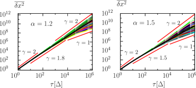
Figure 1: Time averaged mean squared displacement $\overline{\delta x^{2}}$ obtained from 400 trajectories for $\alpha=1.2$ (top) and $\alpha=1.5$ (bottom). Full red lines depict different scaling behaviors as indicated, the full black lines are averages over all trajectories.

In our simulations we use the concrete form $\psi(t)=\alpha(1+t)^{-(1+\alpha)}$ for the waiting time distribution. From this asymptotic power-law we generate $M=10^{4}$ time series of particle coordinates $x_{j}(t)$, where $j$ labels different trajectories. We calculate the ensemble averaged MSD $\langle\Delta x^{2}(\tau)\rangle=M^{-1}\sum_{j=1}^{M}x_{j}(\tau)^{2}$ and the time averaged MSD through Eq. (1). Fig. 1 shows typical results for $\overline{\delta x^{2}}$ for 400 different trajectories of duration $T=10^{8}$ time steps ($\Delta$) for $\alpha=1.2$ and $\alpha=1.5$. Remarkably, while $\overline{\delta x^{2}}$ for all trajectories coincides and shows superdiffusive scaling at shorter lag times, at longer $\tau$, $\overline{\delta x^{2}}$ displays a wide spread of slopes ranging from ballistic motion to subdiffusion ($\gamma<1$). At the same time the ensemble-averaged MSD predicts a unique long-time scaling of the form $\langle x^{2}(t)\rangle\simeq t^{3-\alpha}$, confirmed by our simulations (not shown here). Thus ergodicity, the equivalence of long time and ensemble average is broken. Moreover, self-averaging does not take place. In contrast to subdiffusive CTRW with diverging mean waiting time, where the scaling is identical for all trajectories but the generalized diffusion coefficient becomes a random variable yonghe ; pt , here we observe that the scaling exponent of individual trajectories appears random. We note that this effect is not due to bad statistics at larger $\tau$ as $\tau\ll T$ is fulfilled for all $\tau$ shown in Fig. 1. Performing an average over all trajectories, $\langle\overline{\delta x^{2}}\rangle$, the full black lines in Fig. 1, the result seems to follow the scaling predicted by Eq. (2). However, this agreement is only apparent, see below.

We first quantify the deviations between different trajectories in terms of the distribution of $\overline{\delta^{2}}$ around the trajectory-to-trajectory average $\langle\overline{\delta x^{2}}\rangle$,

$$P(\xi|\tau)=\left<\delta\left(\frac{\overline{\delta x^{2}(\tau)}}{\langle\overline{\delta x^{2}(\tau)}\rangle}-\xi\right)\right>.$$ (3)

The results for $\alpha=1.2$ and $\alpha=1.5$ are shown in Fig. 2 (Left). In the case of an infinite trajectory we would find a sharp peak at $\xi=1$, which is approximately observed for the shortest $\tau$. In contrast for finite-time trajectories $P(\xi|\tau)$ apparently relaxes towards a skewed limiting distribution with a maximum well below the ergodic value $\xi=1$. Therefore the average value appears to be dominated by one or few very long waiting time events locked onto a given velocity mode, and the self-averaging is not fulfilled. In addition we measure the long-time scaling in individual trajectories by least-squares fit of the last decade of $\overline{\delta x^{2}}$ to the power-law $t^{\alpha_{\mathrm{app}}}$, obtaining the scatter distribution of the apparent scaling exponent $\alpha_{\mathrm{app}}$. The resulting distributions $P(\alpha_{\mathrm{app}})$ for $\alpha=1.2$ and $\alpha=1.5$ are shown in Fig. 2 (Right). We see that the maximum of $P(\alpha_{\mathrm{app}})$ is well below the infinite-time average $\alpha_{\mathrm{app}}=\alpha$, and that a non-negligible fraction of trajectories in fact exhibits subdiffusion. This demonstrates that the time average of a superdiffusive dynamical process can in fact display subdiffusive behavior on the level of single trajectories of finite duration. Again, we see that finite time averages such as $\overline{\delta^{2}}$ are obviously dominated by either extremely long motion events pushing $\alpha_{\mathrm{app}}$ to values closer to $\alpha_{\mathrm{app}}=2$, while strong oscillations between velocity modes induce localization effects and values $\alpha_{\mathrm{app}}<1$. These observations will be crucial for the correct interpretation of single trajectory measurements of superdiffusive processes.

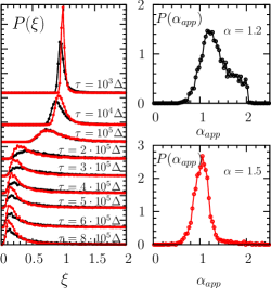
Figure 2: Left: Scatter distribution $P(\xi)$ of the time averaged MSD $\overline{\delta x^{2}}$ versus $\xi=\overline{\delta x^{2}}/\langle\overline{\delta x^{2}}\rangle$ for $\alpha=1.2$ (black) and $\alpha=1.5$ (red). Right: Scatter distribution $P(\alpha_{\mathrm{app}})$ of the apparent scaling exponent $\alpha_{\mathrm{app}}$ obtained by least-squares fit of $\overline{\delta x^{2}}\sim t^{\alpha_{\mathrm{app}}}$ to the last decade of the time series in Fig. 1.

Having established that there is no unique scaling of $\overline{\delta x^{2}}$ along finite-time single trajectories one might wonder whether and how the finiteness of single trajectories affects the corresponding average over an ensemble of trajectories. This problem can be treated exactly with the renewal approach. Once an arbitrary origin is specified on the time axis the probability that the walker is in a motion event of duration $\vartheta$ at time 0 is $p_{0}(\vartheta)d\vartheta=\vartheta\psi(\vartheta)d\vartheta/\overline{\vartheta}$, where $\overline{\vartheta}$ is the average time span of $\vartheta$ along a finite-time trajectory of duration $T$ and ensures the correct normalization, $\overline{\vartheta}=\int_{0}^{T}\vartheta\psi(\vartheta)d\vartheta\equiv\frac{1}{\alpha-1}(1-\alpha(1+\alpha T)(1+T)^{-\alpha})$. The probability that the event persists until $t$ is $p_{p}(t|\vartheta)=(\vartheta-t)/\vartheta$, such that the probability that the walker is in a motion event of duration $\vartheta$ between 0 and t is $p_{0}(\vartheta)p_{p}(t|\vartheta)d\vartheta$. The velocity autocorrelation function $C_{v}^{f}(t)$ is then obtained by averaging over all possible durations up to $T$, such that

$$C_{v}^{f}(t)=\frac{(1+t)^{1-\alpha}+(1+T)^{1-\alpha}((\alpha-1)t-(1+\alpha T))}{1-\alpha(1+\alpha T)(1+T)^{-\alpha}}$$ (4)

for $t<T$, such that for finite-time trajectories we find

$$\left<\overline{\delta x^{2}}\right>_{f}=2\frac{\frac{(1+\tau)^{3-\alpha}-1}{(3-\alpha)(2-\alpha)}-\frac{t}{2-\alpha}+\left(\frac{(\alpha-1)\tau^{3}}{6(1+T)^{\alpha}}-\frac{(1+\alpha T)\tau^{2}}{2(1+T)^{\alpha}}\right)}{(\alpha-1)\overline{\vartheta}}.$$ (5)

For long $T$ the time averaged MSD has the form

$$\left<\overline{\delta x^{2}}\right>_{f}\sim\left<\overline{\delta x^{2}}(\tau)\right>+T^{3-\alpha}\left[\frac{\alpha-1}{3}\left(\frac{t}{T}\right)^{3}-\alpha\left(\frac{t}{T}\right)^{2}\right].$$ (6)

Simulations results for $\langle\overline{\delta x^{2}}\rangle$ are shown in Fig. 3, demonstrating good agreement with the result (5). Indeed we find that on a logarithmic scale (Right, the conventional representation of time averaged MSD data) one hardly observes deviations from Eq. (2), however, on a linear scale pronounced deviations are apparent (Left). Of course as $t/T\to 1$ these deviations would become increasingly pronounced also on the logarithmic scale. To asses the importance of correction terms for given values of $\alpha$ and $T$ it is instructive to consider the ratio of $\langle\overline{\delta^{2}}\rangle>$ for finite-time and infinite-time trajectories,

$$R=\left<\overline{\delta x^{2}}\right>_{f}\Big{/}\left<\overline{\delta x^{2}}\right>$$ (7)

as function of the relative time-lag $\varphi\equiv\tau/T$. The results for various cases are shown in Fig. 4 (Left). Thus, when $\alpha=1.2$ for instance, $R(\varphi)$ decreases to 0.2 as $\varphi$ approaches 1. This finite-time depression is important in relating the amplitude of the measured time averaged MSD to the anomalous diffusion coefficient of the process. In the Brownian limit $\alpha=2$, $R(\varphi)$ is independent of the finite measurement time $T$ and equals 1.

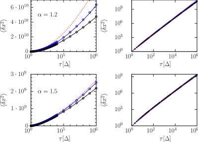
Figure 3: $\langle\overline{\delta x^{2}}\rangle$ (dashed red line) and $\langle\overline{\delta x^{2}}\rangle_{f}$ (full lines) with $T=10^{7}\Delta$ (black symbols) and $T=10^{8}\Delta$ (blue symbols). The right panel shows the same plots on the logarithmic scale.

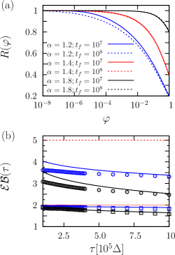
Figure 4: (a) $R(\varphi)$ for various values of $\alpha$ and $T$; (b) Ergodicity breaking parameter as function of lag time, $\mathcal{EB}(\tau)$ for $\alpha=1.2$ (circles) and $\alpha=1.5$ (squares) for $T=10^{7}\Delta$ (black) and $T=10^{8}\Delta$ (blue). The dashed and dotted red lines denote the theoretical values for infinite-time trajectories, and the full lines correspond to the predictions for the finite-time case.

Finally we investigate the nature of the ergodicity breaking and, in particular, the role of the finiteness of trajectories. As already noted by Zumofen and Klafter Zumofen2 the time averaged MSD differs from the corresponding ensemble average, thus ergodicity is broken. We define the ergodicity-breaking parameter $\mathcal{EB}(\tau)=\langle\overline{\delta x^{2}}\rangle/\langle\Delta x^{2}(\tau)\rangle$ as ratio of time versus ensemble averaged MSD REM . For our choice of $\psi(x,t)$ the ensemble averaged MSD asymptotically is $\langle\Delta x^{2}(\tau)\rangle\sim 2(\alpha-1)\tau^{3-\alpha}/((3-\alpha)(2-\alpha))$ for $1<\alpha<2$ as $\tau\to\infty$ Zumofen2 . Thus $\mathcal{EB}(\tau)=1/(\alpha-1)$ as $\tau\to\infty$, that is, time and ensemble averages differ only in terms of a constant. We call this phenomenonultraweak ergodicity breaking, in contrast to the stronger weak ergodicity breaking of scale-free subdiffusive processes. According to Eq. (5) we expect that the finiteness of trajectories will also affect $\mathcal{EB}(\tau)$. Interestingly $\mathcal{EB}(\tau)$ appears to be almost independent of $\tau$, as can bee seen in Fig. reffg4(b), but the value deviates significantly from $1/(\alpha-1)$ (dotted and dashed red lines). In fact, this is not surprising if considering the results in Fig. 3, where we found that the scaling of finite-time averages on the logarithmic scale agrees rather well with the prediction for infinite trajectories, suggesting that the correction terms effectively cause a rescaling of the generalized time-average diffusion coefficient. We might call this apparent ultraweak ergodicity breaking.

We investigated the ultraweakly ergodic behavior of superdiffusive LWs, finding a pronounced scatter of apparent scaling exponents of the time averaged MSD for finite-time trajectories. These apparent scaling exponents range between ballistic motion (sticking to one velocity mode) down to subdiffusive values (localization due to erratic hopping between different velocity modes). Moreover, averaged over many individual trajectories, the time averaged MSD is pronouncedly smaller than for very long trajectories. We quantify these effects in terms of an ergodicity breaking parameter.

The present results reveal the importance to take into account the effects of the finiteness of trajectories when interpreting experimental results. They also demonstrate how the measured time series of different lengths reveal more reliable information about the fundamental underlying dynamical process. The additional information comes from the dependence of time averaged quantities on the length of time series. Instead of attempting to measure or generate longer and longer time series to extract reliable time averaged quantities, one could instead use many shorter time series and obtain even more reliable results. Our results may also provide an alternative and more robust method of determining exponents of probability densities of step durations. Namely, since we inevitably expect poor sampling of very long events this might be reflected in the obtained exponent. Using the time averaged MSD from measurements of different (but known) durations one should in principle be able to determine the exponent more accurately.

We acknowledge funding from the Academy of Finland (FiDiPro scheme) and the German Ministry for Science and Education.

References

- (1) D. W. Sims et al., Nature 451, 1098 (2008); N. E. Humphries et al., Nature 465, 1066 (2010).
- (2) R. Nathan et al., Proc. Natl. Acad. Sci. USA 105, 19052 (2008).
- (3) M. C. González, C. A. Hidalgo, and A.-L. Barabási, Nature 453, 779 (2008); D. Brockmann, Phys. World (2), 31 (2010).
- (4) G. Ramos-Fernandez et al., Behav. Ecol. Sociobiol. 55, 223 (2003).
- (5) G. Zumofen and J. Klafter, Phys. Rev. E 47, 851 (1993).
- (6) G. Zumofen and J. Klafter, Physica D 69, 436 (1993).
- (7) T. Geisel, S. Thomae, Phys. Rev. Lett. 52, 1936 (1984).
- (8) T. H. Solomon, E. R. Weeks, and H. L. Swinney, Phys. Rev. Lett. 71, 3975 (1993); G. Zumofen and J. Klafter, Phys. Rev. E 51, 1818 )1995).
- (9) T. Geisel, J. Nierwetberg, and A. Zacherl, Phys. Rev. Lett. 54, 6161 (1985).
- (10) R. Fleischmann, T. Geisel, and R. Ketzmerick, Europhys. Lett. 25, 219 (1994).
- (11) S. Marksteiner, K. Ellinger, and P. Zoller, Phys. Rev. A 53, 3409 (1996).
- (12) P. Barthelemy, J. Bertolotti, and D. S. Wiersma, Nature 453, 495 (2008).
- (13) Y.-J. Jung, E. Barkai, and R. J. Silbey, Chem. Phys. 284, 181 (2002).
- (14) M. de Jager, F. J. Weissing, P. M. J. Herman, B. A. Nolet, and J. van de Koppel, Science 332, 1551 (2011).
- (15) T. H. Harris et al., Nature 486, 545 (2012).
- (16) E. Barkai, Y. Garini, and R. Metzler, Phys. Today 65(8), 29 (2012).
- (17) Y. He, S. Burov, R. Metzler, and E. Barkai, Phys. Rev. Lett. 101, 058101 (2008); S. Burov, J.-H. Jeon, R. Metzler, and E. Barkai, Phys. Chem. Chem. Phys. 13, 1800 (2011).
- (18) W. Deng and E. Barkai, Phys. Rev. E 79, 011112 (2009); I. Goychuk, ibid. 80, 046125 (2009); J.-H. Jeon and R. Metzler, ibid. 81, 021103 (2010).
- (19) Note that even ergodic anomalous diffusion processes may show non-ergodic features under confinement, see J.-H. Jeon, R. Metzler, Phys. Rev. E 85, 021147 (2012).
- (20) A. V. Weigel et al., Proc. Nat. Acad. Sci. USA 108, 6438 (2011).
- (21) J.-H. Jeon et al., Phys. Rev. Lett. 106, 048103 (2011).
- (22) M. F. Shlesinger, J. Klafter, and Y. M. Wong, J. Stat. Phys. 27, 499 (1982).
- (23) E. W. Montroll and G. H. Weiss, J. Math. Phys. 10, 753 (1969); H. Scher and E. W. Montroll, Phys. Rev. B 12, 2455 (1975).
- (24) J. Klafter, A. Blumen, and M. F. Shlesinger, Phys. Rev. A 35, 3081 (1987).
- (25) J. Klafter, M. F. Shlesinger, and G. Zumofen, Phys. Today 49, 33 (1996).
- (26) R. Metzler and J. Klafter, Phys. Rep. 339, 1 (2000); J. Phys. A 37, R161 (2004).
- (27) G. Trefán, E. Floriani, B. J. West, and P. Grigolini, Phys. Rev. E 50, 2564 (1994).
- (28) I. M. Sokolov and R. Metzler, Phys. Rev. E 67, 010101 (2003).
- (29) M. Magdziarz, W. Szczotka, and Zebrowski, J. Stat. Phys. 147, 74 (2012).
- (30) R. Kubo, Rep. Prog. Phys. 29, 255 (1966); J.-P. Hansen, I.R. McDonald, Theory of simple liquids, 3rd. Ed., (Academic Press, Amsterdam, 2006).
- (31) Note the difference to the definition of the ergodicity breaking parameter introduced previously yonghe ; pt .