Thermodynamics of the two-dimensional frustrated $J_{1}$-$J_{2}$ Heisenberg ferromagnet in the collinear stripe regime: Susceptibility and correlation length

Abstract

We calculate the temperature dependence of the correlation length $\xi$ and the uniform susceptibility $\chi_{0}$ of the frustrated $J_{1}$-$J_{2}$ square-lattice Heisenberg ferromagnet in the collinear stripe phase using Green-function technique. The height $\chi_{max}$ and the position $T(\chi_{max})$ of the maximum in the $\chi_{0}(T)$ curve exhibit a characteristic dependence on the frustration parameter $J_{2}/|J_{1}|$, which is well described, for $J_{2}>0.7|J_{1}|$, by the relations $\chi_{max}=a\left(J_{2}-J_{2}^{c}\right)^{-\nu}$ and $T(\chi_{max})=b(J_{2}-J_{2}^{c})$, where $J_{2}^{c}=0.4|J_{1}|$ and $\nu$ is of the order of unity. The correlation length diverges at low temperatures as $\xi\propto e^{A/T}$, where $A$ increases with growing $J_{2}/|J_{1}|$. We also compare our results with recent measurements on layered oxovanadates and find reasonable agreement.

I Introduction

Frustrated square-lattice quantum magnets have been in the focus of active condensed-matter investigations in recent years. While for the study of ground state (GS) properties many alternative methods, such as exact diagonalization (ED),schulz ; shannon06 ; ED40 ; richter10 the Schwinger boson approach,feldner11 functional renormalization group method,reuther10 the tensor-product approach,Verstraete:2011 or the coupled-cluster method (CCM)richter10 can be applied, there are much less reasonable theoretical approaches available to deal with thermodynamic properties of these systems. On the other hand, there are many recent experimental studies on quasi-two-dimensional frustrated square-lattice compounds, see, e.g., Refs. kaul04, ; enderle, ; nath, ; rosner09, ; rosner09a, ; nath08, ; carretta2009, ; carretta2011, ; tsirlin2011, ; johnston2011, , where typically temperature dependent properties are reported, which should be compared with theoretical predictions. The quantum Monte Carlo technique is not applicable due to the sign problem for frustrated systems.troyer2005 The high-temperature expansion approachRosner_HTE ; schmidt11 is limited to temperatures down to the order of the exchange coupling. Full ED studies used in Refs. shannon04, ; schmidt07, ; schmidt07_2, for the $J_{1}$-$J_{2}$ square-lattice Heisenberg ferromagnet of $N=8,16$ and $20$ sites suffer from finite-size effects at lower temperatures.haertel10 ; schmidt11 An alternative method to describe quantum magnets in the whole temperature range is the Green-function technique.elk ; froebrich06 ; rudoy2011 A rotationally invariant second-order Green-function theory has been applied successfully to describe the thermodynamics of frustrated quantum magnets.barabanov94 ; ihle2001 ; barabanov2009 ; haertel08 ; haertel10 ; barabanov2011 In particular, the Green-function technique is designed for $N\to\infty$ and allows the calculation of the magnetic correlation length, in addition to the usual thermodynamic quantities, such as the susceptibility.

Motivated by recent measurements of the correlation lengths for several frustrated layered Heisenberg square-lattice ferromagnets,carretta2011 in the present paper we study the temperature dependence of the correlation length and the uniform susceptibility of the spin-1/2 $J_{1}$-$J_{2}$ model

$$H=J_{1}\sum_{\langle i,j\rangle}{\bf S}_{i}{\bf S}_{j}+J_{2}\sum_{\langle\langle i,j\rangle\rangle}{\bf S}_{i}{\bf S}_{j},$$ (1)

where $\langle\ldots\rangle$ denotes the nearest neighbor (NN) and $\langle\langle\ldots\rangle\rangle$ the next-nearest neighbor (NNN) bonds on a square lattice. We consider a ferromagnetic NN coupling $J_{1}<0$ and a frustrating antiferromagnetic NNN coupling $J_{2}>0$. The GS of this model has been discussed in Refs. shannon06, ; richter10, ; feldner11, . At $J_{2}=J_{2}^{c}\approx 0.4|J_{1}|$ the ferromagnetic GS present at small $J_{2}$ gives way for a GS phase with zero total magnetization. Although, the nature of this state for $J_{2}\gtrsim J_{2}^{c}$ is still under debate, the existence of antiferromagnetic collinear stripe GS long-range order (LRO) for $J_{2}>0.7|J_{1}|$ is not questioned.

Following our previous investigation of this model, see Ref. haertel10, , we use the rotationally invariant second-order Green-function method (RGM) to calculate the thermodynamic properties. However, by contrast to Ref. haertel10, , where the model was studied in the ferromagnetic regime, i.e. $J_{2}<J_{2}^{c}$, here we focus on the antiferromagnetic collinear stripe GS regime. We restrict our study on the parameter region $J_{2}>0.7|J_{1}|$, that corresponds to the experimental situation for several layered oxovanadates.kaul04 ; nath08 ; carretta2011

The paper is organized as follows. In Sec. II the RGM applied to the $J_{1}$-$J_{2}$ square lattice is illustrated. The results for the susceptibility and correlation length and the comparison to recent experimental data is presented in Sec. III. Finally, a short summary is given in Sec. IV.

II Rotationally invariant Green-function method (RGM)

The RGM was introduced by Kondo and Yamaji.kondo The method was further developed and applied to Heisenberg magnets by several groups, see, e.g., Refs. shimahara91, ; SSI94, ; barabanov94, ; winterfeldt97, ; schindelin1999, ; Yu2000, ; ihle2001, ; canals2002, ; schmal2004, ; schmal06, ; barabanov2009, ; haertel08, ; junger3d, ; ihle2008, ; haertel10, ; barabanov2011, .

To calculate the dynamical transverse spin susceptibility $\chi_{q}^{+-}\left(\omega\right)$ we have to determine the two-time commutator Green function $\langle\langle S_{q}^{+};S_{-q}^{-}\rangle\rangle_{\omega}=-\chi_{q}^{+-}\left(\omega\right)$. The equation of motion for $\langle\langle S_{q}^{+};S_{-q}^{-}\rangle\rangle_{\omega}$ up to second order reads $\omega^{2}\langle\langle S_{q}^{+};S_{-q}^{-}\rangle\rangle_{\omega}=M_{q}+\langle\langle-\ddot{S}_{q}^{+};S_{-q}^{-}\rangle\rangle_{\omega}$ with $-\ddot{S}_{q}^{+}=\left[\left[S_{q}^{+},H\right],H\right]$ and the exact moment

$$M_{q}=-8J_{1}C_{1,0}\left(1-\gamma_{q}^{(1)}\right)-8J_{2}C_{1,1}\left(1-\gamma_{q}^{(2)}\right),$$ (2)

where $\gamma_{q}^{(1)}=\left(\cos q_{x}+\cos q_{y}\right)/2$ and $\gamma_{q}^{(2)}=\cos q_{x}\cos q_{y}$. $C_{n,m}$ denotes the correlation functions. Assuming rotational symmetry, i.e., $\langle S_{i}^{z}\rangle=0$, they read $C_{n,m}=C_{\bf R}=\langle S_{\bf R}^{-}S_{0}^{+}\rangle=2\langle S_{\bf R}^{z}S_{0}^{z}\rangle$ with ${\bf R}=n{\bf e}_{x}+m{\bf e}_{y}$. Calculating the second derivative $-\ddot{S}_{q}^{+}$, an approximation as indicated in Refs. haertel08, ; haertel10, ; kondo, ; shimahara91, ; SSI94, ; barabanov94, ; ihle2001, ; winterfeldt97, ; schindelin1999, ; Yu2000, ; canals2002, ; schmal2004, ; schmal06, ; junger3d, ; ihle2008, ; barabanov2009, ; barabanov2011, is used which implies the decoupling scheme

$$S_{i}^{+}S_{j}^{+}S_{k}^{-}=\alpha_{i,k}\langle S_{i}^{+}S_{k}^{-}\rangle S_{j}^{+}+\alpha_{j,k}\langle S_{j}^{+}S_{k}^{-}\rangle S_{i}^{+},$$ (3)

where the quantities $\alpha_{i,k}$ are vertex parameters introduced to improve the decoupling scheme. In the vicinity of $J_{2}^{c}$ a spin nematic phase could be present, and the decoupling scheme (3) might be not appropriate. Therefore, we restrict our consideration to sufficiently large values of $J_{2}$, $J_{2}>0.7|J_{1}|$, where the semi-classical antiferromagnetic collinear stripe GS LRO is present. Since an $\alpha_{i,k}$ is a function of the lattice vector ${\bf R}_{i}-{\bf R}_{k}$ connecting the sites $i$ and $k$, in what follows we use the same notation as for the correlation functions $C_{n,m}$, i.e. the vertex parameter $\alpha_{n,m}$ belongs to the lattice vector ${\bf R}=n{\bf e}_{x}+m{\bf e}_{y}$. We obtain $-\ddot{S}_{\bf q}^{+}=\omega_{\bf q}^{2}S_{\bf q}^{+}$ and

$$\chi_{\bf q}^{+-}\left(\omega\right)=-\langle\langle S_{\bf q}^{+};S_{-{\bf q}}^{-}\rangle\rangle_{\omega}=\frac{M_{\bf q}}{\omega_{\bf q}^{2}-\omega^{2}},$$ (4)

with

$$\omega_{\bf q}^{2} =2\sum_{k,l(=1,2)}J_{k}J_{l}\left(1-\gamma_{\bf q}^{(k)}\right)\times$$

$$\left[K_{k,l}+8\alpha_{1,k-1}C_{1,k-1}\left(1-\gamma_{\bf q}^{(l)}\right)\right],$$ (5)

where $K_{1,1}=1+2\left(2\alpha_{1,1}C_{1,1}+\alpha_{2,0}C_{2,0}-5\alpha_{1,0}C_{1,0}\right)$, $K_{2,2}=1+2\left(2\alpha_{2,0}C_{2,0}+\alpha_{2,2}C_{2,2}-5\alpha_{1,1}C_{1,1}\right)$, $K_{1,2}=4\left(\alpha_{1,2}C_{1,2}-\alpha_{1,0}C_{1,0}\right)$, and $K_{2,1}=4\left(\alpha_{1,0}C_{1,0}+\alpha_{1,2}C_{1,2}-2\alpha_{1,1}C_{1,1}\right)$. The correlation functions $C_{n,m}$ are calculated using the spectral theorem,elk

$$C_{\bf q}=\langle S_{\bf q}^{+}S_{\bf q}^{-}\rangle=\frac{M_{\bf q}}{2\omega_{\bf q}}\left[1+2n\left(\omega_{\bf q}\right)\right],$$ (6)

where $n(\omega_{\bf q})=\left(e^{\omega_{\bf q}/T}-1\right)^{-1}$ is the Bose function.
Magnetic LRO is reflected by a non-vanishing condensation term $C$ (see, e.g., Refs. shimahara91, ; winterfeldt97, ; ihle2001, ) according to $C_{\bf{R}}=\frac{1}{N}\sum_{{\bf q}\neq{\bf Q}}C_{\bf q}e^{i{\bf q}\bf{R}}+Ce^{i{\bf Q}\bf{R}}$ where ${\bf Q}$ denotes the magnetic ordering vector. The magnetic order parameter (sublattice magnetization) is calculated as

$$m^{2}=\frac{3}{2}\frac{1}{N}\sum_{\bf R}C_{\bf R}e^{-i{\bf Q}{\bf R}}=\frac{3}{2}C.$$ (7)

The corresponding static susceptibility is given by $\chi_{\bf Q}=\frac{1}{2}\lim_{{\bf q}\to{\bf Q}}\chi_{\bf q}^{+-}\left(\omega=0\right)$. The uniform static susceptibility is $\chi_{0}=\frac{1}{2}\chi^{+-}_{\bf q=0}(\omega=0)$. The correlation length is obtained by an expansion of the static susceptibility around the magnetic ordering vector ${\bf Q}$, $\chi^{+-}_{{\bf Q}+{\bf q}}\approx\chi^{+-}_{{\bf Q}}\left(1-\xi_{x}^{2}q_{x}^{2}-\xi_{y}^{2}q_{y}^{2}\right)$, see, e.g., Refs. winterfeldt97, ; ihle2001, ; schmal2004, ; haertel08, ; haertel10, . From the on-site correlator $\langle S_{i}^{-}S_{i}^{+}\rangle$ and the operator identity $S_{i}^{-}S_{i}^{+}=\frac{1}{2}+S_{i}^{z}$ we get the sum rule

$$C_{0}=\frac{1}{N}\sum_{\bf q}C_{\bf q}=\frac{1}{2}.$$ (8)

Considering the collinear stripe phase we have two equivalent magnetic ordering vectors, ${\bf Q}_{1}=\left(0,\pi\right)$ and ${\bf Q}_{2}=\left(\pi,0\right)$. To preserve square-lattice symmetry we follow Ref. ihle2001, and calculate the correlation functions as $C_{n,m}=\left(C^{(1)}_{n,m}+C^{(2)}_{n,m}\right)/2$ with $C^{(i)}_{n,m}=\frac{1}{N}\sum_{{\bf q}\neq{\bf Q}_{i}}C_{\bf q}e^{i{\bf q}\bf{R}}+Ce^{i{\bf Q}_{i}\bf{R}}$. Note that $C$ is the same for ${\bf Q}_{1}$ and ${\bf Q}_{2}$. Analogously, we consider $\chi_{{\bf Q}+{\bf q}}=\left(\chi_{{\bf Q}_{1}+{\bf q}}+\chi_{{\bf Q}_{2}+{\bf q}}\right)/2$ to get the correlation length by expansion of $\chi_{{\bf Q}+{\bf q}}$ for small ${\bf q}$ yielding

$$\xi^{2} =\frac{2J_{2}C_{1,1}}{4J_{1}C_{1,0}+8J_{2}C_{1,1}}+\frac{A}{\Delta},$$ (9)

where $\Delta=2J_{1}^{2}K_{1,1}+4J_{2}^{2}K_{2,2}+2J_{1}J_{2}\left(K_{1,2}+2K_{2,1}\right)+16\left(J_{1}+2J_{2}\right)\left(J_{1}\alpha_{1,0}C_{1,0}+2J_{2}\alpha_{1,1}C_{1,1}\right))$ and $A=-J_{2}^{2}\left(32\alpha_{1,1}C_{1,1}+K_{2,2}\right)-4J_{1}J_{2}\left(3\alpha_{1,0}C_{1,0}+\alpha_{1,2}C_{1,2}\right)$.

In the GS, LRO may exist, that is, $C\neq 0$. $C$ is determined byshimahara91 ; schindelin1999 ; schmal06 $\chi^{-1}_{{\bf Q}_{1}}=\chi^{-1}_{{\bf Q}_{2}}=0$ with

$$\chi_{{\bf Q}_{i}}=-\frac{-4J_{1}C_{1,0}-8J_{2}C_{1,1}}{\Delta}.$$ (10)

Next we have to discuss the choice of the vertex parameters $\alpha_{n,m}$. Obviously, there are five different $\alpha_{n,m}$ in Eq. (II) which have to be determined together with the corresponding correlation functions $C_{n,m}$. In addition, at zero temperature the condensation term $C$ (describing magnetic LRO) has to be considered. To determine these quantities we can use the Fourier transformation of Eq. (6) providing five equations for $C_{n,m}$. Moreover, at zero temperature we use $\chi^{-1}_{{\bf Q}_{1}}=\chi^{-1}_{{\bf Q}_{2}}=0$ to calculate $C$, see above. Finally, only one equation, namely the sum rule (8), is left to find the vertex parameters. Hence, we have to introduce further approximations. In the case of a ferromagnetic GS ($J_{2}<J_{2}^{c}$) all correlation functions behave quite similar and a reasonable approximation is to set $\alpha_{n,m}=\alpha$, see, e.g., Refs. shimahara91, ; haertel08, and haertel10, . This simple approximation was also used in Ref. kondo, applying the RGM to antiferromagnets. However, in the antiferromagnetic regime the correlation functions carry different signs, and setting $\alpha_{n,m}=\alpha$ leads to poor results at low temperatures. A significant improvement of the RGM results for antiferromagnets can be achieved by introducing two independent vertex parameters.shimahara91 ; ihle2001 ; schmal06 This requires, however, an additional external input to get one more equation. To take into account the dominant character of $J_{2}$ in the collinear stripe phase, we set $\alpha_{1,1}=\alpha_{1}$ and $\alpha_{n,m}=\alpha_{2}$, $(n,m)\neq(1,1)$. Since the low-temperature properties of the model are related to excitations above the GS, a realistic description of the GS is necessary. Therefore, in the present paper we use, as an additional external input, the GS sublattice magnetization calculated by the CCM.richter10 Thus, describing GS magnetic ordering properly, we may expect that the RGM provides also a reasonable description of the low-temperature properties of the model. This input yields the required additional equation to determine the two independent vertex parameters $\alpha_{1}$ and $\alpha_{2}$ at $T=0$. As a result we can also calculate the uniform static susceptibility $\chi_{0}$ at $T=0$, cf. Fig. 1.

For finite temperatures we need a reasonable ansatz for the temperature dependence of the ratio $\alpha_{2}/\alpha_{1}$ of the vertex parameters, see, e.g. Refs. winterfeldt97, ; shimahara91, ; ihle2001, and junger3d, . We have tested several ansatzes to a get a proper description of thermodynamic quantities in the whole temperature range, see below. To solve the system of RGM equations we use Broyden’s method,NR3 which yields the solutions with a relative error of about $10^{-8}$ on the average. The momentum integrals are done by Gaussian integration. To find the numerical solution of the equations for $T>0$, we start at high temperatures and decrease $T$ in small steps. Below a certain (low) temperature $T_{0}(J_{2})$ no solutions of the RGM equations (except at $T=0$) could be found, since the quantity $\Delta(T,J_{2})$ in Eqs. (9) and (10) becomes exponentially small which leads to numerical instabilities. As expected, at large temperatures the concrete choice of the ratio $\frac{\alpha_{2}}{\alpha_{1}}(T)$ becomes irrelevant, and even the simple approximation $\alpha_{n,m}=\alpha$ yields results for $\chi_{0}(T)$ which coincide with the data from the high-temperature expansion. At low temperatures a resonable ansatz for the ratio $\alpha_{2}/\alpha_{1}$ should (i) provide numerical data down to sufficiently low temperatures and (ii) yield coincidence of $\chi_{0}(T=0)$ determined by using the CCM input and $\lim_{T\to 0}\chi_{0}(T)$ calculated with the ansatz for $\frac{\alpha_{2}}{\alpha_{1}}(T)$. The simplest way is to fix the ratio $\frac{\alpha_{2}}{\alpha_{1}}$ to its value at $T=0$. Tracing the RGM solution to very low temperatures we find that the ansatz

$$\frac{\alpha_{2}(T)}{\alpha_{1}(T)}=1+\left(\frac{\alpha_{2}(0)}{\alpha_{1}(0)}-1\right)e^{-\gamma T}\;,\;\gamma\geq 0$$ (11)

with the tiny exponent $\gamma=0.005$ is more appropriate to get numerically stable solutions at low $T$. Note, however, that our results are not noticeably influcenced by the choice of $\gamma$, see also Fig. 1. In what follows we use this ansatz to solve the RGM equations with two vertex parameters.

Figure 1: Uniform susceptibility $\chi_{0}$ of the $J_{1}$-$J_{2}$ model for ferromagnetic $J_{1}=-1$.
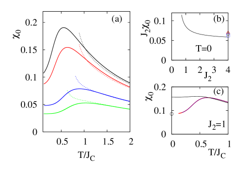
(a) Temperature dependence of the uniform susceptibility $\chi_{0}$ for $J_{2}=0.9$ (black), $J_{2}=1.0$ (red), $J_{2}=1.5$ (blue), and $J_{2}=2.0$ (green) calculated by RGM (solid lines). The temperature $T$ is scaled by $J_{C}=\sqrt{J_{1}^{2}+J_{2}^{2}}$. For comparison, eighth-order high-temperature expansion results (Refs. Rosner_HTE, ; schmidt11, ) are shown (dashed lines).
(b) Ground-state values for $J_{2}\chi_{0}$ vs. $J_{2}$. The susceptibility data for the square-lattice antiferromagnet (quantum Monte Carlorunge92 - black circle, CCMfarnell09 - red triangle, third-order spin-wave theoryhamer92 - blue square) are also shown as data points at $J_{2}=4$.
(c) Comparison of the temperature dependence of the uniform susceptibility $\chi_{0}$ for $J_{2}=1$ calculated using three different choices of the vertex parameters (red line - two vertex parameters with the ansatz (11) and $\gamma=0.005$, blue line - two vertex parameters with fixed ratio $\frac{\alpha_{2}}{\alpha_{1}}(T)=\frac{\alpha_{2}}{\alpha_{1}}(0)$ (i.e. ansatz (11) with $\gamma=0$), black line - only one vertex parameter). Note that the red and the blue lines practically coincide. Note further that the red line extends down to slightly lower temperatures. The black circle at $T=0$ shows the zero-temperature RGM value for $\chi_{0}$ calculated with two vertex parameters.

III Results and Discussion

In what follows we fix the ferromagnetic NN exchange to $J_{1}=-1$. We focus on sufficiently large values of $J_{2}$, $J_{2}>0.7$, where a possible nematic GS phase is not present, and, rather the GS exhibits semi-classical collinear magnetic LRO. Moreover, the experimental data for layered oxovanadateskaul04 ; nath08 ; carretta2011 correspond to this parameter regime. We follow Ref. shannon04, and use as a characteristic energy scale $J_{C}=\sqrt{J_{1}^{2}+J_{2}^{2}}$, see also Refs. nath08, ; carretta2011, .

In Fig. 1(a) the temperature dependence of the uniform susceptibility $\chi_{0}$ is shown. For comparison we also present the results of the eighth order high-temperature expansion,schmidt11 which agree with the RGM data at large $T$. In Fig. 1(b) the GS results for the susceptibility $\chi_{0}(T=0)$ are presented. Since for large $J_{2}$ the $J_{1}$-$J_{2}$ model corresponds to a system of two inter-penetrating square-lattice antiferromagnets with coupling strength $J_{2}$, our RGM data for $\chi_{0}(T=0)$ can be compared with available GS results for $\chi_{0}(T=0)$ of the square-lattice antiferromagnet,runge92 ; hamer92 ; farnell09 see data points at $J_{2}=4$ in Fig. 1(b). For large $J_{2}$, the dependence of $J_{2}\chi_{0}(T=0)$ on $J_{2}$ is weak down to $J_{2}\sim 1$. A noticeable upturn of $J_{2}\chi_{0}(T=0)$ for small $J_{2}$ may indicate the approach to the ferromagnetic phase. In Fig. 1(c) we compare different choices of the vertex parameters to solve the RGM equations, see the discussion in Sec. II. Obviously, the use of only one vertex parameter by setting $\alpha_{n,m}=\alpha$ leads to poor results for $T\lesssim 0.6J_{C}$. On the other hand, the two choices of the parameter $\gamma$ in the ansatz (11) lead to almost identical $\chi_{0}(T)$ curves.

Figure 2: Height and position of the maximum of the susceptibility $\chi_{0}(T)$ for the $J_{1}$-$J_{2}$ model with $J_{1}=-1$ in dependence on the frustration parameter $J_{2}$. The blue circles are the RGM results, the open squares show the ED data for $N=16$, the lines correspond to Eqs. (12) and (13), and the colored filled symbols correspond to BaCdVO(PO₄)₂ ($J_{2}/|J_{1}|\approx 0.9$)nath08 , SrZnVO(PO₄)₂ ($J_{2}/|J_{1}|\approx 1.15$)carretta2011 , and Pb₂VO(PO₄)₂ ($J_{2}/|J_{1}|\approx 1.8$).kaul04

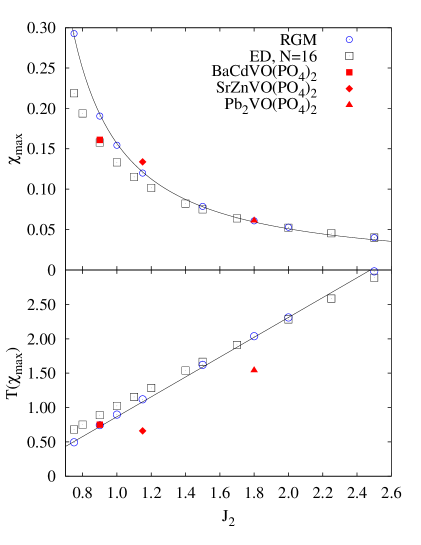
For the comparison with experimental data on oxovanadate compounds, such as BaCdVO(PO₄)₂, SrZnVO(PO₄)₂, and Pb₂VO(PO₄)₂ kaul04 ; nath08 ; carretta2011 , the height $\chi_{max}$ and the position $T(\chi_{max})$ of the maximum in the $\chi_{0}(T)$ curve are interesting features. However, in these compounds, due to a weak interlayer coupling, a phase transition to magnetic long-range order at a critical temperature $T_{N}$ was detected,kaul04 ; nath08 ; carretta2011 where $T_{N}/|J_{1}|\sim 0.28,0.35$, and $0.48$ was found for BaCdVO(PO₄)₂, SrZnVO(PO₄)₂, and Pb₂VO(PO₄)₂, respectively. Since in our paper we deal with a strictly two-dimensional model, such a comparison is reasonable only in the paramagnetic phase of the compounds, i.e. at $T>T_{N}$, where two-dimensional spin physics dominates the thermodynamic behavior. Indeed, the relevant temperatures $T(\chi_{max})$ are well above $T_{N}$ for all three oxovanadates, namely $T(\chi_{max})/|J_{1}|=0.75,0.66$, and $1.54$ for BaCdVO(PO₄)₂, SrZnVO(PO₄)₂, and Pb₂VO(PO₄)₂, respectively, see Fig. 2.

We mention, that $\chi_{max}$ and $T(\chi_{max})$ have been presented as fuctions of $\tan^{-1}(J_{2}/J_{1})$ for the whole parameter space of $J_{1}$ and $J_{2}$ in Ref. shannon04, using full ED for $N=8,16$ and $20$ sites, see Fig. 17 in Ref. shannon04, . We have recalculated the corresponding ED data for $N=16$. In Fig. 2 we show the ED and the RGM results for $\chi_{max}$ and $T(\chi_{max})$ as functions of $J_{2}$ in the parameter region $J_{2}>0.7$ considered in our paper.

The RGM data points are well described by the relations

$$\chi_{max} =a\left(J_{2}-J_{2}^{c}\right)^{-\nu},$$ (12)

$$T(\chi_{max}) =b(J_{2}-J_{2}^{c})$$ (13)

with $a=0.0872$, $\nu=1.146$, $b=1.444$, and $J_{2}^{c}=0.4$. Note, however, that the divergence of $\chi_{max}$ at $J_{2}^{c}=0.4$ suggested by Eq. (12) might be absent in the considered model, since our approach is not designed for $J_{2}\sim J_{2}^{c}$. Using experimental data of the susceptibility for quasi-two-dimensional frustrated square-lattice magnets as well as the reported exchange constants $J_{1}$ and $J_{2}$ we can compare our theoretical data directly with experiment, see Fig. 2. Obviously, theory and experiment agree well, particularly for $\chi_{max}$. Hence, our equations (12) and (13) can be used to get information on the ratio $J_{2}/|J_{1}|$ from susceptibility measurements.

Figure 3: Temperature dependence of the correlation length $\xi$ (in units of the lattice spacing) for different values of the frustration parameter $J_{2}$=0.9, 1.0, 1.5, 2.0 and 2.5 (from left to right). The temperature $T$ is scaled by $J_{C}=\sqrt{J_{1}^{2}+J_{2}^{2}}$. The inset shows the correlation length for $T=0.4$ in dependence on the frustration parameter $J_{2}$. The solid line represents a fit to the data points (open squares).

Figure 4: Spin stiffness $\rho_{s}$ of the $J_{1}$-$J_{2}$ model for ferromagnetic $J_{1}=-1$ as a function of $J_{2}$ calculated by the CCM.

Figure 5: Correlation length $\xi$ (logarithmic scale) in units of the lattice spacing vs. $J_{2}/T$ calculated using RGM (lines) for various values of the frustration parameter $J_{2}$. For comparison we also show experimental datacarretta2011 for BaCdVO(PO₄)₂ ($J_{2}/|J_{1}|\approx 0.9$), SrZnVO(PO₄)₂ ($J_{2}/|J_{1}|\approx 1.15$), and Pb₂VO(PO₄)₂ ($J_{2}/|J_{1}|\approx 1.8$).

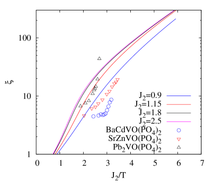
Next we discuss the correlation length $\xi$. Its temperature dependence is depicted in Fig. 3 for different values of the frustration parameter $J_{2}$. With increasing NNN exchange $J_{2}$ the rapid increase in $\xi$ is shifted to larger temperatures. As shown in the inset of Fig. 3, at a certain fixed temperature, $\xi$ decreases rapidly with decreasing $J_{2}$.

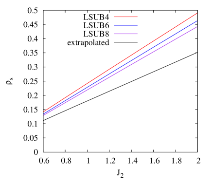
The exponential low-temperature divergence of $\xi\propto e^{A/T}$ for two-dimensional Heisenberg magnets with NN interactions is determined by the spin stiffness $\rho_{s}$, i.e. $A\propto\rho_{s}$, see e.g. Refs. kopietz, ; auerbach, ; chakravarty, ; hasenfratz, ; greven, ; haertel10, . As it has been recently reported,haertel10 for small $J_{2}$, where a ferromagnetic GS is present, the relation $\xi\propto e^{a\rho_{s}/T}$ also holds if the NNN exchange $J_{2}$ is included. In this case the stiffness was obtained from the RGM dispersion relationhaertel10 as $\rho_{s}^{FM}=-(J_{1}+2J_{2})/4$. For the antiferromagnetic collinear stripe GS phase present at large $J_{2}$ one may expect that the stiffness also determines the exponential divergence at small $T$. However, the determination of $\rho_{s}$ is more difficult. Here we use the CCMbishop04 ; krueger06 ; darradi08 to provide data for $\rho_{s}$. To calculate $\rho_{s}$ within the CCM we follow strictly Refs. krueger06, and darradi08, and do not explain details of the calculation. The stiffness as a function of $J_{2}$ is shown in Fig. 4 for various levels of CCM approximations, LSUB$n$, as well as extrapolated data.lsubn The obvious (almost) linear $J_{2}$-dependence of $\rho_{s}$ is well described for the extrapolated CCM data by $\rho_{s}\approx 0.175J_{2}$. Hence, it seems to be reasonable to show the temperature dependence of the correlation length, in addition to Fig. 3, as a function $\ln\xi(J_{2}/T)$, see Fig. 5. First we notice that the experimental data reported in Ref. carretta2011, agree reasonably well with our RGM results. Secondly, it is obvious that for large values of $J_{2}\gtrsim 1.5$ the $\ln\xi(J_{2}/T)$ curves almost coincide. The small deviations can be attributed to a temperature dependent prefactor in front of the exponential term.kopietz ; auerbach ; chakravarty ; hasenfratz ; greven ; haertel10 However, for $J_{2}=1.15$ and $J_{2}=0.9$ the theoretical as well as the experimental data show deviations from the behavior suggested by the stiffness data.

IV Summary

Using second-order Greens function technique we have calculated the uniform susceptibility $\chi_{0}$ and the correlation length $\xi$ of the frustrated $J_{1}$-$J_{2}$ square-lattice Heisenberg ferromagnet in the collinear antiferromagnetic regime present for large values of $J_{2}/|J_{1}|$. We have derived simple power laws for the height and the position of the maximum in the $\chi_{0}(T)$ curve as functions of $J_{2}$. We have found that our theoretical data agree reasonably well with recent experiments on oxovanadates.

Acknowledgment The authors are indebted to O. Derzhko for critical reading of the manuscript.
J.R. and S.-L.D. thank the DFG for financial support (grants DR269/3-3 and RI615/16-3).

References

- (1) H. J. Schulz and T. A. L. Ziman, Europhys. Lett. 18, 355 (1992); H. J. Schulz, T. A. L. Ziman, and D. Poilblanc, J. Phys. I 6, 675 (1996).
- (2) N. Shannon, T. Momoi, and P. Sindzingre, Phys. Rev. Lett. 96, 027213 (2006).
- (3) J. Richter and J. Schulenburg, Eur. Phys. J. B 73, 117 (2010).
- (4) J. Richter, R. Darradi, J. Schulenburg, D. J. J. Farnell, and H. Rosner, Phys. Rev. B 81, 174429 (2010).
- (5) H. Feldner, D. C. Cabra, and G. L. Rossini, Phys. Rev. B 84, 214406 (2011).
- (6) J. Reuther and P. Wölfle, Phys. Rev. B 81, 144410 (2010).
- (7) Ling Wang, Zheng-Cheng Gu, Xiao-Gang Wen, and F. Verstraete, arXiv:1112.3331
- (8) E. E. Kaul, H. Rosner, N. Shannon, R.V. Shpanchenko, and C. Geibel, J. Magn. Magn. Mater. 272-276(II), 922 (2004).
- (9) R. Nath, A.A. Tsirlin, H. Rosner, and C. Geibel, Phys. Rev. B 78, 064422 (2008).
- (10) P. Carretta, M. Filibian, R. Nath, C. Geibel, and P. J. C. King, Phys. Rev. B 79, 224432 (2009).
- (11) M. Skoulatos, J.P. Goff, C. Geibel, E.E. Kaul, R. Nath, N. Shannon, B. Schmidt, A.P. Murani, P.P. Deen, M. Enderle, and A.R. Wildes, Europhys. Lett. 88, 57005 (2009).
- (12) R. Nath, Y. Furukawa, F. Borsa, E. E. Kaul, M. Baenitz, C. Geibel, and D. C. Johnston, Phys. Rev. B 80, 214430 (2009).
- (13) A.A. Tsirlin and H. Rosner, Phys. Rev. B 79, 214417 (2009).
- (14) A.A. Tsirlin, B. Schmidt, Y. Skourski, R. Nath, C. Geibel, and H. Rosner, Phys. Rev. B 80, 132407 (2009).
- (15) L. Bossoni, P. Carretta, R. Nath, M. Moscardini, M. Baenitz, and C. Geibel, Phys. Rev. B 83, 014412 (2011).
- (16) A. A. Tsirlin, R. Nath, A. M. Abakumov, Y. Furukawa, D. C. Johnston, M. Hemmida, H.-A. Krug von Nidda, A. Loidl, C. Geibel, and H. Rosner, Phys. Rev. B 84, 014429 (2011).
- (17) D. C. Johnston, R. J. McQueeney, B. Lake, A. Honecker, M. E. Zhitomirsky, R. Nath, Y. Furukawa, V. P. Antropov, and Y. Singh, Phys. Rev. B 84, 094445 (2011).
- (18) M. Troyer and U.-J. Wiese, Phys. Rev. Lett. 94, 170201 (2005).
- (19) H. Rosner, R.R.P. Singh, W.H. Zheng, J. Oitmaa, and W.E. Pickett, Phys. Rev. B, 67, 014416 (2003).
- (20) H.-J. Schmidt, A. Lohmann, and J. Richter, Phys. Rev. B 84, 104443 (2011).
- (21) N. Shannon, B. Schmidt, K. Penc, P. Thalmeier, Eur. Phys. J. B 38, 599 (2004).
- (22) B. Schmidt, N. Shannon, and P. Thalmeier, J. Phys. Cond. Mat. 19, 145211 (2007).
- (23) B. Schmidt, N. Shannon, and P. Thalmeier, J. Magn. Magn. Mater. 310, 1231 (2007).
- (24) M. Härtel, J. Richter, D. Ihle, and S.-L. Drechsler, Phys. Rev. B 81, 174421 (2010).
- (25) W. Gasser, E. Heiner, and K. Elk, Greensche Funktionen in Festkörper- und Vielteilchenphysik (Wiley, Berlin 2001).
- (26) P. Froebrich and P.J. Kuntz, Physics Reports 432, 223 (2006).
- (27) Yu. G. Rudoy, Theor. Math. Phys. 168, 1318 (2011).
- (28) A.F. Barabanov and V.M. Berezovskii, J. Phys. Soc. Jpn. 63, 3974 (1994); Phys. Lett. A 186, 175 (1994); Zh. Eksp. Teor. Fiz. 106, 1156 (1994) [JETP 79, 627 (1994)].
- (29) L. Siurakshina, D. Ihle, and R. Hayn, Phys. Rev. B 64, 104406 (2001).
- (30) M. Härtel, J. Richter, D. Ihle, and S.-L. Drechsler, Phys. Rev. B 78, 174412 (2008); J. Richter, M. Härtel, D. Ihle, and S.-L. Drechsler, J.Phys.:Conf.Ser. 145, 012064 (2009); M. Härtel, J. Richter, D. Ihle, J. Schnack, and S.-L. Drechsler, Phys. Rev. B 84, 104411 (2011).
- (31) A.V. Mikheenkov, N.A. Kozlov, and A.F. Barabanov, Physics Letters A 373, 693 (2009).
- (32) A. F. Barabanov, A. V. Mikheenkov, and A. V. Shvartsberg, Theor. Math. Phys. 168, 1192 (2011).
- (33) J. Kondo and K. Yamaji, Prog. Theor. Phys. 47, 807 (1972).
- (34) H. Shimahara and S. Takada, J. Phys. Soc. Jpn. 60, 2394 (1991).
- (35) F. Suzuki, N. Shibata, and C. Ishii, J. Phys. Soc. Jpn. 63, 1539 (1994).
- (36) S. Winterfeldt and D. Ihle, Phys. Rev. B 56, 5535 (1997).
- (37) D. Ihle, C. Schindelin, A. Weiße, and H. Fehske, Phys. Rev. B 60, 9240 (1999).
- (38) W. Yu and S. Feng, Eur. Phys. J. B 13, 265 (2000).
- (39) B.H. Bernhard, B. Canals, and C. Lacroix, Phys. Rev. B 66, 104424 (2002)
- (40) D. Schmalfuß, J. Richter, and D. Ihle, Phys. Rev. B 70, 184412 (2004); D. Schmalfuß, J. Richter, and D. Ihle, Phys. Rev. B 72, 224405 (2005).
- (41) D. Schmalfuß, R. Darradi, J. Richter, J. Schulenburg, and D. Ihle, Phys. Rev. Lett. 97, 157201 (2006).
- (42) I. Juhász Junger, D. Ihle, and J. Richter, Phys. Rev. B 80, 064425 (2009).
- (43) I. Juhász Junger, D. Ihle, L. Bogacz, and W. Janke Phys. Rev. B 77, 174411 (2008).
- (44) W.H. Press, S.A. Teukolsky, W.T. Vetterling, B.P. Flannery, Numerical Recipes in C++, The Art of Scientific Computing (Cambridge University Press, Cambridge, 2007).
- (45) K.J. Runge, Phys. Rev. B 45, 12292 (1992).
- (46) C.J. Hamer, Zheng Weihong, and P. Arndt, Phys. Rev. B 46, 6276 (1992).
- (47) D. J. J. Farnell, R. Zinke, J. Schulenburg, and J. Richter, J. Phys.: Condens. Matter 21, 406002 (2009).
- (48) M. Takahashi, Prog. Theo. Phys. Supp. 87, 233 (1986); M. Takahashi, Phys. Rev. Lett. 58 168 (1987).
- (49) A. Auerbach and D. Arovas, Phys. Rev. Lett. 61, 617 (1988).
- (50) S. Chakravarty, B. I. Halperin, and D. R. Nelson, Phys. Rev. B 39, 2344 (1989).
- (51) P. Kopietz and S. Chakravarty, Phys. Rev. B 40, 4858 (1989).
- (52) P. Hasenfratz and P. Niedermayer, Phys. Lett. B 268, 231 (1991).
- (53) M. Greven, R. J. Birgeneau, Y. Endoh, M. A. Kastner, B. Keimer, M. Matsuda, G. Shirane, and T. R. Thurston, Phys. Rev. Lett. 72, 1096 (1994).
- (54) D. J. J. Farnell and R. F. Bishop, in Quantum Magnetism, Lecture Notes in Physics Vol. 645, edited by U. Schollwöck, J. Richter, D. J. J. Farnell, and R. F. Bishop (Springer, Berlin, 2004), p. 307.
- (55) S.E. Krüger, R. Darradi, J. Richter, and D.J.J. Farnell, Phys. Rev. B 73, 094404 (2006).
- (56) R. Darradi, O. Derzhko, R. Zinke, J. Schulenburg, S. E. Krüger, and J. Richter, Phys. Rev. B 78, 214415 (2008).
- (57) The LSUB approximation scheme is widely used in CCM calculations, see e.g. Refs.bishop04, ; krueger06, ; darradi08, . Within the LSUB scheme all multispin correlations over all distinct locales on the lattice defined by or fewer contiguous sites are taken into account. Since the LSUB approximation becomes exact for , it is useful to extrapolate the ”raw” LSUB data to by .