Theoretical fit of Cepheid light an radial velocity curves in the Large Magellanic Cloud cluster NGC 1866.

Abstract

We present a theoretical investigation of multifilter (U,B,V, I and K) light and radial velocity curves of five Classical Cepheids in NGC 1866, a young massive cluster of the Large Magellanic Cloud. The best fit models accounting for the luminosity and radial velocity variations of the five selected variables, four pulsating in the fundamental mode and one in the first overtone, provide direct estimates of their intrinsic stellar parameters and individual distances. The resulting stellar properties indicate a slightly brighter Mass–Luminosity relation than the canonical one, possibly due to mild overshooting and/or mass loss. As for the inferred distances, the individual values are consistent within the uncertainties. Moreover, their weighted mean value corresponds to a distance modulus of 18.56$\pm$0.03 (stat) $\pm$0.1 (syst) mag, in agreement with several independent results in the literature.

1 Introduction

Classical Cepheids are considered the most important primary distance indicators within the Local Group. Their Period–Luminosity relation, discovered by Miss Leavitt in 1912 (Leavitt & Pickering, 1912) for Cepheids in the Small Magellanic Cloud and usually calibrated in the Large Magellanic Cloud (LMC) (see e.g. Madore & Freedman, 1991; Udalski et al., 1999), is now at the basis of an extragalactic distance scale (see e.g. Freedman et al., 2001; Saha et al., 2001, and references therein). Indeed, with the capabilities of the Hubble Space Telescope, Cepheids have been observed at distances (up to $\sim$ 30 Mpc), enabling the calibration of several secondary distance indicators capable to reach cosmological distances and to provide an estimate of the Hubble constant $H_{0}$ (see e. g. Freedman et al., 2001, for detailed discussion). In spite of the most recent relevant efforts in the direction of reducing the uncertainty on the Cepheid based extragalactic distance scale (see e.g. Riess et al., 2011, 2012, and references therein), some systematic effects, including the effect of the host galaxy metal content, remain unsolved, and different authors keep to provide significantly different estimates of the Hubble constant (see e.g. Tammann & Reindl, 2012; Riess et al., 2012, and references therein). The first crucial step for the calibration of the extragalactic distance scale is the distance to the LMC. Several methods have been adopted in the literature (see e.g. Walker, 2011; Molinaro et al., 2012, and references therein) providing values that range from $\sim$ 18.1 to $\sim$ 18.9 mag. Systematic effects such as a non negligible metallicity dispersion, differential reddening and a significant depth of the Cloud, are known to be at work.

In this context, classical Cepheids belonging to young stellar clusters in the LMC play an important role, being at the same distance and sharing the same age and chemical composition. Thanks to these advantages they offer a unique opportunity to investigate the uncertainties affecting both empirical approaches and theoretical scenarios. NGC 1866 is one of the most massive young clusters in the age range 100-200 Myr, and it has been the subject of a very long list of papers, starting with the pioneering ones by Arp & Thackeray (1967) and Robertson (1974). Subsequent authors focused on studying the cluster either as a testbed of stellar evolution theory (e.g. Brocato et al., 1989; Brocato et al., 1994; Brocato et al., 2003, 2004; Barmina et al., 2002; Walker et al., 2001; Chiosi et al., 1989; Testa et al., 1999), as a Cepheid host (Welch et al., 1991; Gieren et al., 1994; Welch & Stetson, 1993; Walker, 1995; Gieren et al., 2000; Storm et al., 2005; Testa et al., 2007; Molinaro et al., 2012), or as a dynamical laboratory (Fischer et al., 1992). It has also been the subject of a strong debate over the presence of convective overshooting in intermediate-age stellar models, and on the fraction of binaries in the main sequences. Moreover, this cluster lies in the outskirts of the LMC, so that field contamination is not severe. The investigation of Cepheid properties in this cluster can provide crucial information for our understanding of the physics and the evolution of intermediate mass stars. In particular the comparison with the predictions of pulsation properties based on hydrodynamical models is an important tool to constrain the individual distances and the intrinsic stellar parameters, without relying on stellar evolution models, and in turn independently constraining their physical and numerical assumptions. In particular, the possibility to obtain this information from the direct comparison between modeled and observed light curves has been first claimed by Wood et al. (1997) for Classical Cepheids and by Bono et al. (2000a) for RR Lyrae. Subsequent applications both to field and cluster pulsating stars, sometimes including the additional match of radial velocity or radius curves, have provided self-consistent results, also in agreement with independent estimates in the literature (see Di Fabrizio et al., 2002; Bono et al., 2002; Marconi & Clementini, 2005; Marconi & Degl’Innocenti, 2007; Natale et al., 2008; Marconi et al., 2010).

In this paper we present an accurate comparison between observed multifilter light and radial velocity curves for a sample of Cepheids in NGC1866 and the theoretical counterparts based on nonlinear convective models. The photometric and radial velocity data are introduced in Sec.2, while the fitting procedure is described in Sec.3. The results of our analysis are contained in Sec.4 and include the best fit structural parameters, the comparison with spectroscopic data, the implications for the distance, including a critical discussion of the associated uncertainty, and the Mass–Luminosity relations. Finally, Sec.5 contains the conclusions of the paper.

2 The data

The adopted photometric data include observations in the U, B, V, I bands (Musella et al., 2006, Musella et al. in preparation) with the addition of the near infrared K band (Storm et al., 2005; Testa et al., 2007). To properly sample the region near the maximum of light, we have integrated the B, V, I photometry of the Cepheids HV 12198 and HV 12199 using the observations from Welch et al. (1991), MACHO and Gieren et al. (2000) . Moreover, in some cases we excluded one photometric band because the light curve was poorly sampled and/or lacking the maximum and/or the minimum phases.

To compare the Near Infrared data with models we have transformed the K band measurements from CIT and LCO into the Johnson photometric system, using the relations by Bessell & Brett (1988):

$$K_{J}=K_{CIT/LCO}+0.027-0.007(V-K_{CIT/LCO}).$$ (1)

As for the radial velocities, we used data from Storm et al. (2005), Storm et al. (2004), Welch et al. (1991) and Molinaro et al. (2012).

Table 1 summarizes the adopted number of photometric and radial velocity measurements for the selected Cepheids.

We phased the light curves by requiring that the B band maximum of light occurred at phase zero, while the maximum in the other bands were shifted in phase as expected (see e.g. Labhardt, Sandage & Tammann, 1997; Freedman, 1988). Similarly, the radial velocity curves were phased by requiring that their minimum occurred at phase zero.

Table 1: The period P, the apparent V magnitude and the number of measures for the U, B, V, I, K light curves and radial velocity curves of all selected Cepheids.

Name	Period	V(mag)	U	B	V	I	K	Rad. Vel.
HV 12197	3.143742	15.91	3	69	87	38	35	38
HV 12198	3.522805	15.77	30	69	90	62	77	38
HV 12199	2.639181	16.09	34	157	199	172	54	39
We 2	3.054847	15.86	15	69	90	62	5	12
V 6	1.944252	15.97	21	69	90	62	10	10

3 Model fitting

New nonlinear convective pulsation models have been computed to reproduce the observed luminosity and radial velocity variations. The adopted theoretical framework is based on a nonlinear radial pulsation code, including the non-local and time-dependent treatment of turbulent convection (Stellingwerf, 1982; Bono & Stellingwerf, 1994; Bono et al., 1999). The system of nonlinear equations is closed using a free parameter, $\alpha_{ml}$, that is proportional to the mixing-length parameter. Changes in the mixing length parameter affect, as expected, both the limit cycle stability (pulsation amplitudes) and the topology of the instability strip (Fiorentino et al., 2007; Di Criscienzo et al., 2004). Similar approaches for the treatment of convective transport have been developed by Feuchtinger (1999); Buchler & Szabó (2007); Olivier & Wood (2005). We remind here that the nonlinearity and the inclusion of a non local, time–dependent treatment of convection and of its coupling with pulsation allows us to accurately predict all the relevant observables of stellar pulsation, namely the complete topology of the instability strip for each selected pulsation mode, the accurate morphology of light, radial velocity and radius variations and the associated pulsation amplitudes.

The modeling of the observed light and radial velocity curves has been organized in three main steps:

• First, we constructed a set of models with fixed chemical composition (Z=0.008, Y=0.25, consistent with the abundances measured for Cepheids in NGC 1866 (Mucciarelli et al., 2011)), mass and period (equal to the observed one), varying the effective temperature and luminosity in order to reproduce the observed variations.

• Once identified the best effective temperature from the previous step, we built a sequence of models at fixed chemical composition, period and effective temperature, by varying the mass and the luminosity in order to obtain the best fit model, reproducing simultaneously the multifilter light curves and the radial velocity one.

• In some cases we also changed slightly the metal and helium abundance within current uncertainties on the LMC chemical composition.

Each model curve was phased in order to find the maximum of light in the B band at phase zero. Afterward, for each model we calculated the shifts in magnitude and phase, which gave the best match between the theoretical light curves and the observational data. Specifically, for each model, we calculated the phase shift, $\delta\phi$, and the magnitude shift, $\delta M$, which minimized the following $\chi^{2}$ function:

$$\chi^{2}=\sum_{i=0}^{N_{band}}\sum_{j=1}^{N_{points}}\left[m^{i}_{j}-\left(M^{i}_{mod}\left(\phi^{i}_{j}+\delta\phi^{i}\right)+\delta M^{i}\right)\right]^{2}$$ (2)

where the index i runs over the number of photometric bands, $N_{band}$, and j over the number of measurements, $N_{points}$. In the equation above we used a spline interpolation to evaluate the theoretical absolute magnitude $M_{mod}$ at the phase $\phi_{j}$, of the jth photometric measurement $m_{j}$, plus the shift $\delta\phi$. We note that the parameter $\delta M^{i}$ gives the distance modulus of the analyzed Cepheid in the i_th photometric band.

As for the radial velocity curves, we transformed the model pulsational velocity, $v^{puls}$, into radial velocity, $v^{rad}$, by using the projection factor $p$ in the relation $v^{rad}=-\frac{1}{p}v^{puls}$ and phased it in order to find its minimum value at phase zero. In the previous formula we fixed the projection factor to p=1.27, obtained by using the mean period for the selected Cepheids (first-overtone fundamentalized according to Feast & Catchpole, 1997) in the equation $p=1.31-0.08\log P$, by Nardetto et al. (2009).

Then, to match the model radial velocity variations with the data, we minimized the $\chi^{2}$ function of an equation similar to eq.(2), where the magnitude shift is replaced with the $\gamma$ barycentric velocity, namely:

$$\chi^{2}=\sum_{j=1}^{N_{points}}\left[v^{rad}_{j}-\left(-\frac{1}{p}v^{puls}\left(\phi_{j}+\delta\phi\right)+\gamma\right)\right]^{2}$$ (3)

4 Results

In the present section we discuss the results obtained from the fitting procedure. The match between the best fit models and the data is described for all the selected Cepheids. The derived structural parameters for all Cepheids are given and for some of them we performed a comparison with the results obtained from the spectroscopy. Finally, we will give the best fit distance moduli and reddening values and discuss the implications of the derived Mass–Luminosity relation.

4.1 Best fit models

For each Cepheid we identified a best fit model and other four models (hereafter “secondary” models) which are the closest (in the sense of the value of the $\chi^{2}$ function) to the best fit one, according to a reasonable selection of the model grid steps (typically 25 K in effective temperature and 0.02 dex in $\log{L/L_{\odot}}$). Two of these “secondary” models have the same temperature of the best fit one and a varied value of the luminosity (and the mass), and, vice versa, the other two models have a fixed value of the luminosity and a varied value of the temperature. These secondary models are used to define the errors on the parameters. In particular, we defined the $\pm 1\sigma$ uncertainty interval as half of the difference between the parameters of the quoted “secondary” models and the ones of the best fit model. Typically this corresponds to errors of $\sim\pm 12K$, $\sim\pm 0.1M_{\odot}$ and $\sim\pm 0.01$ dex in effective temperature, mass and luminosity respectively.

To analyze the effect of the projection factor $p$ on the fit of the radial velocity data, we also tried to vary it in the $\chi^{2}$ function given by Eq.3. The resulting best fit values of the p factor are listed in Tab.2 together with all the other structural parameters derived from our analysis.

We also computed additional models varying the chemical composition but these tests did not improve the accuracy of the model fitting for none of the investigated Cepheids, suggesting the usually assumed Z=0.008 for the metallicity of these stars. The results in Tab.2 also show that the value of the assumed mixing length parameter (to close the nonlinear system of dynamical and convective equations) that provides the best match is $\alpha_{ml}=1.9-2.0$ for fundamental variables and a slightly smaller value ($\alpha_{ml}=1.8$) for the first overtone one, in agreement with previous theoretical results based on the analysis of both Cepheid and RR Lyrae properties (see e.g. Bono et al., 2002; Di Criscienzo et al., 2004; Marconi & Clementini, 2005; Fiorentino et al., 2007; Natale et al., 2008, and references therein).

Below, we describe the result of the fit of light and radial velocity curves for all the selected Cepheids.

4.1.1 We 2

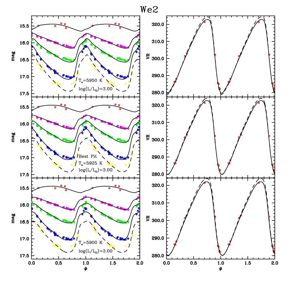
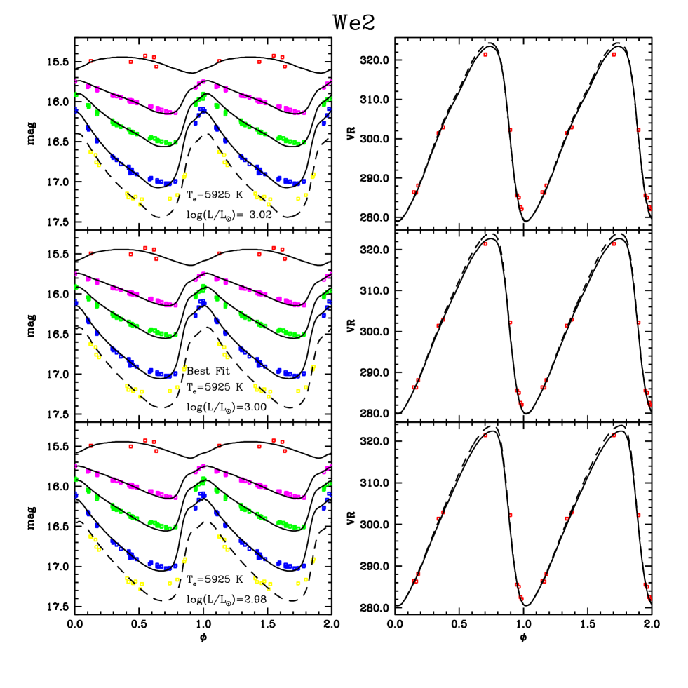
The best fit model selection illustrated above is shown for the fundamental pulsator We 2 in Figs.1-2. The best fit model (central panels in the two figures) has a characteristic effective temperature of 5925 K and a luminosity $\log(L/L_{\odot})=3.00$ dex. As evident in the top and bottom panels, a variation of 25 K in the temperature (at fixed luminosity) or 0.02 dex in the luminosity (at fixed temperature) worsen the match with the data. As mentioned above, we define the parameter uncertainty intervals as the half of the quoted variations. We also note that the chosen value of the projection factor p=1.27 provides an excellent match of the model radial velocity with the plotted data, even if the best analytic match is obtained for p=1.23.

Figure 1: In each one of the three panels on the left, the U, B, V, I and K band observed light curves of the Cepheid We 2 are shown from bottom to top (empty squares). The data have been systematically shifted to be shown in the same plot. The radial velocity data of the same star is shown in the three panels on the right (empty squares). The solid lines represent the model matched to the data. The U band model is plotted with dashed line because it will be excluded in our further analysis (see Sec.4.3). The best fit (BF) is plotted in the central panels and the models corresponding to $T_{e}^{BF}-2\delta T$ and $T_{e}^{BF}+2\delta T$, are shown in the bottom and top panels respectively. In the panels showing the radial velocity curves, the models with p-factor free to vary are also plotted (long dashed lines).

Figure 2: The same as Fig. 1 but with models corresponding to $\log(L/L_{\odot})^{BF}-2\delta(\log L/L_{\odot})$ and $\log(L/L_{\odot})+2\delta\log(L/L_{\odot})$, for We 2.

4.1.2 V6

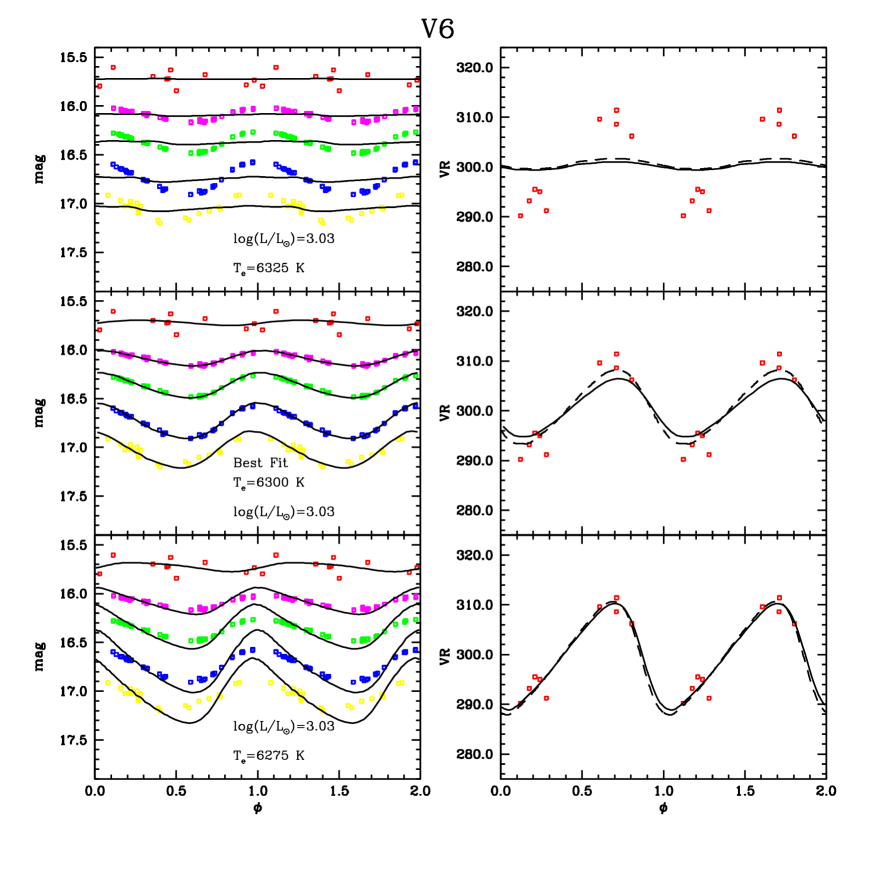
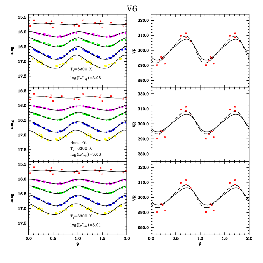
It is instructive to show the same plots than We 2 for the first overtone pulsator V6 (Figs.3-4). In this case we note that the best fit model is located very close to the first overtone blue edge, so that a shift of only $25K$ towards higher effective temperatures (see the top panel of Fig.3) almost quenches the pulsation. On the other hand when decreasing the effective temperature by $25K$ (bottom panel of the same figure), the predicted amplitudes increase significantly beyond the observed ones. If we consider the effect of a variation in the stellar mass we note that the corresponding variation in the pulsation amplitudes is much smaller, even if non negligible when computing the $\chi^{2}$ minimization.

The procedure of best fitting of the radial velocity curve, when considering the projection factor as a free parameter, provides the value p=1.00, which is significantly different from 1.27 and smaller than other typical values adopted in the literature. A possible explanation might be a not sufficiently good quality of the data, but we note that similar results have been discussed by Natale et al. (2008) for $\delta$ Cephei using a well sampled radial velocity curve.

Figure 3: The same as Fig. 1 for V6.

Figure 4: The same as Fig. 2 for V6.

4.1.3 HV 12197

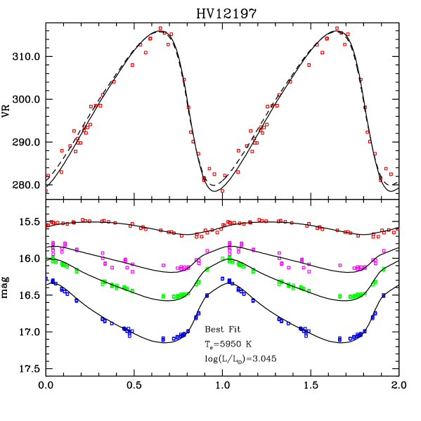
The two panels of Fig.5 show the best fitting result for Cepheid HV 12197. The U band is excluded from our analysis due to the poor light curve. According to the best fit model this star is the most luminous of our sample ($\log(L/L_{\odot})=3.045$ dex) and has an effective temperature of 5950 K. As for the radial velocity curve, the chosen value of the projection factor (1.27) provides a good match with the data and it is not significantly different from the value p=1.33 obtained from the $\chi^{2}$ minimization with variable p.

Figure 5: The best fit model light curves and the model radial velocity curves (solid lines) for the Cepheid HV 12197 are matched with the data (empty squares), in the bottom and top panel respectively. The plotted light curves are in the B, V, I and K bands from bottom to top. The best fit radial velocity curve obtained by varying the projection factor is shown as dashed line.

4.1.4 HV 12199

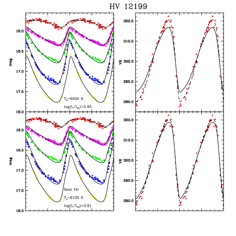
The best fit model for the Cepheid HV 12199 is shown in the bottom panels of Fig.6. The luminosity derived from the fitting procedure ($\log(L/L_{\odot})=2.91$ dex) results to be the smallest in the selected sample and the effective temperature of this star is 6125 K. The model radial velocity curve, plotted in the right panel, shows a small discrepancy in its amplitude with the data if we fix the value of the p factor to 1.27. It is necessary to decrease the projection factor to 1.17 in order to achieve the best match. It is interesting to note that, if we focus our attention only on the photometric data, the resulting best fit model for HV 12199 is given in the top panels of Fig.6, with a predicted effective temperature and $\log(L/L_{\odot})$ of 6200 K and 2.93 dex, respectively. However, we excluded this model because the radial velocity curve, obtained from the chosen value of the projection factor, has a too small amplitude to fit the data, (see the solid line in the Fig.6). To account for the amplitude of the radial velocity data it would be necessary to decrease the projection factor to the too small value p$\sim$1.0 (dashed line in the Figure). This inconsistency that can be indeed due to a too high model effective temperature, led us to prefer the best model reported in Fig.6

Figure 6: In the bottom panels the match between the best fit model and data, for the Cepheid HV 12199, is plotted with the same meaning of the used symbols than in the Fig.5. The plots in the top panels refer to a model with T=6200 K, $\log(L/L_{\odot})=2.93$ and $M/M_{\odot}=3.5$.

4.1.5 HV 12198

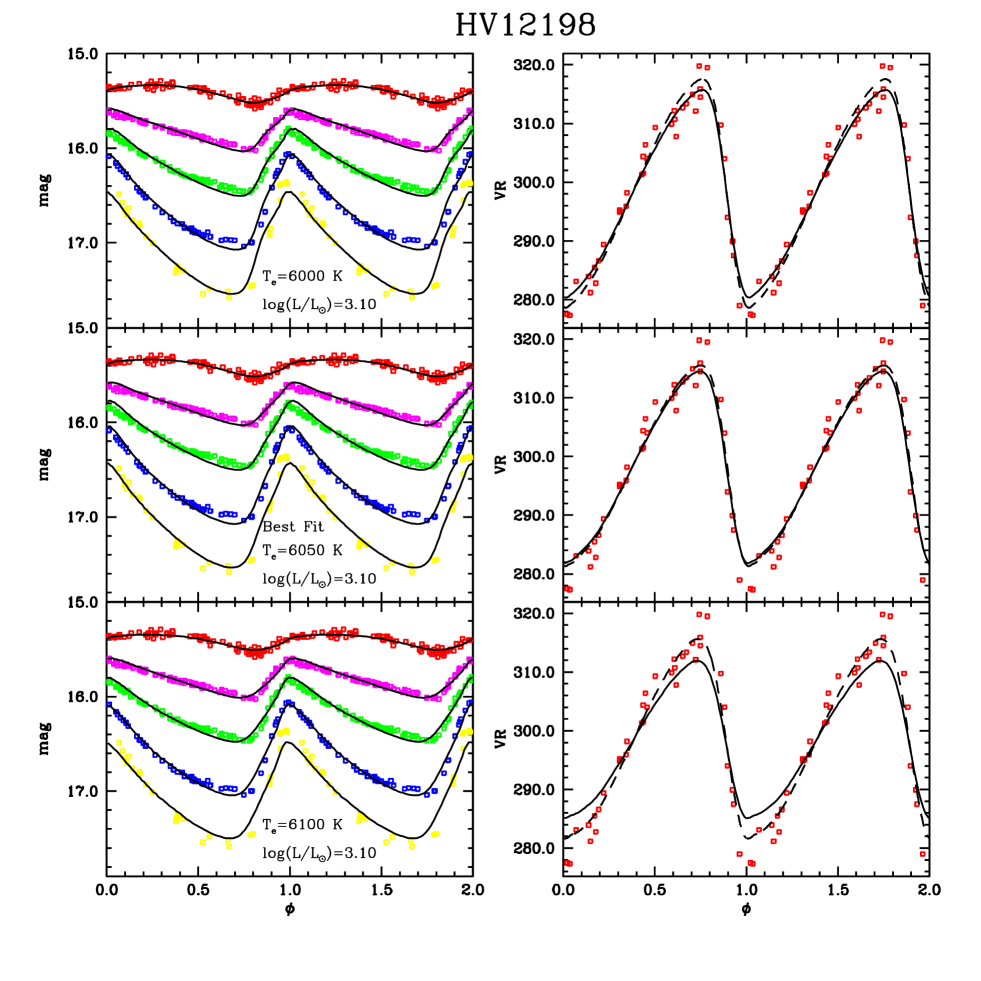
Fig.7 shows three possible models which describe the photometric and radial velocity data of HV 12198. The minimum $\chi^{2}$ for the photometry is obtained for the model at $T_{e}=6100$ K and $\log(L/L_{\odot})=3.10$ dex (bottom panel). However, this does not reproduce accurately the amplitude neither of the U band photometry nor of the radial velocity data. Decreasing the parameter of the convection efficiency, $\alpha_{ml}$, would produce the simultaneous increment of the amplitudes of both light and radial velocity curves. In this way we would recover the amplitudes of both the U band and the radial velocity curves, but we would decrease the accuracy of the fit in the remaining bands. As in the case of HV 12199, the radial velocity amplitude could be reproduced by decreasing the p factor to the barely acceptable value of $\sim 1$. If we exclude the U band, the model matching both the photometry and the radial velocity data is the one shown in the top panel of Fig.7, corresponding to $T_{e}$=6000 K and $\log(L/L_{\odot})=3.1$. In this case we obtain an accurate fit of the radial velocity data with the chosen projection factor value, which decreases to 1.15 if we consider it as a free parameter in the $\chi^{2}$ minimization. On the basis of these results, we decided to consider as our best fit model for HV 12198 an intermediate case between those already described. It is shown in the central panel, includes the U band fitting and provides a match of the radial velocity curve which is somewhat intermediate between those of the models in the top and bottom panels.

Figure 7: The match between model curves and data is shown for the best fit (central panel) and other two possible models, characterized by the same luminosity of the best fit one but slightly lower ($T_{e}$=6000 K top panels) and higher ($T_{e}$=6100 K bottom panels) effective temperature. As in the previous figures, the photometry is modeled in the left panels and the radial velocity in the right ones. Moreover, the light curves in the U, B, V, I and K band are represented from the bottom to the top. In the radial velocity panels, the dashed lines represent the model radial velocity curves obtained from the fit with free p factor.

Table 2: In the top part of the table adopted structural parameters (with uncertainties) of the best fit models obtained for the chemical composition Z=0.008 and Y=0.25: (1) Cepheid name, (2-3) mass, (4-5) luminosity, (6) canonical luminosity, (7-8) temperature, (9-10) barycentric velocity, (11-12) p factor, (13) convection efficiency parameter. In the bottom part of the table the distance moduli (with uncertainties) for all the photometric band obtained from the fit: (1) Cepheid name, (2-3) U band, (4-5) B band, (6-7) V band, (8-9) I band, (10-11) K band.

Structural parameters
Name	$\frac{M}{~{}M_{\odot}}$	$\delta\left(\frac{M}{~{}M_{\odot}}\right)$	$\log\left(\frac{L}{~{}L_{\odot}}\right)$	$\delta\log\left(\frac{L}{~{}L_{\odot}}\right)$	$\log\left(\frac{L}{~{}L_{\odot}}\right)_{can}$	T(K)	$\delta$T	$\gamma$ (km/s)	$\delta\gamma$	p	$\delta$p	$\alpha_{ml}$
HV 12197	4.6	$\pm$0.2	3.045	$\pm$0.012	3.01	5950	$\pm$12	298.3	$\pm$0.9	1.330	${}^{+0.025}_{-0.003}$	2.0
HV 12198	4.2	$\pm$0.1	3.10	$\pm$0.01	2.88	6050	$\pm$12	298.57	$\pm$0.09	1.216	${}^{+0.002}_{-0.102}$	2.0
HV 12199	3.5	$\pm$0.1	2.91	$\pm$0.01	2.62	6125	$\pm$12	300.9	$\pm$1.0	1.17	${}^{+0.03}_{-0.04}$	2.0
We 2	4.30	$\pm$0.15	3.00	$\pm$0.01	2.92	5925	$\pm$12	302.6	$\pm$0.6	1.232	${}^{+0.006}_{-0.012}$	1.9
V 6	4.0	$\pm$0.1	3.03	$\pm$0.01	2.81	6300	$\pm$12	300.6	$\pm$1.0	1.00	:	1.8
Distance moduli (mag)
Name	$\mu_{U}$	$\delta\mu_{U}$	$\mu_{B}$	$\delta\mu_{B}$	$\mu_{V}$	$\delta\mu_{V}$	$\mu_{I}$	$\delta\mu_{I}$	$\mu_{K}$	$\delta\mu_{K}$
HV 12197	…	…	19.09	$\pm$0.04	18.96	$\pm$0.05	18.89	$\pm$0.06	18.68	$\pm$0.04
HV 12198	19.15	$\pm$0.08	19.13	$\pm$0.05	18.98	$\pm$0.05	18.81	$\pm$0.04	18.60	$\pm$0.03
HV 12199	18.97	$\pm$0.05	18.96	$\pm$0.07	18.83	$\pm$0.06	18.68	$\pm$0.04	18.49	$\pm$0.04
We 2	18.70	$\pm$0.08	18.82	$\pm$0.05	18.78	$\pm$0.04	18.71	$\pm$0.03	18.53	$\pm$0.06
V6	19.10	$\pm$0.04	19.19	$\pm$0.02	19.03	$\pm$0.02	18.87	$\pm$0.02	18.61	$\pm$0.07

4.2 Comparison with the spectroscopic data

As a test for the accuracy of our procedure, we compared the effective temperature predicted by the best fit models for HV 12197 and HV 12199, with the results obtained by Mucciarelli et al. (2011) using an independent spectroscopic determination. The two panels of Fig.8 show the model temperature as a function of the pulsational phase of the two quoted Cepheids and their spectroscopic temperatures, given by Mucciarelli et al. (2011) with a typical error bar of 100 K.

Figure 8: Effective temperature curves predicted by models (solid lines) with overplotted spectroscopic determinations by Mucciarelli et al. (2011) (empty squares) for HV 12197 and HV 12199 in the bottom and top panels respectively.

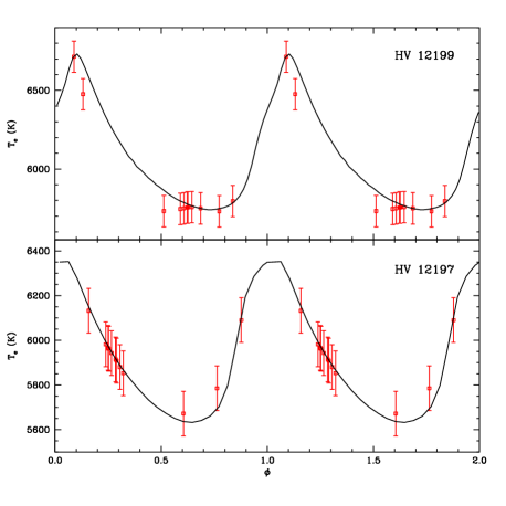
It is evident that models reproduce the spectroscopic data with great accuracy, thus further supporting the predictive capabilities of the adopted theoretical scenario, as well as of the model fitting technique.

4.3 Distance and reddening

Beyond the intrinsic stellar parameters of the best fit models (chemical composition, stellar mass, effective temperature, luminosity and convective efficiency parameter) and the corresponding projection factor, Tab.2 reports the resulting distance moduli in all the observed bands, $\mu_{i}$ (i=U, B, V, I, K), with the exception of HV 12197, for which the U band data consists only of three measurements and is not used to infer the distance. The range of values we find for the apparent distance moduli of the selected stars can be at least in part understood in terms of differential reddening, but other effects might in principle be at work (see below). Using the obatined apparent distance moduli and the photometric band effective wavelengths, $\lambda_{i}$, we fitted the Cardelli et al. (1989) extinction law to derive simultaneously the absorption, $A_{V}$, and the true distance modulus, $\mu_{0}$, for the selected Cepheids. To this aim, we minimized the following $\chi^{2}$ function by varying the two unknown parameters:

$$\chi^{2}=\sum^{N_{bands}}_{i=1}\left[\mu_{i}-\left(a(x_{i})+\frac{b(x_{i})}{R_{V}}\right)A_{V}-\mu_{0}\right]$$ (4)

where the total to selective extinction ratio is fixed to $R_{V}=3.3$ (Feast & Walker, 1987), $x_{i}\equiv\frac{1}{\lambda_{i}}$ is the inverse of the i band effective wavelength and the expressions for $a(x)$ and $b(x)$ are defined in Cardelli et al. (1989).

Figure 9: The result of the best fit of the Cardelli et al. (1989) reddening law is plotted for the five selected Cepheids (solid line). The data points (empty squares) represents the distance moduli obtained from the model fitting in the photometric bands considered in this work. The two filled triangles represent the U band distance moduli of V 6 and We 2 excluded from the fit.

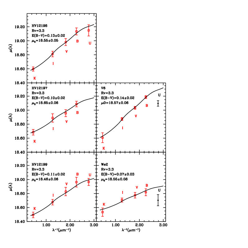
The results of the fit are shown in fig. 9 and the best fit parameters are listed in Tab. 3. To be conservative, the errors on the individual band distance moduli include the rms of the fitting procedure and the error related to the selection of the best fit model, summed in quadrature. Finally, the uncertainties on the parameters of the Cardelli fit have been derived from the $\chi^{2}$ confidence level at $1\sigma$. In the fitting procedure, we decided to exclude the U band distance moduli of We 2 and V 6 because they significantly deviate from the expected trend (see the filled triangles in fig.9).

Inspection of Tab. 3, suggests color excess estimates larger than the typically adopted value for NGC 1866, namely E(B-V)=0.06 mag (Storm et al., 2005; Molinaro et al., 2012, and references therein), with the exception of the result for We 2. In fact, the resulting weighted mean value is E(B-V)=0.11$\pm$0.01 mag, consistent with the result by Groenewegen & Salaris (2003), E(B-V)=0.12$\pm$0.02 mag, as based on the simultaneous fit of the NGC 1866 Cepheid Period–Luminosity relation, in the B, V and I photometric bands.

As for the distance modulus of NGC 1866, a weighted mean of the obtained results for the five stars, provides $\mu_{0}=18.56\pm 0.03$ mag. Here, the uncertainty is only statistical but we are aware that several systematic effects are at work when reproducing observing quantities with pulsation models. First, we have to consider the effect of the adopted physical assumptions, namely the equation of state and the opacity tables. Previous theoretical investigations (Petroni et al., 2003; Valle et al., 2009) show that the effect of varying these ingredients is marginal and dominated by the effect of the model spatial risolution. The latter affects the predicted pulsation amplitudes and in turn the intrinsic parameters of the obtained best fit models. In particular, increasing the adopted spatial resolution by 10 mesh zones can imply a variation of about 100 K in the predicted effective temperature and of few hundredths of dex in the predicted luminosity level. Another important source of uncertainty is the treatment of the pulsation and convection coupling. Even if we adopt a nonlinear nonlocal time-dependent treatment of convection (see Stellingwerf, 1982; Bono et al., 1999, for details), the equation system is closed by adopting a free parameter related to the mixing lenght. Variations of the mixing lenght affect the pulsation efficiency and amplitude. In particular, by varying the mixing lenght parameters by more than $\pm 0.05$ from the value reported in Tab.2, we are not able to reproduce the observed curves, with resulting changes in the predicted luminosity levels smaller than $\pm 0.03$ dex. Obviously, this is only the effect of varyingh the mixing lenght parameter, but within the same turbulent convective model. Assuming a different treatment of convection might in principle produce larger errors even if we consider quite encouraging that the application of the model fitting technique, from different groups (e.g. Bono et al., 2002; Keller & Wood, 2002; Marconi & Clementini, 2005; Keller & Wood, 2006; McNamara et al., 2007) and using different approaches to the treatment of the pulsation-convection coupling, gives consistent results for the LMC distance modulus (Marconi & Clementini, 2005; Marconi, 2009). Finally, for what concern the light curves we have to consider the uncertainty on the adopted model atmosphere in transforming bolometric into B,V,I,K variations. According to our previous experience we know that theoretical predictions are dependent on the set of static atmosphere models adopted for transforming temperatures into colors. For example, changing the adopted model atmospheres from Castelli et al. (1997a, b) to Kurucz (1993) produces colour effects of the order of 0.01 mag. In conclusion, to be conservative, we assume a systematic effect of $\pm$ 0.1 mag on the inferred distance modulus, as due to all the above mentioned theoretical uncertainties. On this basis our final estimate of NGC1866 distance modulus is $\mu_{0}=18.56\pm 0.03(stat)\pm 0.1(syst)$ mag.

This result is in agreement within the uncertainty interval with the value $18.51\pm 0.03$ mag, obtained by Molinaro et al. (2012) from the Baade–Wesselink method, using the same p factor adopted as reference value in this work. Their estimates of the distance to HV 12197, We 2 and HV 12198, are in excellent agreement with the values reported in Tab. 3. In particular, they found 18.63$\pm$0.12 mag, 18.54$\pm$0.09 mag and 18.59$\pm$0.08 mag for HV 12197, We 2 and HV 12198 respectively. For the remaining two stars, HV 12199 and V 6, they found 18.62$\pm$0.10 mag and 18.83$\pm$0.11 mag, respectively, both systematically longer than our estimates, although consistent with them within the errors. In a recent work, using the infrared surface brightness method, Storm et al. (2011) obtained the distance for a sample of Cepheids in the LMC, including HV 12197, HV 12199 and HV12198, and their final value (18.45 $\pm$ 0.04) is in agreement with our results within the errors. However, they used a period dependent p factor given by the equation $p=1.550(\pm 0.04)-0.186(\pm 0.06)\log P$. This is required to obtain distances to LMC Cepheids independent of their pulsation periods and distances to Galactic Cepheids in agreement with the HST parallaxes, with their surface brightness method (see Storm et al., 2011). As stated by the authors themeselves, this relation is not easily reconciled with recent theoretical work (e.g. Nardetto et al. 2009) and provides p-factor values for short-period Cepheids (not less than 1.4), significantly larger than the results derived in the present study. This discrepancy could be due, at least in part, to limitations of our treatment of the coupling between pulsation and convection (see discussion above) but we have to note that the debate on the p factor and on its possible dependence on the pulsation period is still open in the recent literature (see e.g. Ngeow et al., 2012, and references therein).

Table 3: Parameters obtained by fitting Cardelli extinction law: the Cepheids are listed in the first column, the second and third columns contain, respectively, the extinction, $A_{V}$, and the reddening, $E(B-V)$, the intrinsic distance modulus, $\mu_{0}$ is in the last column.

Name	$A_{V}$ (mag)	E(B-V) (mag)	$\mu_{0}$ (mag)
HV 12197	$0.33\pm 0.07$	$0.10\pm 0.02$	$18.65\pm 0.06$
HV 12198	$0.43\pm 0.07$	$0.13\pm 0.02$	$18.55\pm 0.05$
HV 12199	$0.37\pm 0.07$	$0.11\pm 0.02$	$18.46\pm 0.06$
We 2	$0.23\pm 0.10$	$0.07\pm 0.03$	$18.55\pm 0.08$
V 6	$0.46\pm 0.07$	$0.14\pm 0.02$	$18.57\pm 0.06$

4.4 Mass–Luminosity relation

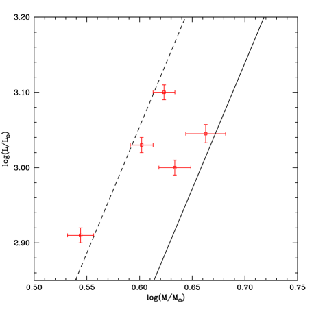
The obtained stellar masses for the Cepheids in NGC 1866, as reported in Tab.2, cover a range of values that might be the signature of differential mass loss. This occurrence is in agreement with previous findings by Brocato et al. (2004). Finally, we compared the derived masses and luminosities, as reported in Tab.2, with an evolutionary Mass–Luminosity relation (MLR) (Bono et al., 2000b), either neglecting or including mild overshooting according to the prescriptions by Chiosi et al. (1993).

Fig.10 clearly shows that the analyzed Cepheids do not follow one of the two relations, but they are randomly placed at intermediate luminosities between those predicted by the canonical and the mild overshooting MLRs, with the exception of the HV 12199 which results to be slightly more luminous than the mild overshooting prediction, although consistent with it within the uncertainties.

The fact that different luminosities are predicted for a given mass might suggest that the investigated Cepheid do not follow a MLR but are instead stochastically affected by some noncanonical phenomenon, likely a combination of mild overshooting and mass loss. However the application of the method to a larger sample of pulsators is needed in order to draw any reliable conclusion on the cause of the overluminosity distribution with respect to the canonical one.

Figure 10: The masses and luminosities of the analyzed Cepheids (empty squares) are compared with the canonical Mass–Luminosity relation (solid line) and with the mild overshooting Mass–Luminosity relation (dashed line).

5 Conclusions

We have used nonlinear convective pulsation models computed by our team to reproduce the multifilter (U,B,V, I and K) light and radial velocity curves of five Classical Cepheids in NGC 1866, a young massive cluster of the Large Magellanic Cloud. The resulting best fit models give us information on the intrinsic stellar parameters and the individual distances of the investigated Cepheids. In the case of HV 12197 and HV 12199 the obtained effective temperature and its variation with the pulsation phase has been found to be in very good agreement with the spectroscopic determinations within their uncertainties. The masses and luminosities, obtained for all the five investigated pulsators, from this model fitting technique satisfy a slightly brighter Mass–Luminosity relation than the canonical evolutionary one, indicating that noncanonical phenomena such as mild overshooting and/or mass loss are at work. As for the inferred distances, the individual values have been found to be consistent with each other within the uncertainties. Moreover, their weighted mean value corresponds to a distance modulus of 18.56$\pm$0.03 (stat) $\pm$ 0.1 (syst) mag, in agreement with several independent results in the literature. In particular the obtained result for the distance to NGC1866 is in excellent agreement with the results obtained from the application of the model fitting technique to LMC field Cepheids, RR Lyrae and $\delta$ Scuti variables (Bono et al., 2002; Marconi & Clementini, 2005; McNamara et al., 2007).

6 Acknowledgments

This paper utilizes public domain data obtained by the MACHO Project, jointly funded by the US Department of Energy through the University of California, Lawrence Livermore National Laboratory under contract No. W-7405-Eng-48, by the National Science Foundation through the Center for Particle Astrophysics of the University of California under cooperative agreement AST-8809616, and by the Mount Stromlo and Siding Spring Observatory, part of the Australian National University. We thank an anonymous referee for helpful comments and suggestions.

References

- Arp & Thackeray (1967) Arp, H., & Thackeray, A. D. 1967, ApJ, 149, 73
- Barmina et al. (2002) Barmina, R., Girardi, L., & Chiosi, C. 2002, A&A, 385, 847
- Bessell & Brett (1988) Bessell, M.S. & Brett, J.M., 1988, PASP, 100, 1134
- Bono et al. (2000a) Bono, G., Castellani, V., & Marconi, M., 2000, ApJ, 529, 293
- Bono et al. (2000b) Bono, G., Caputo, F., Cassisi, S., et al. 2000, ApJ, 543, 955
- Bono et al. (2002) Bono, G., Castellani, V., & Marconi, M. 2002, ApJL, 565, L83
- Bono & Stellingwerf (1994) Bono, G., & Stellingwerf, R. F. 1994, ApJS, 93, 233
- Bono et al. (1999) Bono, G., Marconi, M., & Stellingwerf, R. F. 1999, ApJS, 122, 167
- Brocato et al. (1989) Brocato, E., Buonanno, R., Castellani, V., & Walker, A. R. 1989, ApJS, 71, 25
- Brocato et al. (1994) Brocato, E., Castellani, V., & Piersimoni, A. M. 1994, A&A, 290, 59
- Brocato et al. (2003) Brocato, E., Castellani, V., Di Carlo, E., Raimondo, G., & Walker, A. R. 2003, AJ, 125, 3111
- Brocato et al. (2004) Brocato, E., Caputo, F., Castellani, V., Marconi, M., & Musella, I. 2004, AJ, 128, 1597
- Buchler & Szabó (2007) Buchler, J. R., & Szabó, R. 2007, ApJ, 660, 723
- Cardelli et al. (1989) Cardelli, J.A., Clayton, G.C., & Mathis, J.S., 1989, ApJ, 345, 245
- Castelli et al. (1997a) Castelli, F., Gratton, R. G., & Kurucz, R. L. 1997a, A&A, 324, 432
- Castelli et al. (1997b) Castelli, F., Gratton, R. G., & Kurucz, R. L. 1997b, A&A, 318, 841
- Chiosi et al. (1989) Chiosi, C., Bertelli, G., Meylan, G., & Ortolani, S. 1989, A&A, 219, 167
- Chiosi et al. (1993) Chiosi, C., Wood, P.R., & Capitanio, N., 1993, ApJS, 86, 541
- Di Criscienzo et al. (2004) Di Criscienzo, M., Marconi, M., & Caputo, F. 2004, ApJ, 612, 1092
- Di Fabrizio et al. (2002) Di Fabrizio, L., Clementini, G., Marconi, M., et al. 2002, MNRAS, 336, 841
- Feast & Walker (1987) Feast, M.W. & Walker, A.R., 1987, ARA&A, 25, 345
- Feast & Catchpole (1997) Feast, M.W. &, Catchpole, R.M., 1997, MNRAS, 286, L1
- Feuchtinger (1999) Feuchtinger, M. U. 1999, A&AS, 136, 217
- Fiorentino et al. (2007) Fiorentino, G., Marconi, M., Musella, I., & Caputo, F. 2007, A&A, 476, 863
- Fischer et al. (1992) Fischer, P., Welch, D. L., Cote, P., Mateo, M., & Madore, B. F. 1992, AJ, 103, 857
- Freedman (1988) Freedman, W.L. 1988, ApJ, 326, 691
- Freedman et al. (2001) Freedman, W. L., Madore, B. F., Gibson, B. K., et al. 2001, ApJ, 553, 47
- Gieren et al. (1994) Gieren, W. P., Richtler, T., & Hilker, M. 1994, ApJL, 433, L73
- Gieren et al. (2000) Gieren, W.P., Gómez, M., Storm, J., et al., 2000, ApJS, 129, 111
- Groenewegen & Salaris (2003) Groenewegen, M.A.T., & Salaris, M., 2003, A&A, 410, 887
- Keller & Wood (2002) Keller, S. C., & Wood, P. R. 2002, Apj, 578, 144
- Keller & Wood (2006) Keller, S. C., & Wood, P. R. 2006, Apj, 642, 834
- Kurucz (1993) Kurucz, R. L. 1993, Physica Scripta Volume T, 47, 110
- Labhardt, Sandage & Tammann (1997) Labhardt, L., Sandage, A., Tammann, G.A., 1997, A&A, 322, 751
- Leavitt & Pickering (1912) Leavitt, H. S., & Pickering, E. C. 1912, Harvard College Observatory Circular, 173, 1
- Madore & Freedman (1991) Madore, B. F., & Freedman, W. L. 1991, PASP, 103, 933
- Marconi & Clementini (2005) Marconi, M., & Clementini, G. 2005, AJ, 129, 2257
- Marconi & Degl’Innocenti (2007) Marconi, M., & Degl’Innocenti, S. 2007, A&A, 474, 557
- Marconi (2009) Marconi, M. 2009, Mem. SAIt, 80, 141
- Marconi et al. (2010) Marconi, M., Musella, I., Fiorentino, G., et al. 2010, ApJ, 713, 615
- McNamara et al. (2007) McNamara, D. H., Clementini, G., & Marconi, M. 2007, AJ, 133, 2752
- Molinaro et al. (2012) Molinaro, R., et al., 2012, ApJ, 748, 69
- Mucciarelli et al. (2011) Mucciarelli, A., Cristallo, S., Brocato, E., et al., 2011, MNRAS, 413, 837
- Musella et al. (2006) Musella, I., et al., 2006, Mem. SAIT, 77, 291
- Nardetto et al. (2009) Nardetto, N., Gieren, W., Kervella, P., et al., 2009, A&A, 502, 951
- Natale et al. (2008) Natale, G., Marconi, M., & Bono, G., 2008, ApJL, 674, L93
- Ngeow et al. (2012) Ngeow, C.-C., Neilson, H. R., Nardetto, N., & Marengo, M. 2012, A&A, 543, A55
- Olivier & Wood (2005) Olivier, E. A., & Wood, P. R. 2005, MNRAS, 362, 1396
- Petroni et al. (2003) Petroni, S., Bono, G., Marconi, M., & Stellingwerf, R. F. 2003, ApJ, 599, 522
- Riess et al. (2011) Riess, A. G., Macri, L., Casertano, S., et al. 2011, ApJ, 730, 119
- Riess et al. (2012) Riess, A. G., Macri, L., Casertano, S., et al. 2012, ApJ, 752, 76
- Robertson (1974) Robertson, J. W. 1974, ApJ, 191, 67
- Saha et al. (2001) Saha, A., Sandage, A., Tammann, G. A., et al. 2001, ApJ, 562, 314
- Stellingwerf (1982) Stellingwerf, R. F. 1982, ApJ, 262, 330
- Storm et al. (2004) Storm, J., et al, 2004, A&A, 415, 521
- Storm et al. (2005) Storm, J., Gieren, W.P., Fouqué, P., Barnes III, T.G. & Gómez, M., 2005, A&A, 440, 487
- Storm et al. (2011) Storm, J., Gieren, W., Fouqué, P., et al., 2011, A&A, 534, A95
- Storm et al. (2011) Storm, J., Gieren, W., Fouqué, P., et al. 2011, A&A, 534, A95
- Tammann & Reindl (2012) Tammann, G. A., & Reindl, B. 2012, ApSS, 43
- Testa et al. (1999) Testa, V., Ferraro, F. R., Chieffi, A., et al. 1999, AJ, 118, 2839
- Testa et al. (2007) Testa, V., et al., 2007, A&A, 462, 599
- Udalski et al. (1999) Udalski, A., Soszynski, I., Szymanski, M., et al. 1999, ActaA, 49, 223
- Valle et al. (2009) Valle, G., Marconi, M., Degl’Innocenti, S., & Prada Moroni, P. G. 2009, A&A, 507, 1541
- Walker (1995) Walker, A. R. 1995, AJ, 110, 638
- Walker et al. (2001) Walker, A. R., Raimondo, G., Di Carlo, E., et al. 2001, ApJL, 560, L139
- Wood et al. (1997) Wood, P. R., Arnold, A., & Sebo, K. M. 1997, ApJL, 485, L25
- Walker (2011) Walker, A. R. 2011, ApSS, 746
- Welch et al. (1991) Welch, D.L., Mateo, M., Côté, P., Fischer, P. & Madore, B.F., 1991, AJ, 101, 490
- Welch & Stetson (1993) Welch, D. L., & Stetson, P. B. 1993, AJ, 105, 1813