Absolute Properties of An Overcontact Binary HH Boo

Abstract

We obtained multi-colour light curves of HH Boo. We analysed the orbital period variation of the system. The analysis indicated that there is possible mass transfer from the second component to the primary or mass loss with $-5.04\times 10^{-7}$ $M_{\odot}$ per year. Re-analysing the available radial velocity curve, we analysed the light curves. The inclination ($i$) of the system was found to be 69^∘.71$\pm$0^∘.16, while the semi-major axis ($a$) was computed as 2.246$\pm$0.064 $R_{\odot}$. The mass of the primary component was found to be 0.92$\pm$0.08 $M_{\odot}$, while it was obtained as 0.58$\pm$0.06 $M_{\odot}$ for the secondary component. The radius of the primary component was computed as 0.98$\pm$0.03 $R_{\odot}$, while it was computed as 0.80$\pm$0.02 $R_{\odot}$ for the secondary component. We demonstrated that HH Boo should be a member of the A-type subclass of W UMa binaries.

1 Introduction

HH Boo (GSC 03472-00641) is classified as an eclipsing binary of W UMa type (a contact binary) in the SIMBAD Database. For the first time, the system was listed in the TYCHO-2 Catalogue by Høg et al. (2000), who gave $V=11^{m}.32$ and $(B-V)=0^{m}.45$ for the system. Its variability nature was found by Maciejewski et al. (2003), who obtained the first light curve and gave the light elements as following: $T_{0}=2452764.50965$ and $P=0^{d}.318618$. Considering the spectra of the system, Maciejewski et al. (2003) indicated that the system should be from the spectral type G5III. Then, Maciejewski & Ligeza (2004) obtained the radial velocity curve of the system. They found that mass ratio is 0.633$\pm$0.042, while $M_{1}sin^{3}i=0.78\pm 0.08$ $M_{\odot}$ and $M_{2}sin^{3}i=0.49\pm 0.05$ $M_{\odot}$. Although Maciejewski et al. (2003) have obtained a light curve, there is no light curve analysis given in the literature. However, many minima times have been obtained along the years. Most of them are listed in the modern database of O-C Gateway (Paschke & Brát, 2006), while some others are given by Maciejewski & Karska (2004), Maciejewski & Niedzielski (2004), Brát et al. (2008), Hubscher et al. (2009), Hubscher et al. (2010), Walter (2010).

According to Ammons et al. (2006), who determined new temperatures and metallicities for more than 100,000 FGK dwarfs, the temperature of the system is 5699 K, while $[Fe/H]$ was found to be -0.57. The distance is 54 pc.

In the literature, there are several systems similar to HH Boo (Essam et al., 2010). In this study, we obtained multi-colour light curves. Analysing the orbital period variation, we adjusted the light elements of the system and derived the mass transfer rate between the components. Then, re-analysing the radial velocity obtained by Maciejewski & Ligeza (2004), we analysed the multi-colour light curve using the parameters such as mass ratio and semi-major axis.

2 Observations

Observations of the system were acquired with a thermoelectrically cooled ALTA $U+47$ 1024$\times$1024 pixel CCD camera attached to a 35 cm - Schmidt - Cassegrains - type MEADE telescope at Ege University Observatory. The observations were continued in BVR bands in the observing season 2011. Some basic parameters of program stars are listed in Table 1, in which the brightness and colours were taken from the General Catalogue of Variable Stars (Kholopov et al., 1988).

Although the program and comparison stars are very close on the sky, differential atmospheric extinction corrections were applied. The atmospheric extinction coefficients were obtained from observations of the comparison stars on each night. Heliocentric corrections were also applied to the times of the observations. The mean averages of the standard deviations are 0^m.023, 0^m.011, and 0^m.010 for observations acquired in the BVR bands, respectively. To compute the standard deviations of observations, we used the standard deviations of the reduced differential magnitudes in the sense comparisons (GSC 03472-00043) minus check (GSC 03472-01201) stars for each night. There was no variation observed in the standard brightness comparison stars.

3 Analysis of Orbital Period Variation

There are several minima times of the system in the literature (Paschke & Brát, 2006; Hubscher et al., 2010). In the analysis, we used nor visual observations neither the minima times with large error. We also obtained new 15 minima times. All the minima times used in this study are listed in Table 2. The standard deviation of each one obtained in this study is given in the brackets near its related digits in Table 2.

Using the regression calculation, investigations demonstrated that the main variation could be described by a downward parabolic curve, which must be caused by possible mass transfer from the second component to the primary or mass loss. Therefore, the main period variation was represented by the quadratic light elements, which are given by Equation (1).

$$Min~{}I~{}(Hel.)~{}=~{}24~{}54912.3236(2)~{}+~{}0^{d}.318666(1)~{}\times~{}E-1.3349(1)\times 10^{-11}~{}\times~{}E^{2}$$ (1)

where the standard deviations of each coefficient and each constant are given in the brackets near their related digits.

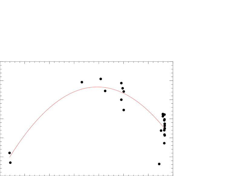
Figure 1: The O-C variation of HH Boo.

The period variation and its quadratic fit are shown in Figure 1. In the analyses, the weighted sum of the squared residuals, $\Sigma w(O-C)^{2}$, was found to be 0.000038 $day^{2}$. Considering the quadratic term ($Q$), the parameter of the period variation ($dP/dt$) was found to be -9.60$\times 10^{-7}$ $yr^{-1}$. The relation between the parameter of the period variation ($dP/dt$) and the rate of mass transfer was determined with Equation (2) by Pringle & Wade (1985):

$$\dot{m}~{}=~{}\frac{1}{3}~{}\times~{}\frac{M_{1}~{}\times~{}M_{2}}{M_{1}~{}-~{}M_{2}}~{}\times~{}\frac{\dot{P}}{P}$$ (2)

where $\dot{m}$ is mass transfer rate per year. Using this equation, the mass transferring from the secondary component to the primary was found to be $-5.04\times 10^{-7}$ $M_{\odot}~{}yr^{-1}$.

4 Radial Velocity and Light Curve Analyses

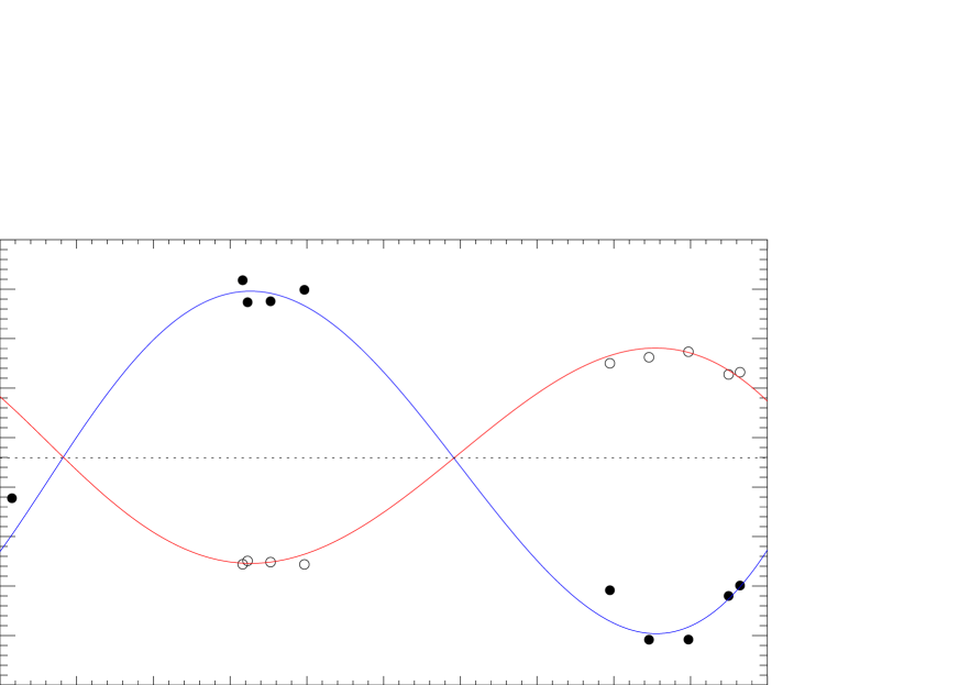
Figure 2: Radial velocity curve of HH Boo. Open circles represent the observations of the primary, while filled circles represent the secondary components. Solid curves are the theoretical radial velocity curves derived by the Spectroscopic Binary Solver software.

We took the radial velocity curve of the system from Maciejewski & Ligeza (2004). In order to adjust their radial velocity solution, we used the Spectroscopic Binary Solver software (Johnson, 2004) and re-analysed the radial velocity curve. In the analysis, we used the orbital period adjusted by the $O-C$ analyses in this study, and we fixed it. The results are listed in Table 3. The solution generally gave the same values obtained by Maciejewski & Ligeza (2004) with the little differences. The theoretical radial velocity curves derived by the Spectroscopic Binary Solver software are shown in Figure 2.

HH Boo is classified as an eclipsing binary of W UMa type in the SIMBAD Database, and it is more likely a contact binary system. In this respect, we analysed the light curves obtained in the BVR bands with using the PHOEBE V.0.31a software (Prša & Zwitter, 2005), which is used in the version 2003 of the Wilson-Devinney Code (Wilson & Devinney, 1971; Wilson, 1990). We tried to analyse the light curves with different modes, such as the ”overcontact binary not in thermal contact”, ”semi-detached system with the primary component filling its Roche-Lobe”, and ”double contact binary” modes. The initial analyses demonstrated that an astrophysical acceptable result can be obtained if the analysis is carried out in the ”overcontact binary not in thermal contact” mode, while no acceptable results in the astrophysical sense could be statistically obtained in all the others modes.

According to the radial velocity analysis, the mass ratio of the system should be 0.632$\pm$0.038. Ammons et al. (2006) determined the temperature of the system as 5699 K. Thus, the temperature of the primary component was fixed to 5699 K in the analyses, and the temperature of the secondary was taken as a free parameter. Considering the spectral type corresponding to this temperature, the albedos ($A_{1}$ and $A_{2}$) and the gravity darkening coefficients ($g_{1}$ and $g_{2}$) of the components were adopted for the stars with the convective envelopes (Lucy, 1967; Rucinski, 1969). The non-linear limb-darkening coefficients ($x_{1}$ and $x_{2}$) of the components were taken from Van Hamme (1993). In the analyses, the fractional luminosity ($L_{1}$) of the primary component and the inclination ($i$) of the system were also taken as the adjustable free parameters.

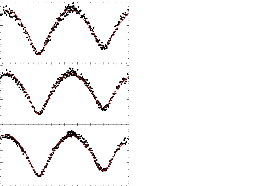
Figure 3: The BVR light curves of HH Boo and the synthetic solutions for the observations in each band.

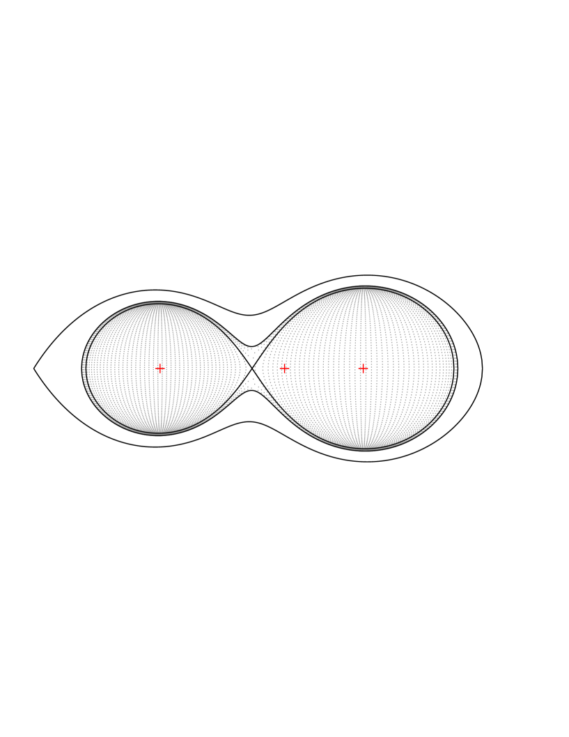
Figure 4: The Roche geometry of HH Boo.

The parameters derived from the analyses are listed in Table 4, while the synthetic light curves are shown in Figure 3. In addition, using the parameters obtained from the light curve analysis, we also derived the Roche geometry of the system that is shown in Figure 4.

Using the radial velocity curves, the mass ratio of the system ($q$) was obtained as 0.632$\pm$0.038, and the semi-major axis ($a$) was found to be 2.246$\pm$0.064 $R_{\odot}$. Considering both the radial velocity curve solution and the inclination ($i$) of the system found from the light curve analysis, the masses were found to be 0.92$\pm$0.08 $M_{\odot}$ for the primary component and 0.58$\pm$0.06 $M_{\odot}$ for the secondary component. Considering the semi-major axis, the radius of the primary component was computed as 0.98$\pm$0.03 $R_{\odot}$, while it was computed as 0.80$\pm$0.02 $R_{\odot}$ for the secondary component. In addition, the luminosity of the primary component was computed as 0.91$\pm$0.08 $L_{\odot}$, and it was computed as 0.47$\pm$0.03 $L_{\odot}$ for the secondary component.

In order to test whether the absolute parameters are generally acceptable in the astrophysical sense, or not, we compared the components with other systems in the mass-radius ($M-R$), mass-luminosity ($M-L$), and luminosity-effective temperature ($T_{eff}-L$) planes. All the comparisons are shown in Figure 5. In the figure, the lines represent the ZAMS theoretical model developed for the stars with $Z=0.02$ by Girardi et al. (2000), while dashed lines represent the TAMS theoretical model. The filled circles represent the primary components, while the open circles represents the secondary ones. The components of HH Boo are located together with some samples of its analogues, such as YY CrB, DN Boo, CK Boo, $\epsilon$ CrA, FG Hya, TV Mus, AW UMa, GR Vir, V776 Cas. The sample systems were taken from Essam et al. (2010), and they are shown in purple colour, while HH Boo is shown in black colour in Figure 5.

5 Discussion

In this study, we tried to determine the nature of an eclipsing binary system HH Boo. The analysis of orbital period variation indicates possible mass transfer from the second component to the primary and/or possible mass loss from the system. The size of transferring or loosing mass was computed as $-5.04\times 10^{-7}$ $M_{\odot}$ per year, which causes a decreasing in the orbital period due to the angular momentum loss. In fact, the parameter of the period variation was found to be -9.60$\times 10^{-7}$ $yr^{-1}$. We adjusted the orbital period as $0^{d}.318666$. It is well known that several binaries of W UMa type such as YY CrB (Essam et al., 2010), BS Cas (Yang et al., 2008), VZ Tri (Yang, 2010), exhibit large the period variation due to the large mass transfer.

We also re-analysed available radial velocity curve. Our solution seems to be a little bit different according to the results found by Maciejewski & Ligeza (2004). The differences should be caused due to the orbital period used in this study. Here, the adjusted period is a bit different from the one used by Maciejewski & Ligeza (2004).

For the first time in the literature, we analysed light curves of the system. The inclination ($i$) of the system was found to be 69^∘.71$\pm$0^∘.16, while the temperature of the secondary component was found to be 5352$\pm$15 K from the analysis. The fractional radii were found to be $r_{1}=0.435\pm 0.001$ for the primary component and $r_{2}=0.354\pm 0.001$ for the secondary one. In this case, the sum of fractional radii was computed as $r_{1}+r_{2}\simeq 0.80$. Thus, HH Boo seems to be in agreement with Kopal (1956)’s criteria for overcontact systems. The $O-C$ analysis indicates that the orbital period as $0^{d}.318666$. In addition, the temperature of the primary component is 5699 K, while the secondary one is 5352 K. Although some W UMa type binaries have components with some different surface temperature, they generally have the same surface temperature. Here, the primary component of HH Boo is a little bit hotter than the secondary one. The $O-C$ analysis indicates possible mass transfer from the second component to the primary. This case should be the reason of the hotter primary component. Considering some characteristics of the system such as the short orbital period, small mass ratio, hotter primary component and ect., HH Boo seems to be in agreement with the members of the A-type subclass of W UMa binaries (Berdyugina, 2005; Rucinski, 1985).

As it is seen from Figure 5, comparing HH Boo with its analogues in some planes, such as $M-R$, $M-L$, and $T_{eff}-L$ planes, demonstrated that the components of the system are in agreement with their analogues. On the other hand, both components are seen closer to each other in the figures. If the result obtained from the $O-C$ analysis is taken into account, it is possible that the secondary component will continue to lose its mass, while the primary will collect. Therefore, both components will have been separated from each other in the planes shown in Figure 5. However, they will get closer to each other in their orbits as it is in the models of Rocha-Pinto et al. (2002).

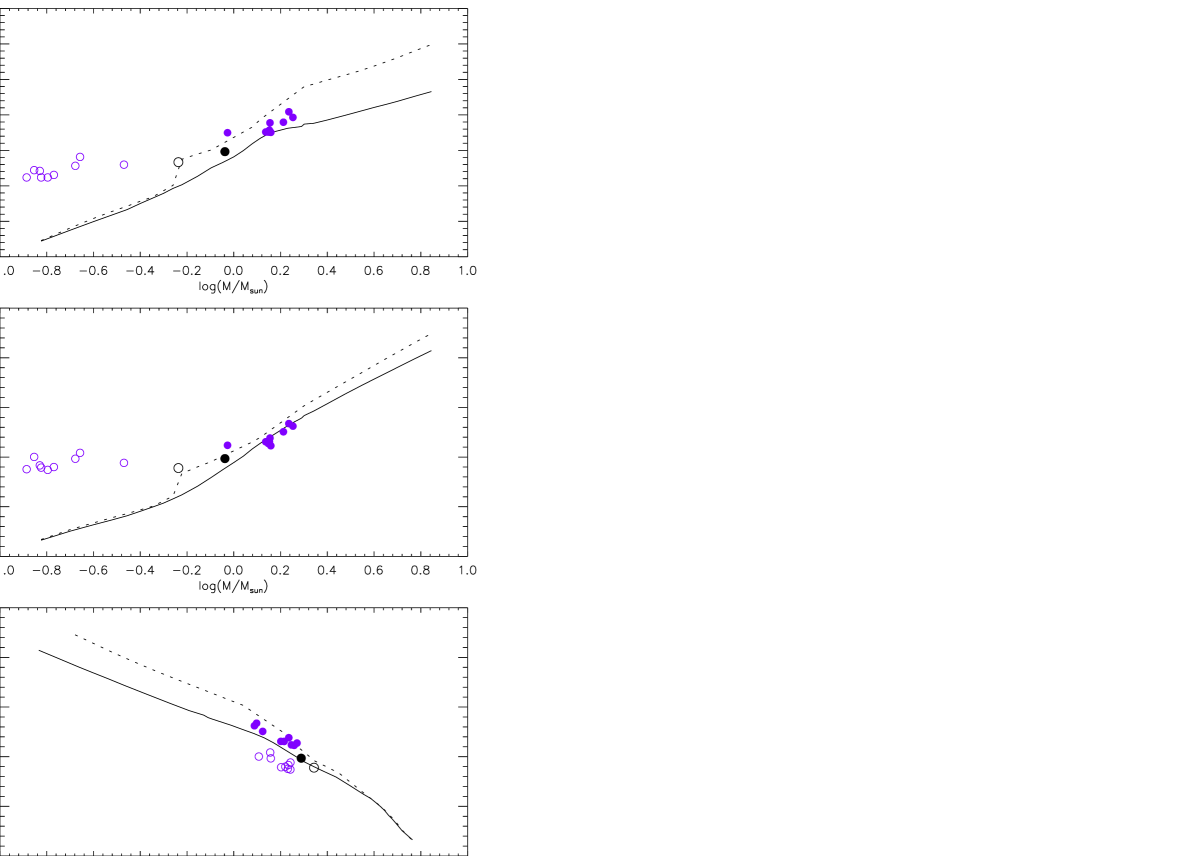
Figure 5: The places of the components of HH Boo in the planes of (upper panel) the mass-radius ($M-R$), (middle panel) mass-luminosity ($M-L$), and (bottom panel) luminosity-effective temperature ($T_{eff}-L$). In the panels, the continuous and dashed lines represent the ZAMS and TAMS theoretical models developed by Girardi et al. (2000), respectively. The filled circles represent the primary components, while the open circles represent the secondary ones. The dark circles represent the HH Boo components, while the purple coloured circles represent the components of other contact binaries.

Table 1: Basic parameters for the observed stars.

Star	Alpha (J2000)	Delta (J2000)	V	B-V
	(h m s)	(∘ ′ ′′)	(mag)	(mag)
HH Boo	14 21 44.06	46 41 59.40	11.272	0.654
GSC 03472-00043	14 21 46.59	46 43 49.40	12.906	0.595
GSC 03472-01201	14 21 37.30	46 46 18.90	13.701	0.662

Table 2: The minima times and ($O-C$) residuals (In the first column, the standard deviations of obtained minima times are given in the brackets near themselves).

O	E	$(O-C)_{II}$	Type	Method	REF
52749.5328	-9420.0	-0.00179	I	V	Paschke & Brát (2006)
52764.5096	-9373.0	-0.00230	I	V	Paschke & Brát (2006)
54148.6406	-5029.5	0.00192	II	Ir	Paschke & Brát (2006)
54513.5136	-3884.5	0.00209	II	Ir	Hubscher et al. (2010)
54599.3935	-3615.0	0.00146	I	CCD+R	Paschke & Brát (2006)
54912.3233	-2633.0	0.00100	I	Ir	Paschke & Brát (2006)
54912.4835	-2632.5	0.00187	II	Ir	Paschke & Brát (2006)
54937.3392	-2554.5	0.00160	II	Ir	Paschke & Brát (2006)
54958.6887	-2487.5	0.00046	II	V	Paschke & Brát (2006)
54958.8490	-2487.0	0.00143	I	V	Paschke & Brát (2006)
55644.9336	-334.0	-0.00237	I	V	Paschke & Brát (2006)
55680.7853	-221.5	-0.00062	II	V	Paschke & Brát (2006)
55716.4767(3)	-109.5	0.00013	II	R	This Study
55716.4768(5)	-109.5	0.00023	II	B	This Study
55716.4768(2)	-109.5	0.00025	II	V	This Study
55743.4026(3)	-25.0	-0.00128	I	R	This Study
55743.4032(4)	-25.0	-0.00060	I	V	This Study
55743.4038(2)	-25.0	-0.00008	I	B	This Study
55747.3863(5)	-12.5	-0.00083	II	R	This Study
55747.3871(3)	-12.5	-0.00003	II	V	This Study
55747.3874(4)	-12.5	0.00022	II	B	This Study
55751.3696(3)	0.0	-0.00087	I	V	This Study
55751.3700(3)	0.0	-0.00051	I	R	This Study
55751.3700(6)	0.0	-0.00050	I	B	This Study
55751.3701(2)	0.0	-0.00037	I	R	This Study
55751.3702(3)	0.0	-0.00027	I	V	This Study
55751.3702(4)	0.0	-0.00026	I	B	This Study

Table 3: The results of the analysis of Radial Velocity curve.

Parameter	Value	Error
Long. of Periastron1 (∘)	238.669	${}^{+49.884}_{-72.41}$
Long. of Periastron2 (∘)	58.669	${}^{+49.884}_{-72.41}$
Eccentricity ($e$)	0.048	${}^{+0.043}_{-0.042}$
Semi-Amplitude1 ($kms^{-1}$)	129.647	${}^{+6.4243}_{-6.2471}$
Semi-Amplitude2 ($kms^{-1}$)	205.078	${}^{+7.0675}_{-6.7157}$
Systemic Velocity ($kms^{-1}$)	2.9209	${}^{+4.0328}_{-4.0429}$
$a_{1}sini$ ($km$)	$5.67\times 10^{5}$	$\pm 3.68\times 10^{4}$
$a_{2}sini$ ($km$)	$8.98\times 10^{5}$	$\pm 4.86\times 10^{4}$
$m_{1}sin^{3}i$ ($M_{\odot}$)	$7.56\times 10^{-1}$	$\pm 9.99\times 10^{-2}$
$m_{2}sin^{3}i$ ($M_{\odot}$)	$4.78\times 10^{-1}$	$\pm 6.54\times 10^{-2}$

Table 4: The parameters of components obtained from the light curve analysis.

Parameter	Value
$i$ (∘)	69.71$\pm$0.16
$T_{1}$ (K)	5699
$T_{2}$ (K)	5352$\pm$15
$\Omega_{1}$	3.0492
$\Omega_{2}$	3.0402$\pm$0.0051
$L_{1}/L_{T}$ (B)	0.691$\pm$0.046
$L_{1}/L_{T}$ (V)	0.669$\pm$0.037
$L_{1}/L_{T}$ (R)	0.657$\pm$0.031
$g_{1}$, $g_{2}$	0.32, 0.32
$A_{1}$, $A_{2}$	0.50, 0.50
$x_{1,bol}$, $x_{2,bol}$	0.619, 0.619
$x_{1,B}$, $x_{2,B}$	0.765, 0.765
$x_{1,V}$, $x_{2,V}$	0.732, 0.732
$x_{1,R}$, $x_{2,R}$	0.655, 0.655
$<r_{1}>$	0.435$\pm$0.001
$<r_{2}>$	0.354$\pm$0.001

References

- Ammons et al. (2006) Ammons, S.M., Robinson, S.E., Strader, J., Laughlin, G., Fischer, D., Wolf, A., 2006, ApJ, 638, 1004
- Berdyugina (2005) Berdyugina, S.V., 2005, LRSP, 2, 8
- Brát et al. (2008) Brát, L., Šmelcer, L., Kuèáková, H., Ehrenberger, R., Kocián, R., Lomoz, F., Urbanèok, L., Svoboda, P., Trnka, J., Marek, P., and 5 coauthors, 2008, OEJV, 94, 1
- Essam et al. (2010) Essam, A., Saad, S.M., Nouh, M.I., Dumitrescu, A., El-Khateeb, M.M., Haroon, A., 2010, NewA, 15, 227
- Girardi et al. (2000) Girardi, L., Bressan, A., Bertelli, G., Chiosi, C., 2000, A&AS 141, 371
- Høg et al. (2000) Høg, E., Fabricius, C., Makarov, V.V., Urban, S., Corbin, T., Wycoff, G., Bastian, U., Schwekendiek, P., Wicenec, A., 2000, A&A, 355L, 27
- Hubscher et al. (2010) Hubscher, J., Lehmann, P.B., Monninger, G., Steinbach, H., Walter, F., 2010, IBVS, 5918, 1
- Hubscher et al. (2009) Hubscher, J., Steinbach, H.M., Walter, F., 2009, IBVS, 5874, 1
- Johnson (2004) Johnson, D.O., 2004, JAD, 10, 3
- Kholopov et al. (1988) Kholopov, P.N., Samus, N.N., Frolov, M.S., Goranskij, V.P., Gorynya, N.A., Karitskaya, E.A., Kazarovets, E.V., Kireeva, N.N., et al., 1985-1988, General Catalogue of Variable Stars, Vol. I III, 4th ed., Nauka, Moscow
- Kopal (1956) Kopal, Z., 1956. AnAp, 19, 298
- Lucy (1967) Lucy, L.B., 1967, Z. Astrophys, 65, 89
- Maciejewski et al. (2003) Maciejewski, G., Czart, K., Niedzielski, A., Karska, A., 2003, IBVS, 5431, 1
- Maciejewski & Karska (2004) Maciejewski, G., Karska, A., 2004, IBVS, 5494, 1
- Maciejewski & Ligeza (2004) Maciejewski, G., Ligeza, P., 2004, IBVS, 5504, 1
- Maciejewski & Niedzielski (2004) Maciejewski, G., Niedzielski, A., 2004, BaltA, 13, 700
- Paschke & Brát (2006) Paschke, A., Brát, L., 2006, OEJV, 23, 13
- Pringle & Wade (1985) Pringle, J.E. and Wade, R.A., 1985, ”Interacting Binary Stars”, Cambridge University Press., New York, p.17
- Prša & Zwitter (2005) Prša, A., Zwitter, T., 2005, ApJ, 628, 426
- Rocha-Pinto et al. (2002) Rocha-Pinto, H.J., Castilho, B.V., Maciel,W.J., 2002, A&A, 384, 912
- Rucinski (1969) Rucinski, S.M., 1969, AcA, 19, 245
- Rucinski (1985) Rucinski, S., 1985. In: Pringle, J.E., Wade, R.A. (Eds.), Interacting binary stars. Cambridge University Press, Cambridge. p. 1
- Yang et al. (2008) Yang, Y.-G., Wei, J.-Y., He, J.-J., 2008, AJ, 136, 594
- Yang (2010) Yang, Y.-G., 2010, Ap&SS, 326, 125
- Van Hamme (1993) Van Hamme, W., 1993, AJ, 106, 2096
- Walter (2010) Walter, F., 2010, BAVSR, 59, 139
- Wilson (1990) Wilson, R.E., 1990, ApJ, 356, 613
- Wilson & Devinney (1971) Wilson, R.E., Devinney, E.J., 1971, ApJ, 166, 605