Asymptotic controllability and optimal control

Abstract

We consider a control problem where the state must approach asymptotically a target ${\bf C}$ while paying an integral cost with a non-negative Lagrangian $l$. The dynamics $f$ is just continuous, and no assumptions are made on the zero level set of the Lagrangian $l$. Through an inequality involving a positive number $\bar{p}_{0}$ and a Minimum Restraint Function $U=U(x)$ –a special type of Control Lyapunov Function– we provide a condition implying that (i) the system is asymptotically controllable, and (ii) the value function is bounded by $U/\bar{p}_{0}$. The result has significant consequences for the uniqueness issue of the corresponding Hamilton-Jacobi equation. Furthermore it may be regarded as a first step in the direction of a feedback construction.

1 Introduction

Let ${\bf C}\subset{{{\rm I\mkern-3.5muR}}}^{n}$ be a closed subset, which will be called the target, and let ${\bf C}^{c}$ denote its complement. We consider the value function

$$\begin{array}[]{l}{{\mathcal{V}}}(x)\doteq{\inf}\,{\mathcal{J}}_{z,\alpha},\\ \\ \displaystyle{\mathcal{J}}_{z,\alpha}\doteq\int_{0}^{{T}_{z}}l(z(t),\alpha(t))\,dt\end{array}$$ (1)

for trajectory-control pairs $(z,\alpha):[0,{T}_{z}[:\to{\bf C}^{c}\times A$ subject to

$$\begin{array}[]{l}\dot{z}(t)=f(z(t),\alpha(t))\qquad z(0)=x\\ \\ \lim_{t\to{T}_{z}^{-}}{\bf d}(z(t),{\bf C})=0,\end{array}$$ (2)

where ${\bf d}$ denotes the Euclidean distance.

The crucial assumption of the paper will be the sign condition

$$l(x,a)\geq 0\qquad\forall(x,a)\in{\bf C}^{c}\times A.$$ (3)

In its stronger form, the main result of the paper (Theorem 1.1) reads as follows: Let $\bar{p}_{0}$ be a positive real number and let $U=U(x)$ be a proper, positive definite, semiconcave function such that, for every $x\in{\bf C}^{c}$, one has

$$H(x,\bar{p}_{0},D^{*}U(x))<0.\,\,\,\,$$ (4)

Then the system is globally asymptotically controllable and the value function ${{\mathcal{V}}}$ verifies the inequality

$${{\mathcal{V}}}(x)\leq U(x)/\bar{p}_{0},$$

for all $x\in{\bf C}^{c}$.

In (4), $H$ denotes the natural (minimized) Hamiltonian of the system, namely

$$H(x,p_{0},p)\doteq\inf_{a\in A}\left\langle(p_{0},p)\,,\,\Big{(}l(x,a),f(x,a)\Big{)}\right\rangle,\,\,\,\,\,$$ (5)

while $D^{*}$ is the generalized differential operator called limiting gradient (see Def. 1.4).

A function $U$ as above is here called a Minimum Restraint Function (Def. 1.1).

Let us make clear that condition (4) is not a mere application of the usual (first order) asymptotic global controllability condition to the enlarged dynamics obtained by adding the equation $\dot{z}_{0}=l(z,\alpha)$, with the enlarged target $[0,+\infty[\times{\bf C}$. Actually, the known conditions on the existence of a Control Lyapunov Function to characterize global asymptotic controllability would provide no information on the value of the minimum . Let us also anticipate that our result is valid under general hypotheses on $f$ and $l$ that do not guarantee neither uniqueness nor bounded length in finite time of the trajectories (see next subsection).

Investigations on this kind of value functions have been pursued in several papers, mainly from the point of view of the corresponding Hamilton-Jacobi equation. Indeed the existence of pairs $(x,a)$ such that $l(x,a)=0$ raises various non trivial problems about uniqueness. A likely incomplete bibliography, also containing applications (for instance, the Füller and shape-from-shading problems), includes [BCD], [I], [IR], [CSic], [Sor2], [M], [Ma], and the references therein.

Actually, besides displaying an obvious control theoretical meaning (see also Remark 1.4), our result provides a sufficient condition for the value function to be continuous on the target’s boundary. This continuity property is crucial to recover uniqueness of the corresponding boundary value problem (see Remark 1.3).

We conclude this informal presentation by observing that if some $\eta>0$ existed such that $l(x,a)\geq\eta$   $\forall(x,a)\in{{{\rm I\mkern-3.5muR}}}^{n}\times A$, then the problem could be easily reduced to an actual optimal time problem by just utilizing the reparameterized dynamics

$$\frac{dy}{d\tau}=\displaystyle\frac{f(y,\alpha)}{l(y,\alpha)}.$$

Indeed, after the (bi-Lipschitz) time-parameter change $\tau(t)\doteq\int_{0}^{t}l\,dt$ the Lagrangian turns out to be transformed into the constant value $1$. Yet, if only the weaker sign condition (3) is assumed, a direct approach based on such a reparameterization cannot be adopted.

The paper is organized as follows. In the remaining part of the present section we state rigorously the main result of the paper (Theorem 1.1) and provide some basic definitions. In Section 2 we sketch the main result’s proof by heuristic arguments and give a geometrical description of the thesis. Section 2 ends with some examples. Section 3 is the longest one, and is entirely devoted to the proof of Theorem 1.1, while some technical results are proved in Section 4. In Section 5 we make some remarks on the meaning of assumption (4) as a viscosity supersolution condition.

1.1 Precise statement of the main result

Our main technical assumptions are:

• for given positive integers $n$, $m$, the controls $\alpha(\cdot)$ take values in a compact set $A\subset{{{\rm I\mkern-3.5muR}}}^{m}$ and are Borel-measurable, while the state values $z(t)$, $x$ range over ${{{\rm I\mkern-3.5muR}}}^{n}$;

• the target ${\bf C}$ is closed and has compact boundary;

• the augmented vector field $(l,f)$ is a continuous function on ${\bf C}^{c}\times A$.

In particular, for any given control $\alpha(\cdot)$ and initial condition $z(0)=x$, the Cauchy problem associated to the differential equation (2) may have multiple Carathèodory solutions. Moreover, the latter may have unbounded velocity near ${\bf C}$, since $f$ itself is not assumed to be neither Lipschitz nor bounded near ${\bf C}$. Actually it may well happen that approaching trajectories fail to reach the target even when ${T}_{z}<+\infty$ (see Example 2.3).

Let us introduce the notion of Minimum Restraint Function.

Definition 1.1

We say that a continuous function $U:\overline{{\bf C}^{c}}\to{{{\rm I\mkern-3.5muR}}}$ is a Minimum Restraint Function, in short, a (MRF), if $U$ is locally semiconcave, positive definite, and proper on ${{\bf C}}^{c}$, and, moreover, there exists $\bar{p}_{0}\geq 0$ such that

$$H(x,\bar{p}_{0},D^{*}U(x))<0$$ (6)

holds true for all $x\in{\bf C}^{c}$.

Theorem 1.1

Let a Minimum Restraint Function $U$ exist. Then:

• the system (2) is globally asymptotically controllable to ${\bf C}$;

• if $U$ is a Minimum Restraint Function with $\bar{p}_{0}>0$, then

  $${{\mathcal{V}}}(x)\leq\frac{U(x)}{{{\bar{p}_{0}}}}\,\qquad\forall x\in{\bf C}^{c}.$$ (7)

Remark 1.1

Petrov-like inequalities (see Example 2.1) are included in condition (6). However, let us point out that they only concern the case where $l=1$ and the dynamics is bounded near the target, which implies that optimal (or quasi-optimal) trajectories take a finite time to reach the target. Instead when the Lagrangian is just non-negative, condition (6) does not force optimal trajectories to approach the target in finite time.

Remark 1.2

Because of the sign assumption (3), a Minimum Restraint Function, (MRF), is in particular a Control Lyapunov Function, (CLF). Hence, as a byproduct of statement (i) in Theorem 1.1 we get an extension to merely continuous, unbounded dynamics of the results concerning the relation between Control Lyapunov Functions and asymptotic controllability (see e.g. [S2]).

Remark 1.3

Because of the bound (7), the value function ${{\mathcal{V}}}$ turns out to be continuous on ${\partial\bf C}$. Actually, this is a theoretical motivation for a result like Theorem 1.1, in that the continuity of the value function on the target’s boundary is essential to establish comparison, uniqueness, and robustness properties for the associated Hamilton-Jacobi-Bellman equation (see [MS], [Sor1], and [M]).

Remark 1.4

Our investigation might be useful also for feedback control. Indeed, on the one hand the uniqueness of the H-J equation is an obvious ingredient in a feedback-oriented construction. On the other hand, a (MRF) $U$ can be possibly exploited in order to build a ”safe” feedback law for problem (1) (see e.g. [CLSS] and [AB] for general reference to feedback stabilization).

Remark 1.5

It is easy to adapt Theorem 1.1 to the case when the state space is an open set $\Omega\subset{{{\rm I\mkern-3.5muR}}}^{n}$, $\Omega\supset{\bf C}$. In fact, the thesis keeps unchanged as soon as one requires the (MRF) $U:\Omega\setminus\overset{\circ}{{\bf C}}\to{{{\rm I\mkern-3.5muR}}}$ to verify all the assumptions in Definition 1.1 in $\Omega$, plus the following one:

$$\exists U_{0}\in]0,+\infty]:\ \ \lim_{x\to x_{0},\ x\in\Omega}U(x)=U_{0}\ \ \forall x_{0}\in\partial\Omega;\quad U(x)<U_{0}\quad\forall x\in\Omega\setminus\overset{\circ}{{\bf C}}.$$

1.2 Basic definitions

For the reader convenience, some classical concepts, like (GAC), and a few technical definitions (part of which have already been used in Theorem 1.1 above) are here recalled.

Definition 1.2

(Positive definiteness). A continuous function $U:\overline{{\bf C}^{c}}\to{{{\rm I\mkern-3.5muR}}}$ is said positive definite on ${\bf C}^{c}$ if $U(x)>0$  $\forall x\in{{\bf C}}^{c}$ and $U(x)=0$  $\forall x\in\partial{\bf C}$. Moreover $U$ is called proper on ${{\bf C}}^{c}$ if $U^{-1}(K)$ is compact as soon as $K\subset[0,+\infty[$ is compact.

Definition 1.3

(Semiconcavity). Let $\Omega\subset{{{\rm I\mkern-3.5muR}}}^{n}$ be an open set, and let $F:\Omega\to{{{\rm I\mkern-3.5muR}}}$ be a continuous function. $F$is said to be locally semiconcave on $\Omega$ if for any point $x\in\Omega$ there exist $R>0$ and $\rho>0$ such that

$$F(z_{1})+F(z_{2})-2F\left(\frac{z_{1}+z_{2}}{2}\right)\leq R|z_{1}-z_{2}|^{2}\quad\forall z_{1},\,z_{2}\in B_{n}(x,\rho).$$

Let us remind that locally semiconcave functions are locally Lipschitz. Actually, they are twice differentiable almost everywhere (see e.g. [CS]).

Definition 1.4

(Limiting gradient). Let $\Omega\subset{{{\rm I\mkern-3.5muR}}}^{n}$ be an open set, and let $F:\Omega\to{{{\rm I\mkern-3.5muR}}}$ be a locally Lipschitz function. For every $x\in\Omega$ let us set

$$D^{*}{F}(x)\doteq\Big{\{}w\in{{{\rm I\mkern-3.5muR}}}^{n}:\ \ w=\lim_{k}\nabla{F}(x_{k}),\ \ x_{k}\in DIFF(F)\setminus\{x\},\ \ \lim_{k}x_{k}=x\Big{\}}$$

where $\nabla$ denotes the classical gradient operator and $DIFF(F)$ is the set of differentiability points of $F$. $D^{*}{F}(x)$ is called the set of limiting gradients of $F$ at $x$.

For every $x\in\Omega$, $D^{*}{F}(x)$ is a nonempty, compact subset of ${{{\rm I\mkern-3.5muR}}}^{n}$ (more precisely, of the cotangent space $T^{*}_{x}\Omega$). Notice that, in general, $D^{*}{F}(x)$ is not convex.

To give the notion of global asymptotic controllability we need to recall the concept of function belonging to ${\cal KL}$: these are continuous functions $\beta:[0,+\infty[\times[0,+\infty[\to[0,+\infty[$ such that: (1)  $\beta(0,t)=0$ and $\beta(\cdot,t)$ is strictly increasing and unbounded for each $t\geq 0$; (2)  $\beta(r,\cdot)$ is decreasing for each $r\geq 0$; (3)  $\beta(r,t)\to 0$ as $t\to+\infty$ for each $r\geq 0$. For brevity, let us use the notation ${\bf d}(x)$ in place of ${\bf d}(x,{\bf C})$.

Definition 1.5

(GAC) The system (2) is globally asymptotically controllable to ${\bf C}$ –shortly, (2) is (GAC) to ${\bf C}$– provided there is a function $\beta\in{\cal KL}$ such that, for each initial state $x\in{\bf C}^{c}$, there exists an admissible trajectory-control pair $(z,\alpha):[0,+\infty[\to{{{\rm I\mkern-3.5muR}}}^{n}\times A$ that verifies

$${\bf d}(z(t))\leq\beta({\bf d}(x),t)\qquad\forall t\in[0,+\infty[.$$ (8)

In Theorem 1.1’s proof we shall make use of the notions of partition of an interval and of its diameter. To avoid vagueness let us state the precise meaning we attach to these terms.

Definition 1.6

Let us consider an interval $[0,b[$,   $b\in]0,+\infty]$. A partition of $[0,b[$ is a sequence $\pi=(t^{j})$ such that $t^{0}=0,\quad t^{j-1}<t^{j}$   $\forall j\geq 1$, and either $\lim_{j\to+\infty}t^{j}=b$ or there exists some $n_{\pi}\in{{{\rm I\mkern-3.5muN}}}$ such that $t^{n_{\pi}}=b$. In the latter case, we say that $\pi$ is a finite partition of $[0,b[$. The number diam$(\pi)\doteq\sup_{\{j:\ t^{j}\leq b\}}(t^{j}-t^{j-1})$ is called the diameter of the sequence $\pi$.

2 Heuristics of the proof and some examples

2.1 A one dimensional differential inequality

As in the case of asymptotic controllability, the underlying idea of Theorem 1.1 relies on a one-dimensional argument involving a differential inequality. To express this issue, let us assume some simplifying facts. Let us begin with making the hypothesis that $U$ is of class $C^{1}$, so that assumption (6) reads

$$\inf_{a\in A}\left\langle(\bar{p}_{0},\nabla U(x))\,,\,\Big{(}l(x,a),f(x,a)\Big{)}\right\rangle<0\qquad\forall x\in{\bf C}^{c}.$$ (9)

Let us also assume that there exists a continuous selection

$$a(x)\in A(x)\doteq\left\{a\in A:\ \left\langle(\bar{p}_{0},\nabla U(x))\,,\,\Big{(}l(x,a),f(x,a)\Big{)}\right\rangle<0\right\},$$

so that (9) yields

$$\left\langle(\bar{p}_{0},\nabla U(x))\,,\,\Big{(}l(x,a(x)),f(x,a(x))\Big{)}\right\rangle<0\qquad\forall x\in{\bf C}^{c}$$ (10)

for some $\bar{p}_{0}\geq 0$.

Let us consider a solution of the augmented Cauchy problem

$$\left\{\begin{array}[]{l}\dot{z}_{0}=l(z,a(z))\\ \\ \dot{z}=f(z,a(z))\\ \\ (z_{0},z)(0)=(0,x)\end{array}\right.$$ (11)

and let us set

$$\xi(t)\doteq U(z(t)).$$

Then, by (10),

$$\begin{array}[]{l}\dot{\xi}(t)+\bar{p}_{0}\,\dot{z}_{0}(t)=\langle\nabla U(z(t)),\dot{z}(t)\rangle+\bar{p}_{0}\,\dot{z}_{0}(t)=\\ \\ \qquad\qquad\langle\nabla U(z(t))\,,\,f(z(t),a(z(t))\rangle+\bar{p}_{0}\,\dot{z}_{0}(t)<0\end{array}$$ (12)

Notice that $\xi(0)=U(x)>0$ and $z_{0}(0)=0$. The rough idea of the proof (to be sharpened through suitable nonsmoothness’ and o.d.e.’s arguments) amounts to show that:

• $\xi(t)$ is defined, strictly decreasing and tends to zero in a possibly unbounded interval $[0,T[$ : this means that $\lim_{t\to T}{\bf d}(z(t),{\bf C})=0$, which coincides with part (i) of the thesis of Theorem 1.1.

• If $\bar{p}_{0}>0$, the rate of growth of the (non negative and increasing) map $z_{0}(t)$ is bounded by $\displaystyle-\frac{\dot{\xi}(t)}{\bar{p}_{0}}$: this implies that

  $$\mathcal{V}(x)\leq\lim_{t\to T}z_{0}(t)\leq\frac{1}{\bar{p}_{0}}\left(\xi(0)-\lim_{t\to T}\xi(t)\right)=\frac{U(x)}{\bar{p}_{0}},$$

  which coincides with the statement (ii) of Theorem 1.1.

Let us observe, however, that inequality (12) is not enough to prove (A). In fact, $\xi(\cdot)$ could well decrease asymptotically to a value $\bar{\xi}>0$. To show that $\xi(\cdot)$ actually converges to zero, one deduces the differential inequality

$$\dot{\xi}(t)+\bar{p}_{0}\,\dot{z}_{0}(t)=\leq-m(\xi(t)),$$ (13)

from (12), $m(\cdot)$ being a suitable positive, strictly increasing function on $]0,+\infty[$. This is, in fact, the essential content of Proposition 3.1, where (13) is replaced by the nonsmooth relation (18). The other ingredient of the proof is Proposition 3.2, where nonsmooth analysis techniques are applied to show that things actually work even without the simplifying regularity we are assuming here. In particular, when $\bar{p}_{0}>0$ one can emulate the above (B) and get the bound on the value function.

2.2 A geometrical insight

A further interpretation of the result in part (ii) of Theorem 1.1 in the case $\bar{p}_{0}>0$, is provided by the following ”geometrical” description of the above heuristic arguments. To begin with, notice that the $(1+n)$-dimensional target ${\hat{\bf C}}=[0,+\infty[\times{\bf C}$ has no longer compact boundary. Therefore, no proper (CLF) can exist. Actually, a (MRF) $U$, when considered as a function on $[0,+\infty[\times{{{\rm I\mkern-3.5muR}}}^{n}$, is not proper. On the other hand, let us consider the map

$$W(x_{0},x)\doteq U(x)+\bar{p}_{0}\,x_{0}.$$

The key point which makes Theorem 1.1 work relies on the following three facts:

• $W$ is proper in $[0,+\infty[\times{{{\rm I\mkern-3.5muR}}}^{n}$;

• the inequality

  $$H(x,D^{*}_{(x_{0},x)}W(x_{0},x))<0,$$ (14)

  which coincides with inequality (6), says that, for every $\bar{x}\in{\bf C}^{c}$, there exist trajectories of the augmented system $(\dot{z}_{0},\dot{z})=(l,f)$ starting from $(0,\bar{x})$ and remaining inside the $\bar{x}$-influence set

  $$\Big{\{}(x_{0},x)\in[0,+\infty[\times{{{\rm I\mkern-3.5muR}}}^{n}:\quad W(x_{0},x)\leq U(\bar{x})\Big{\}};$$

• the level sets of $W$ intersect the extended target ${\hat{\bf C}}$.

The situation is illustrated in Fig.1.

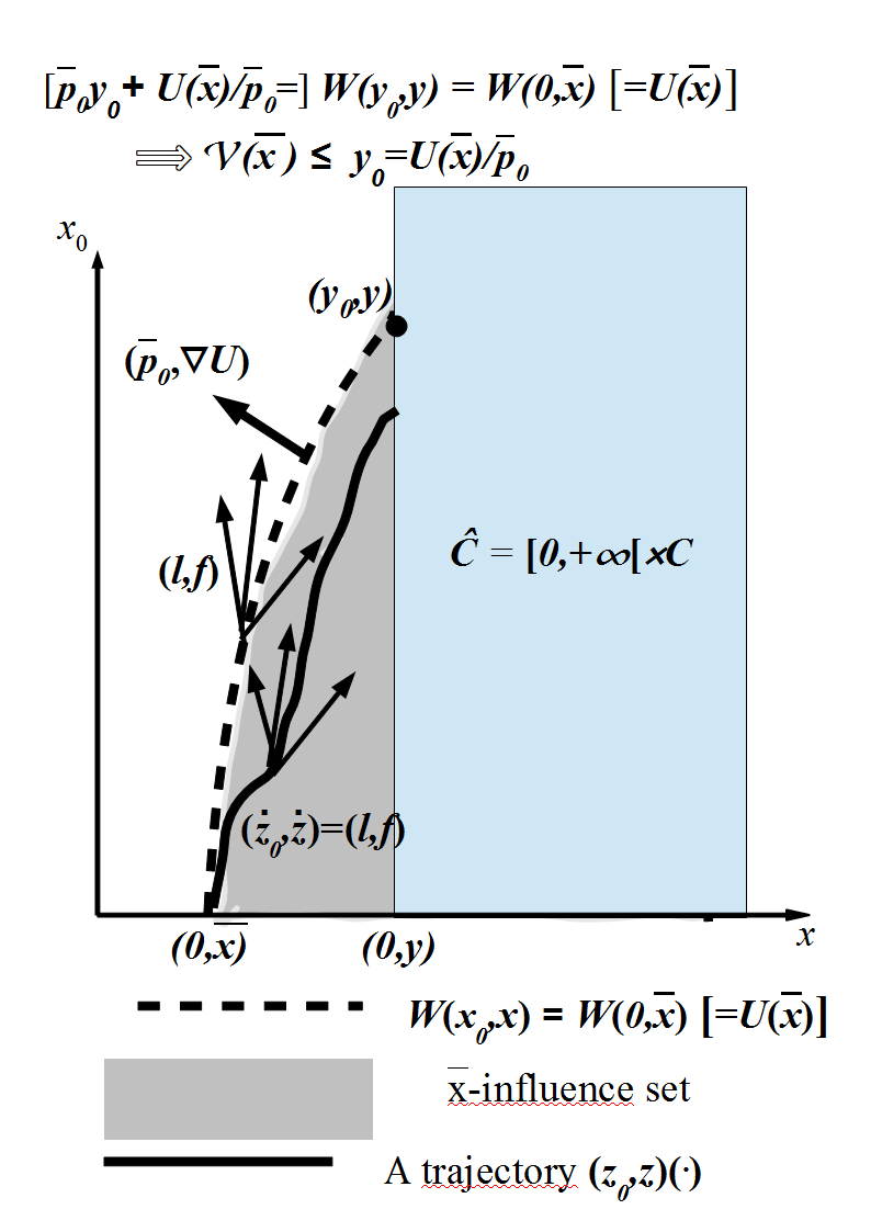
Figure 1: The level sets of $W$ intersect the extended target ${\hat{\bf C}}$

2.3 Some examples

Example 2.1

A prototype of (MRF) is a map of the form $U(x)=\Phi\circ{\bf d}(x)$, where $\Phi:[0,+\infty[\to{{{\rm I\mkern-3.5muR}}}$ is a continuous map such that $\Phi(0)=0$ and its restriction to $]0,+\infty[$ is a strictly increasing $C^{1}$-diffeomorphism.

In particular, in the minimum time problem, where $l\equiv 1$, the inequality (6) includes the following weak Petrov condition (see e.g. [S1], [CS], and [BP]):

• there exist $\delta>0$ and a continuous, increasing map $\mu:[0,\delta]\to[0,+\infty[$ verifying $\mu(0)=0$, $\mu(\rho)>0$ for $\rho>0$, $\displaystyle\int_{0}^{\delta}\frac{d\rho}{\mu(\rho)}<+\infty$, and such that, $\forall x\in{\bf C}^{c}$ with ${\bf d}(x)<\delta$, one has

  $$\inf_{a\in A}\langle D^{*}{\bf d}(x),f(x,a)\rangle\leq-\mu({\bf d}(x)).$$ (15)

Indeed, if we set $\Phi(r)\doteq\int_{0}^{r}\frac{d\rho}{\mu(\rho)}$ for all $r\in[0,\delta]$ and choose an arbitrary $\bar{p}_{0}\in[0,1[$, we can write (15) as

$$H(x,{\bar{p}_{0}},D^{*}(\Phi\circ{\bf d})(x))=\inf_{a\in A}\left\{{\bar{p}_{0}}+\left\langle D^{*}(\Phi\circ{\bf d})(x),f(x,a)\right\rangle\right\}\leq-(1-{\bar{p}_{0}})<0.$$

In particular, whenever $\Phi$ is linear one recovers the classical Petrov condition.

Example 2.2

Let $r,s$ be arbitrary real numbers and let $\psi_{1}(x)$, $\psi_{2}(x)$ be continuous functions such that $\psi_{1}(x)\geq M_{1}$ and $0\leq\psi_{2}(x)\leq M_{2}$ for some $M_{1}$, $M_{2}>0$. Consider the target ${\bf C}\doteq\{0\}$, the control dynamics

$$\dot{z}=a\,\psi_{1}(z)|z|^{r}\qquad a\in\{-1,1\}$$

and the Lagrangian

$$l(z)\doteq\psi_{2}(z)|z|^{s}.$$

Notice that $l$ can be zero on an arbitrary subset of its domain.

Let $s,r$ verify

$$s-r>-1$$ (16)

and consider the map

$$U(x)\doteq\frac{M_{2}}{M_{1}(s-r+1)}\,|x|^{s-r+1}.$$

Observe that $U$ is proper, positive definite and semiconcave on ${{{\rm I\mkern-3.5muR}}}\setminus\{0\}$ —actually, $U\in C^{\infty}({{{\rm I\mkern-3.5muR}}}\setminus\{0\})$. Moreover, for any $p_{0}\geq 0$,

$$\begin{array}[]{c}H(x,p_{0},p)=\inf_{a\in\{-1,1\}}\Big{\{}p_{0}\psi_{2}(x)\,|x|^{s}+ap\,\psi_{1}(x)\,|x|^{r}\Big{\}}\leq\\ \\ p_{0}M_{2}\,|x|^{s}-M_{1}\,|p||x|^{r}.\end{array}$$

Since

$$D^{*}U(x)=\left\{\nabla U(x)\right\}=\left\{\text{sign}(x)\,\frac{M_{2}}{M_{1}\,}|x|^{s-r}\right\}\qquad\forall x\neq 0,$$

one obtains

$$H(x,{\bar{p}_{0}},D^{*}U(x))<0\qquad\forall x\neq 0,$$

as soon as ${\bar{p}_{0}}\in]0,1[$.

By applying Theorem 1.1 we get that the value function ${\mathcal{V}}$ —namely, the minimum cost to attain the target (possibly in infinite time) —, verifies

$${\mathcal{V}}(x)\leq\frac{M_{2}}{M_{1}\bar{p}_{0}(s-r+1)}\,|x|^{s-r+1}\qquad\forall x\in{{{\rm I\mkern-3.5muR}}}$$

for all $\bar{p}_{0}\in]0,1[$, which implies

$${\mathcal{V}}(x)\leq\frac{M_{2}}{M_{1}(s-r+1)}\,|x|^{s-r+1}\qquad\forall x\in{{{\rm I\mkern-3.5muR}}}.$$

Notice that (16) is crucial. Indeed, if $s-r\leq-1$, a nonsingular (MRF) may fail to exists. In fact, consider the trivial case when $\psi_{1}=\psi_{2}\equiv 1$. If $U$ were a nonsingular (MRF), for almost every $x\in]0,1]$ we should have

$$|\nabla U(x)|>\bar{p}_{0}\,x^{s-r}\geq\bar{p}_{0}\,x^{-1}$$

for some $\bar{p}_{0}>0$, which clearly prevents $U$ to be positive definite.

In Example 2.2 the dynamics may happen to be unbounded (precisely, when $r<0$). However, when the time $T_{z}$ to approach the target happens to be finite, the trajectory’s interval can be prolonged to the closed interval $[0,T_{z}]$, so that $z(T_{z})\in{\bf C}$. Let us remark that this is due to the one-dimensionality of the state space. In fact in the next example we see, among other things, that there is a connected component of the target that can be approached in finite time while it cannot be reached.

Example 2.3

Let us set

$${\bf C}\doteq{\bf C}_{1}\cup{\bf C}_{2}\subset{{{\rm I\mkern-3.5muR}}}^{2},$$

where

$${\bf C}_{1}\doteq\{x\in{{{\rm I\mkern-3.5muR}}}^{2},\,\,\,|x|\leq 1\},\qquad{\bf C}_{2}\doteq\{x\in{{{\rm I\mkern-3.5muR}}}^{2},\,\,\,|x|\geq 4\},$$

and let us consider the control dynamics

$$\dot{z}=\frac{M\cdot z}{(|z|-1)}-\alpha z$$

with the control $\alpha$ taking values in $\{-1,1\}$ and $M\doteq\begin{pmatrix}\,\,0&1\\ -1&0\end{pmatrix}$. Finally let us consider the Lagrangian

$$l(x)\doteq\left\{\begin{array}[]{ll}(|z|-1)^{2}k(z)&\hbox{if}\,\,1\leq|z|\leq 2\\ (3-|z|)^{2}k(z)&\hbox{if}\,\,2<|z|\leq 3\\ 0&\hbox{if}\,\,3<|x|\leq 4\end{array}\right.,$$

where $k:{\bf C}^{c}\to{{{\rm I\mkern-3.5muR}}}$ is any continuous function verifying $0\leq k(z)\leq 1\,\,\,\,\forall z\in{\bf C}^{c}$. Let us begin with showing that the target’s component ${\bf C}_{1}$ can be indefinitely approached in finite time but it cannot be reached. Indeed, in polar coordinates $z=\rho e^{i\theta}$ the control equation becomes

$$\left\{\begin{array}[]{l}\dot{\rho}=-\alpha\rho\\ \\ \dot{\theta}=-(\rho-1)^{-1}\end{array}\right.$$

Let $\bar{\rho}\in]1,4[$, $\bar{\theta}\in[0,2\pi[$. Choose $\bar{z}=\bar{\rho}\,e^{i\bar{\theta}}\in{\bf C}^{c}$, $\alpha\equiv 1$, and consider the solution of the first equation: $\rho:[0,\ln\bar{\rho}[\to{{{\rm I\mkern-3.5muR}}}$, $\rho(t)\doteq\bar{\rho}\,e^{-t}$. The time this trajectory takes to approach ${\bf C}$ is equal to $\ln\bar{\rho}$. Furthermore,

$$\lim_{t\to\ln\bar{\rho}}(\rho(t),\theta(t))=(1,+\infty).$$

It follows that

$$\lim_{t\to\ln\bar{\rho}}{\bf d}(z(t))=0$$

but $z(t)$ has no limit as $t\to\ln\bar{\rho}$ . Namely, the trajectory spirals faster and faster around ${\bf C}_{1}$ while approaching it.

On the other hand it is trivial to see that the target’s component ${\bf C}_{2}$ can be reached in finite time by implementing the constant control $\alpha\equiv-1$. Lastly, setting for every $\epsilon\geq 0$,

$$U_{\epsilon}(z)\doteq\left\{\begin{array}[]{ll}2\epsilon+\frac{(|z|-1)^{3}}{3}&\hbox{if}\,\,1\leq|z|\leq 2\\ \\ \displaystyle\epsilon(4-|z|)+\frac{(3-|z|)^{3}}{3}&\hbox{if}\,\,2<|z|\leq 3\\ \\ \displaystyle\epsilon(4-|z|)&\hbox{if}\,\,3<|z|\leq 4\end{array}\right.,$$

one can easily check that as soon as $\epsilon>0$ $U_{\epsilon}$ is a Minimum Restraint Function with $\bar{p}_{0}=1$. Therefore, if ${{\mathcal{V}}}(x)$ denotes the value function of the problem, by Theorem 1.1 we get ${{\mathcal{V}}}(z)\leq U_{\epsilon}(z)$ for every $\epsilon>0$, so that

$${{\mathcal{V}}}(z)\leq U_{0}(z).$$ (17)

Notice that, in agreement with the definition of (MRF), the functions $U_{\epsilon}$ are not smooth at their maximum points. Moreover, the inequality (17) is optimal in the ring $R\doteq\{z\,\,|\,\,3\leq|z|\leq 4\}$, in that $U_{0}=0$, and hence ${{\mathcal{V}}}=0$, on $R$.

3 Proof of the main result

3.1 Preliminary results

The proof of Theorem 1.1 relies on Propositions 3.1 and 3.2 below. In order to retain clarity in the main proof’s argument, we postpone the proofs of these technical results to Section 4.

Proposition 3.1

Let $U$ be a (MRF) and let ${\bar{p}_{0}}\geq 0$ make (6) hold true, i.e.

$$H(x,{{\bar{p}_{0}}},D^{*}U(x))<0\qquad\forall x\in{{\bf C}}^{c}.$$

Then for every $\sigma>0$ the map $U$ verifies also the differential inequality

$$H(x,{{\bar{p}_{0}}},D^{*}U(x))\leq-m(U(x))\qquad\forall x\in U^{-1}(]0,\sigma[),$$ (18)

where $m:[0,+\infty[\to{{{\rm I\mkern-3.5muR}}}$ is a suitable continuous, strictly increasing function verifying $m(r)>0$   $\forall r>0$.

Remark 3.1

If we replace condition (6), namely

$$\exists{\bar{p}_{0}}:\ \ H(x,{{\bar{p}_{0}}},p)<0\qquad\forall x\in{\bf C}^{c},\ \ \forall p\in D^{*}U(x),$$

with the stronger assumption

$$\exists{\bar{p}_{0}}:\ \ \forall M>0,\quad\sup_{\,{\bf d}(x)\geq M;\ p\in D^{*}U(x)}H(x,{\bar{p}_{0}},p)<0,$$

then by slight changes in the proof of Proposition 3.1 below, one can prove that there exists a continuous, strictly increasing function $m:[0,+\infty[\to{{{\rm I\mkern-3.5muR}}}$, independent of $\sigma$, verifying $m(r)>0$   $\forall r>0$, such that (18) holds for all $x\in{\bf C}^{c}$.

Proposition 3.2

Let $U$ be a (MRF) and let $\sigma>0$. Let $m$ be defined as in Proposition 3.1. Fix $\varepsilon>0$ and $\bar{\mu}$, $\hat{\mu}$ such that $0<\hat{\mu}<\bar{\mu}<\sigma$. Then there is some $\delta>0$ such that, for every $\delta^{\prime}\in]0,\delta[$ and for each $x\in{\bf C}^{c}$ verifying $U(x)=\bar{\mu}$, for a suitable $\hat{t}>0$ one can construct a trajectory-control pair

$$(z,\alpha):[0,\hat{t}]\to U^{-1}([\hat{\mu},\bar{\mu}])\times A,\qquad z(0)=x,$$

and a finite partition $\pi=\{t^{0},\dots,t^{\bar{n}}\}$ of $[0,\hat{t}]$ such that diam$(\pi)\leq\delta^{\prime}$ and with the following properties:

• $U(z(\hat{t}))=\hat{\mu}<U(z(t))\leq U(z(0))=U(x)=\bar{\mu}$   $\forall t\in[0,\hat{t}[$;

• for every $j\in\{1,\dots,\bar{n}\}$ and $\forall t\in[t^{j-1},t^{j}[$,

  $$U(z(t^{j}))<U(z(t))\leq U(z(t^{j-1}));$$ (19)

• for every $j\in\{1,\dots,\bar{n}\}$ and $\forall t\in[t^{j-1},t^{j}]$,

  $$\begin{array}[]{l}U(z(t))-U(z(t^{j-1}))+\frac{\bar{p}_{0}}{\varepsilon+1}\int_{t^{j-1}}^{t}l(z(t),\alpha(t))\,dt\leq\\ \\ \qquad\qquad\qquad\qquad\qquad\qquad-\frac{1}{\varepsilon+1}\int_{t^{j-1}}^{t}m(U(z(t)))\,dt.\end{array}$$ (20)

3.2 Proof of Theorem 1.1.

In the sequel, given a constant $\mu>0$, for any continuous path $y:[\tau,+\infty[\to{{{\rm I\mkern-3.5muR}}}^{n}$ with $U(y(\tau))>\mu$, we define the time to reach the enlarged target $U^{-1}([0,\mu])$ as

$${\cal T}_{y}^{\mu}\doteq\inf\{r\geq\tau:\ U(y(r))\leq\mu\}$$ (21)

(${\cal T}_{y}^{\mu}=+\infty$ if $U(y(r))>\mu$ for all $r\geq\tau$).

Let $\sigma>0$ be a positive constant and let $m$ be defined as in Proposition 3.1. Fix $\varepsilon>0$ and let $(\nu_{k})\subset]0,1]$ be a sequence such that $1=\nu_{0}>\nu_{1}>\nu_{2}>\dots$ and $\lim_{k\to\infty}\nu_{k}=0$. Assume that $x\in U^{-1}(]0,\sigma[)$ and set

$$\mu_{k}\doteq\nu_{k}U(x)\quad\forall k\geq 0.$$

We are going to exploit Proposition 3.2 in order to build the trajectory-control pair

$$(z,\alpha):[0,\bar{t}[\to{\bf C}^{c}\times A$$

by concatenation,

$$(z(t),\alpha(t))=(z_{k}(t),\alpha_{k}(t))\quad\forall t\in[t_{k-1},t_{k}[,\quad\forall k\geq 1.$$

Step $k=1$. Let us begin by constructing $(z_{1},\alpha_{1})$. Setting $\bar{\mu}=\mu_{0}$, $\hat{\mu}=\mu_{1}$, let $(z_{1},\alpha_{1}):[0,\hat{t}]\to U^{-1}([\mu_{1},\mu_{0}])\times A$ be a trajectory built according to Proposition 3.2 such that $z_{1}(0)=x$. We set $t_{0}\doteq 0$ and $t_{1}\doteq\hat{t}$ and we observe that $t_{1}=T_{z_{1}}^{\mu_{1}}$, in view of (a) in Proposition 3.2.

Step $k>1$. Let us proceed by defining $(z_{k},\alpha_{k})$ for $k>1$. Setting $\bar{\mu}=\mu_{k-1}$, $\hat{\mu}=\mu_{k}$, let $(\hat{z}_{k},\hat{\alpha}_{k}):[0,\hat{t}]\to U^{-1}([\mu_{k},\mu_{k-1}])\times A$ be a trajectory built according to Proposition 3.2 such that $\hat{z}_{k}(0)=z_{k-1}(t_{k-1})$. We set $t_{k}\doteq t_{k-1}+\hat{t}$ and $(z_{k},\alpha_{k})(t)=(\hat{z}_{k},\hat{\alpha}_{k})(t-t_{k-1})$ $\forall t\in[t_{k-1},t_{k}]$. We observe that $t_{k}=T_{z_{k}}^{\mu_{k}}$, still in view of (a) in Proposition 3.2.

The concatenation procedure is concluded as soon as we set $\bar{t}\doteq\lim_{k\to\infty}t_{k}$. Notice that it may well happen that $\bar{t}=+\infty$. We claim that

$$\lim_{t\to\bar{t}^{-}}{\bf d}(z(t))=0.$$ (22)

For every $k\geq 1$, let us apply Proposition 3.2, which yields the existence of a finite partition $\pi_{k}=\{\hat{t}^{0}_{k},\dots,\hat{t}^{\bar{n}_{k}}_{k}\}$ of $[0,t_{k}-t_{k-1}]$ such that, setting,

$$t_{k}^{j}\doteq t_{k-1}+\hat{t}^{j}_{k}\qquad\forall j\in\{0,\dots,\bar{n}_{k}\},$$

one has $z(0)\,(=z_{1}(0))=x$, and, for every $k\geq 1$:

• $z_{k+1}(t_{k})=z_{k}(t_{k})$,   $U(z_{k}(t_{k-1}))=\mu_{k-1}$;

• for all $j\in\{1,\dots,\bar{n}_{k}\}$,
  $U(z_{k}(t_{k}^{j}))<U(z_{k}(t))\leq U(z_{k}(t_{k}^{j-1}))\leq U(x)$   $\forall t\in[t_{k}^{j-1},t_{k}^{j}[$;

• for all $j\in\{1,\dots,\bar{n}_{k}\}$,
  $U(z_{k}(t))-U(z_{k}(t_{k}^{j-1}))+\frac{\bar{p}_{0}}{\varepsilon+1}\int^{t}_{t_{k}^{j-1}}l(z_{k}(t),\alpha_{k}(t))\,dt\leq$
  mmmmmmmmmmmmmm $-\frac{1}{\varepsilon+1}\int^{t}_{t_{k}^{j-1}}m(U(z_{k}(t)))\,dt$   $\forall t\in[t_{k}^{j-1},t_{k}^{j}]$.

Indeed, in view of point (b)_k above, (22) is equivalent to

$$\lim_{k\to\infty}{\bf d}(z_{k}(t_{k}))=0.$$ (23)

On the other hand, since $U$ is proper and positive definite, (23) is a straightforward consequence of

$$\lim_{k\to\infty}U(z_{k}(t_{k}))=\lim_{k\to\infty}\nu_{k}\,U(x)=0$$

Therefore (22) is verified.

Notice that (b)_k implies also that

$$U(z(t))\leq U(x)<\sigma\quad\forall t\in[0,\bar{t}[.$$ (24)

In order to conclude the proof that the system is (GAC) to ${\bf C}$ (part (i) of the theorem), we have to establish the existence of a ${\cal KL}$ function $\beta$ as in Definition 1.5.

Let $k\geq 1$. From condition (c)_k and in view of the definition of $(z_{k},\alpha_{k})$, we have $\forall t\in[t_{k-1},t_{k}^{j}]$,

$$\begin{array}[]{l}U(z_{k}(t))-U(z_{k}(t_{k-1}))=[U(z_{k}(t))-U(z_{k}(t_{k}^{j-1}))]+[U(z_{k}(t_{k}^{j-1}))-U(z_{k}(t_{k}^{j-2}))]\\ \\ \qquad+\dots+[U(z_{k}(t_{k}^{1}))-U(z_{k}(t_{k}^{0}))]\leq\\ \\ \qquad\qquad\qquad\qquad-\frac{\bar{p}_{0}}{\varepsilon+1}\int^{t}_{t_{k-1}}l(z_{k}(\tau),\alpha_{k}(\tau))\,d\tau-\frac{1}{\varepsilon+1}\int^{t}_{t_{k-1}}m(U(z_{k}(\tau)))\,d\tau,\end{array}$$

which implies that $\forall t\in[0,t_{k}^{j}]$,

$$U(z(t))-U(x)\leq-\frac{\bar{p}_{0}}{\varepsilon+1}\int^{t}_{0}l(z(\tau),\alpha(\tau))\,d\tau-\frac{1}{\varepsilon+1}\int^{t}_{0}m(U(z(\tau)))\,d\tau.$$ (25)

Being $l\geq 0$, in particular we have

$$U(z(t))-U(x)\leq-\frac{\int^{t}_{0}m(U(z(\tau))\,d\tau}{\varepsilon+1}.$$

Since $\min\{m(U(z(\tau)):\ \tau\in[0,t_{k}^{j}]\}=m(U(z(t_{k}^{j}))$, we get

$$U(z(t))+\frac{m(U(z(t_{k}^{j}))\,t}{\varepsilon+1}\leq U(x)\qquad\forall t\in[0,t_{k}^{j}].$$ (26)

Observe that the function $\tilde{m}:[0,+\infty[\to[0,+\infty[$ defined by $\tilde{m}(r)\doteq\min\{r,m(r)\}$ for all $r\in[0,+\infty[$ is continuous, strictly increasing, and $\tilde{m}(r)>0$   $\forall r>0$, $\tilde{m}(0)=0$. Then, for any $k\geq 1$ and for any $j\in\{1,\dots,{\bar{n}_{k}}\}$,

$$\tilde{m}(U(z(t_{k}^{j}))\left[1+\frac{t_{k}^{j}}{\varepsilon+1}\right]\leq U(x),$$

so that

$$U(z(t_{k}^{j}))\leq\tilde{m}^{-1}\left(\frac{\varepsilon+1}{\varepsilon+1+t_{k}^{j}}\,U(x)\right).$$

Let $t\in[0,\bar{t}[$. Then $t\in[t_{k}^{j-1},t_{k}^{j}[$ for some $k\geq 1$ and some $j\in\{0,\dots,{\bar{n}_{k}}\}$. Moreover, by possibly reducing $diam(\pi_{k})$ (see Proposition 3.2), we can obtain $t_{k}^{j}-t_{k}^{j-1}\leq\bar{\delta}$, with $\bar{\delta}$ so small that

$$\omega_{\tilde{m}}(LM_{f}\bar{\delta})\leq\tilde{m}(\mu_{k})\frac{\varepsilon}{1+2\varepsilon}.$$ (27)

Here $\omega_{\tilde{m}}$ denotes the modulus of continuity of $\tilde{m}$, when restricted to $[\mu_{k+1},\sigma]$, $L$ is the Lipschitz constant of $U$ on $U^{-1}([\mu_{k+1},\sigma])$ and $M_{f}$ is the supremum of $|f|$ on $U^{-1}([\mu_{k+1},\sigma])\times A$. Hence

$$\tilde{m}(U(z(t_{k}^{j}))\geq\tilde{m}(U(z(t))\frac{1+\varepsilon}{1+2\varepsilon},$$ (28)

which, together with (26), implies that

$$U(z(t))\leq\tilde{m}^{-1}\left(\frac{2\varepsilon+1}{2\varepsilon+1+t}\,U(x)\right).$$

Let us set

$$\sigma_{-}(r)\doteq\min\{{\bf d}(z):\ U(z)\geq r\},\quad\sigma^{+}(r)\doteq\max\{{\bf d}(z):\ U(z)\leq r\}.$$ (29)

Notice that $\sigma_{-}$, $\sigma^{+}:[0,+\infty[\to{{{\rm I\mkern-3.5muR}}}$ are continuous, strictly increasing, unbounded functions such that $\sigma_{-}(0)=\sigma^{+}(0)=0$ and

$$\forall z\in{U^{-1}([0,\sigma[)}:\quad\sigma_{-}(U(z))\leq{\bf d}(z);\quad\sigma^{+}(U(z))\geq{\bf d}(z).$$

Moreover, it is not restrictive to replace $\sigma_{-}(r)$ with $\min\{\sigma_{-}(r),r\}$. Let us define $\beta:[0,+\infty[\times[0,+\infty[\to[0,+\infty[$ by setting

$$\beta(r,t)\doteq\sigma^{+}\circ\tilde{m}^{-1}\left(\sigma_{-}^{-1}(r)\,\frac{2\varepsilon+1}{2\varepsilon+1+t}\right).$$ (30)

Therefore by straightforward calculations it follows that

$${\bf d}(z(t))\leq\beta({\bf d}(x),t)\qquad\forall t\in[0,T_{z}[.$$

It implies that, starting from any initial point $x\in U^{-1}(]0,\sigma[)$,

$${\bf d}(z(t))\leq\beta({\bf d}(x),t)\qquad\forall t\in[0,+\infty[.$$

Let us recall that, in case $T_{z}<+\infty$, we mean that $z(t)\doteq\bar{z}$   $\forall t\geq T_{z}$, for some $\bar{z}\in\partial{\bf C}$ (see the footnote to Definition 1.5). By the arbitrariness of $\sigma>0$, it is easy to extend the construction of $\beta$ from $U^{-1}([0,\sigma])\times[0,+\infty[$ to the whole set ${\bf C}^{c}\times[0,+\infty[$.

On the one hand, this concludes the proof of part (i) of the theorem. On the other hand, the proof of (ii) is straightforward, since in view of (25) we have

$$\int_{0}^{\bar{t}}l(z(t),\alpha(t))\,dt=\lim_{k\to+\infty}\int_{0}^{t_{k}}l(z(t),\alpha(t))\,dt\leq\frac{(\varepsilon+1)}{\bar{p}_{0}}\,U(x),$$

which implies (7).

4 Proofs of some technical results

4.1 Proof of Proposition 3.1.

In order to prove (18) let us observe that by the definition of $U$, for any $\sigma>0$, $U^{-1}([0,\sigma])$ is compact. Moreover, for every $\delta\in]0,\sigma]$ the graph of the restriction of the set-valued map $x\to D^{*}U(x)$ to $U^{-1}({[\delta,\sigma]})$, namely the set

$$\Gamma_{\delta}\doteq\left\{(x,p):\ \ x\in U^{-1}({[\delta,\sigma]}),\ p\in D^{*}U(x)\right\},$$

is compact. Indeed the set-valued map, $x\to D^{*}U(x)$ is upper semicontinuous with compact values (see e.g. [AC]). Therefore the continuous function $(x,p)\mapsto H(x,{{\bar{p}_{0}}},p)$ has a maximum on $\Gamma_{\delta}$. For every $\delta\in]0,\sigma]$, let us set

$$\hat{m}(\delta)\doteq-\max_{(x,p)\in\Gamma_{\delta}}\,H(x,{{\bar{p}_{0}}},p)\,\,(>0).$$

Notice that the function $\hat{m}$ is positive and increasing. Furthermore, it is lower semicontinuous. Finally, for every $x\in U^{-1}({]0,\sigma[})$ one has

$$H(x,{{\bar{p}_{0}}},p)\leq-\hat{m}(U(x))\qquad\forall p\in D^{*}U(x).$$

The thesis is now proved by choosing, for any $\sigma>0$, a continuous, strictly increasing, function $m:[0,+\infty[\to[0,+\infty[$ such that $0<m(r)\leq\hat{m}(r)$ for every $r\in]0,\sigma]$ and $m(0)\geq 0$.

4.2 Proof of Proposition 3.2

Let $(\zeta,\alpha)$ be a trajectory-control pair verifying conditions (a)–(f) of Lemma 4.1 below. Set $t^{0}\doteq 0$ and, for every $j\in\{1,\dots,\bar{n}\}$, define

$$\tau^{j}(s)\doteq t^{j-1}+\int_{s^{j-1}}^{s}\frac{1}{\bar{p}_{0}l(\zeta^{j}(\sigma),a^{j})+m(U(\zeta^{j}(\sigma)))}\,d\sigma\quad\forall s\in[s^{j-1},s^{j}],\quad t^{j}\doteq\tau^{j}(s^{j}).$$

Set $\hat{t}\doteq t^{\bar{n}}$. It is trivial to verify that:

• for every $j\in\{1,\dots,\bar{n}\}$, the path

  $$z^{j}:t\mapsto z^{j}(t)\doteq\zeta^{j}\circ(\tau^{j})^{-1}(t)\qquad t\in[t^{j-1},t^{j}].$$

  is a trajectory of the original system in (2) with initial condition $z^{j}(t^{j-1})=x^{j}$, corresponding to the constant control $a^{j}$;

• the trajectory-control pair $(z,\alpha):[0,\bar{t}]\to U^{-1}([\hat{\mu},\bar{\mu}])\times A$ given by

  $$(z(t),\alpha(t))\doteq(z^{j}(t),a^{j})\quad t\in[t^{j-1},t^{j}[\quad(j\in\{1,\dots,\bar{n}\}),$$

  satisfies conditions (a)–(c) of Proposition 3.2.

Lemma 4.1

Let $U$ be a (MRF), let $\sigma>0$, and fix a selection $p(x)\in D^{*}U(x)$. Let $m$ be defined as in Proposition 3.1 when $\sigma$ is replaced with $\sigma+2$, and let $x\mapsto a(x)\in A$ be a feedback lawverifying

$$\left\langle p(x)\,,\,\frac{f(x,a(x))}{\bar{p}_{0}\,l(x,a(x))+m(U(x))}\right\rangle\leq-1\qquad\forall x\in U^{-1}(]0,\sigma+2[).$$ (31)

Fix $\varepsilon>0$ and $\bar{\mu}$, $\hat{\mu}$ such that $0<\hat{\mu}<\bar{\mu}<\sigma$.

Then there exists $\delta>0$ such that, for every partition $\pi=(s^{j})$ of $[0,+\infty[$ with diam$(\pi)\leq\delta$, for each $x\in{\bf C}^{c}$ verifying $U(x)=\bar{\mu}$, there is a map $(\zeta,\alpha):[0,\bar{s}]\to U^{-1}([\hat{\mu},\bar{\mu}])\times A$ verifying

$$(\zeta(s),\alpha(s))\doteq(\zeta^{j}(s),a^{j})\quad\forall s\in[s^{j-1},s^{j}[\quad(j\geq 1),$$

and a sequence $(x^{1},x^{2},\dots)\in U^{-1}([0,\bar{\mu}])$, where:

• $\zeta^{1}(s^{0})=x\doteq x^{1}$; for every $j>1$, $\zeta^{j}(s^{j-1})=\zeta^{j-1}(s^{j-1})\doteq x^{j}$;

• for every $j\geq 1$, $\zeta^{j}:[s^{j-1},s^{j}]\to{{{\rm I\mkern-3.5muR}}}^{n}$ is a solution of the Cauchy problem

  $$\frac{d\zeta}{ds}=\frac{f(\zeta,a^{j})}{\bar{p}_{0}\,l(\zeta,a^{j})+m(U(\zeta))},\quad\zeta(s^{j-1})=x^{j},$$

  where

  $$a^{j}\doteq a(x^{j});$$ (32)

• ${\cal T}^{\hat{\mu}}_{\zeta}<+\infty$ and $\bar{s}\doteq{\cal T}^{\hat{\mu}}_{\zeta}$;

• for every $j\geq 1$ such that $s^{j-1}<\bar{s}$, one has

  $$U(\zeta^{j}(s))-U(x^{j})\leq-\frac{s-s^{j-1}}{\varepsilon+1}\qquad\forall s\in[s^{j-1},s^{j}];$$ (33)

• $U(\zeta(\bar{s}))=\hat{\mu}<U(\zeta(s))\leq U(\zeta(0))=U(x)=\bar{\mu}$   $\forall s\in[0,\bar{s}[$, and

  $$\bar{s}\leq(\varepsilon+1)\,U(x).$$ (34)

Moreover, it is possible to choose the partition $\pi$ in such a way that

• $\bar{s}=s^{\bar{n}}$ for some integer $\bar{n}\geq 1$, and, for every $j\in\{1,\dots,\bar{n}\}$,

  $$U(\zeta(s^{j}))<U(\zeta(s))\leq U(\zeta(s^{j-1})\quad\forall s\in[s^{j-1},s^{j}[.$$ (35)

Proof. Fix $\varepsilon>0$ and set

$$g(x,a)\doteq\bar{p}_{0}\,l(x,a)+m(U(x))$$ (36)

for all $(x,a)\in U^{-1}({[{\hat{\mu}/2},{\sigma+1}]})\times A$. For any continuous function $\phi:{{{{\rm I\mkern-3.5muR}}}^{n}}\times A\to{{{\rm I\mkern-3.5muR}}}^{q}$, we use $M_{\phi}$, and $\omega_{\phi}(\cdot)$ to denote the sup-norm and the modulus of continuity of $\phi$ in $U^{-1}({[{\hat{\mu}/2},{\sigma+1}]})\times A$, respectively. In case $\phi$ is scalar valued, let us use $m_{\phi}$ to denote the minimum of $\phi$ on $U^{-1}({[{\hat{\mu}/2},{\sigma+1}]})\times A$. Finally, since $U$ is locally semiconcave, there exist $R$, $\rho>0$, $L>0$ such that for all $\hat{x}\in B_{n}(x,R)\cap U^{-1}({[{\hat{\mu}/2},{\sigma+1}]})$ one has

$$U(\hat{x})-U(x)\leq\langle p,\hat{x}-x\rangle+\rho\,|\hat{x}-x|^{2}\qquad\forall p\in D^{*}U(x),$$ (37)

$$|p|\leq L\qquad\forall p\in D^{*}U(x).$$ (38)

Let $\psi:{{{\rm I\mkern-3.5muR}}}^{n}\to[0,1]$ be a $C^{\infty}$ (cut-off) map such that

$$\psi=1\quad\hbox{on}\quad U^{-1}([{\hat{\mu}/2},\sigma]),\qquad\psi=0\quad\hbox{on}\,\,\,I\!\!R^{n}\backslash U^{-1}([{\hat{\mu}/4},{\sigma+1}])$$ (39)

Let us set

$$\delta\doteq\min\{\delta_{1},\delta_{2},\hat{\mu}/2\},$$

where

$$\delta_{1}\doteq\frac{R\,m_{g}}{M_{f}},$$ (40)

and $\delta_{2}>0$ is any positive real number such that

$$L\,\omega_{(\psi\,\frac{f}{g})}\left(\frac{M_{f}}{m_{g}}\,r\right)+\rho\,\frac{M_{f}^{2}}{m_{g}^{2}}\,r\leq\frac{\varepsilon}{\varepsilon+1}\qquad\forall r\in]0,\delta_{2}].$$ (41)

Let $\pi=(s^{j})$ be an arbitrary partition of $[0,+\infty[$ such that diam$(\pi)\leq\delta$. For each $x\in{\bf C}^{c}$ verifying $U(x)=\bar{\mu}$, define recursively a sequence of trajectory-control pairs $(\zeta^{j},\alpha^{j}):[s^{j-1},s^{j}]\to{{{\rm I\mkern-3.5muR}}}^{n}\times A$, $j\geq 1$, as follows:

$$\zeta^{1}(s^{0})\doteq x^{1}\doteq x,\ \ a^{1}\doteq a(x^{1});$$

for every $j>1$,

$$\zeta^{j}(s^{j-1})\doteq\zeta^{j-1}(s^{j-1})\doteq x^{j},\quad a^{j}\doteq a(x^{j});$$

for every $j\geq 1$, $\zeta^{j}:[s^{j-1},s^{j}]\to{{{\rm I\mkern-3.5muR}}}^{n}$ is a solution of the Cauchy problem

$$\frac{d\zeta}{ds}=\psi(\zeta)\,\frac{f(\zeta,a^{j})}{g(\zeta,a^{j})},\quad\zeta(s^{j-1})=x^{j}.$$

Notice that, by the continuity of the vector field and because of the cut-off factor $\psi$, any trajectory $\zeta^{j}(\cdot)$ exists globally and cannot exit the compact subset $U^{-1}({[{\hat{\mu}/4},{\sigma+1}]})$. Let us set

$$(\zeta(s),\alpha(s))\doteq(\zeta^{j}(s),a^{j})\ \ \forall s\in[s^{j-1},s^{j}[,\quad\text{for every $j\geq 1$.}$$

Since, for every $j\geq 1$, one has that $s^{j}-s^{j-1}\leq\delta\leq\delta_{1}$, by (40) it follows that $|\zeta^{j}(s)-x^{j}|\leq R$   $\forall s\in[s^{j-1},s^{j}]$. Hence, recalling that $|\psi|\leq 1$ and $\psi(x^{j})=1$ as soon as $x^{j}\in U^{-1}([\hat{\mu}/2,\sigma+1])$, (37) and (31) imply that, for every $j\geq 1$ such that $s^{j-1}<{\cal T}^{\hat{\mu}}_{\zeta}$ (see Definition 21), one has, $\forall s\in[s^{j-1},s^{j}]$,

$$\begin{array}[]{l}U(\zeta^{j}(s))-U(x^{j})\leq\langle p(x^{j}),\zeta^{j}(s)-x^{j}\rangle+\rho|\zeta^{j}(s)-x^{j}|^{2}=\\ \\ \left\langle p(x^{j}),\int_{s^{j-1}}^{s}{\psi(\zeta^{j}(\tau))\,\frac{f(\zeta^{j}(\tau),a^{j})}{g(\zeta^{j}(\tau),a^{j})}\,d\tau}\right\rangle+\rho\left|\int_{s^{j-1}}^{s}\psi(\zeta^{j}(\tau))\,\frac{f(\zeta^{j}(\tau),a^{j})}{g(\zeta^{j}(\tau),a^{j})}\,d\tau\right|^{2}\leq\\ \\ \left\langle p(x^{j}),\int_{s^{j-1}}^{s}\left[\psi(\zeta^{j}(\tau))\,\frac{f(\zeta^{j}(\tau),a^{j})}{g(\zeta^{j}(\tau),a^{j})}-\frac{f(x^{j},a^{j})}{g(x^{j},a^{j})}\right]\,d\tau\right\rangle+\left\langle p(x^{j}),\frac{f(x^{j},a^{j})}{g(x^{j},a^{j})}\right\rangle\,(s-s^{j-1})+\\ \\ \rho\left(\int_{s^{j-1}}^{s}\left|\psi(\zeta^{j}(\tau))\frac{f(\zeta^{j}(\tau),a^{j})}{g(\zeta^{j}(\tau),a^{j})}\right|\,d\tau\right)^{2}\leq\\ \\ L\,\omega_{(\psi\,\frac{f}{g})}\left(\frac{M_{f}}{m_{g}}\,(s^{j}-s^{j-1})\right)\,(s-s^{j-1})+\rho\,\frac{M_{f}^{2}}{m_{g}^{2}}\,(s-s^{j-1})^{2}-(s-s^{j-1})\leq\\ \\ \left[L\,\omega_{(\psi\,\frac{f}{g})}\left(\frac{M_{f}}{m_{g}}\,(s^{j}-s^{j-1})\right)+\rho\,\frac{M_{f}^{2}}{m_{g}^{2}}\,(s^{j}-s^{j-1})-1\right](s-s^{j-1}).\end{array}$$

Since $\forall s\in[s^{j-1},s^{j}]$, $s-s^{j-1}\leq\delta\leq\delta_{2}$, by (41) it follows that

$$U(\zeta^{j}(s))-U(x^{j})\leq-\frac{s-s^{j-1}}{\varepsilon+1},$$ (42)

which implies

$$U(\zeta(s))-U(x)=[U(\zeta^{j}(s))-U(x^{j})]+\dots+[U(\zeta^{1}(s^{1})-U(x)]\leq-\frac{s}{\varepsilon+1}.$$ (43)

In particular, (43) yields that $U(\zeta(s))\leq\bar{\mu}$ for all $s\in[0,s^{j}]$.

Notice that ${\cal T}^{\hat{\mu}}_{\zeta}<+\infty$. Indeed, if by contradiction ${\cal T}^{\hat{\mu}}_{\zeta}=+\infty$, (43) held true for all $s\in[0,s^{j}]$ with $j$ arbitrarily large, i.e. (since $(s^{j})$ is a partition of $[0,+\infty[$), for all $s\geq 0$. Therefore one would have $\lim_{s\to+\infty}U(\zeta(s))=0$, which is not allowed, since

$$U(\zeta(s))>\hat{\mu}\qquad\forall s\in[0,{\cal T}^{\hat{\mu}}_{\zeta}[.$$ (44)

Let us set

$$\bar{s}\doteq\bar{\cal T}^{\hat{\mu}}_{\zeta}(<+\infty),$$

and

$$\quad\bar{n}\doteq\sup\{j\geq 1:s^{j-1}<\bar{s}\}.$$

Let us observe that $\bar{n}<+\infty$.

Finally, notice that, because of (44), $\psi(\zeta(s))=1$ for every $s\in[0,s^{\bar{n}}]$. Hence, for any $j\in\{1,\dots,\bar{n}\}$, $\zeta^{j}(\cdot)$ is a solution of

$$\frac{d\zeta}{ds}=\frac{f(\zeta,a^{j})}{g(\zeta,a^{j})}\ \ \forall s\in[s^{j-1},s^{j}],\quad\zeta(s^{j-1})=x^{j}.$$

It follows that conditions (a)–(e) are satisfied. Notice however that in general (f) does not hold. Indeed it may happen that $s^{\bar{n}}>\bar{s}$. In addition, the first inequality of (35), namely $U(\zeta(s^{j}))<U(\zeta(s))$, may fail to be verified for some $s\in]s^{j-1},s^{j}[$.

In order to prove (f), it is sufficient to slightly refine the previous construction:

• In case (35) does not hold in $[0,\delta]$, redefine $s^{1}$ by setting $s^{1}\doteq\inf\{s\in]\hat{0},\delta]:\ U(\zeta^{1}(s))\leq U(\zeta^{1}(\delta))\}$.

• For every $j>1$, choose $a^{j}$ and $\zeta^{j}:[s^{j-1},s^{j-1}+\delta]\to{{{\rm I\mkern-3.5muR}}}^{n}$ with the same procedure we have followed in the previous construction. In case (35) does not hold in $[s^{j-1},s^{j-1}+\delta]$, set $s^{j}\doteq\inf\{s\in]s^{j-1},s^{j-1}+\delta]:\ U(\zeta^{j}(s))\leq U(\zeta^{j}(s^{j-1}+\delta))\}$.

The trajectory $\zeta$ defined by setting $\zeta(s)\doteq\zeta^{j}(s)$   $\forall s\in[s^{j-1},s^{j}[$, $j\geq 1$, verifies (35). It remains to prove that $(\bar{s}=)\,{\cal T}^{\hat{\mu}}_{\zeta}=s^{\bar{n}}$ for some integer $\bar{n}$. Begin with observing that $U(x^{j+1})=U(\zeta^{j}(s^{j}))=U(\zeta^{j}(s^{j-1}+\delta))$. Hence, by (42) it follows that

$$U(x^{j+1})-U(x^{j})=U(\zeta^{j}(s^{j-1}+\delta))-U(\zeta^{j}(\ s^{j-1}))\leq-\frac{\delta}{\varepsilon+1},$$

so that

$$U(x^{j+1})\leq U(x)-\frac{j\delta}{\varepsilon+1}.$$

Since $j\in{{{\rm I\mkern-3.5muN}}}$, we get $s^{\bar{n}}={\cal T}^{\hat{\mu}}_{\zeta}$ for some integer $\bar{n}$ smaller than the first $n$ such that $n\delta>(\varepsilon+1)(\bar{\mu}-\hat{\mu})$.

5 A remark on supersolutions

The notion of (MRF) can be restated by replacing the strict inequality (6) with a supersolution condition.

Preliminarly, let us recall some basic facts from nonsmooth analysis. We remind that we are using $\partial_{{\bf C}}F$ and $D^{*}F$ to denote the Clarke’s generalized gradient and the set of limiting gradients, respectively (see Definition 1.4).

Definition 5.1

Let $\Omega\subset{{{\rm I\mkern-3.5muR}}}^{n}$ be an open set, and let $F:\Omega\to{{{\rm I\mkern-3.5muR}}}$ be a locally bounded function. For every $x\in\Omega$, the set

$$\quad D^{-}F(x)\doteq\left\{p\in{{{\rm I\mkern-3.5muR}}}^{n}:\ \ \liminf_{y\to x}\frac{F(y)-F(x)-\langle p,(y-x)\rangle}{|y-x|}\geq 0\right\},$$

is called the subdifferential of $F$.

We recall that $D^{-}F(x)$ is a closed, convex (possibly empty) set. If $F$ is differentiable at $x$, then $D^{-}F(x)=\{\nabla F(x)\}$. Moreover, when $F$ is locally Lipschitz, $D^{-}F(x)\subset\partial_{{\bf C}}F(x)=co\,D^{*}F(x)$.

Proposition 5.1

Let $U:\overline{{\bf C}^{c}}\to{{{\rm I\mkern-3.5muR}}}$ be a (MRF) and let $\bar{p}_{0}\geq 0$ be the constant for which (6) holds true. Then the strict inequality (6) can be equivalently replaced by the following condition:

• for every $\sigma>0$, there exists a continuous, strictly increasing function $m=m_{\sigma}:[0,+\infty[\to{{{\rm I\mkern-3.5muR}}}$ verifying $m(r)>0$   $\forall r>0$, such that $U$ is a viscosity supersolution of equation $-H(x,{{\bar{p}_{0}}},Du)-m(u)=0$ in $U^{-1}(]0,\sigma[)$, namely, one has

  $$H(x,{{\bar{p}_{0}}},D^{-}U(x))\leq-m(U(x))\quad\forall x\in U^{-1}(]0,\sigma[).$$ (45)

Proof.  In view of Proposition 3.1, in order to show that (45) implies (6) it is enough to prove that, for any $\sigma>0$, (45) implies

$$H(x,{{\bar{p}_{0}}},D^{*}U(x))\leq-m(U(x))\quad\forall x\in U^{-1}(]0,\sigma[)$$ (46)

(for the same function $m$ as in (45)). For any $x\in U^{-1}(]0,\sigma[)$ and $p\in D^{*}U(x)$, there is a sequence $(x_{n})\subset U^{-1}(]0,\sigma[)\cap\,DIFF(U)$ such that $\lim_{n}(x_{n},\nabla U(x_{n}))=(x,p)$. Since

$$D^{-}U(x)=\{\nabla U(x)\}\quad\forall x\in DIFF(U),$$ (47)

by hypothesis (45) one has

$$H\left(x_{n},\,{{\bar{p}_{0}}},\,\nabla U(x_{n})\right)\leq-m(U(x_{n})),$$

for each natural number $n$. Passing to the limit an $n$ tends to infinity we get (46). The converse implication is a straightforward consequence of the following relations (see e.g. [CS]):

$$\begin{array}[]{l}D^{*}U(x)=D^{-}U(x)=\{\nabla U(x)\}\quad\forall x\in DIFF(U);\\ \\ D^{-}U(x)=\emptyset\quad\forall x\in{\bf C}^{c}\setminus DIFF(U).\end{array}$$ (48)

Acknowledgments. The authors thank Fabio Priuli and the anonymous referees for carefully reading the paper and making useful comments.

References

- [AB] F. Ancona & A. Bressan (1999) Patchy vector fields and asymptotic stabilization. ESAIM Control Optim. Calc. Var. 4, 445 471.
- [AC] J.P. Aubin & A. Cellina, (1984) Differential inclusions. Set-valued maps and viability theory. Grundlehren der Mathematischen Wissenschaften [Fundamental Principles of Mathematical Sciences], 264. Springer-Verlag, Berlin.
- [BCD] M. Bardi & I. Capuzzo Dolcetta, (1997) Optimal control and viscosity solutions of Hamilton-Jacobi-Bellman equations, Ed. Birkhäuser, Boston.
- [BP] A. Bressan & B. Piccoli, (2007) Introduction to the mathematical theory of control. AIMS Series on Applied Mathematics, 2. American Institute of Mathematical Sciences (AIMS), Springfield, MO.
- [CSic] F. Camilli, A. Siconolfi, (1999) Maximal subsolution for a class of degenerate Hamilton-Jacobi problems, Indiana Univ. Math. Journal, vol. 48, p. 1111–1131.
- [CS] P. Cannarsa & C. Sinestrari (2004). Semiconcave functions, Hamilton-Jacobi equations, and optimal control. Progress in Nonlinear Differential Equations and their Applications, 58. Birkhäuser Boston, Inc., Boston, MA.
- [CLSS] F. Clarke, Y. Ledyaev, E. Sontag, A. Subbotin, (1997) Asymptotic controllability implies feedback stabilization. IEEE Trans. Automat. Control 42 , no. 10, 1394–1407.
- [I] H. Ishii (1987) A simple direct proof of uniqueness for solutions of Hamilton-Jacobi equations of Eikonal type. Proc. Am. Math. Soc., vol. 100, 247-251
- [IR] H. Ishii, M. Ramaswamy (1995) Uniqueness results for a class of Hamilton-Jacobi equations with singular coefficients. Comm. Par. Diff. Eq., vol. 20, 2187-2213
- [Ma] M. Malisoff (2004).Bounded-from-below solutions of the Hamilton-Jacobi equation for optimal control problems with exit times: vanishing Lagrangians, eikonal equations, and shape-from-shading. NoDEA Nonlinear Differential Equations Appl., vol. 11, p. 95–122.
- [MaRS] M. Malisoff, L. Rifford, E. Sontag (2004). Global asymptotic controllability implies input-to-state stabilization. SIAM J. Control Optim. 42, no. 6, 2221–2238.
- [M] M. Motta, (2004) Viscosity solutions of HJB equations with unbounded data and characteristic points. Appl. Math. Optim. 49, no. 1, 1–26.
- [MS] M. Motta and C. Sartori, (2011) On some infinite horizon cheap control problems with unbounded data. 18th IFAC World Congress, Milan, Italy.
- [S1] E.D. Sontag (1998). Mathematical control theory. Deterministic finite-dimensional systems. Second edition. Texts in Applied Mathematics, 6. Springer-Verlag, New York.
- [S2] E. Sontag (1983) A Lyapunov-like characterization of asymptotic controllability. SIAM J. Control Optim. 21, no. 3, 462-471.
- [Sor1] P. Soravia (1993). Pursuit-evasion problems and viscosity solutions of Isaacs equations. SIAM J. of Control and Optimization, vol 1, n. 3, p. 604–623.
- [Sor2] P. Soravia (1999). Optimality principles and representation formulas for viscosity solutions of Hamilton-Jacobi equations I: Equations of unbounded and degenerate control problems without uniqueness. Adv. Differential Equations, p.275–296.