Stationary correlations for the 1D KPZ equation

Abstract

We study exact stationary properties of the one-dimensional Kardar-Parisi-Zhang (KPZ) equation by using the replica approach. The stationary state for the KPZ equation is realized by setting the initial condition the two-sided Brownian motion (BM) with respect to the space variable. Developing techniques for dealing with this initial condition in the replica analysis, we elucidate some exact nature of the height fluctuation for the KPZ equation. In particular, we obtain an explicit representation of the probability distribution of the height in terms of the Fredholm determinants. Furthermore from this expression, we also get the exact expression of the space-time two-point correlation function.

1 Introduction

Surface growth phenomena have attracted much attention in both science and technology, which involve fundamental understanding of the roughness of the surface and applications to the design of new materials. Being typical nonlinear and nonequilibrium phenomena, they have been one of the main topics in nonequilibrium statistical physics. In 1986, Kardar, Parisi and Zhang proposed a prototypical equation which describes surface growth with local interaction [1]. Its one-dimensional version reads

$$\frac{\partial h(x,t)}{\partial t}=\frac{\lambda}{2}\left(\frac{\partial h(x,t)}{\partial x}\right)^{2}+\nu\frac{\partial^{2}h(x,t)}{\partial x^{2}}+\sqrt{D}\eta(x,t).$$ (1.1)

Here $h(x,t)$ represents the height of the surface at position $x\in\mathbb{R}$ and time $t\geq 0$. The first term represents the effect of nonlinearity and the second one describes the smoothing effect of the surface. $\eta(x,t)$ represents randomness described by the Gaussian white noise with covariance,

$$\langle\eta(x,t)\eta(x^{\prime},t^{\prime})\rangle=\delta(x-x^{\prime})\delta(t-t^{\prime}).$$ (1.2)

The parameters $\lambda,~{}\nu,~{}D$ determine their strengths.

An important feature of the KPZ equation is that it can describe self-affine properties of the height fluctuation. In one-dimensional case, it has been shown by the renormalization techniques that the height fluctuation grows like $t^{1/3}$ as $t$ goes to infinity [1]. This growth exponent $1/3$ appear also in many models of surface growth and characterizes the KPZ universality class [2, 3].

Our understanding of the KPZ universality class has progressed by finding mathematical connection between the probability distribution of the height and the random matrix theory. The first breakthrough was brought not in the KPZ equation but in solvable discrete models belonging to the KPZ universality class such as the totally asymmetric simple exclusion process (TASEP) and the polynuclear growth (PNG) model. In [4], the author obtained the exact solution of the current distribution for the TASEP with the step initial configuration, which corresponds to the height distribution for the curved growth in the language of growth process. It turned out that it converges in the long time limit to the largest eigenvalue distribution of the Gaussian Unitary Ensemble (GUE) in the random matrix theory. This distribution is called the GUE Tracy-Widom distribution [5]. The result in [4] has been generalized to the case of the other initial configurations [6, 7] and it has been found that the current distributions depend on the initial conditions even if they have the common scaling exponents $1/3$. For example, in the case of the alternating initial condition for TASEP, which corresponds to the flat initial configuration in a growth process, the limiting current distribution converges to the Gaussian Orthogonal Ensemble (GOE) Tracy-Widom distribution, which is the largest eigenvalue distribution of the other random matrix ensemble called the GOE [6, 8, 9]. Since then, the studies on the height distributions have been the subject of active investigation [10, 11, 12].

During the last few years, the studies on the KPZ equation and KPZ universality have entered a new stage [13, 14]. First, an experiment using the liquid crystal turbulence were performed in [15, 16, 17]. The authors succeeded in obtaining not only the exponent $1/3$ but also the GUE/GOE Tracy-Widom distributions as well as their finite-time corrections. Second, there has been much progress on the theoretical study: An exact height distribution for the KPZ equation has been found in [18, 19, 20, 21]. This first exact solution was obtained for the narrow wedge initial condition, from which the surface grows in parabolic shape. The analysis was based on the result of the current distribution of the ASEP in [22, 23] and the fact that the KPZ equation is obtained as a weakly asymmetric limit of the ASEP [24]. Afterwards the same technique was applied to the case of the half Brownian motion initial condition [25]. A remarkable feature of this solution is that this distribution describes the universal crossover between the Edwards-Wilkinson [26] and the KPZ universality classes. As $t\rightarrow 0$, the growth exponent becomes $1/4$ and the distribution converges to the Gaussian, which implies that the nonlinearity in the KPZ equation does not become effective and thus the system belongs to the Edwards-Wilkinson universality class. As $t\rightarrow\infty$, on the other hand, the exponent becomes $1/3$ and the distribution converges to the GUE Tracy-Widom distribution. Furthermore it turned out that this crossover is universal for weakly driven growth [27, 28].

As explained above, these achievements in the KPZ equation provide us not only exact information but also the important physical findings. Thus it is of great importance to develop the exact approach in such a way that it can be applied to other interesting situations. In particular, a most challenging problem would be an application of the exact solution to the analysis on the space-time correlation in the case of the stationary situation, which is the main subject of this paper. For this purpose, the replica method is suitable. The replica method has been established as a powerful tool for disordered systems in statistical mechanics. The application to the KPZ equation was first proposed in [29] and refined in [28, 30, 31]. It utilizes a connection between the $N$th moment of the exponential height ($N$ replica partition function) and the dynamics of one-dimensional $N$ particle Bose gas system with attractive interaction which can be solved by the Bethe ansatz [32, 33]. Using the exact knowledge to the $N$ replica partition function obtained by the Bethe ansatz technique, we analyze the generating function of the $N$ replica partition function. Although it is in fact a divergent sum, a resummation technique developed in [28, 30, 31] allows us to find Fredholm determinant representation of the generating function from which the exact height distribution is readily obtained. The method is so powerful that not merely the same expression was rederived for the narrow wedge initial condition [28, 30, 31], but one can generalize it to the case of other initial conditions, such as the flat [34, 35] and half-Brownian motion [36] initial condition. The multi-point distributions have also been studied [37, 38, 36] though it includes a decoupling assumption. Furthermore the idea of finding the Fredholm determinant structure of moment generating function has become the basis of the study on the Macdonald process [39], which is a larger class of integrable stochastic process including the KPZ equation, a directed polymer model [40], etc. and deals with the rigorous version of the replica analysis. For more recent developments, see [41, 42].

In this paper, we consider the stationary situation of the KPZ equation by the replica method. It is known that the stationary state is given by the Brownian motion (BM) [43] with respect to the position ($x$) axis i.e., the stationary state is realized when we prepare the initial height difference $h(x,0)-h(0,0)$ as the two-sided Brownian motion. Since the system is translational invariant, one can set without loss of generality the initial height a the origin to be zero, i.e., $h(0,0)=0$. Then the initial condition considered in this paper is given by

$$\frac{\lambda}{2\nu}h(x,0)=\begin{cases}\alpha B_{-}(-x),&x<0,\\ \alpha B_{+}(x),&x>0,\end{cases}$$ (1.3)

where $\alpha=(2\nu)^{-3/2}\lambda D^{1/2}$ and $B_{\pm}(x)$ are two independent standard BMs with expectation $E[B(x)]=0$ and covariance $\text{Cov}[B(x)B(y)]=\text{min}\{x,y\}$. For this initial condition we consider the height distribution function

$$\text{Prob}\left(h(x,t)\leq s\right)$$ (1.4)

and obtain its explicit expression in terms of the Fredholm determinant. From this expression, we also obtain the stationary two point correlation function,

$$\langle(h(x,t)-\langle h(x,t)\rangle)^{2}\rangle,$$ (1.5)

which is one of the most fundamental quantities which detects the space-time correlation in statistical mechanical systems. Note that (1.5) describes the correlation between $h(x,t)$ and $h(0,0)$ although $h(0,0)$ does not appear in this expression since we set $h(0,0)=0$ as explained above. We also show that in the long-time limit, scaled forms of these functions (1.4) and (1.5) converge to the ones obtained in [7] and [44, 45, 46, 47] respectively. A part of these result in this paper was already reported in [48]. The purpose of this paper is to provide complete descriptions of our results including their derivations.

The paper is organized as follows. In Sec. 2, we will give precise definitions of the quantities discussed in this paper and our results. In Sec. 3, the details of the replica analysis will be explained. In Sec. 4, we will obtain the exact solution for the generating function of the replica partition function and the height distribution function for the two-sided Brownian motion initial condition with drifts. By taking the zero drift limit, our final goal, the height distribution for the stationary state, is accomplished, which will be explained in Sec. 5. The long-time limit will be taken in Sec. 6. The last section will be devoted to the conclusion.

2 Model and main results

2.1 Height distribution function

2.1.1 Two-sided Brownian motion initial condition with drifts

One of the goals in this paper is to obtain an exact expression for the distribution of the height (1.4) with the two-sided Brownian motion initial condition (1.3). For this purpose, it is convenient as a first step to consider a slightly more generalized initial condition where we add the drift terms to (1.3),

$$\frac{\lambda}{2\nu}h(x,0)=\begin{cases}\alpha B_{-}(-x)+\alpha^{2}v_{-}x,&x<0,\\ \alpha B_{+}(x)-\alpha^{2}v_{+}x,&x>0,\end{cases}$$ (2.1)

where $v_{\pm}$ indicate the strengths of the drifts. Fig. 1 depicts this generalized initial condition (2.1). At first we set the drifts to be positive so that one can take an average over the Brownian motion initial condition (see (3.15) below). Afterwards, the condition for the drifts will be relaxed gradually as our analysis goes on (see (3.35) and (4.21)). In Sec. 5, we finally take the limit $v_{\pm}\rightarrow 0$ which corresponds to the stationary situation.

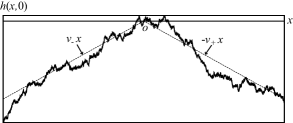
Figure 1: Two-sided Brownian motion initial condition with drifts $v_{\pm}$

The macroscopic shape of the height $h(x,t)$ for large $t$ is obtained by solving (1.1) where only the nonlinear term is taken into account and other terms (the diffusion and noise terms) are ignored. For the initial condition (2.1), it becomes

$$\frac{\lambda}{2\nu}h(x,t)=\begin{cases}\alpha^{2}v_{-}x+\nu\alpha^{4}v_{-}^{2}t&~{}\text{for~{}}x\leq-2\nu v_{-}\alpha^{2}t\\ -\frac{x^{2}}{4\nu t}&~{}\text{for~{}}\ -2\nu v_{-}\alpha^{2}t\leq x\leq 2\nu v_{+}\alpha^{2}t\\ -\alpha^{2}v_{+}x+\nu\alpha^{4}v_{+}^{2}t&~{}\text{for~{}}2\nu v_{+}\alpha^{2}t\leq x,\end{cases}$$ (2.2)

where $\alpha$ is given below (1.3). We are interested in the fluctuation property near the origin $x=0$ around this macroscopic profile. From the KPZ scaling, one expects that the fluctuation of the height scales like $O(t^{1/3})$ and nontrivial correlations are seen in the $x$ direction with scale $O(t^{2/3})$ when $t$ is large. Let us define a parameter $\gamma_{t}$ which scales as $O(t^{1/3})$ and a rescaled space coordinate $X$ by

$$\gamma_{t}=\left(\alpha^{4}\nu t\right)^{\frac{1}{3}},~{}~{}x=\frac{2\gamma_{t}^{2}X}{\alpha^{2}}.$$ (2.3)

We can introduce the scaled height $H_{t}(X)$ by

$$\frac{\lambda}{2\nu}h\left(\frac{2\gamma_{t}^{2}X}{\alpha^{2}},t\right)=-\frac{\gamma_{t}^{3}}{12}-\gamma_{t}X^{2}+\gamma_{t}H_{t}(X).$$ (2.4)

Here the term $-\gamma_{t}X^{2}$ in RHS comes from the parabolic profile (the middle equation) in (2.2). Let us define the probability distribution of $H_{t}(X)$,

$${F}_{v_{+},v_{-},t}(s;X)=\text{Prob}\left(\frac{\lambda}{2\nu}{h}\left(\frac{2\gamma_{t}^{2}X}{\alpha^{2}},t\right)+\frac{\gamma_{t}^{3}}{12}+\gamma_{t}X^{2}\leq\gamma_{t}s\right)=\text{Prob}({H}_{t}(X)\leq s).$$ (2.5)

In order to get an exact expression for this quantity, we now introduce the generalized height $\tilde{h}(x,t)$ defined by

$$\tilde{h}(x,t)=h(x,t)+\chi,$$ (2.6)

where the initial height of the overall surface $\chi$ is set to be a random variable such that $e^{\chi}$ obeys the inverse gamma distribution with parameter $v_{+}+v_{-}$, i.e. the probability density function of $e^{\chi}$ is given by

$$p(x)=\frac{1}{\Gamma{(v_{+}+v_{-})}}x^{-(v_{+}+v_{-})-1}e^{-\frac{1}{x}}{\bf{1}}_{x\geq 0}.$$ (2.7)

Although this definition (2.6) may look artificial, we will find that it has more tractable mathematical structure compared with $h(x,t)$ itself (see Proposition 1 below and Sec. 4.2). We also define the probability distribution $\tilde{F}_{v_{+},v_{-},t}(s;X)$ in a similar way to (2.5)

$$\tilde{F}_{v_{+},v_{-},t}(s;X)=\text{Prob}\left(\frac{\lambda}{2\nu}\tilde{h}\left(\frac{2\gamma_{t}^{2}X}{\alpha^{2}},t\right)+\frac{\gamma_{t}^{3}}{12}+\gamma_{t}X^{2}\leq\gamma_{t}s\right)=\text{Prob}({H}_{t}(X)+\frac{\lambda\chi}{2\nu\gamma_{t}}\leq s).$$ (2.8)

Our result for ${F}_{v_{+},v_{-},t}(s;X)$ and $\tilde{F}_{v_{+},v_{-},t}(s;X)$ are summarized as follows.

Proposition 1

$$F_{v_{+},v_{-},t}(s)=\frac{\Gamma(v_{+}+v_{-})}{\Gamma(v_{+}+v_{-}+\gamma_{t}^{-1}d/ds)}\tilde{F}_{v_{+},v_{-},t}(s),$$ (2.9)

$$\tilde{F}_{v_{+},v_{-},t}(s;X)=1-\int_{-\infty}^{\infty}due^{-e^{\gamma_{t}(s-u)}}g_{\gamma_{t}}(u;X).$$ (2.10)

Here $g_{\gamma_{t}}(u;X)$ is expressed as a difference of two Fredholm determinants,

$$g_{\gamma_{t}}(u;X)=\det\left(1-P_{u}(B^{\Gamma}_{\gamma_{t}}-P^{\Gamma}_{{\rm Ai}})P_{u}\right)-\det\left(1-P_{u}B^{\Gamma}_{\gamma_{t}}P_{u}\right),$$ (2.11)

where $P_{u}$ is a projection operator on $(u,\infty)$, and

$$B^{\Gamma}_{\gamma_{t}}(\xi_{1},\xi_{2})=\int_{0}^{\infty}dy{\rm Ai}_{\Gamma}^{\Gamma}\left(\xi_{1}+y,\frac{1}{\gamma_{t}},v_{+}-\frac{X}{\gamma_{t}},v_{-}+\frac{X}{\gamma_{t}}\right){\rm Ai}_{\Gamma}^{\Gamma}\left(\xi_{2}+y,\frac{1}{\gamma_{t}},v_{-}+\frac{X}{\gamma_{t}},v_{+}-\frac{X}{\gamma_{t}}\right)$$

$$+\int_{0}^{\infty}dy\frac{1}{e^{\gamma_{t}y}-1}\left[{\rm Ai}_{\Gamma}^{\Gamma}\left(\xi_{1}+y,\frac{1}{\gamma_{t}},v_{+}-\frac{X}{\gamma_{t}},v_{-}+\frac{X}{\gamma_{t}}\right){\rm Ai}_{\Gamma}^{\Gamma}\left(\xi_{2}+y,\frac{1}{\gamma_{t}},v_{-}+\frac{X}{\gamma_{t}},v_{+}-\frac{X}{\gamma_{t}}\right)\right.$$

$$\hskip 79.6678pt\left.-{\rm Ai}_{\Gamma}^{\Gamma}\left(\xi_{1}-y,\frac{1}{\gamma_{t}},v_{+}-\frac{X}{\gamma_{t}},v_{-}+\frac{X}{\gamma_{t}}\right){\rm Ai}_{\Gamma}^{\Gamma}\left(\xi_{2}-y,\frac{1}{\gamma_{t}},v_{-}+\frac{X}{\gamma_{t}},v_{+}-\frac{X}{\gamma_{t}}\right)\right],$$ (2.12)

$$P^{\Gamma}_{{\rm Ai}}(\xi_{1},\xi_{2})={\rm Ai}_{\Gamma}^{\Gamma}\left(\xi_{1},\frac{1}{\gamma_{t}},v_{+}-\frac{X}{\gamma_{t}},v_{-}+\frac{X}{\gamma_{t}}\right){\rm Ai}_{\Gamma}^{\Gamma}\left(\xi_{2},\frac{1}{\gamma_{t}},v_{-}+\frac{X}{\gamma_{t}},v_{+}-\frac{X}{\gamma_{t}}\right),$$ (2.13)

and the deformed Airy function ${\rm Ai}_{\Gamma}^{\Gamma}(a,b,c,d)$ is defined by

$${\rm Ai}_{\Gamma}^{\Gamma}(a,b,c,d)=\frac{1}{2\pi}\int_{\Gamma_{i\frac{d}{b}}}dze^{iza+i\frac{z^{3}}{3}}\frac{\Gamma\left(ibz+d\right)}{\Gamma\left(-ibz+c\right)}.$$ (2.14)

Here $\Gamma_{z_{p}}$ represents the contour from $-\infty$ to $\infty$ and, along the way, passing below the pole $z_{p}=id/b$.

We obtained this result by the replica method. The details of this approach and the derivation of Proposition 1 will be explained in Secs. 3 and 4. In (2.9), the factor $\frac{\Gamma(v_{+}+v_{-})}{\Gamma(v_{+}+v_{-}+\gamma_{t}^{-1}d/ds)}$ comes from the Laplace transform of the pdf of $e^{\chi}$ and is defined by the Taylor expansion. This equation represents the relation between ${F}_{v_{+},v_{-},t}(s;X)$ and $\tilde{F}_{v_{+},v_{-},t}(s;X)$, which will be discussed particularly in Sec. 4.2.

Note that the distribution function (2.10) is expressed as the convolution of the Gumbel distribution and the Fredholm determinants. Such a mathematical structure is common to the cases of the narrow wedge initial condition i.e. $h(x,0)=-|x|/\delta,~{}\delta\rightarrow 0$ [18, 19, 20, 21] and the half Brownian motion initial condition, i.e. $h(x,0)$ is BM for $x>0$ while the narrow wedge for $x<0$ [25, 36]. (This is the reason why we introduce the generalized height (2.6).) Moreover, (2.10) can be regarded as a generalization of the probability distributions for the narrow wedge and half-BM initial conditions: Noticing the relations

$$~{}\lim_{\begin{subarray}{c}v_{+}\rightarrow\infty\\ v_{-}\rightarrow\infty\end{subarray}}{\rm Ai}_{\Gamma}^{\Gamma}\left(x,\frac{1}{\gamma_{t}},v_{+}-\frac{X}{\gamma_{t}},v_{-}+\frac{X}{\gamma_{t}}\right){\rm Ai}_{\Gamma}^{\Gamma}\left(y,\frac{1}{\gamma_{t}},v_{-}+\frac{X}{\gamma_{t}},v_{+}-\frac{X}{\gamma_{t}}\right)={\rm Ai}(x){\rm Ai}(y),$$ (2.15)

$$~{}\lim_{\begin{subarray}{c}v_{+}\rightarrow 0\\ v_{-}\rightarrow\infty\end{subarray}}{\rm Ai}_{\Gamma}^{\Gamma}\left(x,\frac{1}{\gamma_{t}},v_{+}-\frac{X}{\gamma_{t}},v_{-}+\frac{X}{\gamma_{t}}\right){\rm Ai}_{\Gamma}^{\Gamma}\left(y,\frac{1}{\gamma_{t}},v_{-}+\frac{X}{\gamma_{t}},v_{+}-\frac{X}{\gamma_{t}}\right)$$

$$={\rm Ai}_{\Gamma}\left(x,\frac{1}{\gamma_{t}},-\frac{X}{\gamma_{t}}\right){\rm Ai}^{\Gamma}\left(y,\frac{1}{\gamma_{t}},-\frac{X}{\gamma_{t}}\right),$$ (2.16)

where

$${\rm Ai}_{\Gamma}(a,b,c)=\frac{1}{2\pi}\int_{-\infty}^{\infty}dze^{iza+i\frac{z^{3}}{3}}\frac{1}{\Gamma\left(-ibz+c\right)},$$ (2.17)

$${\rm Ai}^{\Gamma}(a,b,c)=\frac{1}{2\pi}\int_{\Gamma_{i\frac{c}{b}}}dze^{iza+i\frac{z^{3}}{3}}{\Gamma\left(ibz+c\right)},$$ (2.18)

we easily find the function (2.10) becomes that for the narrow wedge case as both $v_{+}$ and $v_{-}$ go to infinity and that for the half Brownian motion case as $v_{-}$ ($v_{+}$) goes to infinity (0).

2.1.2 Stationary limit

Here we consider the stationary limit where both drifts $v_{\pm}$ in (2.1) go to 0. When we take this limit for the expression (2.9), we notice that the Gamma function factor $\Gamma(v_{+}+v_{-})$ in (2.9) becomes divergent while the factor $\tilde{F}_{v_{+},v_{-},t}(s)$ vanishes since the term $\chi$ in (2.6) diverges. Thus we have to analyze carefully the limiting behavior of each factor, which will be discussed in Sec. 5. We obtain the following result: Let us introduce the scaled drifts $\omega_{\pm}=v_{\pm}/\gamma_{t}$ and consider the quantity $F_{w,t}(s)$ defined by

$$F_{w,t}(s;X)=\lim_{\begin{subarray}{c}\omega_{-}\rightarrow-\omega_{+}\\ \omega_{+}=w\end{subarray}}F_{{\omega_{+}}/{\gamma_{t}},{\omega_{-}}/{\gamma_{t}},t}(s;X).$$ (2.19)

Note that the situation $\omega_{+}+\omega_{-}=0$ corresponds to the case of flat macroscopic profile (see Fig. 1 and (2.2)) and the parameter $w$ determines the slope of the surface. The case $w=0$ corresponds to the initial condition (1.3). In terms of the functions

$$B_{a,b,u}(x):=\frac{e^{a^{3}/3-(x+u)a}}{\Gamma\left(\frac{a+b}{\gamma_{t}}+1\right)}-\int_{0}^{\infty}d\lambda e^{a\lambda}{\rm Ai}_{\Gamma}^{\Gamma}\left(x+u+\lambda,\frac{1}{\gamma_{t}},1+\frac{b}{\gamma_{t}},1+\frac{a}{\gamma_{t}}\right),$$ (2.20)

$$C_{t}(x):=\frac{e^{\gamma_{t}x}}{e^{\gamma_{t}x}-1}.$$ (2.21)

$F_{w,t}(s;X)$ is written as follows.

Theorem 2

$$F_{w,t}(s;X)=\frac{d/ds}{\Gamma(1+\gamma_{t}^{-1}d/ds)}\int_{-\infty}^{\infty}due^{-e^{\gamma_{t}(s-u)}}\left(\nu_{w,t}(u;X)-\nu_{w,t}^{(\delta)}(u;X)\right).$$ (2.22)

Here $\nu_{w,t}(u;X)$ and $\nu_{w,t}^{(\delta)}(u;X)$ are given by

$${\nu}_{w,t}(u;X)=\det\left(1-A_{w-X,-w+X}\right)L_{w-X,-w+X}(u)+\det\left(1-A_{w-X,-w+X}-D_{w-X,-w+X}\right),$$ (2.23)

$${\nu}_{w,t}^{(\delta)}(u;X)=\det\left(1-A^{(\delta)}_{w-X,-w+X}\right)L^{(\delta)}_{w-X,-w+X}(u)+\det\left(1-A^{(\delta)}_{w-X,-w+X}-D^{(\delta)}_{w-X,-w+X}\right),$$ (2.24)

respectively. The kernels $A_{a,b},~{}L_{a,b}$ and the function $D_{a,b}$ are represented as

$$A_{a,b}(\xi_{1},\xi_{2})$$

$$=C_{t}(\xi_{1})\int_{u}^{\infty}dy{\rm Ai}_{\Gamma}^{\Gamma}\left(\xi_{1}+y,\frac{1}{\gamma_{t}},1+\frac{b}{\gamma_{t}},1+\frac{a}{\gamma_{t}}\right){\rm Ai}_{\Gamma}^{\Gamma}\left(\xi_{2}+y,\frac{1}{\gamma_{t}},1+\frac{a}{\gamma_{t}},1+\frac{b}{\gamma_{t}}\right),$$ (2.25)

$$L_{a,b}(u)=\frac{1-a-b}{a+b}-\int_{-\infty}^{\infty}dxC_{t}(x)B_{a,b,u}(x)B_{b,a,u}(x),$$ (2.26)

$$D_{a,b}(\xi_{1},\xi_{2})=\left(A_{a,b}C_{t}B_{a,b,u}\right)(\xi_{1})B_{b,a,u}(\xi_{2})$$ (2.27)

where the functions $A^{(\delta)}_{a,b}$, $L^{(\delta)}_{a,b}$ and $D^{(\delta)}_{a,b}(u)$ are also defined in the same way as (2.25), (2.26) and (2.27) respectively with $C_{t}(x)$ (2.21) replaced by $C_{t}^{(\delta)}(x):=\frac{e^{\gamma_{t}x}}{e^{\gamma_{t}x}-1}-\delta(x)$.

Although in the limit $b\rightarrow-a$, the first term in (2.26) becomes divergent, we find the second term compensates for the divergence and obtain the following expression for (2.26),

$$L_{a,-a}(u) =-\frac{2\gamma}{\gamma_{t}}+u-a^{2}-1+\int_{-\infty}^{\infty}dxC_{t}(x)\left(B_{-a,a,u}^{(1)}(x)B_{a,-a,u}^{(2)}(x)+B_{a,-a,u}^{(1)}(x)B_{-a,a,u}^{(2)}(x)\right)$$

$$~{}~{}-\int_{-\infty}^{\infty}dxC_{t}(x)B_{a,-a,u}^{(2)}(x)B_{-a,a,u}^{(2)}(x),$$ (2.28)

where $\gamma$ is Euler’s constant and

$$B_{a,b,u}^{(1)}(x)=\frac{e^{a^{3}/3-(x+u)a}}{\Gamma\left(\frac{a+b}{\gamma_{t}}+1\right)},$$

$$B_{a,b,u}^{(2)}(x)=\int_{0}^{\infty}d\lambda e^{a\lambda}{\rm Ai}_{\Gamma}^{\Gamma}\left(x+u+\lambda,\frac{1}{\gamma_{t}},1+\frac{b}{\gamma_{t}},1+\frac{a}{\gamma_{t}}\right)$$ (2.29)

are the first and second term in (2.20).

The expression in Theorem 2 is suitable for numerical evaluations of the distribution function. By contrast Proposition 1 is not because we need precise estimations for both the divergence of the Gamma function factor and the convergence of the factor $\tilde{F}_{v_{+},v_{-},t}(s;X)$ to zero in the stationary limit. Fig. 2 shows the pictures of the probability density function for $w=X=0$. These are obtained by discretizing simply the Fredholm determinants in (2.23) and (2.24), which is sufficient for our purpose of getting those pictures. A more elaborate approximation technique for a Fredholm determinant has been developed recently in [49, 50, 51]. For accurate estimations of statistical quantities of our height distributions, this technique would be useful.

The distribution function obtained in this paper appears not merely in the KPZ equation but also in some time regime in various stochastic models [24, 27, 28]. One typical example is the asymmetric simple exclusion process (ASEP). The ASEP is a stochastic many-particle system where each particle hops to the right (left) neighboring site with rate $q$ ($p$) but it cannot hop to the occupied sites, which leads to the exclusion effect. Now we consider the ASEP on the one dimensional lattice $\mathbb{Z}$ and assume that at $t=0$, particles obey the two-sided Bernoulli initial condition with density $1/2$, where a particle occupy each site with probability $1/2$. Note that such a Bernoulli product measure is a stationary state of the ASEP. Let $N(x,t)$ be the (integrated) particle current i.e. difference between the numbers of the particles which pass from the site $x$ to the site $x+1$ and from the site $x+1$ to the site $x$ up to time $t$.

In [24], it was shown that

$$\lim_{\epsilon\rightarrow 0}\sqrt{\epsilon}\left(2N(\epsilon^{-1}x,\epsilon^{-2}t)+t\epsilon^{-3/2}/2\right)=h_{\frac{1}{2},1,1}(x,t)+\frac{t}{24}$$ (2.30)

where $\epsilon:=q-p$ is the difference between the right ($q$) and the left ($p$) hopping rates. The function $h_{\frac{1}{2},1,1}(x,t)$ is the (Cole-Hopf) solution to the KPZ equation with parameters $\nu=1/2,~{}\lambda=1,~{}D=1$ and with the initial condition given in (2.1) with $v_{+}=v_{-}=0$. This relation indicates that the height of the KPZ equation well approximates the current in the ASEP with the asymmetry $q-p$ being small, which is called the weakly ASEP (WASEP). Moreover it has been known recently that the KPZ equation also describes the dynamics of many other weakly driven growth processes in some time regime [27, 28]. The dots in Fig. 2 represent the Monte Carlo simulation for the particle current fluctuation $\sqrt{\epsilon}\left(2N(0,\epsilon^{-2}t)+t\epsilon^{-3/2}/2\right)$ for the WASEP with the two-sided Bernoulli initial condition mentioned above.

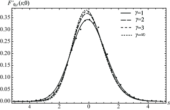
Figure 2: The probability density function of the height in the stationary situation $dF_{w=0,t}(s;X=0)/ds$ for $\gamma_{t}=1,2,3$. The dashed curve is $dF_{0}(s;0)/ds$. The dots ($\cdot$) indicate the Monte Carlo simulation for current distribution for the WASEP. We set the right hopping rate $q=0.575$ and the left rate $p=0.425$. (i.e. $\epsilon=q-p=0.15$), $3951$ Monte Carlo steps (corresponding to $\gamma_{t}=1$), and 10000 samples.

2.1.3 Long-time limit

We can also obtain the long-time limit of the height distribution function. We define $F_{w}(s;X)$ as $\lim_{t\rightarrow\infty}F_{w,t}(s;X)$ and obtain the following result.

Theorem 3

$$F_{w}(s;X)=\frac{d}{ds}\nu_{w}(s;X).$$ (2.31)

where $\nu_{w}(s;X):=\lim_{t\rightarrow\infty}\nu_{w,t}(s;X)$ has the following expression.

$$\nu_{w}(s;X)=\det\left(1-\mathcal{A}\right)\mathcal{L}_{w-X,-w+X}(s)+\det\left(1-\mathcal{A}-\mathcal{D}_{w-X,-w+X}\right).$$ (2.32)

Here $\mathcal{A}$, $\mathcal{D}_{a,b}$ and $\mathcal{L}_{a,b}$ are the long-time limit of $A_{a,b}$, $D_{a,b}$ and $L_{a,b}$ defined in Theorem 2 and are given by

$$\mathcal{A}(x,y)=P_{0}(x)\int_{u}^{\infty}d\xi{\rm Ai}(x+\xi){\rm Ai}(y+\xi),$$ (2.33)

$$\mathcal{L}_{a,b}(s)=\frac{1-a-b}{a+b}-\int_{0}^{\infty}dx\mathcal{B}_{a,s}(x)\mathcal{B}_{b,s}(x),$$ (2.34)

$$\mathcal{D}_{a,b}(x,y)=\left(\mathcal{A}P_{0}\mathcal{B}_{a,s}\right)(x)\mathcal{B}_{b,s}(y),$$ (2.35)

$$\mathcal{B}_{a,s}(x)=e^{\frac{a^{3}}{3}-(x+s)a}-\int_{0}^{\infty}d\lambda e^{a\lambda}{\rm Ai}(x+s+\lambda).$$ (2.36)

Note that $\det\left(1-\mathcal{A}\right)$ in (2.32) is nothing but the GUE Tracy-Widom distribution. The expression for $\mathcal{L}_{a,-a}$ corresponding to (2.28) is given by

$$\mathcal{L}_{a,-a}(s)=s-a^{2}-1+\int_{s}^{\infty}dx\left(\mathcal{B}_{-a,s}^{(1)}(x)\mathcal{B}_{a,s}^{(2)}(x)+\mathcal{B}_{a,s}^{(1)}(x)\mathcal{B}_{-a,s}^{(2)}(x)\right)-\int_{s}^{\infty}dx\mathcal{B}_{a,s}^{(2)}(x)\mathcal{B}_{-a,s}^{(2)}(x),$$ (2.37)

where $\mathcal{B}_{a,s}^{(1)}(x)$ ($\mathcal{B}_{a,s}^{(2)}(x)$) represents the first (second) term in (2.36), i.e.

$$\mathcal{B}_{a,s}^{(1)}(x)=e^{\frac{a^{3}}{3}-(x+s)a},~{}~{}\mathcal{B}_{a,s}^{(2)}(x)=\int_{0}^{\infty}d\lambda e^{a\lambda}{\rm Ai}(x+s+\lambda).$$ (2.38)

This function $F_{w}(s)$ has already appeared as a limiting distribution for other stochastic processes such as the PNG model [7] and the TASEP [46] in stationary situation. This implies that $F_{w}(s;X)$ appears commonly in the stationary subclass in the KPZ universality. Our result above is a representation which does not include any resolvent kernel such as $(1-\mathcal{A})^{-1}(x,y)$ thus it is convenient for numerical calculation. In Fig. 2, we also depicted the picture for the long-time limit using (2.22).

The derivation of the above theorem will be provided in Sec. 6.

2.2 The two-point correlation functions

The two-point function of the height is defined as

$$C(x,t)=\left\langle(h(x,t)-\langle h(x,t)\rangle)^{2}\right\rangle.$$ (2.39)

Considering the scaling property (2.4), we also introduce the scaling form

$$g_{t}(y)=2^{-4/3}\left(\frac{\lambda}{2\nu\gamma_{t}}\right)^{2}C\left(2^{1/3}\frac{2\gamma_{t}^{2}}{\alpha^{2}}y,t\right)$$ (2.40)

where we put the overall factor $2^{-4/3}$ and the factor $2^{1/3}$ in the argument of $C(x,t)$ following the convention in [45].

Moreover the two-point function of the slope of the height $\left\langle\partial_{x}h(0,0)\partial_{x}h(x,t)\right\rangle$ is also an important quantity since the height slope $\partial_{x}h(x,t)$ corresponds to the particle density in the interacting particle processes such as the ASEP. It has been pointed out in [45] that this is expressed as the second derivative of $C(x,t)$,

$$\left\langle\partial_{x}h(0,0)\partial_{x}h(x,t)\right\rangle=\frac{1}{2}\partial_{x}^{2}C(x,t)$$ (2.41)

Thus we are also interested in the second derivative of the scaling function $g^{\prime\prime}_{t}(y)$.

Noting that (2.39) is just the variance of $h(x,t)$, we readily obtain the following result for $g_{t}(y)$:

Corollary 4

$$g_{t}(y)=2^{-4/3}\left(\int_{-\infty}^{\infty}s^{2}\frac{dF_{w=0,t}(s;2^{1/3}y)}{ds}ds-\left(\int_{-\infty}^{\infty}s\frac{dF_{w=0,t}(s;2^{1/3}y)}{ds}ds\right)^{2}\right)$$ (2.42)

where $F_{w,t}(s;X)$ is given in (2.22).

Fig. 3 shows the function $g^{\prime\prime}_{t}(y)$ for $\gamma_{t}=1,2,3$. The dots in this figure correspond to the Monte Carlo simulation of density correlation in the WASEP

$$\langle\eta_{x,t}\eta_{0,0}\rangle_{\text{WASEP}}-1/4$$ (2.43)

where $\eta_{x,t}$ is the occupation variable. i.e. if the site $x$ is occupied (empty) at time $t$, $\eta_{x,t}=1~{}(0)$ and $\langle~{}~{}\rangle_{\text{WASEP}}$ means the averaging over both two-sided Bernoulli initial configuration and WASEP dynamics.

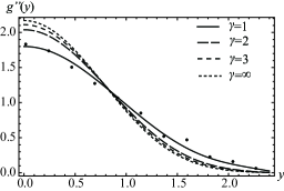
Figure 3: Stationary two-point correlation function $g_{t}^{\prime\prime}(y)$ for the KPZ equation for $\gamma_{t}=1,2,3$. The dashed curve represents the one in the scaling limit $g^{\prime\prime}(y)$. The dots indicates the Monte Carlo result of the WASEP, where parameters are the same as those in Fig. 2.

3 Replica analysis

3.1 Cole-Hopf solution, $\delta$-Bose gas

By the scaling of the KPZ equation, we find the height $h_{\nu,\lambda,D}(x,t)$ of the KPZ equation with general parameters $\nu,~{}\lambda,~{}D$ and $h_{\frac{1}{2},1,1}(x,t)$ with the specialized parameters $\nu=\frac{1}{2},\lambda=D=1,$ are related as

$$\frac{\lambda}{2\nu}h_{\nu,\lambda,D}\left(x,\frac{t}{2\nu}\right)=h_{\frac{1}{2},1,1}(\alpha^{2}x,\alpha^{4}t),$$ (3.1)

where $\alpha$ is defined below (1.3), for details see [36]. Thus in the following we concentrate on the height $h_{\frac{1}{2},1,1}(x,t)$ and omit the indices $\frac{1}{2},1,1$.

Applying the Cole-Hopf transformation,

$$Z(x,t)=e^{h(x,t)},$$ (3.2)

the KPZ equation (1.1) is linearized as

$$\frac{\partial Z(x,t)}{\partial t}=\frac{1}{2}\frac{\partial^{2}Z(x,t)}{\partial x^{2}}+\eta(x,t)Z(x,t),$$ (3.3)

which is called the stochastic heat equation. Now we would like to remark on the regularization of the KPZ equation. The KPZ equation (1.1) is in fact not well-defined due to the interplay between the nonlinear term and the singular property of the noise in (1.1). The typical regularization is to interpret (3.3) as Itô type and to define the regularized KPZ equation by the inverse Cole-Hopf transformation of (3.3). This is called the Cole-Hopf solution of the KPZ equation [24]. For more detailed discussion, see [36]. Recently a new way of regularization without using the Cole-Hopf transformation (3.2) was proposed in [52].

Eq. (3.3) can be interpreted as a problem of directed polymer in random media. Applying the Feynman path integral representation and taking the average with respect to $\eta$, we see the problem becomes that of the delta function Bose gas with attractive interaction,

$$H_{N}=-\frac{1}{2}\sum_{j=1}^{N}\frac{\partial^{2}}{\partial x_{j}^{2}}-\frac{1}{2}\sum_{j\neq k}^{N}\delta(x_{j}-x_{k}),$$ (3.4)

in terms of which the replica partition function $\langle Z^{N}(x,t)\rangle$ can be written as

$$\langle Z^{N}(x,t)\rangle=\langle x|e^{-H_{N}t}|\Phi\rangle.$$ (3.5)

Here $\langle x|$ represents the state with all $N$ particles being at the position $x$ and the $|\Phi\rangle$ the initial state of the $\delta$-function Bose gas. This is an important property of the replica approach to the KPZ equation [28, 29, 30]. The integrability of the Hamiltonian (3.4) allows us to calculate exactly the replica partition function.

One can perform the average over the initial distribution given by the two-sided Brownian motion and the dependence of $|\Phi\rangle$ on $x_{1},\ldots,x_{N}$ can be explicitly calculated as follows. First let us assume $x_{1}<x_{2}<\ldots<x_{N}$. For $x_{1}<\ldots<x_{l}<0<x_{l+1}<\ldots<x_{N},1\leq l\leq N$, one finds

$$\quad\langle x_{1},\cdots,x_{N}|\Phi\rangle$$

$$=\langle\exp\left[B_{-}(-x_{1})+\cdots+B_{-}(-x_{l})+B_{+}(x_{l+1})+\cdots+B_{+}(x_{N})\right]\rangle$$

$$=e^{v_{-}\sum_{j=1}^{l}x_{j}-v_{+}\sum_{j=l+1}^{N}x_{j}}\prod_{j=1}^{l}e^{-\frac{1}{2}(2l-2j+1)x_{l}}\prod_{k=1}^{N-l}e^{\frac{1}{2}(2(N-l-k)+1)x_{l+k}},$$ (3.6)

where $\langle~{}~{}\rangle$ denotes the averaging over BMs $B_{\pm}(x)$ (2.1) and in the last equality we used the property of BM, $\langle B(x)B(y)\rangle=\min(x,y)$. Since we are considering a Boson system, we symmetrize the function with respect to $x_{1},\ldots,x_{N}$ to have

$$\langle x_{1},\cdots,x_{N}|\Phi\rangle =\sum_{P\in S_{N}}e^{v_{-}\sum_{j=1}^{l}x_{P(j)}-v_{+}\sum_{j=l+1}x_{P(j)}}\prod_{j=1}^{l}e^{-\frac{1}{2}(2j-1)x_{P(j)}}$$

$$~{}~{}\times\prod_{k=1}^{N-l}e^{\frac{1}{2}(2(N-l-k)+1)x_{P(l+k)}}\prod_{j=1}^{N}\Theta\left(x_{P(j)}-x_{P(j-1)}\right).$$ (3.7)

Here $S_{N}$ denotes the set of permutations of order $N$, $\Theta(x)$ is the step function and we set $x_{P(0)}=0$.

The eigenvalues and eigenfunctions of the $\delta$-Bose gas can be constructed by using the Bethe ansatz [32, 33] (see also [30]). Let $|\Psi_{z}\rangle$ and $E_{z}$ be the eigenstate and its eigenvalue of $H_{N}$,

$$H_{N}|\Psi_{z}\rangle=E_{z}|\Psi_{z}\rangle.$$ (3.8)

By the Bethe ansatz, the eigenstate is given as

$$\langle x_{1},\cdots,x_{N}|\Psi_{z}\rangle=C_{z}\sum_{P\in S_{N}}{\text{sgn}P}\prod_{1\leq j<k\leq N}\left(z_{P(j)}-z_{P(k)}+i\text{sgn}(x_{j}-x_{k})\right)\exp\left(i\sum_{l=1}^{N}z_{P(l)}x_{l}\right)$$ (3.9)

where $C_{z}$ is the normalization constant, for which a formula is given in (3.11) below.

For the $\delta$-Bose gas with attractive interaction, the quasimomenta $z_{j}~{}(1\leq j\leq N)$, which label the state, are in general complex numbers. $z_{j}~{}(1\leq j\leq N)$ are divided into $M$ groups where $1\leq M\leq N$. The $\alpha$th group consists of $n_{\alpha}$ quasimomenta $z_{j}^{\prime}s$ which share the common real part $q_{\alpha}$. Note that $\sum_{\alpha=1}^{M}n_{\alpha}=N$. The quasimomenta in each group line up with regular intervals with unit length along the imaginary direction. Using $q_{\alpha}$ and $n_{\alpha}~{}(1\leq\alpha\leq M)$, we represent $z_{j}$ $(1\leq j\leq N)$ as

$$z_{j}=q_{\alpha}-\frac{i}{2}\left(n_{\alpha}+1-2r_{\alpha}\right),~{}~{}\text{for}~{}j=\sum_{\beta=1}^{\alpha-1}n_{\beta}+r_{\alpha},$$ (3.10)

where $1\leq\alpha\leq M$ and $1\leq r_{\alpha}\leq n_{\alpha}$. The normalization constant $C_{z}$ in (3.9), which is taken to be a positive real number, and the eigenvalue $E_{z}$ are given by [30]

$$C_{z} =\left(\frac{1}{N!}\prod_{\alpha=1}^{M}\frac{(n_{\alpha}!)^{2}}{n_{\alpha}}\prod_{1\leq j<k\leq N}\frac{1}{|z_{j}-z_{k}-i|^{2}}\right)^{1/2},$$ (3.11)

$$E_{z} =\frac{1}{2}\sum_{j=1}^{N}z_{j}^{2}=\frac{1}{2}\sum_{\alpha=1}^{M}n_{\alpha}q_{\alpha}^{2}-\frac{1}{24}\sum_{\alpha=1}^{M}\left(n_{\alpha}^{3}-n_{\alpha}\right).$$ (3.12)

The completeness of these states has been proved in [53, 54, 55].

The replica partition function $\langle Z^{N}(x,t)\rangle$ (3.5) can be written as

$$\langle Z^{N}(x,t)\rangle =\int_{-\infty}^{\infty}dy_{1}\cdots\int_{-\infty}^{\infty}dy_{N}\langle x|e^{-H_{N}t}|y_{1},\cdots,y_{N}\rangle\langle y_{1},\cdots,y_{N}|\Phi\rangle$$ (3.13)

Expanding the propagator $\langle x|e^{-H_{N}t}|y_{1},\cdots,y_{N}\rangle$ by the Bethe eigenstates of the $\delta$-Bose gas (3.9), we have

$$\langle Z^{N}(x,t)\rangle =\sum_{M=1}^{N}\frac{1}{M!}\prod_{j=1}^{N}\int_{-\infty}^{\infty}dy_{j}\left(\int_{-\infty}^{\infty}\prod_{\alpha=1}^{M}\frac{dq_{\alpha}}{2\pi}\sum_{n_{\alpha}=1}^{\infty}\right)\delta_{\sum_{\beta=1}^{M}n_{\beta},N}$$

$$\quad\times e^{-E_{z}t}\langle x|\Psi_{z}\rangle\langle\Psi_{z}|y_{1},\cdots,y_{N}\rangle\langle y_{1},\cdots,y_{N}|\Phi\rangle.$$ (3.14)

Now we want to perform the integrations over $y_{j},~{}(1\leq j\leq N)$ in this equation, Using (3.7) and noticing the symmetry of the eigenfunction (3.9), $\langle\Psi_{z}|y_{P(1)},\cdots,y_{P(N)}\rangle=\langle\Psi_{z}|y_{1},\cdots,y_{N}\rangle$, we find that RHS of (3.14) is represented as

$$\langle{Z}^{N}(x,t)\rangle =\sum_{M=1}^{N}\frac{N!}{M!}\sum_{\ell=0}^{N}\int_{y_{1}<\cdots<y_{\ell}<0<y_{\ell+1}<\cdots<y_{N}}dy_{1}\cdots dy_{N}\prod_{\alpha=1}^{M}\left(\int_{-\infty}^{\infty}\frac{dq_{\alpha}}{2\pi}\sum_{n_{\alpha}=1}^{\infty}\right)\delta_{\sum_{\beta=1}^{M}n_{\beta},N}$$

$$~{}\times e^{-E_{z}t}\langle x|\Psi_{z}\rangle\langle\Psi_{z}|y_{1},\cdots,y_{N}\rangle$$

$$\times e^{v_{-}\sum_{j=1}^{l}y_{j}-v_{+}\sum_{j=l+1}y_{j}}\prod_{j=1}^{l}e^{-\frac{1}{2}(2j-1)y_{j}}\prod_{k=1}^{N-l}e^{\frac{1}{2}(2(N-l-k)+1)y_{l+k}}.$$ (3.15)

Here we find the necessity of the drift terms in (2.1). Note that due to the factors $\exp(-\frac{1}{2}(2l-2j+1)y_{j})$ and $\exp(\frac{1}{2}(2(N-l-k)+1)$ we could not perform the integrations over $y_{k},~{}k=1,\cdots,N$ prior to those over $q_{\alpha},~{}\alpha=1,\cdots,M$ if we did not introduce the drifts $v_{\pm}$. Now we perform the integrations of $y_{j}~{}(1\leq j\leq N)$ by assuming that the drifts are positively large enough, which is the main reason why we introduced the drifts. Eq. (3.14) can now be expressed as

$$\langle{Z}^{N}(x,t)\rangle=\sum_{M=1}^{N}\frac{1}{M!}\prod_{\alpha=1}^{M}\left(\int_{-\infty}^{\infty}\frac{dq_{\alpha}}{2\pi}\sum_{n_{\alpha}=1}^{\infty}\right)\delta_{\sum_{\beta=1}^{M}n_{\beta},N}\langle x|\Psi_{z}\rangle\langle\Psi_{z}|\Phi\rangle e^{-E_{z}t}.$$ (3.16)

Here $\langle x|\Psi_{z}\rangle$ is given by (3.9) with $x_{1}=\cdots=x_{N}=x$ and $\langle\Psi_{z}|\Phi\rangle$ is computed as

$$~{}\langle\Psi_{z}|\Phi\rangle=\prod_{j=1}^{N}\int_{-\infty}^{\infty}dy_{j}\langle\Psi_{z}|y_{1},\cdots,y_{N}\rangle\langle y_{1},\cdots,y_{N}|\Phi\rangle$$

$$=N!C_{z}\sum_{P\in S_{N}}\text{sgn}P\left(z^{*}_{P(j)}-z^{*}_{P(k)}+i)\right)\sum_{l=0}^{N}\int_{y_{1}<\cdots<y_{l}<0}dy_{1}\cdots dy_{l}\prod_{m=1}^{l}e^{\left(-iz^{*}_{P(m)}+v_{-}-\frac{1}{2}(2m-1)\right)y_{m}}$$

$$\quad\times\int_{0<y_{l+1}<\cdots<y_{N}}dy_{l+1}\cdots dy_{N}\prod_{m=1}^{N-l}e^{\left(-iz^{*}_{P(l+m)}-v_{+}+\frac{1}{2}(2(N-l-m)+1)\right)y_{l+m}}$$

$$=(-1)^{N}N!C_{z}\sum_{P\in S_{N}}{\text{sgn}P}\prod_{1\leq j<k\leq N}\left(z^{*}_{P(j)}-z^{*}_{P(k)}+i\right)$$

$$\quad\times\sum_{l=0}^{N}(-1)^{l}\prod_{m=1}^{l}\frac{1}{\sum_{j=1}^{m}(-iz^{*}_{P{(j)}}+v_{-})-m^{2}/2}\prod_{m=1}^{N-l}\frac{1}{\sum_{j=N-m+1}^{N}(-iz^{*}_{P{(j)}}-v_{+})+m^{2}/2}.$$ (3.17)

Here we assume that $\sum_{j=1}^{m}(-iz^{*}_{P{(j)}}+v_{-})-m^{2}/2>0$ and $\sum_{j=N-m+1}^{N}(-iz^{*}_{P{(j)}}-v_{+})+m^{2}/2$ for any $m~{}(1\leq m\leq N)$. For example if we set $v_{\pm}>N/2+\max_{\alpha}n_{\alpha}/2$, the above conditions are satisfied.

3.2 Combinatorial identities

For further analysis of the integrand in (3.16), we need two combinatorial identities for $\langle x|\Psi_{z}\rangle$ and $\langle\Psi_{z}|\Phi\rangle$. The first one is for $\langle x|\Psi_{z}\rangle$. One has

$$\sum_{P\in S_{N}}{\text{sgn}P}\prod_{1\leq j<k\leq N}\left(w_{P(j)}-w_{P(k)}+if(j,k)\right)=N!\prod_{1\leq j<k\leq N}(w_{j}-w_{k})$$ (3.18)

for any complex variables $w_{j}$ $(1\leq j\leq N)$ and $f(j,k)$. This identity was derived as Lemma 1 in [37].

The next one for the term $\langle\Psi_{z}|\Phi\rangle$ is

Lemma 5 For any complex numbers $w_{j}~{}(1\leq j\leq N)$ and $a$,

$$~{}\sum_{P\in S_{N}}{\text{\rm sgn}P}\prod_{1\leq j<k\leq N}\left(w_{P(j)}-w_{P(k)}+a\right)$$

$$\quad\times\sum_{l=0}^{N}(-1)^{l}\prod_{m=1}^{l}\frac{1}{\sum_{j=1}^{m}(w_{P(j)}+v_{-})-m^{2}a/2}\prod_{m=1}^{N-l}\frac{1}{\sum_{j=N-m+1}^{N}(w_{P{(j)}}-v_{+})+m^{2}a/2}$$

$$~{}=\frac{\prod_{m=1}^{N}(v_{+}+v_{-}-am)\prod_{1\leq j<k\leq N}(w_{j}-w_{k})}{\prod_{m=1}^{N}(w_{m}+v_{-}-a/2)(w_{m}-v_{+}+a/2)}.$$ (3.19)

Proof

First we note that a similar identity,

$$\sum_{P\in S_{N}}{\text{\rm sgn}P}\prod_{1\leq j<k\leq N}\left(w_{P(j)}-w_{P(k)}+a\right)\prod_{m=1}^{N-l}\frac{1}{\sum_{j=N-m+1}^{N}w_{P(j)}+m^{2}a/2}=\frac{\prod_{1\leq j<k\leq N}(w_{j}-w_{k})}{\prod_{m=1}^{N}(w_{m}+a/2)},$$ (3.20)

which is the special case $v_{-}\rightarrow-\infty,~{}v_{+}\rightarrow 0$ of the above (3.19), was already proved in [36]. By using this identity for both terms with $v_{+}$ and $v_{-}$ on LHS, one can rewrite LHS of (3.19) as

$$\sum_{n=0}^{N}(-1)^{n}\sum_{\begin{subarray}{c}1\leq j_{1}<\ldots<j_{n}\leq N\\ 1\leq k_{1}<\ldots<k_{N-n}\leq N\\ \{j_{l}\}_{l=1}^{n}\cap\{k_{m}\}_{m=1}^{N-n}=\phi\end{subarray}}\text{sgn}S\prod_{1\leq l<l^{\prime}\leq n}(w_{j_{l}}-w_{j_{l^{\prime}}})\prod_{1\leq m<m^{\prime}\leq N-n}(w_{k_{m}}-w_{k_{m^{\prime}}})$$

$$\times\prod_{l=1}^{n}\prod_{m=1}^{N-n}(w_{j_{l}}-w_{k_{m}}+a)\prod_{l=1}^{n}\frac{1}{w_{j_{l}}+v_{-}-a/2}\prod_{m=1}^{N-n}\frac{1}{w_{k_{m}}-v_{+}+a/2}.$$ (3.21)

where $S=\{j_{1},\cdots,j_{n},k_{1},\cdots,k_{N-n}\}$. At this point we multiply both sides by $\prod_{m=1}^{N}(w_{m}+v_{-}-a/2)(w_{m}-v_{+}+a/2)$ and then set $v_{+}=a/2,v_{-}=b+a/2$ without losing the generality. Hence what we want to show is

$$\sum_{n=0}^{N}(-1)^{n}\sum_{\begin{subarray}{c}1\leq j_{1}<\ldots<j_{n}\leq N\\ 1\leq k_{1}<\ldots<k_{N-n}\leq N\\ \{j_{l}\}_{l=1}^{n}\cap\{k_{m}\}_{m=1}^{N-n}=\phi\end{subarray}}\text{sgn}S\prod_{1\leq l<l^{\prime}\leq n}(w_{j_{l}}-w_{j_{l^{\prime}}})\prod_{1\leq m<m^{\prime}\leq N-n}(w_{k_{m}}-w_{k_{m^{\prime}}})$$

$$\times\prod_{l=1}^{n}\prod_{m=1}^{N-n}(w_{j_{l}}-w_{k_{m}}+a)\prod_{l=1}^{n}w_{j_{l}}\prod_{m=1}^{N-n}(w_{k_{m}}+b)=\prod_{m=0}^{N-1}(b-am)\prod_{1\leq j<k\leq N}(w_{j}-w_{k}).$$ (3.22)

Here we prove this by noting that both sides can be considered as a polynomial in $a$ and $b$ and arguing by induction that the coefficients (which are polynomials of $\{w_{1},\ldots,w_{N}\}$) for each $b^{n}a^{m}$ in both sides are the same. First we observe that LHS is anti-symmetric with respect to $\{w_{1},\ldots,w_{N}\}$. Hence the coefficient $b^{n}a^{m}$ is also anti-symmetric with respect to $\{w_{1},\ldots,w_{N}\}$. Then all we should check is the numerical coefficients of terms $\prod_{j=1}^{N}w_{j}^{c_{j}}$ satisfying $c_{N}>\cdots>c_{1}\geq 0$. For instance when $N=2$, the equality we want to show reads

$$(w_{1}-w_{2})(w_{1}+b)(w_{2}+b)-(w_{1}-w_{2}+a)w_{1}(w_{2}+b)+(w_{2}-w_{1}+a)(w_{1}+b)w_{2}$$

$$+(w_{1}-w_{2})w_{1}w_{2}=b(b-a)(w_{1}-w_{2}).$$ (3.23)

We compare the coefficients of $1,a,b,ba,b^{2}$. For example for that for $b$, we see the coefficient of $w_{1}w_{2}^{2}$ is zero; for $ab$, we see the coefficient of $w_{2}$ is one.

To consider general $N$, we introduce a graphical representation. Each graph corresponds to each term in LHS of (3.22). First we put $n$ numbers $\{j_{1},\ldots,j_{n}\}$ to the left and $N-n$ numbers $\{k_{1},\ldots,k_{N-n}\}$ to the right. They are the vertices in a graph. Next if the term contains a factor from $w_{i}-w_{j}$ we draw a line joining $i$ and $j$ (edge); we also put circle on $i$ if the term contains $w_{i}$ and $j$ if $w_{j}$. In addition, if the term contains a factor coming from the last two products in LHS of (3.22), we encircle the number; hence we encircle all $j_{i}$’s. Finally by considering how each term can appear, we can put the sign to each graph. Because of the antisymmetry with respect to $\{w_{1},\cdots,w_{N}\}$, we need to list up only the graphs with $c_{N}>\cdots>c_{1}\geq 0$. The example of these graphs for $N=2,3$ are given in Figs. 4 (a) and (b) respectively. By looking at these graphs, one can confirm that there are several graphs which give non-zero contributions and all others give zero.

For showing the identity for general $N$, we use an induction. Suppose that we already showed the identity for $N$ by using the graphical representation. It consists of the several graphs corresponding to RHS of the identity (see e.g. the columns “$b^{3}$”, “$b^{2}a$” and “$ba^{2}$” in Fig. 4 (b)), where the corresponding coefficient is $\prod_{i=1}^{N}w_{i}^{i-1}$ up to sign, and all other graphs being grouped to vanish. Next we want to prove the identity for $N+1$. First notice that every graph which appears for $N+1$ is obtained by adding the vertex $N+1$ to some graph for $N$. If it is from a graph which can be grouped to vanish at $N$, then the term at $N+1$ can also be grouped to vanish. On the other hand, by adding $N+1$ to a graph corresponding to RHS of the identity at $N$, only four possible types of graphs at $N+1$ corresponding to the coefficient $\prod_{j=1}^{N+1}w_{j}^{c_{j}}$ with $c_{N+1}>c_{N}(=N-1)>c_{N-1}(=N-2)>\cdots>c_{2}(=1)>c_{1}(=0)$ can be produced. Fig. 4 (c) illustrates these four types. If we suppose the base graph at $N$ represents the coefficient $\prod_{j=2}^{N}w_{j}^{j-1}$ of $b^{n}a^{N-n}$, the types (i) and (ii) at $N+1$ (produced by adding the vertex $``N+1"$ to the base one) correspond to the coefficient $(-1)^{N+1}w^{N+1}\prod_{j=2}^{N}w_{j}^{j-1}$ and $(-1)^{N}w^{N+1}\prod_{j=2}^{N}w_{j}^{j-1}$ of $b^{n}a^{N-n}$ respectively, which cancel out each other. The types (iii) and (iv), on the other hand, correspond to the coefficient $(-1)^{N+1}\prod_{j=2}^{N+1}w_{j}^{j-1}$ of $b^{n}a^{N+1-n}$ and $(-1)^{N}\prod_{j=2}^{N+1}w_{j}^{j-1}$ of $b^{n+1}a^{N-n}$ respectively. Note also that in the type (iii), there are $N$ choices in total for connecting the vertex $N+1$ and the other ones with lines. Thus we find that for $m=0,1,\cdots,N$

$$C[b^{N+1-m}a^{m}]=(-1)^{N}w_{N+1}^{N}C[b^{N-m}a^{m}]+(-1)^{N-1}Nw_{N+1}^{N}C[b^{N-(m-1)}a^{m-1}],$$ (3.24)

where $C[b^{n}a^{m}]$ represents the coefficient of $b^{n}a^{m}$. This completes the proof. ∎

Figure 4: Graphical representations for the coefficient of each term in LHS of (3.22). (a) and (b) represents the case $N=2$ and $N=3$ respectively. In (c), we depict the possible four types of graph at $N-1$ which comes from the graph at $N$ corresponding to RHS of (3.22).

Using the identities (3.18) and (3.19) to (3.9) and (3.17) respectively, we get

$$\langle x|\Psi_{z}\rangle=N!C_{z}\prod_{1\leq j<k\leq N}(z_{j}-z_{k})e^{i\sum_{l=1}^{N}z_{l}x},$$ (3.25)

$$\langle\Psi_{z}|\Phi\rangle=N!C_{z}\prod_{1\leq j<k\leq N}(z^{*}_{j}-z^{*}_{k})\prod_{l=1}^{N}\frac{v_{+}+v_{-}-l}{(z^{*}_{l}+iv_{-}-i/2)(z^{*}_{l}-iv_{+}+i/2)}.$$ (3.26)

Thus using these relations and (3.11), we find that the factor $\langle x|\Psi_{z}\rangle\langle\Psi_{z}|\Phi\rangle$ in (3.16) becomes

$$\langle x|\Psi_{z}\rangle\langle\Psi_{z}|\Phi\rangle=N!\prod_{\alpha=1}^{M}\frac{(n_{\alpha}!)^{2}}{n_{\alpha}}\prod_{1\leq j<k\leq N}\frac{|z_{j}-z_{k}|^{2}}{|z_{j}-z_{k}-i|^{2}}\prod_{l=1}^{N}\frac{e^{iz_{l}x}(v_{+}+v_{-}-l)}{(-iz^{*}_{l}+v_{-}-1/2)(iz_{j}^{*}+v_{+}-1/2)},$$ (3.27)

We want to rewrite this equation in terms of $q_{\alpha}$ and $n_{\alpha}$ in (3.10). For the last factor of this equation, we easily find

$$\quad\prod_{l=1}^{N}\frac{e^{iz_{l}x}}{(-iz^{*}_{l}+v_{-}-1/2)(iz_{j}^{*}+v_{+}-1/2)}$$

$$=\prod_{\alpha=1}^{M}e^{in_{\alpha}q_{\alpha}x}\prod_{r=1}^{n_{\alpha}}\frac{1}{(-iq_{\alpha}+v_{-}+\frac{1}{2}(n_{\alpha}-2r))(iq_{\alpha}+v_{+}+\frac{1}{2}(n_{\alpha}-2r))}.$$ (3.28)

From (3.11) and (3.25), we know the remaining factors in (3.27) is represented by $|\langle 0|\Psi_{z}\rangle|^{2}$. For this quantity, the following result was obtained in Appendix B in [30],

$$|\langle 0|\Psi_{z}\rangle|^{2} =N!\prod_{\alpha=1}^{M}\frac{(n_{\alpha}!)^{2}}{n_{\alpha}}\prod_{1\leq j<k\leq N}\frac{|z_{j}-z_{k}|^{2}}{|z_{j}-z_{k}-i|^{2}}$$

$$=\frac{N!}{\prod_{\alpha=1}^{M}n_{\alpha}}\prod_{1\leq\alpha<\beta\leq M}\frac{|q_{\alpha}-q_{\beta}-\frac{i}{2}(n_{\alpha}-n_{\beta})|^{2}}{|q_{\alpha}-q_{\beta}-\frac{i}{2}(n_{\alpha}+n_{\beta})|^{2}}.$$ (3.29)

From (3.27)–(3.29), we get

$$\langle x|\Psi_{z}\rangle\langle\Psi_{z}|\Phi\rangle =N!\prod_{\ell=1}^{N}(v_{+}+v_{-}-\ell)\prod_{\alpha<\beta}^{M}\frac{|q_{\alpha}-q_{\beta}-\frac{i}{2}(n_{\alpha}-n_{\beta})|^{2}}{|q_{\alpha}-q_{\beta}-\frac{i}{2}(n_{\alpha}+n_{\beta})|^{2}}\prod_{\alpha=1}^{M}\frac{e^{in_{\alpha}q_{\alpha}x}}{n_{\alpha}}$$

$$~{}~{}\times\prod_{r=1}^{n_{\alpha}}\frac{1}{(-iq_{\alpha}+v_{-}+\frac{1}{2}(n_{\alpha}-2r))(iq_{\alpha}+v_{+}+\frac{1}{2}(n_{\alpha}-2r))}.$$ (3.30)

We can further deform (3.30) to an expression in terms of a determinant by using the Cauchy’s determinant formula,

$$\frac{\prod_{\alpha<\beta}^{M}(a_{\alpha}-a_{\beta})(b_{\alpha}-b_{\beta})}{\prod_{\alpha,\beta=1}^{M}(a_{\alpha}-b_{\beta})}=(-1)^{\frac{M(M-1)}{2}}\det\left(\frac{1}{a_{\alpha}-b_{\beta}}\right),$$ (3.31)

and a few basic properties of determinant. We find

$$\langle x|\Psi_{z}\rangle\langle\Psi_{z}|\Phi\rangle =2^{M}N!\prod_{\ell=1}^{N}(v_{+}+v_{-}-\ell)\det\left(\frac{1}{n_{j}+n_{k}+2i(q_{j}-q_{k})}\right)_{j,k=1}^{M}$$

$$~{}~{}\times\prod_{\alpha=1}^{M}e^{in_{\alpha}q_{\alpha}x}\prod_{r=1}^{n_{\alpha}}\frac{1}{(-iq_{\alpha}+v_{-}+\frac{1}{2}(n_{\alpha}-2r))(iq_{\alpha}+v_{+}+\frac{1}{2}(n_{\alpha}-2r))}$$

$$=2^{M}N!\prod_{\ell=1}^{N}(v_{+}+v_{-}-\ell)\prod_{\alpha=1}^{M}\left(\int_{0}^{\infty}d\omega_{\alpha}\right)\det\left(e^{-\omega_{j}(n_{j}+n_{k}+2i(q_{j}-q_{k}))}\right)_{j,k=1}^{M}$$

$$~{}~{}\times\prod_{\alpha=1}^{M}e^{in_{\alpha}q_{\alpha}x}\prod_{r=1}^{n_{\alpha}}\frac{1}{(-iq_{\alpha}+v_{-}+\frac{1}{2}(n_{\alpha}-2r))(iq_{\alpha}+v_{+}+\frac{1}{2}(n_{\alpha}-2r))}$$

$$=2^{M}N!\prod_{\ell=1}^{N}(v_{+}+v_{-}-\ell)\prod_{\alpha=1}^{M}\left(\int_{0}^{\infty}d\omega_{\alpha}\right)\det\left(K_{x}(n_{j},q_{j};\omega_{j},\omega_{k})\right)_{j,k=1}^{M},$$ (3.32)

where in the last equality, we used a simple fact

$$\det(a_{j}^{b_{j}+b_{k}})=\det((a_{j}a_{k})^{b_{j}}).$$ (3.33)

and the notation

$$~{}K_{x}(n_{j},q_{j};\omega_{j},\omega_{k})$$

$$:=e^{in_{j}q_{j}x-n_{j}(\omega_{j}+\omega_{k})-2iq_{j}(\omega_{j}-\omega_{k})}\prod_{r=1}^{n_{j}}\frac{1}{(-iq_{j}+v_{-}+\frac{1}{2}(n_{j}-2r))(iq_{j}+v_{+}+\frac{1}{2}(n_{j}-2r))}$$

$$=e^{in_{j}q_{j}x-n_{j}(\omega_{j}+\omega_{k})-2iq_{j}(\omega_{j}-\omega_{k})}\frac{\Gamma\left(-iq_{j}+v_{-}-\frac{n_{j}}{2}\right)\Gamma\left(iq_{j}+v_{+}-\frac{n_{j}}{2}\right)}{\Gamma\left(-iq_{j}+v_{-}+\frac{n_{j}}{2}\right)\Gamma\left(iq+v_{+}+\frac{n_{j}}{2}\right)}.$$ (3.34)

From (3.12), (3.16), and (3.32), we obtain an expression of $\langle Z^{N}(x,t)\rangle$ in terms of the determinant,

$$\quad\langle Z^{N}(x,t)\rangle e^{\frac{Nt}{24}+\frac{Nx^{2}}{2t}}$$

$$=\sum_{M=1}^{N}\frac{2^{M}N!}{M!}\prod_{\ell=1}^{N}(v_{+}+v_{-}-\ell)\prod_{\alpha=1}^{M}\left(\sum_{n_{\alpha}=1}^{\infty}\int_{-\infty}^{\infty}\frac{dq_{\alpha}}{2\pi}e^{-\frac{t}{2}n_{\alpha}q_{\alpha}^{2}+\frac{t}{24}n_{\alpha}^{3}}\int_{0}^{\infty}d\omega_{\alpha}\right)\delta_{\sum_{\beta=1}^{M}n_{\beta},N}$$

$$~{}\times\det\left(e^{n_{j}\frac{x^{2}}{2t}}K_{x}(n_{j},q_{j};\omega_{j},\omega_{k})\right)_{j,k=1}^{M}$$

$$=\sum_{M=1}^{N}\frac{N!}{M!}\prod_{\ell=1}^{N}(v_{+}+v_{-}-\ell)\prod_{\alpha=1}^{M}\left(\int_{0}^{\infty}d\omega_{\alpha}\sum_{n_{\alpha}=1}^{\infty}\right)\delta_{\sum_{\beta=1}^{M}n_{\beta},N}$$

$$\hskip 113.81102pt\times\det\left(\int_{-\infty}^{\infty}\frac{dq}{\pi}e^{n_{j}\frac{x^{2}}{2t}-\frac{t}{2}n_{j}q^{2}+\frac{t}{24}n_{j}^{3}}K_{x}(n_{j},q;\omega_{j},\omega_{k})\right)_{j,k=1}^{M}.$$ (3.35)

Here we would like to discuss the condition on the drifts $v_{\pm}$. In the above equation, we notice that the condition $v_{\pm}>N/2+\max_{\alpha}n_{\alpha}/2$ discussed below (3.17) ensures that all the poles $q=-i(v_{-}+(n_{j}/2-r)$ and $q=i(v_{+}-(n_{j}/2-r)$ with $~{}r=0,1,\cdots,n_{j}$ in the integrand $e^{n_{j}\frac{x^{2}}{2t}-\frac{t}{2}n_{j}q^{2}+\frac{t}{24}n_{j}^{3}}K_{x}(n_{j},q;\omega_{j},\omega_{k})$ lie on the lower and upper half plane respectively. Thus we can relax the condition to $v_{\pm}>\max_{\alpha}n_{\alpha}/2$, where the above property of the poles is retained.

4 Generating function and height distribution

4.1 Generating function

Now we define the generating function $G_{\gamma_{t}}(s;X)$ as

$$G_{\gamma_{t}}(s;X)=\sum_{N=0}^{\infty}\frac{\left(-e^{-\gamma_{t}s}\right)^{N}}{N!}\left\langle{Z}^{N}\left(2\gamma_{t}^{2}X,t\right)\right\rangle e^{N\frac{\gamma_{t}^{3}}{12}+N\gamma_{t}X^{2}}=\langle e^{-e^{\gamma_{t}(H_{t}(X)-s)}}\rangle,$$ (4.1)

where in the last equality, we used (2.4). Substituting (3.35) into this equation, we get

$$~{}G_{\gamma_{t}}(s;X)$$

$$=1+\sum_{N=1}^{\infty}\prod_{\ell=1}^{N}(v_{+}+v_{-}-\ell)\sum_{M=1}^{N}\frac{(-e^{-\gamma_{t}s})^{N}}{M!}\prod_{\alpha=1}^{M}\left(\int_{0}^{\infty}d\omega_{\alpha}\sum_{n_{\alpha}=1}^{\infty}\right)\delta_{\sum_{\beta=1}^{M}n_{\beta},N}$$

$$~{}\times\det\left(\int_{-\infty}^{\infty}\frac{dq}{\pi}e^{n_{j}\gamma_{t}X^{2}-\gamma_{t}^{3}n_{j}q^{2}+\frac{\gamma_{t}^{3}}{12}n_{j}^{3}}K_{2\gamma_{t}^{2}X}(n_{j},q;\omega_{j},\omega_{k})\right)_{j,k=1}^{M}.$$ (4.2)

4.2 Shifting

In the previous studies for the narrow-wedge [30, 28] and half Brownian motion initial condition [36], the generating functions corresponding to (4.2) were already described by the Fredholm determinant, which is an important achievement in the replica analyses. Unfortunately, however, this is not the case in (4.2) due to the factor $\prod_{j=1}^{N}(v_{+}+v_{-}-j)$. In order to resolve this problem, we introduced $\tilde{h}(x,t)$ in (2.6). Here we discuss some general properties of two random variables $h$ and $\tilde{h}$ related as

$$\tilde{h}=h+\chi,$$ (4.3)

where $\chi$ is also a random variable independent of $h$. Note that at this stage, $h$ and $\tilde{h}$ are just two random variables and do not have a specific meaning such as height. In addition, right now we do not assume a specific distribution for $\chi$. Let us define

$$Z=e^{h},~{}M(\xi)=\sum_{N=0}^{\infty}\frac{\langle(\xi h)^{N}\rangle}{N!}=\left\langle e^{\xi h}\right\rangle,~{}F(s)=\mathbb{P}[h\leq s].$$ (4.4)

and also $\tilde{Z},~{}\tilde{M}(\xi),~{}\tilde{F}(s)$ in the same way as (4.4) except that $h$ is replaced by $\tilde{h}$. We find that the following relation holds

$$\langle Z^{N}\rangle=\frac{1}{g(N)}\langle\tilde{Z}^{N}\rangle$$ (4.5)

$$M(\xi)=\frac{1}{g(\xi)}\tilde{M}(\xi),$$ (4.6)

and noticing the fact $\frac{dF(s)}{ds}=\int_{-\infty}^{\infty}d\xi M(i\xi)e^{-i\xi s},$ we also see

$$F(s)=\frac{1}{g(-\partial/\partial s)}\tilde{F}(s)$$ (4.7)

where $g(y)=\langle e^{y\chi}\rangle$.

In (2.6), we chose $\chi$ as the random variable such that $e^{\chi}$ obey the inverse gamma distribution with parameter $v_{+}+v_{-}$. The probability density function of the inverse gamma random variable is

$$p_{\theta}(x)=\frac{1}{\Gamma(\theta)}x^{-\theta-1}e^{-1/x}{\bf 1}_{x\geq 0},$$ (4.8)

where $\theta>0$ is a parameter and the function $g(\xi)$ in this case is given by

$$g(\xi)=\int_{0}^{\infty}x^{\xi}p_{\theta}(x)dx=\frac{1}{\Gamma(\theta)}\int_{0}^{\infty}x^{\xi-\theta-1}e^{-1/x}dx=\frac{\Gamma(\theta-\xi)}{\Gamma(\theta)}.$$ (4.9)

In particular, we notice that if we set $\theta=v_{+}+v_{-}$ as in (2.4), $g(N)$ becomes $1/\prod_{j=1}^{N}(v_{+}+v_{-}-j)$.

4.3 Generating function for the generalized height

We define $\tilde{Z}(x,t)$ and $\tilde{G}_{\gamma_{t}}(s;X)$ as (3.2) and (4.1) respectively with $h(x,t)$ replaced by $\tilde{h}(x,t)$. From the relation (4.5) and (4.9) with $\theta=v_{+}+v_{-}$, we see that $\langle\tilde{Z}^{N}(x,t)\rangle$ is related to $\langle Z^{N}(x,t)\rangle$ as

$$\langle\tilde{Z}^{N}(x,t)\rangle=\langle Z^{N}(x,t)\rangle\frac{1}{\prod_{j=1}^{N}(v_{+}+v_{-}-j)}.$$ (4.10)

Hence $\tilde{G}_{\gamma_{t}}(s;X)$ is calculated as

$$~{}\tilde{G}_{\gamma_{t}}(s;X):=\sum_{N=0}^{\infty}\frac{(-e^{-\gamma_{t}s})^{N}}{N!}\langle\tilde{Z}^{N}(2\gamma_{t}^{2}X,t)\rangle$$

$$=1+\sum_{N=1}^{\infty}\sum_{M=1}^{N}\frac{(-e^{-\gamma_{t}s})^{N}}{M!}\prod_{\alpha=1}^{M}\left(\int_{0}^{\infty}d\omega_{\alpha}\sum_{n_{\alpha}=1}^{\infty}\right)\delta_{\sum_{\beta=1}^{M}n_{\beta},N}$$

$$\hskip 142.26378pt\times\det\left(\int_{-\infty}^{\infty}\frac{dq}{\pi}e^{n_{j}\gamma_{t}X^{2}-\gamma_{t}^{3}n_{j}q^{2}+\frac{\gamma_{t}^{3}}{12}n_{j}^{3}}K_{2\gamma_{t}^{2}X}(n_{j},q;\omega_{j},\omega_{k})\right)_{j,k=1}^{M}$$

Note that this generating function does not include the term $\prod_{\ell=1}^{N}(v_{+}+v_{-}-\ell)$ in (4.2). In this case, we find the Fredholm determinant expression,

$$~{}\tilde{G}_{\gamma_{t}}(s;X)=\sum_{M=0}^{\infty}\frac{(-1)^{M}}{M!}\prod_{\alpha=1}^{M}\int_{0}^{\infty}d\omega_{\alpha}$$

$$\hskip 28.45274pt\times\det\left(\sum_{n=1}^{\infty}(-1)^{n-1}\int_{-\infty}^{\infty}\frac{dq}{\pi}e^{n_{j}\gamma_{t}X^{2}-\gamma_{t}^{3}n_{j}q^{2}+\frac{\gamma_{t}^{3}}{12}n_{j}^{3}-\gamma_{t}ns}K_{2\gamma_{t}^{2}X}(n,q;\omega_{j},\omega_{k})\right)_{j,k=1}^{M}.$$ (4.12)

Shifting the variable $q$ to $q+iX/\gamma_{t}$, we get

$$~{}\tilde{G}_{\gamma_{t}}(s;X)=\sum_{M=0}^{\infty}\frac{(-1)^{M}}{M!}\prod_{k=1}^{M}\int_{0}^{\infty}d\omega_{k}\det\left(K_{v_{+}-\frac{X}{\gamma_{t}},v_{-}+\frac{X}{\gamma_{t}}}(\omega_{j},\omega_{k})\right)_{j,k=1}^{M},$$ (4.13)

where the kernel $K_{v,w}(\omega_{j},\omega_{k})$ is written as

$$K_{v,w}(\omega_{j},\omega_{k}) =\sum_{n=1}^{\infty}(-1)^{n-1}\int_{-\infty}^{\infty}\frac{dq}{\pi}e^{-n(\omega_{j}+\omega_{k})-2iq(\omega_{j}-\omega_{k})-\gamma_{t}^{3}nq^{2}+\frac{\gamma_{t}^{3}}{12}n^{3}-\gamma_{t}ns}$$

$$\hskip 113.81102pt\times\frac{\Gamma\left(-iq+w-\frac{n}{2}\right)\Gamma\left(iq+v-\frac{n}{2}\right)}{\Gamma\left(-iq+w+\frac{n}{2}\right)\Gamma\left(iq+v+\frac{n}{2}\right)},$$ (4.14)

with $v,w>n/2$. In (4.13), we keep the contour of $q$ on the real axis by changing the condition for the drift to $v_{+}-X/\gamma_{t}>n/2,~{}v_{-}+X/\gamma_{t}>n/2$.

In the following, we provide another representation with the kernel using the deformed Airy functions ${\rm Ai}_{\Gamma}^{\Gamma}(a,b,c,d)$ defined in (2.14). We use the following two relations,

Lemma 6

(a) We set $q\in\mathbb{R}$ and  $m,~{}n\geq 0$. When $a,b>n/2$, we have

$$\frac{\Gamma\left(-iq+a-\frac{n}{2}\right)\Gamma\left(iq+b-\frac{n}{2}\right)}{\Gamma\left(-iq+a+\frac{n}{2}\right)\Gamma\left(iq+b+\frac{n}{2}\right)}e^{\frac{m^{3}n^{3}}{3}}=\int_{-\infty}^{\infty}dy{\rm Ai}_{\Gamma\Gamma}^{\Gamma\Gamma}\left(y,\frac{1}{2m},-iq+a,iq+b\right)e^{mny},$$ (4.15)

where

$${\rm Ai}_{\Gamma\Gamma}^{\Gamma\Gamma}\left(a,b,c,d\right)=\frac{1}{2\pi}\int_{\Gamma_{i\frac{c,d}{b}}}dze^{iaz+iz^{3}/3}\frac{\Gamma(ibz+c)\Gamma(ibz+d)}{\Gamma(-ibz+c)\Gamma(-ibz+d)}$$ (4.16)

with $\Gamma_{p}$ defined in (2.17) below.

(b) For $a,b,x\in\mathbb{R}$ and $w\geq 0$, we have

$$~{}\frac{1}{2\pi}\int_{-\infty}^{\infty}dp{\rm Ai}_{\Gamma\Gamma}^{\Gamma\Gamma}\left(p^{2}+v,w,-iwp+a,iwp+b\right)e^{ipx}$$

$$=\frac{1}{2^{\frac{1}{3}}}{\rm Ai}_{\Gamma}^{\Gamma}\left(2^{-\frac{2}{3}}(v+x),2^{\frac{1}{3}}w,a,b\right){\rm Ai}_{\Gamma}^{\Gamma}\left(2^{-\frac{2}{3}}(v-x),2^{\frac{1}{3}}w,b,a\right),$$ (4.17)

where ${\rm Ai}^{\Gamma}(a,b,c)$ and ${\rm Ai}_{\Gamma}(a,b,c)$ are defined by (2.18) and (2.17) respectively.

As will be discussed in Sec. 7, these relations (4.15) and (4.17) play a crucial role in the replica analysis. These are two-parameters ($a,b$) generalization of the ones used in the previous studies of half-Brownian motion [36] and the narrow wedge [28, 30] initial data: As either $a$ or $b$ goes to infinity in (4.15) and (4.17), they reproduce Lemma 6 (a) and (b) in [36] respectively. On the other hand, in the case where both $a$ and $b$ go to infinity, they converge to the ones appeared in [28, 30].

Proof

(a) RHS of (4.15) is written as

$$\frac{1}{2\pi}\int_{-\infty}^{\infty}dy\int_{\mathbb{R}+imn}dz\frac{\Gamma\left(i\frac{z}{2m}-iq+a\right)\Gamma\left(i\frac{z}{2m}+iq+b\right)}{\Gamma\left(-i\frac{z}{2m}-iq+a\right)\Gamma\left(-i\frac{z}{2m}+iq+b\right)}e^{i(z-imn)y+i\frac{z^{3}}{3}}.$$ (4.18)

Here we used the fact that the contour of $z$ can be deformed from to $\mathbb{R}+imn$ since the imaginary parts of the poles of the integrand $2m(ia-q+ir)$ and $2m(ib-q+ir)$, where $r=0,1,2,\cdots$ are larger than $mn$ when the condition $a,b>n/2$ is satisfied. In this equation, we change the variable $z$ on RHS to $y_{2}=z-imn$ and get

$$~{}\frac{1}{2\pi}\int_{-\infty}^{\infty}dy\int_{-\infty}^{\infty}d{y}_{2}\frac{\Gamma\left(-iq+a-\frac{n}{2}+i\frac{{y}_{2}}{2m}\right)\Gamma\left(iq+b-\frac{n}{2}+i\frac{{y}_{2}}{2m}\right)}{\Gamma\left(-iq+a+\frac{n}{2}-i\frac{{y}_{2}}{2m}\right)\Gamma\left(iq+b+\frac{n}{2}-i\frac{{y}_{2}}{2m}\right)}e^{iy{y}_{2}+i\frac{({y}_{2}+imn)^{3}}{3}}$$

$$=\int_{-\infty}^{\infty}d{y}_{2}\delta({y}_{2})\frac{\Gamma\left(-iq+a-\frac{n}{2}+i\frac{{y}_{2}}{2m}\right)\Gamma\left(iq+b-\frac{n}{2}+i\frac{{y}_{2}}{2m}\right)}{\Gamma\left(-iq+a+\frac{n}{2}-i\frac{{y}_{2}}{2m}\right)\Gamma\left(iq+b+\frac{n}{2}-i\frac{{y}_{2}}{2m}\right)}e^{i\frac{({y}_{2}+imn)^{3}}{3}}$$

$$=\frac{\Gamma\left(-iq+a-\frac{n}{2}\right)\Gamma\left(iq+b-\frac{n}{2}\right)}{\Gamma\left(-iq+a+\frac{n}{2}\right)\Gamma\left(iq+b+\frac{n}{2}\right)}e^{\frac{m^{3}n^{3}}{3}}.$$ (4.19)

(b) LHS of (4.17) reads

$$\frac{1}{(2\pi)^{2}}\int_{-\infty}^{\infty}dp\int_{\Gamma_{-p+i\frac{a,b}{w}}}dze^{i(p^{2}+v)z+i\frac{z^{3}}{3}+ipx}\frac{\Gamma\left(iw(z-p)+a\right)\Gamma\left(iw(z+p)+b\right)}{\Gamma\left(-iw(z+p)+a\right)\Gamma\left(-iw(z-p)+b\right)}.$$ (4.20)

By applying the change of variables $p=(z_{1}-z_{2})/2^{2/3}$ and $z=(z_{1}+z_{2})/2^{2/3}$, we obtain the desired expression. ∎

Applying (a) of the lemma with $a=v_{-}+X/\gamma_{t},b=v_{+}-X/\gamma_{t}$ and $m=\gamma_{t}/2^{2/3}$ to (4.14), one has

$$~{}~{}K_{v_{+}-\frac{X}{\gamma_{t}},v_{-}+\frac{X}{\gamma_{t}}}(\omega_{j},\omega_{k})$$

$$=\sum_{n=1}^{\infty}(-1)^{n-1}\int_{-\infty}^{\infty}\frac{dq}{\pi}\int_{-\infty}^{\infty}dy_{1}{\rm Ai}_{\Gamma\Gamma}^{\Gamma\Gamma}\left(y_{1},\frac{1}{2^{\frac{1}{3}}\gamma_{t}},-iq+v_{-}+\frac{X}{\gamma_{t}},iq+v_{+}-\frac{X}{\gamma_{t}}\right)e^{-2iq(\omega_{j}-\omega_{k})}$$

$$\hskip 142.26378pt\times e^{-n(\omega_{j}+\omega_{k}+\gamma_{t}^{3}q^{2}+\gamma_{t}s-2^{-\frac{2}{3}}\gamma_{t}y_{1})}.$$ (4.21)

So far we have imposed the condition for the drifts $v_{+}-X,v_{-}+X>n/2$ (see (4.13) and (4.14)). At this point, since RHS of (4.15) is well-defined for all $a,b\in\mathbb{R}$, we can relax it to the region such that the generalized height (2.6) under consideration is well-defined, i.e. $v_{+}+v_{-}>0$. Changing the variables $q,~{}\omega_{j}$ and $y_{1}$ to $p=2^{1/3}\gamma_{t}q,~{}\xi_{j}=2\gamma_{t}^{-1}\omega_{j}$ and $y=y_{1}/2^{2/3}-p^{2}/2^{2/3}-(\xi_{j}+\xi_{k})/2$, we see $K_{v_{+}-X/\gamma_{t},v_{-}+X/\gamma_{t}}(\omega_{j},\omega_{k})d\omega_{j}=\bar{K}_{v_{+}-X/\gamma_{t},v_{-}+X/\gamma_{t}}(\xi_{j},\xi_{k})d\xi_{j}$, where

$$\bar{K}_{v,w}(\xi_{j},\xi_{k}) =\frac{2^{\frac{1}{3}}}{2\pi}\int_{-\infty}^{\infty}dy\int_{-\infty}^{\infty}{dp}{\rm Ai}_{\Gamma\Gamma}^{\Gamma\Gamma}\left(p^{2}+2^{\frac{2}{3}}y+\frac{\xi_{j}+\xi_{k}}{2^{\frac{1}{3}}},\frac{1}{2^{\frac{1}{3}}\gamma_{t}},\frac{-ip+2^{\frac{1}{3}}\gamma_{t}w}{2^{\frac{1}{3}}\gamma_{t}},\frac{ip+2^{\frac{1}{3}}\gamma_{t}v}{2^{\frac{1}{3}}\gamma_{t}}\right)$$

$$\hskip 113.81102pt\times e^{-i\frac{(\xi_{j}-\xi_{k})}{2^{\frac{1}{3}}}p}\sum_{n=1}^{\infty}(-1)^{n-1}e^{-\gamma_{t}n(s-y)}$$

$$=\int_{-\infty}^{\infty}dy{\rm Ai}_{\Gamma}^{\Gamma}\left(\xi_{j}+y,\frac{1}{\gamma_{t}},v,w\right){\rm Ai}_{\Gamma}^{\Gamma}\left(\xi_{k}+y,\frac{1}{\gamma_{t}},w,v\right)\frac{e^{\gamma_{t}y}}{e^{\gamma_{t}y}+e^{\gamma_{t}s}}.$$ (4.22)

where in the second equality we applied (2) of Lemma 6 to this equation with $v=2^{2/3}y+(\xi_{j}+\xi_{k})/2^{1/3}$, $w=1/(2^{1/3}\gamma_{t})$, $a=v_{-}+X/\gamma_{t},~{}b=v_{+}-X/\gamma_{t}$, $x=-(\xi_{j}-\xi_{k})/2^{1/3}$. Note that although the sum $\sum_{n=1}^{\infty}(-1)^{n-1}e^{-\gamma_{t}n(s-y)}$ in the first equality become divergent for $s-y<0$, the last expression $e^{\gamma_{t}y}/(e^{\gamma_{t}y}+e^{\gamma_{t}s})$ in the second equality is well-defined in arbitrary $s-y\in\mathbb{R}$. As we will comment in Sec. 7, this divergence originates from the ill-defined nature of the generating function and this kind of analytic continuation has been necessary for the previous studies on the replica analyses [28, 30]. Using (4.22), we eventually obtain

$$\tilde{G}_{\gamma_{t}}(s;X)=\det\left(1-P_{0}\bar{K}_{v_{+}-\frac{X}{\gamma_{t}},v_{-}+\frac{X}{\gamma_{t}}}P_{0}\right).$$ (4.23)

4.4 Proofs of Proposition 1

Eq. (2.9) follows immediately from (4.7) and (4.9). For the derivation of (2.10), we use a formula given in [28, 37, 36] which transform the generating function $\tilde{G}_{\gamma_{t}}(s;X)$ into the height distribution $\tilde{F}_{v_{+},v_{-},t}(s;X)$ (2.5). By using the Fredholm determinant (4.23), $\tilde{F}_{\gamma_{t}}(s;X)$ can be expressed as follows [28, 37].

$$\tilde{F}_{v_{\pm},t}(s;X)=1-\int_{-\infty}^{\infty}due^{-e^{\gamma_{t}(s-u)}}g_{\gamma_{t}}(u;X).$$ (4.24)

Here

$$g_{\gamma_{t}}(u;X)=\frac{1}{2\pi i}\left(\det(1-P_{0}K^{+}_{v_{+}-\frac{X}{\gamma_{t}},v_{-}+\frac{X}{\gamma_{t}}}P_{0})-\det(1-P_{0}K^{-}_{v_{+}-\frac{X}{\gamma_{t}},v_{-}+\frac{X}{\gamma_{t}}}P_{0})\right)$$ (4.25)

where $K^{\pm}_{v_{+}-\frac{X}{\gamma_{t}},v_{-}+\frac{X}{\gamma_{t}}}(x,y)$ is the kernel (4.22) in which the term $e^{-s}$ is replaced by $-e^{u}\pm i\epsilon$ with $\epsilon>0$ being infinitesimal.

Using (4.22), and the relation $1/(x\pm i\epsilon)=\mathcal{P}(1/x)\mp i\pi\delta(x)$, where $\mathcal{P}$ denotes the Cauchy principal value, we can easily find $K^{\pm}_{X}$ in (4.25) is represented as

$$K^{\pm}_{X}(\xi_{j},\xi_{k}) =\mathcal{P}\int_{-\infty}^{\infty}dy\frac{1}{1-e^{\gamma_{t}(u-y)}}$$

$$\hskip 28.45274pt\times{\rm Ai}_{\Gamma}^{\Gamma}\left(\xi_{j}+y,\frac{1}{\gamma_{t}},v_{+}-\frac{X}{\gamma_{t}},v_{-}+\frac{X}{\gamma_{t}}\right){\rm Ai}_{\Gamma}^{\Gamma}\left(\xi_{k}+y,\frac{1}{\gamma_{t}},v_{-}+\frac{X}{\gamma_{t}},v_{+}-\frac{X}{\gamma_{t}}\right)$$

$$~{}~{}~{}~{}\mp i\pi{\rm Ai}_{\Gamma}^{\Gamma}\left(\xi_{j}+u,\frac{1}{\gamma_{t}},v_{+}-\frac{X}{\gamma_{t}},v_{-}+\frac{X}{\gamma_{t}}\right){\rm Ai}_{\Gamma}^{\Gamma}\left(\xi_{k}+u,\frac{1}{\gamma_{t}},v_{-}+\frac{X}{\gamma_{t}},v_{+}-\frac{X}{\gamma_{t}}\right).$$ (4.26)

Substituting this expression to (4.25) and using basic properties of determinant, we eventually arrive at the expression (2.11) in Proposition 1.

5 Stationary limit

In this section, we provide the proof of Theorem 2, which represents the exact height distribution in the stationary limit (2.19). This is obtained by rewriting the representation in Proposition 1 in a more suitable form for taking this limit.

We first focus on the part $\det\left(1-P_{u}(B^{\Gamma}_{\gamma_{t}}-P^{\Gamma}_{{\rm Ai}})P_{u}\right)$ in (2.11). Introducing the scaled drifts $\omega_{\pm}$ as $v_{\pm}=\omega_{\pm}/\gamma_{t}$, one finds that it is written as

$$B^{\Gamma}_{\gamma_{t}}(\xi_{1},\xi_{2})-P^{\Gamma}_{{\rm Ai}}(\xi_{1},\xi_{2})$$

$$=\int_{-\infty}^{\infty}dyC_{t}^{(\delta)}(y){\rm Ai}_{\Gamma}^{\Gamma}\left(\xi_{1}+y,\frac{1}{\gamma_{t}},\frac{\omega_{+}-X}{\gamma_{t}},\frac{\omega_{-}+X}{\gamma_{t}}\right){\rm Ai}_{\Gamma}^{\Gamma}\left(\xi_{2}+y,\frac{1}{\gamma_{t}},\frac{\omega_{-}+X}{\gamma_{t}},\frac{\omega_{+}-X}{\gamma_{t}}\right),$$ (5.1)

where $C_{t}^{(\delta)}(y)$ is defined after (2.27). Thus it is expressed by a product of integral kernels $P_{u}(B^{\Gamma}_{\gamma_{t}}-P^{\Gamma}_{{\rm Ai}})P_{u}(\xi_{1},\xi_{2})=X_{1}X_{2}(\xi_{1},\xi_{2})$ where

$$X_{1}(\xi_{1},y)=P_{u}(\xi_{1}){\rm Ai}_{\Gamma}^{\Gamma}\left(\xi_{1}+y,\frac{1}{\gamma_{t}},\frac{\omega_{+}-X}{\gamma_{t}},\frac{\omega_{-}+X}{\gamma_{t}}\right),$$ (5.2)

$$X_{2}(y,\xi_{2})=C_{t}^{(\delta)}(y){\rm Ai}_{\Gamma}^{\Gamma}\left(\xi_{2}+y,\frac{1}{\gamma_{t}},\frac{\omega_{-}+X}{\gamma_{t}},\frac{\omega_{+}-X}{\gamma_{t}}\right)P_{u}(\xi_{2})$$ (5.3)

By using the relation of the Fredholm determinant $\det(1-X_{1}X_{2})=\det(1-X_{2}X_{1})$, we have

$$\det\left(1-P_{u}(B^{\Gamma}_{\gamma_{t}}-P^{\Gamma}_{{\rm Ai}})P_{u}\right)=\det(1-X_{2}X_{1})$$ (5.4)

where the kernel $X_{2}X_{1}$ is expressed as

$$~{}X_{2}X_{1}(y_{1},y_{2})$$

$$=C_{t}^{(\delta)}(y_{1})\int_{u}^{\infty}d\xi{\rm Ai}_{\Gamma}^{\Gamma}\left(y_{1}+\xi,\frac{1}{\gamma_{t}},\frac{\omega_{-}+X}{\gamma_{t}},\frac{\omega_{+}-X}{\gamma_{t}}\right){\rm Ai}_{\Gamma}^{\Gamma}\left(y_{2}+\xi,\frac{1}{\gamma_{t}},\frac{\omega_{+}-X}{\gamma_{t}},\frac{\omega_{-}+X}{\gamma_{t}}\right)$$

$$=\frac{C_{t}^{(\delta)}(y_{1})}{(2\pi)^{2}}\int_{\Gamma_{i(\omega_{+}-X)}}dx_{1}\int_{\Gamma_{i(\omega_{-}+X)}}dx_{2}e^{ix_{1}(y_{1}+u)+ix_{2}(y_{2}+u)+\frac{i}{3}(x_{1}^{3}+x_{2}^{3})}\frac{\Gamma\left(\frac{\omega_{+}-X+ix_{1}}{\gamma_{t}}+1\right)\Gamma\left(\frac{\omega_{-}+X+ix_{2}}{\gamma_{t}}+1\right)}{\Gamma\left(\frac{\omega_{-}+X-ix_{1}}{\gamma_{t}}+1\right)\Gamma\left(\frac{\omega_{+}-X-ix_{2}}{\gamma_{t}}+1\right)}$$

$$\hskip 85.35826pt\times\frac{-1}{i(x_{1}+x_{2})}\frac{\omega_{-}+X-ix_{1}}{\omega_{+}-X+ix_{1}}\frac{\omega_{+}-X-ix_{2}}{\omega_{-}+X+ix_{2}}.$$ (5.5)

Noticing the relation

$$\frac{1}{i(x_{1}+x_{2})}\frac{b-ix_{1}}{a+ix_{1}}\frac{a-ix_{2}}{b+ix_{2}}=\frac{1}{i(x_{1}+x_{2})}-(a+b)\frac{1}{ix_{1}+a}\frac{1}{ix_{2}+b}$$ (5.6)

we can further rewrite it as

$$X_{2}X_{1}(y_{1},y_{2})$$

$$=C_{t}^{(\delta)}(y_{1})\int_{u}^{\infty}d\xi{\rm Ai}_{\Gamma}^{\Gamma}\left(y_{1}+\xi,\frac{1}{\gamma_{t}},1+\frac{\omega_{-}+X}{\gamma_{t}},1+\frac{\omega_{+}-X}{\gamma_{t}}\right)$$

$$\hskip 85.35826pt\times{\rm Ai}_{\Gamma}^{\Gamma}\left(y_{2}+\xi,\frac{1}{\gamma_{t}},1+\frac{\omega_{+}-X}{\gamma_{t}},1+\frac{\omega_{-}+X}{\gamma_{t}}\right)$$

$$+(\omega_{+}+\omega_{-})C_{t}^{(\delta)}(y_{1})B_{\omega_{+}-X,\omega_{-}+X,u}(y_{1})B_{\omega_{-}+X,\omega_{+}-X,u}(y_{2}),$$ (5.7)

where $B_{a,b,u}(x)$ is represented as

$$B_{a,b,u}(x)=\frac{-1}{2\pi}\int_{\Gamma_{ia}}dz\frac{e^{iz(x+u)+\frac{i}{3}z^{3}}}{iz+a}\frac{\Gamma\left(\frac{a+iz}{\gamma_{t}}+1\right)}{\Gamma\left(\frac{b-iz}{\gamma_{t}}+1\right)}$$ (5.8)

and we find this can be rewritten as (2.20).

Thus we have

$$\det\left(1-P_{u}(B^{\Gamma}_{\gamma_{t}}-P^{\Gamma}_{{\rm Ai}})P_{u}\right)$$

$$=\det\left(1-A^{(\delta)}_{\omega_{+}-X,\omega_{-}+X}\right)\left(1-(\omega_{+}+\omega_{-})\int_{-\infty}^{\infty}dx(\rho_{A^{(\delta)}}C_{t}^{(\delta)}B_{\omega_{+}-X,\omega_{-}+X,u})(x)B_{\omega_{-}+X,\omega_{+}-X,u}(x)\right)$$

$$=(\omega_{+}+\omega_{-})\det\left(1-A^{(\delta)}_{\omega_{+}-X,\omega_{-}+X}\right)$$

$$~{}~{}\times\left(\frac{1-\omega_{+}-\omega_{-}}{\omega_{+}+\omega_{-}}-\int_{-\infty}^{\infty}dx(C_{t}^{(\delta)}B_{\omega_{+}-X,\omega_{-}+X,u})(x)B_{\omega_{-}+X,\omega_{+}-X,u}(x)\right.$$

$$\hskip 28.45274pt\left.+1-\int_{-\infty}^{\infty}dx(A^{(\delta)}\rho_{A^{(\delta)}}C_{t}^{(\delta)}B_{\omega_{+}-X,\omega_{-}+X,u})(x)B_{\omega_{-}+X,\omega_{+}-X,u}(x)\right)$$

$$=(\omega_{+}+\omega_{-})\left(\det\left(1-A^{(\delta)}_{\omega_{+}-X,\omega_{-}+X}\right)L^{(\delta)}_{\omega_{+}-X,\omega_{-}+X}(u)-\det(1-A^{(\delta)}_{\omega_{+}-X,\omega_{-}+X}-D^{(\delta)}_{\omega_{+}-X,\omega_{-}+X})\right).$$ (5.9)

Here $A^{(\delta)}_{a,b}$, $D^{(\delta)}_{a,b}$ and $L^{(\delta)}_{a,b}$ are defined in Theorem 3 and $\rho_{A^{(\delta)}}(x,y):=(1-A^{(\delta)})^{-1}(x,y)$. We can also rewrite the other term, $\det\left(1-P_{u}B^{\Gamma}_{\gamma_{t}}P_{u}\right)$ in (2.11) in the completely parallel way. We have

$$~{}\det\left(1-P_{u}B^{\Gamma}_{\gamma_{t}}P_{u}\right)$$

$$=(\omega_{+}+\omega_{-})\left(\det\left(1-A_{\omega_{+}-X,\omega_{-}+X}\right)L_{\omega_{+}-X,\omega_{-}+X}(u)-\det(1-A_{\omega_{+}-X,\omega_{-}+X}-D_{\omega_{+}-X,\omega_{-}+X})\right)$$ (5.10)

Using these forms (5.9) and (5.10), we finally obtain the desired expression (2.22),

$$F_{w,t}(s,X)=\lim_{\begin{subarray}{c}\omega_{-}\rightarrow-\omega_{+}\\ \omega_{+}=w\end{subarray}}F_{\frac{\omega_{+}}{\gamma_{t}},\frac{\omega_{-}}{\gamma_{t}},t}(s;X)$$

$$=\lim_{\begin{subarray}{c}\omega_{-}\rightarrow-\omega_{+}\\ \omega_{+}=w\end{subarray}}\frac{\Gamma\left(\frac{\omega_{+}+\omega_{-}}{\gamma_{t}}+1\right)}{\Gamma\left(\frac{\omega_{+}+\omega_{-}+d/ds}{\gamma_{t}}+1\right)}\left(1+\frac{d/ds}{\omega_{+}+\omega_{-}}\right)\tilde{F}_{\frac{\omega_{+}}{\gamma_{t}},\frac{\omega_{-}}{\gamma_{t}},t}(s;X)$$

$$=\lim_{\begin{subarray}{c}\omega_{-}\rightarrow-\omega_{+}\\ \omega_{+}=w\end{subarray}}\frac{\Gamma\left(\frac{\omega_{+}+\omega_{-}}{\gamma_{t}}+1\right)}{\Gamma\left(\frac{\omega_{+}+\omega_{-}+d/ds}{\gamma_{t}}+1\right)}\left(\tilde{F}_{\frac{\omega_{+}}{\gamma_{t}},\frac{\omega_{-}}{\gamma_{t}},t}(s)-\frac{d/ds}{\omega_{+}+\omega_{-}}\int_{-\infty}^{\infty}due^{-e^{\gamma_{t}(s-u)}}g_{\gamma_{t}}(u)\right)$$

$$=\frac{d/ds}{\Gamma(1+\gamma_{t}^{-1}d/ds)}\int_{-\infty}^{\infty}due^{-e^{\gamma_{t}(s-u)}}(\nu_{w,t}(u;X)-\nu_{w,t}^{(\delta)}(u;X)).$$ (5.11)

Here $\nu_{w,t}(u;X)$ and $\nu_{w,t}^{(\delta)}(u;X)$ are given by (2.22). In the last equality, we used the fact $\lim_{\begin{subarray}{c}\omega_{-}\rightarrow+\omega_{-}\\ \omega_{+}=w\end{subarray}}\tilde{F}_{\frac{\omega_{+}}{\gamma_{t}},\frac{\omega_{-}}{\gamma_{t}},t}(s;X)=0$, which follows from the divergence of the term $\chi$ in (2.6) in the stationary limit $\omega_{+}+\omega_{-}\rightarrow 0$.

Finally we derive the representation in (2.28). By using $B_{a,b,u}^{(1)}$ and $B_{a,b,u}^{(2)}$ defined in (2.29), $L_{a,b}(u)$ is written as

$$L_{a,b}(u)=\frac{1-a-b}{a+b}-\int_{-\infty}^{\infty}dxC_{t}(x)B_{a,b,u}^{(1)}(x)B_{b,a,u}^{(1)}(x)$$

$$+\int_{-\infty}^{\infty}dxC_{t}(x)\left(B_{a,b,u}^{(1)}(x)B_{b,a,u}^{(2)}(x)+B_{b,a,u}^{(1)}(x)B_{a,b,u}^{(2)}(x)\right)-\int_{-\infty}^{\infty}dxC_{t}(x)B_{a,b,u}^{(2)}(x)B_{b,a,u}^{(2)}(x).$$ (5.12)

Thus it is enough to show that in the limit $b\rightarrow-a$, the first two terms of this equation converge to $-2\gamma/\gamma_{t}+u-a^{2}-1$ in (2.28) since the convergences for the remaining terms are obvious. Using the formula

$$\int_{-\infty}^{\infty}C_{t}(x)e^{-yx}dx=\frac{\pi}{\gamma_{t}}\cot\left(\frac{y\pi}{\gamma_{t}}\right)$$ (5.13)

for $0<\text{Re}(y)<\gamma_{t}$, we can further rewrite the term $\int_{-\infty}^{\infty}dxC_{t}(x)B_{a,b,u}^{(1)}(x)B_{b,a,u}^{(1)}(x)$ as

$$-\int_{-\infty}^{\infty}dxC_{t}(x)B_{a,b,u}^{(1)}(x)B_{b,a,u}^{(1)}(x)=-\frac{e^{\frac{a^{3}+b^{3}}{3}-(a+b)u}\pi}{\Gamma\left(\frac{a+b}{\gamma_{t}}+1\right)^{2}\gamma_{t}}\cot\left(\frac{a+b}{\gamma_{t}}\pi\right)$$ (5.14)

for $0<\text{Re}(a+b)<\gamma_{t}$. Considering the following properties,

$$\Gamma(1+x)=1-\gamma x+O(x^{2}),~{}\cot(x)=\frac{1}{x}-\frac{x}{3}+O(x^{2}),$$ (5.15)

for $x\rightarrow 0$ with $\gamma$ being Euler’s constant, we easily find

$$\lim_{b\rightarrow-a}\frac{1-a-b}{a+b}-\int_{-\infty}^{\infty}dxC_{t}(x)B_{a,b,u}^{(1)}(x)B_{b,a,u}^{(1)}(x)=-\frac{2\gamma}{\gamma_{t}}+u-a^{2}-1.$$ (5.16)

We notice that although the function $L_{a,b}(u)$ should be valid for $0<a+b$ corresponding to the condition for the drifts $v_{\pm}$ discussed below (4.21), the more strict condition $0<a+b<\gamma_{t}$ is necessary for (5.12) in order to apply the relation (5.13) to (5.14) and other terms in (5.14),

$$\int_{-\infty}^{\infty}dxC_{t}(x)B_{a,b,u}^{(1)}(x)B_{b,a,u}^{(2)}(x)=\frac{-\pi}{2\pi\gamma_{t}}\int_{\mathbb{R}+ic}dz\cot\left(\frac{a-iz}{\gamma_{t}}\pi\right)\frac{e^{izu+\frac{i}{3}z^{3}}}{b+iz}\frac{\Gamma\left(\frac{b+iz}{\gamma_{t}}+1\right)}{\Gamma\left(\frac{a-iz}{\gamma_{t}}+1\right)}$$

$$\hskip 142.26378pt\times\frac{e^{-au+\frac{a^{3}}{3}}}{\Gamma\left(\frac{a+b}{\gamma_{t}}+1\right)}$$ (5.17)

$$\int_{-\infty}^{\infty}dxC_{t}(x)B_{a,b,u}^{(2)}(x)B_{b,a,u}^{(2)}(x)=\frac{\pi}{(2\pi)^{2}\gamma_{t}}\int_{\mathbb{R}+ic_{1}}dz_{1}\int_{\mathbb{R}+ic_{2}}dz_{2}\cot\left(\frac{-i(z_{1}+z_{2})}{\gamma_{t}}\pi\right)$$

$$\hskip 142.26378pt\times\frac{e^{i(z_{1}+z_{2})u+\frac{i}{3}(z_{1}^{3}+z_{2}^{3})}}{(a+iz_{1})(b+iz_{2})}\frac{\Gamma\left(\frac{a+iz_{1}}{\gamma_{t}}+1\right)\Gamma\left(\frac{b+iz_{2}}{\gamma_{t}}+1\right)}{\Gamma\left(\frac{b-iz_{1}}{\gamma_{t}}+1\right)\Gamma\left(\frac{a-iz_{2}}{\gamma_{t}}+1\right)},$$ (5.18)

where $c$ ($c_{1},~{}c_{2})$ satisfies the conditions $b<c<b+\gamma_{t}$ and $0<a+c<\gamma_{t}$ ($a<c_{1}<a+\gamma_{t}$, $b<c_{2}<b+\gamma_{t}$ and $0<c_{1}+c_{2}<\gamma_{t}$). An advantage of this expression is that we can take the limit $b\rightarrow-a$ for $L_{a,b}(u)$ as in (5.16). Moreover RHSs of (5.14), (5.17) and (5.18) are analytic also for $a+b<0$ and thus so is $L_{a,b}(u)$ (5.12). Noting the relations (2.9)–(2.11) and considering RHS of (2.11) is represented by using (5.9) and (5.10), we find ${F}_{v_{+},v_{-},t}(s;X)$ is analytic also for the case $v_{+}+v_{-}<0$.

In the case $\gamma_{t}\leq a+b$, on the other hand, another expression for $B_{a,b,u}(x)$

$$B_{a,b,u}(x)=\int_{0}^{\infty}d\lambda e^{-a\lambda}{\rm Ai}_{\Gamma}^{\Gamma}\left(x+u-\lambda,\frac{1}{\gamma_{t}},1+\frac{b}{\gamma_{t}},1+\frac{a}{\gamma_{t}}\right),$$ (5.19)

is convenient. Using this, $L_{a,b}(u)$ is calculated as

$$L_{a,b}(u)=\frac{1-a-b}{a+b}-\frac{\pi}{(2\pi)^{2}\gamma_{t}}\int_{\mathbb{R}+i\bar{c}_{1}}dz_{1}\int_{\mathbb{R}+i\bar{c}_{2}}dz_{2}\cot\left(\frac{-i(z_{1}+z_{2})}{\gamma_{t}}\right)\frac{e^{i(z_{1}+z_{2})u+\frac{i}{3}(z_{1}^{3}+z_{2}^{3})}}{(a+iz_{1})(b+iz_{2})}$$

$$\hskip 113.81102pt\times\frac{\Gamma\left(\frac{a+iz_{1}}{\gamma_{t}}+1\right)\Gamma\left(\frac{b+iz_{2}}{\gamma_{t}}+1\right)}{\Gamma\left(\frac{b-iz_{1}}{\gamma_{t}}+1\right)\Gamma\left(\frac{a-iz_{2}}{\gamma_{t}}+1\right)},$$ (5.20)

where $\bar{c}_{1}$ and $\bar{c}_{2}$ satisfy the conditions $\bar{c}_{1}<a,~{}\bar{c}_{2}<b$ and $0<\bar{c}_{1}+\bar{c}_{2}<\gamma_{t}$.

6 Long-time limit

Here we give a proof of Theorem 3. Noticing the limiting behavior

$$\lim_{t\rightarrow\infty}e^{-e^{\gamma_{t}x}}={\bf 1}_{x\leq 0},$$ (6.1)

we find the long-time limit of Theorem 2 becomes

$$F_{w}(s;X)=\frac{d}{ds}\int_{s}^{\infty}du\left(\nu_{w}(u;X)-\nu_{w}^{(\delta)}(u;X)\right)=\nu_{w}^{(\delta)}(s;X)-\nu_{w}(s;X),$$ (6.2)

where $\nu_{w}(s;X)$ is defined by (2.32) and $\nu_{w}^{(\delta)}(s;X)$ is given by

$$\nu_{w}^{(\delta)}(s;X)=\det\left(1-\mathcal{A}^{(\delta)}\right)\mathcal{L}_{w-X,-w+X}^{(\delta)}(s)+\det\left(1-\mathcal{A}^{(\delta)}-\mathcal{D}_{w-X,-w+X}^{(\delta)}\right).$$ (6.3)

Here $\mathcal{A}^{(\delta)}$ and $\mathcal{D}_{a,-a}^{(\delta)}$ are defined in the same manner as $\mathcal{A}$ (2.33) and $\mathcal{D}_{a,-a}$ (2.35) respectively with $P_{0}(x)$ replaced by $P_{0}(x)-\delta(x)$. The function $\mathcal{L}_{a,-a}^{(\delta)}(s)$ is defined in terms of $\mathcal{L}_{a,-a}(s)$ (2.34) and $\mathcal{B}_{a,s}(x)$ (2.36) as $\mathcal{L}_{a,-a}^{(\delta)}(s)=\mathcal{L}_{a,-a}(s)-\mathcal{B}_{a,s}(0)\mathcal{B}_{-a,s}(0)$. Thus for the proof of Theorem 3, it is sufficient to show

$$\nu_{w}^{(\delta)}(s;X)-\nu_{w}(s;X)=\frac{d}{ds}\nu_{w}(s;X).$$ (6.4)

For this purpose, we focus on the expression in Proposition 1 and show that (2.9) has two equivalent forms corresponding to LHS and RHS of (6.4) in the simultaneous stationary and long-time limit (see (6.16) and (6.20) below). First, taking the long-time limit in (2.9) with $v_{\pm}=\omega_{\pm}/\gamma_{t}$, we have

$$F_{\omega_{+},\omega_{-}}(s;X):=\lim_{t\rightarrow\infty}F_{{\omega_{+}}/{\gamma_{t}},{\omega_{-}}/{\gamma_{t}},t}(s;X)=\left(1+\frac{1}{\omega_{+}+\omega_{-}}\frac{d}{ds}\right)\tilde{F}_{\omega_{+},\omega_{-}}(s;X),$$

$$\tilde{F}_{\omega_{+},\omega_{-}}(s;X):=\lim_{t\rightarrow\infty}\tilde{F}_{{\omega_{+}}/{\gamma_{t}},{\omega_{-}}/{\gamma_{t}},t}(s;X)=1-\int_{s}^{\infty}dug(u;X),$$ (6.5)

where $g(u;X)$ is defined as the long time limit of $g_{\gamma_{t}}(u;X)$ (2.11) with $v_{\pm}=\omega_{\pm}/\gamma_{t}$ and has the expression as follows,

$$g(s;X)=\det\left(1-P_{s}(B_{+-}-P_{{\rm Ai}}^{+-})P_{s}\right)-\det\left(1-P_{s}B_{+-}P_{s}\right).$$ (6.6)

Here $B_{+-}=\lim_{t\rightarrow\infty}B_{\gamma_{t}}^{\Gamma}$ and $P^{+-}_{{\rm Ai}}=\lim_{t\rightarrow\infty}P^{\Gamma}_{{\rm Ai}}$ are given by

$$B_{+-}(\xi_{1},\xi_{2})=\int_{0}^{\infty}dy{\rm Ai}_{+-}(\xi_{1}+y,\omega_{+}-X,\omega_{-}+X){\rm Ai}_{+-}(\xi_{1}+y,\omega_{-}+X,\omega_{+}-X),$$ (6.7)

$$P^{+-}_{{\rm Ai}}(\xi_{1},\xi_{2})={\rm Ai}_{+-}(\xi_{1},\omega_{+}-X,\omega_{-}+X){\rm Ai}_{+-}(\xi_{2},\omega_{-}+X,\omega_{+}-X),$$ (6.8)

where

$${\rm Ai}_{+-}(a,b,c)=\lim_{t\rightarrow\infty}{\rm Ai}_{\Gamma}^{\Gamma}\left(a,\frac{1}{\gamma_{t}},\frac{b}{\gamma_{t}},\frac{c}{\gamma_{t}}\right)=\int_{\Gamma_{ic}}dze^{iza+i\frac{z^{3}}{3}}\frac{b-iz}{c+iz}.$$ (6.9)

Next taking the stationary limit ($\omega_{-}\rightarrow-\omega_{+},~{}\omega_{+}=w$) of $F_{\omega_{+},\omega_{-}}(s;X)$ (6.5), we have

$$\lim_{\begin{subarray}{c}\omega_{-}\rightarrow-\omega_{+}\\ \omega_{+}=w\end{subarray}}F_{\omega_{+},\omega_{-}}(s;X)=\lim_{\begin{subarray}{c}\omega_{-}\rightarrow-\omega_{+}\\ \omega_{+}=w\end{subarray}}\frac{1}{\omega_{+}+\omega_{-}}g(s;X),$$ (6.10)

where we used the fact $\lim_{\begin{subarray}{c}\omega_{-}\rightarrow-\omega_{+}\\ \omega_{+}=w\end{subarray}}\tilde{F}_{\omega_{+},\omega_{-}}(x,X)=0$ as in (5.11).

Now we notice that RHS of (6.10) can be rewritten in two ways. First, we use the results (5.9) and (5.10) in the previous section for the expression of $g(s;X)$ (6.6) . By taking the long-time limit for (5.9) and (5.10), we see

$$\det\left(1-P_{u}(B_{+-}-P_{{\rm Ai}}^{+-})P_{u}\right)=(\omega_{+}+\omega_{-})\nu_{\omega_{+},\omega_{-}}^{(\delta)}(s;X),$$ (6.11)

$$\det\left(1-P_{u}B_{+-}P_{u}\right)=(\omega_{+}+\omega_{-})\nu_{\omega_{+},\omega_{-}}(s;X),$$ (6.12)

where

$$\nu_{a,b}(s;X)=\det\left(1-\mathcal{A}\right)\mathcal{L}_{a+X,b-X}(s)+\det\left(1-\mathcal{A}-\mathcal{D}_{a+X,b-X}\right),$$ (6.13)

$\mathcal{A}(x,y)$, $\mathcal{L}_{a,b}(s)$, $\mathcal{D}_{a,b}(x,y)$ and $B_{a,s}(x)$ are defined by (2.33)–(2.36). The function $\nu_{\omega_{+},\omega_{-}}^{(\delta)}(s;X)$ in (6.11) is defined in the same way as (6.13) with $P_{0}$ replaced by $P_{0}(x)-\delta(x)$. Note that $\mathcal{L}_{a,b}(s)$ has the following expression

$$\mathcal{L}_{a,b}(s)=\frac{1-e^{\frac{a^{3}+b^{3}}{3}-(a+b)s}}{a+b}-1+\int_{0}^{\infty}dx\left(\mathcal{B}^{(1)}_{a,s}(x)\mathcal{B}^{(2)}_{b,s}(x)+\mathcal{B}^{(1)}_{b,s}(x)\mathcal{B}^{(2)}_{a,s}(x)\right)$$

$$\hskip 14.22636pt-\int_{0}^{\infty}dx\mathcal{B}_{a,s}^{(2)}(x)\mathcal{B}_{b,s}^{(2)}(x),$$ (6.14)

which corresponds to (5.12) and (5.14). From (2.33)–(2.36), one easily finds

$$\lim_{\begin{subarray}{c}\omega_{-}\rightarrow-\omega_{+}\\ \omega_{+}=w\end{subarray}}\nu_{\omega_{+},\omega_{-}}(s;X)=\nu_{w}(s;X),~{}~{}\lim_{\begin{subarray}{c}\omega_{-}\rightarrow-\omega_{+}\\ \omega_{+}=w\end{subarray}}\nu_{\omega_{+},\omega_{-}}^{(\delta)}(s;X)=\nu_{w}^{(\delta)}(s;X).$$ (6.15)

Thus from (6.6), (6.12) and (6.11), we find that RHS of (6.10) is rewritten as

$$\lim_{\begin{subarray}{c}\omega_{-}\rightarrow-\omega_{+}\\ \omega_{+}=w\end{subarray}}\frac{1}{\omega_{+}+\omega_{-}}g(s;X)=\nu_{w}^{(\delta)}(s;X)-\nu_{w}(s;X).$$ (6.16)

For the second expression for RHS of (6.10), we apply to (6.6) the relations

$$~{}~{}\det\left(1-P_{s}(B_{+-}-P_{{\rm Ai}}^{+-})P_{s}\right)$$

$$=\det\left(1-P_{s}B_{+-}P_{s}\right)\left(1+\int_{-\infty}^{\infty}dx\left((1-P_{s}B_{+-}P_{s})^{-1}P_{s}P_{{\rm Ai}}^{+-}P_{s}\right)(x,x)\right),$$ (6.17)

$$~{}\int_{-\infty}^{\infty}dx\left((1-P_{s}B_{+-}P_{s})^{-1}P_{s}P_{{\rm Ai}}^{+-}P_{s}\right)(x,x)$$

$$=\frac{d}{ds}\text{tr}\log(1-P_{s}B_{+-}P_{s})=\frac{d}{ds}\log\det(1-P_{s}B_{+-}P_{s}).$$ (6.18)

As a result we find $g(s;X)$ (6.6) is expressed as

$$g(s;X)=\frac{d}{ds}\det(1-P_{s}B_{+-}P_{s})=(\omega_{+}+\omega_{-})\frac{d}{ds}\nu_{\omega_{+},\omega_{-}}(s;X)$$ (6.19)

where in the second equality, we used (6.12). Hence using (6.15) we obtain the second expression for RHS of (6.10),

$$\lim_{\begin{subarray}{c}\omega_{-}\rightarrow-\omega_{+}\\ \omega_{+}=w\end{subarray}}\frac{1}{\omega_{+}+\omega_{-}}g(s;X)=\frac{d}{ds}\nu_{w}(s;X).$$ (6.20)

From (6.16) and (6.20), we find that (6.4) holds.

At the end of this section, we briefly comment the equivalence between our representation in Theorem 3 and the one obtained in the studies of the PNG model [7]. From (6.5) and the first equality in (6.19), we have the following expression

$$F_{\omega_{+},\omega_{-}}(s;X)=\lim_{t\rightarrow\infty}F_{{\omega_{+}}/{\gamma_{t}},{\omega_{-}}/{\gamma_{t}},t}(s;X)=\left(1+\frac{1}{\omega_{+}+\omega_{-}}\frac{d}{ds}\right)\det\left(1-P_{s}B_{+-}P_{s}\right).$$ (6.21)

Noticing that $B_{+-}(x)$ (6.7) can be rewritten as

$$B_{+-}(x,y)=\int_{0}^{\infty}d\lambda{\rm Ai}(x+\lambda){\rm Ai}(y+\lambda)+(\omega_{+}+\omega_{-})\mathcal{B}_{\omega_{+}+X,s}(x)\mathcal{B}_{\omega_{-}-X,s}(y),$$ (6.22)

we find that this expression is equivalent to the one in Theorem 5.1 in [56], which is the limiting height distribution function in the PNG model with external sources. The relation between (6.21) and the expression in [7] was also discussed in Proposition 5.2 in [56]. This ensures that our result in Theorem 3 is equivalent to the representation in [7] in terms of the solution to the Painlevé II equation.

7 Conclusion

In this paper we have considered the one-dimensional KPZ equation (1.1) in the stationary situation, which corresponds to the growth from the two-sided Brownian motion initial condition (1.3). Combining the Bethe ansatz results of the one-dimensional attractive $\delta$-Bose gas with some techniques developed in this paper, such as the combinatorial identity and the shifting procedure, we have obtained the compact representation of the probability distribution of the height. Moreover the variance of this distribution provides the exact solution of the two-point correlation function. This function is a most fundamental quantity in statistical physics characterizing the space-time correlation and even if we focus only on the KPZ equation, it has been discussed by various approaches [57, 58, 59, 60]. Our exact solution in this paper should help us understand the nontrivial space-time correlation for the KPZ equation and universality in a deeper way.

An important point for getting these exact results is to find out the Fredholm determinant structure for the generating function (4.23). However as pointed out in the introduction, the generating function is in fact a divergent sum. This can be confirmed by noticing from (3.12) that the ground state energy of the $N$-particle $\delta$-function attractive Bose gas is proportional to $-N^{3}$ and thus the $N$ replica partition function $\langle Z^{N}(x,t)\rangle$ (3.5) is proportional to $e^{N^{3}}$. We avoid this difficulty in the following way: Using Lemma 6 (a), we rewrite $e^{N^{3}}$ in terms of $e^{N}$ and then we take a partial sum with respect to $N$ in (4.22). (Note that some kind of analytic continuation was used in this equation.) Although the method involves some tricky procedures, we can say that our final results are fairly persuasive because of the following reasons.

1. The rigorous version of the replica analysis has been recently studied in a certain interacting particle process called the $q$-TASEP of which an appropriate continuum limit provides the KPZ equation [39, 42].

2. As explained in Sec. 2, our result in Proposition 1 includes the exact solutions with narrow wedge [18, 19, 20, 21, 28, 30, 31] and half BM [25, 36] initial data as special cases. For both cases, the rigorous analyses by using the ASEP [18, 19, 20, 21, 25] has been done and the equivalence between these results and the ones by the replica method [28, 30, 31, 36] has been confirmed.

3. In LHS of (4.17), the new gamma function factor appears in addition to the factor $e^{m^{3}n^{3}/3}$, which is the origin of the divergence of the generating function in the case of narrow wedge initial data. However from the asymptotic property of the gamma function, we easily find the gamma function factor does not cause a singular behavior especially for large $n$. Thus the divergence of the generating function comes only from the factor $e^{m^{3}n^{3}/3}$, which is the same situation as the narrow wedge initial data. Moreover as explained in (4.17), Lemma 6(a), which plays a crucial role in the replica analysis, is a natural extension of the cases for the narrow wedge and half BM initial data.

To understand the regularization procedure in the replica analysis more deeply is an interesting future problem. We expect that the findings in the replica approach to the KPZ equation should lead to the promotion of understanding the replica method in general disordered system.

References

- [1] M. Kardar, G. Parisi and Y. C. Zhang, Dynamic scaling of growing interfaces, Phys. Rev. Lett., 56: 889–892, 1986.
- [2] A.L. Barabási and H.E. Stanley, Fractal concepts in surface growth (Cambridge University Press, 1995).
- [3] P. Meakin. Fractals, scaling and growth far from equilibrium (Cambridge University Press, 1998).
- [4] K. Johansson, Shape fluctuations and random matrices, Commun. Math. Phys., 209: 437–476, 2000.
- [5] C. A. Tracy and H. Widom, Level-spacing distributions and the Airy kernel, Commun. Math. Phys., 159: 151–174, 1994.
- [6] M. Prähofer and H. Spohn, Universal distributions for growth processes in 1+1 dimensions and random matrices, Phys. Rev. Lett., 84: 4882–4885, 2000.
- [7] J. Baik and E. M. Rains, Limiting distributions for a polynuclear growth model with external sources, J. Stat. Phys., 100, 523–541, 2000.
- [8] T. Sasamoto, Spatial correlations of the 1D KPZ surface on a flat substrate, J. Phys. A, 38: L549–L556, 2005.
- [9] A. Borodin, P. L. Ferrari, M. Prähofer and T. Sasamoto, Fluctuation properties of the TASEP with periodic initial configuration, J. Stat. Phys., 129: 1055–1080, 2007.
- [10] T. Sasamoto, Fluctuations of the one-dimensional asymmetric exclusion process using random matrix techniques, J. Stat. Mech., P07007, 2007.
- [11] P. Ferrari, From interacting particle systems to random matrices, J. Stat. Mech., P10016, 2010.
- [12] T. Kriecherbauer, J. Krug, A pedestrian’s view on interacting particle systems, KPZ universality, and random matrices, J. Phys. A, 4, 403001, 2010.
- [13] T. Sasamoto and H. Spohn, The 1+1-dimensional Kardar-Parisi-Zhang equation and its universality class, J. Stat. Mech., P11013, 2010.
- [14] I. Corwin, The Kardar-Parisi-Zhang equation and universality class, Random Matrices: Theory and Applications, 1, 2012.
- [15] K. A. Takeuchi and M. Sano, Universal fluctuations of growing interfaces: Evidence in Turbulent Liquid Crystals, Phys. Rev. Lett., 104: 230601, 2010.
- [16] K. A. Takeuchi, M. Sano, T. Sasamoto, and H. Spohn, Growing interfaces uncover universal fluctuations behind scale invariance. Sci. Rep. 1, 34 (2011).
- [17] K. A. Takeuchi and M. Sano, Evidence for geometry-dependent universal fluctuations of the Kardar-Parisi-Zhang interfaces in liquid-crystal turbulence, J. Stat. Phys., 147: 853–890, 2012.
- [18] T. Sasamoto and H. Spohn, One-Dimensional Kardar-Parisi-Zhang Equation: An Exact Solution and its Universality, Phys. Rev. Lett., 104: 230602, 2010.
- [19] T. Sasamoto and H. Spohn, Exact height distributions for the KPZ equation with narrow wedge initial condition, Nuc. Phys. B, 834: 523–542, 2010.
- [20] T. Sasamoto and H. Spohn, The Crossover regime for the weakly asymmetric simple exclusion process, J. Stat. Phys., 140: 209–231, 2010.
- [21] G. Amir, I. Corwin and J. Quastel, Probability distribution of the free energy of the continuum directed random polymer in 1 + 1 dimensions, Com. Pure. Appl. Math., 64: 466-537, 2011.
- [22] C. A. Tracy and H. Widom, Integral formulas for the asymmetric simple exclusion process, Comnum. Math. Phys., 279: 815–844, 2008.
- [23] C. A. Tracy and H. Widom, Asymptotics in ASEP with step initial condition, Comnum. Math. Phys., 290: 129–154, 2009.
- [24] L. Bertini and G. Giacomin, Stochastic Burgers and KPZ equations from particle systems, Commun. Math. Phys., 183: 571–607, 1997.
- [25] I. Corwin and J. Quastel, Crossover distributions at the edge of the rarefaction fan, arXiv:1006.1338.
- [26] S. F. Edwards and D.R. Wilkinson, The surface statistics of a granular aggregate. Proc. R. Soc. A, 381, 17–31, 1982.
- [27] T. Alberts, K. Khanin, and J. Quastel, Intermediate disorder regime for directed polymers in dimension 1+1, Phys. Rev. Lett., 105, 090603, 2010.
- [28] P. Calabrese, P. Le Doussal and A. Rosso, Free-energy distribution of the directed polymer at high temperature, EPL, 90: 20002, 2010.
- [29] M. Kardar, Replica Bethe ansatz studies of two-dimensional interfaces with quenched random impurities, Nuc. Phys. B, 290: 582–602, 1987.
- [30] V. Dotsenko, Bethe ansatz derivation of the Tracy-Widom distribution for one-dimensional directed polymers, EPL, 90: 20003, 2010.
- [31] V. Dotsenko, Replica Bethe ansatz derivation of the Tracy-Widom distribution of the free energy fluctuations in one-dimensional directed polymers, J. Stat. Mech., P07010, 2010.
- [32] E. H. Lieb, and W. Liniger, Exact analysis of an interacting Bose gas. I. the general solution and the ground state, Phys. Rev., 130: 1605–1616, 1963.
- [33] J. B. McGuire, Study of exactly soluble one-dimensional N-body problems J. Math. Phys., 5: 622–636, 1964.
- [34] P. Calabrese and P. Le Doussal, An exact solution for the KPZ equation with flat initial conditions. Phys. Rev. Lett., 106: 250603 (2011).
- [35] P. Le Doussal and P. Calabrese, The KPZ equation with flat initial condition and the directed polymer with one free end. J. Stat. Mech., P06001, 2012.
- [36] T. Imamura and T. Sasamoto, Replica approach to the KPZ equation with half brownian motion initial condition J. Phys. A: Math. Theor. 44: 385001 (2011).
- [37] S. Prolhac and H. Spohn, Two-point generating function of the free energy for a directed polymer in a random medium, J. Stat. Mech., P01031, 2011.
- [38] S. Prolhac and H. Spohn, The one-dimensional KPZ equation and the Airy process, arXiv:1101.4622.
- [39] A. Borodin and I. Corwin, Macdonald processes, arXiv:1111.4408.
- [40] N. O’Connell, Directed polymers and the quantum Toda lattice, Ann. Probab., 40, 437–458, 2012.
- [41] A. Borodin, I. Corwin and P. L. Ferrari, Free energy fluctuations for directed polymers in random media in 1+1 dimension, arXiv:1204.1024
- [42] A. Borodin, I. Corwin and T. Sasamoto, From duality to determinants for q-TASEP and ASEP arXiv:1207.5035
- [43] J. Krug and H. Spohn, Kinetic roughening of growing interfaces. Solids far from Equilibrium: Growth, Morphology and Defects edited by C. Godrèche (Cambridge University Press, Cambridge, 1992),p. 479–582.
- [44] M. Prähofer and H. Spohn, Current fluctuations for the totally asymmetric simple exclusion process. In and out of equilibrium, edited by V. Sidoravicius (Birkhäuser, Boston, 2002) vol. 51 of Progress in Probability, 185–204.
- [45] M. Prähofer and H. Spohn, Exact scaling functions for one-dimensional stationary KPZ growth. J. Stat. Phys., 115: 255–279 (2004).
- [46] P. L. Ferrari and H. Spohn, Scaling limit for the space-time covariance of the stationary totally asymmetric simple exclusion process. Commun. Math. Phys.: 265: 1–44 (2006).
- [47] J. Baik, P. L. Ferrari and S. Péché, Limit process of stationary TASEP near the characteristic line. Commun. Pure Appl. Math. 63:, 1017–1070 (2010).
- [48] T. Imamura and T. Sasamoto, Exact solution for the stationary Kardar-Parisi-Zhang equation Phys. Rev. Lett. 108: 190603 (2012).
- [49] F. Bornemann, On the numerical evaluation of Fredholm determinants, Math. Comp., 79: 871–915, 2010.
- [50] F. Bornemann, On the numerical evaluation of distributions in random matrix theory: A review, Markov Processes Relat. Fields, 16:803–866, 2010.
- [51] S. Prolhac and H. Spohn, The height distribution of the KPZ equation with sharp wedge initial condition: numerical evaluations, Phys. Rev. E, 84: 011119, 2011
- [52] M. Hairer, Solving the KPZ equation arXiv:1109.6811.
- [53] S. Oxford, The hamiltonian of the quantized non-linear Schödinger equation, Ph.D. Thesis, UCLA, 1979.
- [54] G. J. Heckman and E. M. Opdam, Yang’s system of particles and Hecke algebras, Ann. Math., 145, 139–173, 1997.
- [55] S. Prolhac and H. Spohn, The propagator of the attractive delta-Bose gas in one dimension, J. Math. Phys., 52, 122106, 2011.
- [56] T. Imamura and T. Sasamoto, Fluctuations of the one-dimensional polynuclear growth model with external sources, Nucl. Phys. B, 699, 503–544, 2004.
- [57] D. Forster, D. R. Nelson and M. J. Stephen, Large-distance and long-time properties of a randomly stirred fluid. Phys. Rev. A, 16, 732–749, 1977.
- [58] F. Colaiori and M. A. Moore, Upper critical dimension, dynamic exponent, and scaling functions in the mode-coupling theory for the Kardar-Parisi-Zhang equation Phys. Rev. Lett. 86, 3946–3949, 2001.
- [59] E. Katzav and M. Schwartz, Numerical evidence for stretched exponential relaxations in the Kardar-Parisi-Zhang equation, Phys. Rev. E, 69, 052603, 2004.
- [60] L. Canet, H. Chaté, B. Delamotte and N. Wschebor, Non-perturbative renormalization group for the Kardar-Parisi-Zhang equation, Phys. Rev. Lett. 104, 150601, 2010.