Dynamics of an impurity in a one-dimensional lattice

Abstract

We study the non-equilibrium dynamics of an impurity in an harmonic trap that is kicked with a well-defined quasi-momentum, and interacts with a bath of free fermions or interacting bosons in a 1D lattice configuration. Using numerical and analytical techniques we investigate the full dynamics beyond linear response, which allows us to quantitatively characterise states of the impurity in the bath for different parameter regimes. These vary from a tightly bound molecular state in a strongly interacting limit to a polaron (dressed impurity) and a free particle for weak interactions, with composite behaviour in the intermediate regime. These dynamics and different parameter regimes should be readily realizable in systems of cold atoms in optical lattices.

Impurities play a crucial role in determining the low-temperature features of a number of condensed matter systems. These impurities may be localized ones, as for the x-ray edge Mahan (2010) and Kondo effects Kondo (1964), or mobile ones, like the itinerant single electrons modified by the phonon bath of the solid state crystal in which they move (polarons) Mahan (2010), or the single spin-flipped electron moving in a lattice populated by opposite spin electrons, as studied in the context of high $T_{c}$ superconductors Lee and Wen (2006). With recent experimental developments for systems of ultracold atoms, such as the the tunability of the two-body interaction with the aid of Feshbach resonances Ketterle et al. (1998), a particularly well controlled environment Bloch et al. (2008) to explore the properties of these types of many-body systems has become available.

For two- and three-dimensional systems, these advances have enabled the experimental Schirotzek et al. (2009); Nascimbène et al. (2009); Sommer et al. (2011); Koschorreck et al. (2012); Kohstall et al. (2012); Zhang et al. (2012) and theoretical Chevy (2006); Prokofév and Svistunov (2008); Massignan et al. (2008); Punk et al. (2009); Zöllner et al. (2011); Parish (2011); Massignan and Bruun (2011); Giraud and Combescot (2012); Schmidt et al. (2012); Baarsma et al. (2012); Ngampruetikorn et al. (2012); Knap et al. (2012) study of mobile impurities inside a fermionic bath, i.e. a type of polaron, usually created by preparing two-component ultracold Fermi gases with a large number imbalance between the components. In that context, the possibility of tuning the bath-impurity interaction across a wide range and even from attractive to repulsive regimes has opened up both the polaronic and the molecular regime to investigation. These advances have also stirred interest in using these fermionic systems to study the dynamics of the x-ray edge effect, which is induced by a localized impurity Knap et al. (2012).

At the same time, the ability to restrict the spatial dimension of the ultracold gas experiments almost arbitrarily has also made the study of impurities inside one-dimensional many-body baths possible. As movement of the impurity in such a bath can very easily involve the collective motion of many bath atoms, the result can be profoundly modified compared with what would be expected in higher-dimensional systems, giving rise to a regime of subdiffusive impurity motion, in which it can displace only proportional to the logarithm of time, slower than any power law Zvonarev et al. (2007); Zvonarev et al. (2009a, b); Imambekov and Glazman (2008); Lamacraft (2009). Another reason for the particular interest in 1D impurity-bath systems is that they make particularly compelling benchmark systems for a wide range of impurity-bath systems, due to the powerful theoretical approaches available to treat interacting 1D systems Giamarchi (2003); Essler et al. (2005). For example, the ground state of an impurity in a 1D Fermi gas in a lattice was calculated via exact numerical methods Leskinen et al. (2010), demonstrating that it can be described by a polaron-type ansatz for weak interactions, while the strong interaction regime corresponds well to the strongly interacting limit of the Bethe ansatz. Static properties of polarons in 1D ultracold Fermi gases have been studied also in Guan (2012), and recently there has been interest in exploring the dynamics as well Mathy et al. (2012); Schecter et al. (2012). Complementary to the fermionic case, the dynamics of an impurity in a continuous bosonic bath was studied recently experimentally and theoretically Palzer et al. (2009); Catani et al. (2012); Peotta et al. (2012); Bonart and Cugliandolo (2012). Major advances with single-site addressing and manipulation in optical lattices Bakr et al. (2010); Sherson et al. (2010) have recently enabled the realization of lattice impurities within a bath described by a 1D Bose-Hubbard model Fukuhara et al. (2012).

In this article we explore the basic dynamical properties of a single impurity in a lattice potential and a harmonic trap in 1D, which interacts with a bath of free fermions or interacting bosons, also confined in the 1D lattice. Specifically, we consider the non-equilibrium response of the impurity to a kick with well defined momentum. A key open question in this context is how to characterise the role that the bath atoms play in the dynamics. In particular, we ask whether the dynamical response of the system implies polaronic behaviour, in which the properties of the particle are renormalised by the presence of the bath, or whether the interaction gives rise to other states, e.g., to tightly bounds pair or more complex objects.

Using time-evolving block decimation (TEBD) methods Vidal (2004); Daley et al. (2004); White and Feiguin (2004); Verstraete et al. (2008) in conjunction with Bethe-ansatz results, we study the non-equilibrium dynamics of the impurity beyond the weak coupling assumptions of linear response theory. We show that the observed oscillation frequencies of the impurity-bath system can be mapped onto different physical states, and explain their dependency on bath density and strength of the impurity-bath interaction. In different limits we see that the behaviour ranges from a tightly bound pair for strong interactions to polaron-like behaviour at weak interactions for a fermionic bath. The latter case is characterised by an interesting internal dynamics corresponding to the scattering between a bound pair and an impurity particle propagating through the fermionic bath. We also compare these results with the case of a bosonic bath to better define the role of the Fermi sea. Generally, we find that the physics for a boson bath can be qualitatively and even quantitatively similar to the fermionic case, for both the doublon and the polaron regime, provided the boson-boson repulsion is larger than the attractive interaction between bath and impurity.

This setup and characterisation of the dynamics should be readily realisable with cold atoms in optical lattices, and we expect our zero-temperature results to hold also at finite temperature, provided it is lower than the energy scale given by the oscillation frequency.

This article is organised as follows: we first introduce the system and describe the method used in Section I. There we also discuss the effects of combining a lattice potential with a trap in the case of an impurity that does not interact with the bath. In Section II we present numerical results for the impurity dynamics and explain them both in the regime of strong and weak interactions through comparison with analytical methods. We especially discuss the frequency spectrum of oscillations, and identify different physical regimes of impurity behaviour. In Section III, we compare with the case of a bosonic reservoir, and identify similarities and differences to the case of the fermionic bath dependent on the boson-boson repulsion. In Section IV, we discuss our findings and make a connection to earlier impurity and polaron studies. Finally, an appendix contains details of several analytical results we have derived.

I Fermionic system

I.1 Basic model and method

We consider a setup that is constituted by a optical lattice, loaded with a number-imbalanced mixture of two hyperfine species of fermionic atoms, hereafter labelled $\uparrow$ and $\downarrow$, which are confined to move along one dimension. Our interest lies in the case of extreme imbalance, namely $N_{\downarrow}=1$ and $N_{\uparrow}\in\{1\dots L\}$, where $L$ is the lattice size and $N_{\uparrow/\downarrow}$ is the total number of atoms for each species. In addition to the optical lattice, the $\downarrow$ atomic impurity experiences a parabolic confining potential. For atoms in the lowest Bloch band, the system can be described by the Hubbard Hamiltonian ($\hbar\equiv 1$)

$$H=-J\sum_{i\,\sigma}c_{i\sigma}^{\dagger}c_{i+1\sigma}+h.c.+U\sum_{i}n_{i\,\uparrow}n_{i\,\downarrow}+V\sum_{i}n_{i\,\downarrow}\left(i-\frac{L-1}{2}\right)^{2},$$ (1)

where $J$ represents the hopping amplitude between neighbouring sites, $U<0$ is the on-site (attractive) interaction energy and $V$ characterises the strength of the parabolic confining potential for the impurity. Throughout the paper we set $\hbar=1$, and we choose as the length scale the lattice period $a$. Therefore, all energies are given in frequency units and all momenta are given in units of $1/a$.

To obtain the ground state of this Hamiltonian and simulate the full many-body dynamics after the impurity has received a kick with a defined quasi-momentum, we use a code based on the TEBD algorithm, for which more details can be found e.g. in Refs. Massel et al. (2009); Korolyuk et al. (2010); Kajala et al. (2011a, b). In our simulations we have considered a lattice size of $L=200$ sites ($L=400$ in one case), $N_{\downarrow}=1$, $N_{\uparrow}=[1,\,10,\,20\dots 180,\,190,\,200]$, and $|U|/J=0,0.5,\,1,\,3,\,5,\,10,\,20$ with particular emphasis on the case $|U|/J=10$. At $t=0^{+}$, a quasi-momentum $k$ ($k=0.1\pi$ unless otherwise stated) is imparted to the $\downarrow$ impurity.

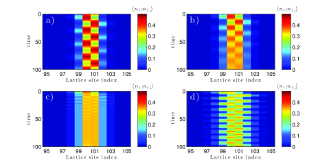
Figure 1: Time dependence of the local doublon density $\langle n_{i\,\uparrow}n_{i\,\downarrow}\rangle$ for $|U|/J=10$ and $N_{\uparrow}$= 20 (a), 60 (b), 140 (c), 180 (d). Horizontal axis: site index $i$, vertical axis: time (in units of $J^{-1}$). In the simulations we first calculate the ground state of the lattice (number of lattice sites $L=200$) loaded with one impurity ($N_{\downarrow}=1$), in presence of a bath of spin-up particles (different simulations were performed with varying numbers of up particles $N_{\uparrow}=[1,\,10,\,20\dots 180,\,190,\,200]$), whose description is provided by the Hubbard Hamiltonian. In addition to the attractive interaction between spin-up and spin-down particles, characterized by the parameter $U$, the impurity is confined by a parabolic potential of the form $Vi^{2}$, with $i$ the site index, and $V/J=0.1$. At $t=0^{+}$, the down particle is kicked with quasi-momentum $k=0.1\pi$. As is described in the text, it is possible to see that, as a function of $N_{\uparrow}$, the dynamics exhibits different regimes, characterized by a transition from doublon-oscillations to a regime where the internal dynamics of the polaron dominates, and eventually to free-particle oscillations. All simulations are performed with a TEBD code, with the following numerical parameters: lattice size $L=200$, unless otherwise stated; Schmidt number $\chi=80$; initial imaginary timestep (ground-state calculation) $\delta t_{i}=0.1J^{-1}$; timestep (real time evolution) $\delta t=0.02J^{-1}$ (throughout the paper $\hbar=1$, and the length scale is set equal to the lattice spacing $a$, see text). After testing with larger values of the Schmidt number, we have used the value $\chi=80$ which provides accurate results both for the ground state and the time evolution. The reason of the effectiveness of this rather small value of $\chi$ lies in the reduced size of the Hilbert space for a strongly imbalanced gas.

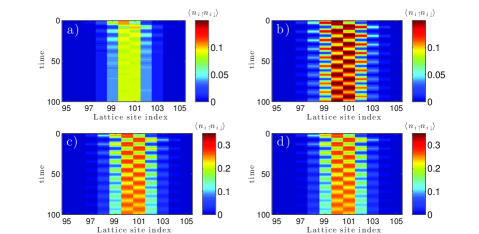
Figure 2: Time dependence of the local doublon density $\langle n_{i\,\uparrow}n_{i\,\downarrow}\rangle$ for $|U|/J=1$ and $N_{\uparrow}$= 20 (a), 60 (b), 140 (c), 180 (d). For $|U|/J=1$, the time evolution of $\langle n_{i\,\uparrow}n_{i\,\downarrow}\rangle$ is characterized by single-particle oscillations decreasingly damped for increasing bath particle population. For $N_{\uparrow}=20$, small-amplitude oscillations (not visible here, see Fig. 6) appear; these oscillations are associated with the pair-breaking mechanism as we will discuss in Sec. II.3. All simulation parameters (except $U$) are the same as in Fig. 1.

I.2 The non-interacting impurity

To provide a better description later on of the effects on the motion of the impurity that are induced by interactions with the bath, we first single out the dynamical effects induced by the concomitant presence of the harmonic trapping and the 1D lattice at $U=0$. That is, we consider a single particle in a potential formed by combining a lattice and a harmonic potential. As shown in Rey et al. (2005), if the particle is initially in the ground state of the combined potential, and then the harmonic trap is displaced by an amount $\delta$, the expectation value of the particle position is

$$\langle x\rangle=\delta\exp\left[-\left(\frac{\delta}{a_{\rm ho}}\right)^{2}\sin^{2}\left(V/8t\right)\right]\cos\left[V\left(\sqrt{\frac{2}{Vm_{\rm eff}}}-\frac{1}{4}\right)t-\frac{\delta^{2}}{2a_{\rm ho}^{2}}\sin\left(\frac{Vt}{4}\right)+\frac{\pi}{2}\right],$$ (2)

where $V$ is the strength of the trapping potential, and $m_{\rm eff}$ is the effective mass of the particle in the lattice, which for our choice of units ( $a=1$) is $m_{\rm eff}=0.5J^{-1}$. The harmonic oscillator length is defined via the trapping frequency $\omega$ and the mass of the particle as $a_{\rm ho}=1/\sqrt{m_{\rm eff}\omega}$, and on the other hand the strength of the harmonic oscillator potential $V=m_{\rm eff}\omega^{2}/2$: thus $a_{\rm ho}=(2m_{\rm eff}V)^{-1/4}$ and with $m_{\rm eff}=0.5J^{-1}$ we then should have $a_{\rm ho}=(V/J)^{-1/4}$.

Our initial conditions involving a finite quasi-momentum kick differ from those in Ref. Rey et al. (2005), where the harmonic trap is initially displaced by an amount $\delta$. To account for this difference, we need to introduce a $\pi/2$ phase in the cosine term of Eq. 2, and also compute the value of $\delta$ corresponding to our initial momentum kick. We can do this by matching the energy of the initial state in each case. The energy for the state at $t\to 0^{+}$ is given by the lowest eigenenergy of the combined harmonic trap and lattice system (Eq. (14) of Rey et al. (2005)), with the addition of the kinetic energy given by the kick of a quasi-momentum $k$. If, by a semiclassical argument, we assume that this energy must be converted to potential energy (removing the zero-point energy from both terms), then we have

$$V\left(\delta^{2}+\frac{1}{16}+\frac{\sqrt{V/J}}{256}\right)=(1-\cos k)/m_{\rm eff}.$$ (3)

The left hand side of Eq. (3) represents the small $V$ expansion of the potential energy of a particle in a 1D lattice in the presence of harmonic confinement when displaced by $\delta$ from the minimum of the potential, while the right hand side is its kinetic energy. We can thus deduce an approximate expression for $\delta$

$$\delta=\left[\frac{1-\cos k}{Vm_{\rm eff}}-\frac{1}{16}-\frac{\sqrt{V/J}}{256}\right]^{1/2}.$$ (4)

Combining Eqs. (2) and (4), we obtain the relation between the centre of mass oscillation frequency $\omega_{COM}$ and the theoretical value of the mass of the different particles

$$\omega_{COM}=V\left[\left(\sqrt{\frac{2}{m_{\rm eff}V}}-\frac{1}{4}\right)-\frac{\sqrt{V/J}}{4}\left(\frac{1-\cos k}{m_{\rm eff}V}-\frac{1}{16}-\frac{\sqrt{V/J}}{256}\right)\right].$$ (5)

As a benchmark, we have compared the frequency given by Eq. (5) with the value obtained from the numerical simulations for a free particle ($m_{\rm eff}=0.5$), and we have found good agreement between analytical and numerical values.

II Dynamics of an impurity in a fermionic bath

In the following, we characterize the different physical states which the impurity may form inside the bath. The key observable in our analysis is the oscillation of the time-dependent doublon density, defined as $\langle n_{i\,\uparrow}n_{i\,\downarrow}\rangle(t)$, after a kick with quasi-momentum $k=0.1\pi$ has been imparted to the impurity at $t=0^{+}$. We find that this is a more useful quantity than the impurity density $\langle n_{i\,\downarrow}\rangle(t)$, as it provides more direct information corresponding to the bath dynamics and pairing with the impurity.

Examples of the oscillatory motion of the doublon density are shown in Figs. 1 and 2 in the regime of strong ($|U|/J=10$) and weak ($|U|/J=1$) attraction respectively. In the strongly attractive case, we see the oscillation frequency shifting as a function of the bath filling, increasing only slightly while the bath density is below half filling, but jumping to much larger values above, from where it decreases again as the density approaches integer filling. Conversely, in the case of weak attraction the oscillation frequency only decreases slightly for low and high densities, and is roughly the same for all intermediate densities.

The observable that encapsulates all these behaviours is the doublon centre of mass ($\mathcal{X}_{\uparrow\,\downarrow}$), defined as

$$\mathcal{X}_{\uparrow\,\downarrow}(t)=\frac{\sum_{i}\left(i-\frac{L-1}{2}\right)\langle n_{i\,\uparrow}n_{i\,\downarrow}\rangle(t)}{\sum_{i}\langle n_{i\,\uparrow}n_{i\,\downarrow}\rangle(t)},$$

which is extracted from the full density and is shown in Figs. 3 and 4.

As is explained in detail in the following sections for the different interaction and bath density regimes, we gain insight into the physics of the system by analysing the Fourier transform of $\mathcal{X}_{\uparrow\,\downarrow}(t)$, $\mathcal{X}_{\uparrow\,\downarrow}(\omega)$, which is shown in Figs. 5 and 6 for strong and weak attraction. For strong attraction, $\mathcal{X}_{\uparrow\,\downarrow}(\omega)$ shows that the oscillation of a tightly bound on-site pair dominates the dynamics at low density, while a polaron-like state is present but weak (low- and high-frequency peaks in Fig. 5-a respectively). The relative weights of the polaronic and bound-pair peaks reverse as the density of bath atoms increases above $0.5$, with the polaron component becoming predominant and the bound-pair peak almost vanishing (high- and low-frequency peaks in Fig. 5-b respectively; notice e.g. how for $N_{\uparrow}=140$ the bound-pair peak has become essentially just a broad shoulder).

In order to understand the physics of the bound pair for strong interactions between impurity and bath atoms, we make use of the so-called string hypothesis from the Bethe-ansatz solution of the Hubbard model (c.f. Appendix V.1). Using this, we see that a tightly-bound on-site pair dominates at low bath fillings, and can be understood in a two-body picture, where we can compute formulas for the pair oscillation frequency, as shown in Fig. 7. On the other hand, the polaron-like state dominating at higher densities can be explained by the scattering of bath particles from the Fermi surface to the edge of the Brillouin zone meditated by the oscillating impurity . We find that the frequency of the resultant peak in $\mathcal{X}_{\uparrow\,\downarrow}(\omega)$ is insensitive to the value of both interaction strength $U$ and initial momentum kick $k$. We also examine the way the impurity modifies the density of the bath around its position and explain why the peak position stays independent of $U$ despite this local distortion. Subsection II.2 describes this in detail, including the change in the polaron oscillation frequency with density.

By contrast, in the case of weak interaction, a polaron component to the oscillation is significant only for densities at or below $0.2$ (low-frequency peak in Fig. 6-a), while the dominant component of $\mathcal{X}_{\uparrow\,\downarrow}(\omega)$ stems from the motion of a free particle (low- and high-frequency peaks in Figs. 6-a and b, respectively). In this regime the polaronic component corresponds to the resonant scattering between a bound pair and an impurity particle propagating through the background particle bath. This will be described in section II.3.

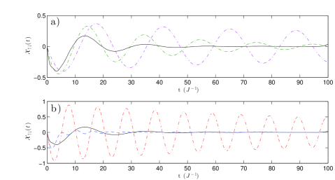
Figure 3: The doublon centre of mass $\mathcal{X}_{\uparrow\,\downarrow}(t)$ for $|U|/J=10$ and (a) $N_{\uparrow}=$ 20 (purple curve), 60 (green dash-dotted curve), 100 (black continuous curve); and (b) $N_{\uparrow}=$ 100 (black continuous curve), 140 (blue dashed curve), 160 (red curve). In panel (a), it is possible to see how the centre-of-mass oscillations associated with the doublon dynamics are increasingly damped when the bath population increases towards half filling. Above half filling, the oscillations associated to the polaron internal dynamics (described in Sec. II.2) start to appear, reaching the free-particle oscillation frequency for $N_{\uparrow}\to L$. The deviation of $\mathcal{X}_{\uparrow\downarrow}$ for $t\to 100J^{-1}$ is a finite-size effect. It corresponds to the time for which excitations in the bath are reflected back from the system boundaries to the centre of the trap, affecting thus the doublon dynamics. All simulation parameters are the same as Fig. 1.

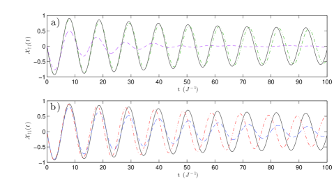
Figure 4: The centre of mass $\mathcal{X}_{\uparrow\,\downarrow}(t)$ for $|U|/J=1$ and (a) $N_{\uparrow}=$ 20 (purple dashed curve), 60 (green dash-dotted curve), 100 (black continuous curve), and (b) $N_{\uparrow}=$ 100 (black continuous curve), 140 (blue dashed curve), 160 (red curve). For $|U|/J=1$, the oscillations are dominated by the single-particle oscillation frequency $\omega/J\simeq 0.62$, and increasingly damped for decreasing bath population. All simulation parameters are the same as in Fig. 2.

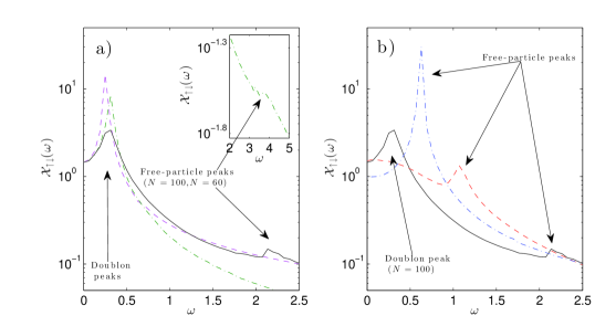
Figure 5: The doublon centre of mass $\mathcal{X}_{\uparrow\,\downarrow}(\omega)$, $|U|/J=10$. The Fourier analysis allows a quantitative estimation of the oscillation frequencies for different values of $N_{\uparrow}$, complementing the description given in Fig. 3. (a) $N_{\uparrow}=$ 20, 60, 100 (purple dashed, green dash-dotted and black continuous curves). For $N_{\uparrow}=$ 20 only the doublon peak for $\omega/J\simeq 0.5$ is present, while for $N_{\uparrow}=$ 100 the polaron internal dynamics peak appears, for $\omega/J\simeq 2.1$ respectively, and for $N_{\uparrow}=$ 60 the precursor of the polaron peak starts to appear around $\omega/J\simeq 3.8$. The inset shows additional data for higher values of $\omega$ . (b) $N_{\uparrow}=$ 100, 140, 180 (black continuous, blue dashed, and red dash-dotted curve). The polaron internal dynamics peak shifts to the left for increasing interaction ($\omega/J\simeq$ 2.1, 1.1, 0.8 for $N_{\uparrow}=$ 100, 140, 180), while the doublon peak is increasingly damped. All simulation parameters are the same as in Fig. 1.

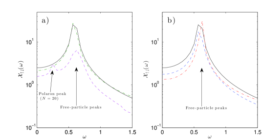
Figure 6: $\mathcal{X}_{\uparrow\,\downarrow}(\omega)$, $|U|/J=1$. (a) $N_{\uparrow}=$ 20, 60, 100 (purple dashed, green dash-dotted and black continuous curves) and (b) $N_{\uparrow}=$ 100, 140, 180 (black continuous, blue dashed, and red dash-dotted curve). For $N_{\uparrow}=$20 both the polaron and the free particle peaks are present ($\omega/J\simeq$ 0.4, 0.8 respectively, while for larger values of $N_{\uparrow}$, only the free particle peak is present. All simulation parameters are the same as Fig. 2.

II.1 Strong interactions: the low-frequency peak

In a 1D Hubbard model with strong interactions, Bethe-ansatz techniques provide two sets of solutions, which together cover all possible eigenstates of the system - provided we assume the so-called string hypothesis to be correct Essler et al. (2005). In each of these two sets of solutions, A and B, the total energy $E$ and quasi-momentum $P$ of a many-body state can be expressed in terms of Bethe-ansatz quantum numbers $\{k_{i}\}$ and $\Lambda$.

For the solutions of type A

$$P=\sum_{j=1}^{N}k_{j}\qquad E=-2J\sum_{j=1}^{N}\cos\left(k_{j}\right)+const.$$ (6)

and for the solutions of type B,

$$P=\sum_{j=1}^{N-1}k_{j}+2q\qquad E=-2J\sum_{j}^{N-1}\cos\left(k_{j}\right)-4J\cosh\xi\cos\left(q\right)+const.$$ (7)

where $\xi$ is defined by

$$\cosh\xi=\sqrt{1+\frac{U^{2}}{16J^{2}\cos^{2}\left(q\right)}}$$ (8)

and $q$ is the real part of the quantum numbers associated with the $k-\Lambda$ string (see Appendix V.1). In the strong coupling limit, it is possible to show that

$$-4J\cosh\xi\cos q\to U-4J^{2}/\left|U\right|-4J^{2}/\left|U\right|\cos\left(\kappa\right)+O\left(\frac{1}{U^{2}}\right),$$ (9)

where $\kappa=2q$ is the total quasi-momentum of the pair.

The eigenstates of type A correspond to the effectively free motion of both bath particles and the impurity, while solutions of type B correspond to a bound state of the impurity with one bath atom (with the remaining $N_{\uparrow}-1$ bath atoms again moving freely) (see Appendix V.1). For an attractive interaction, the B-type solutions are always energetically favorable, and for $|U|/J>2$ there is no overlap between the bands associated with type-A and type-B solutions.

Thus focussing on the B-type manifold of eigenstates, we can describe the observed behaviour of the low-frequency peak in $\mathcal{X}_{\uparrow\downarrow}(\omega)$ at large $|U|$ (c.f. Fig. 5) by deriving the explicit expression for the many-body energy $E$ in Eq. (7) as a function of the doublon quasi-momentum $\kappa$ (see Appendix V.1) to be

$$E_{\kappa}=-\sqrt{U^{2}+16J^{2}\cos^{2}\left(\kappa/2\right)},$$ (10)

where the dependency of the energy on the other $N_{\uparrow}-1$ quasi-momentum quantum numbers $\{k_{i}\}$ has not been taken into account, being irrelevant in the dynamics here considered. From this, the effective mass of the tightly bound pair can be extracted to be

$$m_{\rm doublon}=\left[\left(\frac{\partial^{2}E}{\partial\kappa^{2}}\right)\right]^{-1}_{\kappa\to 0}=\frac{1}{J}\sqrt{1+\frac{U^{2}}{16J^{2}}}\xrightarrow{|U|/J\gg 1}\frac{|U|}{4J^{2}},$$ (11)

which, in the limit $|U|/J\ll 1$, coincides with the expression that would be obtained from second-order perturbation theory.

It is interesting to note that our Bethe ansatz solution delivers the same result for the quasi-momentum dependence of the doublon contribution to the energy as the simple solution to the problem of two distinguishable bound particles on a lattice does Winkler et al. (2006); Valiente and Petrosyan (2008). In Fig. 7 we show the comparison between the numerical value of the doublon peak oscillation frequency (low-frequency peak in the strong-interaction regime), and the theoretical value obtained using our value for the doublon mass (11) in conjunction with Eq. (5). The excellent agreement shows that the doublon dynamics is well-captured by our Bethe-ansatz based model.

Figure 7: Comparison between the numerical value of the low-frequency peak oscillation frequency for the large interaction case (as extracted from $\mathcal{X}_{\uparrow\downarrow}(\omega)$), and the theoretical value for $|U|/J>1$, given by Eqs. (10) (11)). This comparison allows us to establish that the low-frequency oscillations of $\mathcal{X}_{\uparrow\,\downarrow}$ can be described in terms of oscillations of a particle (composed by one spin-up and one spin-down particle) in a parabolic confining potential. All simulation parameters are the same as in Fig. 1, except the interaction strength and the lattice size. Here $|U|/J=$3, 5, 10, 20 and $L=$ 200 or 400. The error bars account for the finite resolution of the Fourier transform. Larger lattices allow for longer simulation times before the reflection from the edges starts playing any role in the doublon dynamics, thus allowing higher resolutions in the frequency domain. It is worth noting that the full Bethe-ansatz formula works even for moderately weak interaction. The characteristic size of the composite particle is given by $\xi^{-1}$ (see Fig. 15), corresponding to a value of $\simeq 2.3$ for $|U|/J=3$.

II.2 Strong interactions: the high-frequency peak

In the case of strong attraction (large $|U|$) treated in this section, the oscillations of the doublon density also show another, high-frequency component in $\mathcal{X}_{\uparrow\downarrow}(t)$, which is weak for low bath densities, but which becomes significant above half-filling (see Fig. 5). Here, we argue that this feature can be understood in terms of an effective scattering of bath particles from the Fermi surface off the oscillating impurity towards the edge of the Brillouin zone. We will show that the position of this high-frequency peak in $\mathcal{X}_{\uparrow\,\downarrow}(\omega)$ depends primarily on the filling fraction in the bath, and the associated value of $k_{F}$, and is essentially independent of the kick strength and insensitive to $U$.

II.2.1 Description of the dynamics in terms of particle-hole excitations of the bath

The high-frequency peak in the strongly interacting limit can be understood in terms of scattering between two bath particles mediated by the presence of the impurity, together with the dynamics of the impurity itself. Within the framework of a two-band model (see Fig. 8), the effective scattering between bath particles is explained in terms of an exchange process, involving the transfer of the up particle from the tightly bound pair to the $\uparrow$-particle band above the Fermi level, and the concomitant transfer of a particle from the Fermi surface to the tightly bound pair (see Fig. 8).

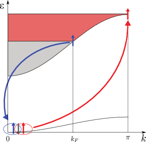
Figure 8: Two-band process leading to the scattering of a bath particle from $k_{F}$ to $\pi$. The specific pair-mediated process depicted here ($k_{P}=\pi$) represents the process associated with the maximum energy transfer from the pair to the bath. The promotion of an $\uparrow$ particle from the pair to the bath is allowed for $k_{F}<k<\pi$, while for $0<k<k_{F}$ the process is forbidden due to Pauli blocking.

The total energy necessary for this process, which the initial kick must supply now, involving both the scattering process as well as the impurity dynamics, is given by

$$\Delta E=\omega_{hi}+2J\left[(1-\cos k_{p})-(1-\cos k_{F\,\uparrow})\right],$$ (12)

where $\omega_{hi}$ is the oscillation energy associated with the dynamics of the impurity in a completely full bath-particle band. The frequency $\omega_{hi}$ thus corresponds to the oscillation frequency of a free particle in the lattice, in presence of the parabolic confining potential $V$, and its value can be calculated from Eq. (5).

The term $2J(1-\cos k_{p})$ corresponds to the transfer of an ”$\uparrow$” particle from the tightly bound pair to a free state of the bath above the Fermi level, as sketched in Fig. 8. The term $(1-\cos k_{F\,\uparrow})$ then is related to the transfer of an $\uparrow$-particle from the Fermi surface of the bath to the bound state of the $\uparrow\downarrow$- pair.

In Fig. 9, we show how the position of the high-frequency peak depends on the bath density - provided by numerics - and that it is in reasonable agreement with the expression given by Eq. (12) when $k_{p}=\pi$, corresponding to the largest possible energy associated with the transfer of an $\uparrow$-particle from the pair to the bath (see Fig. 8). We further find the peak position to be insensitive to changes in $U$ and kick strength $k$.

The offset between numerical results and eq. (12) is then related to the nonuniform spatial distribution of $k_{F}$ for the bath particles. This nonuniformity, in turn, is due to the perturbing effect of the impurity, which can be approximated as Friedel oscillations in the bath as we will show below. As the spatial extent of Friedel oscillations does not depend on $|U|$, the spatial distribution of $k_{F}$ and consequently $\Delta E$ are independent of the strength of the interaction. These findings go some way towards explaining why even the local density disturbance of the bath by the impurity is congruent with the observed $U$-independence of the high-frequency peak.

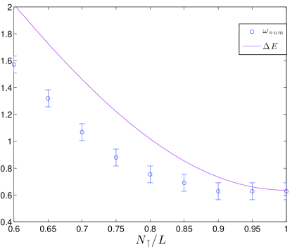
Figure 9: Plot of the high-frequency peak as a function of the bath filling, compared to the value of $\Delta E$ obtained from Eq. (12), for $k_{p}=\pi$. The position of the peaks in the numerical results does not show any dependence on $k$ and $U$: the value of $\omega_{num}$ coincides for $k=0.05\pi,\,0.1\pi,\,0.25\pi$ and $|U|=10$, and $k=0.1\pi$ and $|U|=5$.

II.2.2 Bath-particle distribution in presence of an impurity

With attractive interactions and an impurity that is localized by the tight parabolic confinement potential, the density of bath particles is modified locally in the center of the system. Let us denote the size of this modified region of the bath by $\zeta$. We make a first estimate for the value of $\xi$ by considering the limiting case $U\to-\infty$, with the impurity being located on a single site, $i$. In this case, due to the limit of infinite attraction, the site $i$ will act as a hard-wall boundary condition Matveev et al. (1993); Fabrizio and Gogolin (1995), and the density profile of the bath particles around the impurity will undergo Friedel oscillations Friedel (1958) (see Fig. 10), as was recently pointed out in Lamacraft (2009) for repulsive interaction and in absence of the lattice, according to the following formula

$$\rho_{\uparrow}(j)=\frac{N_{\uparrow}}{L}-\frac{1}{2\pi}\frac{\sin\left[2k_{F\,\uparrow}\left(j-i\right)\right]}{|j-i|}.$$ (13)

We note that in a 1D system the period of these oscillations is always independent of the strength of the interactions between the bath particles and the bath impurity interactions, and is always $(2k_{F\,\uparrow})^{-1}$ for a fermionic bath, and $(2\pi\rho_{0})^{-1}$ for a bosonic one - all that changes with the interaction is the amplitude of the Friedel oscillations.

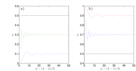
Figure 10: Friedel oscillations (see Eq. (13)) induced by the presence of a hard-wall boundary condition at $j=(L-1)/2$ for (a) 20 (purple dashed curve), 60 (green dash-dotted curve), 100 (black continuous curve), and (b) 100 (black continuous curve), 140 (blue dashed curve), 180 (red dash-dotted curve) bath particles respectively (see Eq. (13)).

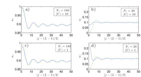
Figure 11: Comparison between the numerical estimate of the ground-state spatial oscillations induced in the bath by (a,c,d) a single down impurity or (b) a doublon (blue continuous curves), with the Friedel oscillations induced by hard-wall boundary conditions (green dash-dotted curves), with (a) $N_{\uparrow}=180$, $|U|/J=10$, (b) $N_{\uparrow}=20$, $|U|/J=10$, (c) $N_{\uparrow}=180$, $|U|/J=1$, (d) $N_{\uparrow}=20$, $|U|/J=1$. In the high-density limit, the agreement between the numerical calculations and the approximate model is good, while, in the low-density limit, the numerical results suggest that the role of the impurity cannot be described in terms of an impurity-induced Hartree potential. This hypothesis is confirmed by the exact diagonalisation of an Hamiltonian describing a spin-polarized gas in presence of a localized potential mimicking the potential induced by the impurity. In this case the results are compatible with the results implied by Eq. (13). All simulation parameters are the same as in Fig. 1 and Fig. 2.

In Fig. 11, we show how approximating either the on-site bound pair (in case of strong attraction) or the single particle (for weak attraction) as a boundary condition located at the minimum of the parabolic potential works well to describe the density modulation induced in the bath when $N_{\uparrow}$ is large, while it fails in the case of a more dilute system. As we have been focussing on just this regime of intermediate and high filling in this part, this approximation should be very reasonable.

II.3 Weak interactions

As anticipated, for interactions $|U|\leq 1$, the peak in $\mathcal{X}_{\uparrow\,\downarrow}(\omega)$ associated with the oscillation of a tightly bound on-site pair is not present. Nevertheless, we observe two distinct modes in the doublon-density center-of-mass oscillations $\mathcal{X}_{\uparrow\,\downarrow}(t)$ in the weakly interacting regime as well. One of them appears due to the free oscillatory motion of a non-interacting particle as derived in Sec. I.2. Another peak, at lower frequencies, appears as well (see Figs. 6 and 12).

The underlying physics of this low-frequency peak derives from a resonant transition between a bound pair and scattering states, specifically the spin-down impurity at zero quasi-momentum and a spin-up bath particle at the Fermi quasi-momentum $k_{F\uparrow}$. The frequency of this peak can thus be obtained considering the difference between the energy of the (weakly-bound) pair and the energy of the scattering state

$$\omega_{pol}=E_{\uparrow}+E_{\downarrow}-E_{\uparrow\,\downarrow}=-2J\left[1+\cos(k_{F\,\uparrow})\right]+\sqrt{U^{2}+16J^{2}}.$$ (14)

Figure 12 shows the excellent agreement between this model and the numerical results from the TEBD calculations, within the error bars set by the finite resolution of the Fourier transform.

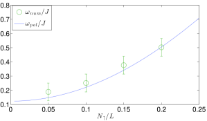
Figure 12: Comparison between the numerical value of the low-frequency peak at $|U|/J=1$ and $\omega_{pol}$ corresponding to the resonant frequency of the bound-doublon to scattering-states transition. This peak can be seen in the $N_{\uparrow}=20$ plot (small peak around $\omega\simeq 0.2$ in Fig. 6). Above $N_{\uparrow}/L\simeq 0.2$ it merges with the free-particle peak, and eventually disappears. In this picture, the spin-up bath particles are resonantly bound to the spin-down impurity, analogous to the case of static polarons. All simulations parameters are like in Fig. 2. The errorbars account for the finite resolution of the Fourier transform.

Further, the existence of the two peaks in $\mathcal{X}_{\uparrow\,\downarrow}(\omega)$ can be related to the known structure of the polaron ground state: in the the polaron ansatz Chevy (2006) of the type

$$|\Psi\rangle=\sqrt{Z}c^{\dagger}_{0\downarrow}|FS\rangle_{\uparrow}|0\rangle_{\downarrow}+\sum_{k>k_{F}^{\uparrow},q<k_{F}^{\uparrow}}\phi_{k,q}c^{\dagger}_{k\uparrow}c_{q\uparrow}c^{\dagger}_{q-k\downarrow}|FS\rangle_{\uparrow}|0\rangle_{\downarrow},$$ (15)

the first term describes the impurity at rest in the presence of the unperturbed Fermi sea of the bath (with the quasiparticle weight $Z$), and the second term a coherent superposition of states, in which the motion of the impurity is correlated with a single particle-hole excitation of the Fermi sea (like the weakly bound state entering Eq. (14)).

We can hypothesize that the high-frequency “free particle” peak in $\mathcal{X}_{\uparrow\,\downarrow}(\omega)$ corresponds to a second-order process involving the virtual breaking of a pair, while the low-frequency peak is caused by breaking up the correlated state between impurity and a particle-hole excitation of the Fermi sea.

$t=0^{+}$, both parts of Eq. (15) dynamics. Based on our results, we can hypothesize that the first term of Eq. (15) leads to peak in $\mathcal{X}_{\uparrow\,\downarrow}(\omega)$, while the second term causes the correlated state between impurity and a particle-hole of the Fermi-sea, as we have shown through the agreement of Eq. (14) with our simulation data 12). The relative height of the peaks could perhaps provide a useful tool for determining the two terms in Eq. (15).

II.4 Damping

Along the lines of the above discussion about the particle-hole excitation process, it is possible to intuitively understand the oscillation damping. When approaching half-filling, both from the low- and the high-density limit, the oscillation damping is increased. This increase is associated with the increase of the particle-hole creation mechanism through the virtual breaking of a pair for increasing filling, and the concomitant energy transfer increase for decreasing filling. This mechanism of dissipation is confirmed by the observation in the numerical data of density perturbations in the bath particles, propagating at $2J$, consistent with the picture of the transfer of bath particles to the top of the band $k=\pi$.

III The kicked impurity in a bosonic reservoir

Comparing the results obtained for a fermionic reservoir to those from a bosonic one enables us to state which features of the observed dynamics are universal, and which are particular to the fermionic bath. Towards this, we have performed TEBD simulations for a two-species Bose-Hubbard Hamiltonian

$$H=-J\sum_{i\,\sigma}b_{i\sigma}^{\dagger}b_{i+1\sigma}+h.c.+U\sum_{i}n_{i\,\uparrow}n_{i\,\downarrow}+\frac{W}{2}\sum_{i}n_{i\,\uparrow}(n_{i\,\uparrow}-1)+V\sum_{i}n_{i\,\downarrow}\left(i-\frac{L-1}{2}\right)^{2},$$ (16)

where trap parameter $V$, tunneling $J$ and the values of $U$ and $N_{\uparrow}$ are the same as described in section I, as is the impurity preparation and the initial kick to the impurity (as in the fermionic case we will set $J=1$, $a=1$). The two key differences are that now $b_{i\,\sigma}$, $b_{i\,\sigma}^{\dagger}$ are operators for softcore bosons, which interact repulsively on-site with energy $W$, if $\sigma=\uparrow$. Here, we have considered $W/J=4,10,20$.

III.1 The weak interaction limit

Repeating the TEBD simulations for weak interactions between the impurity and a bosonic bath, we find that the two-peak structure discussed in II.3 persists for all values of $W$ we have simulated, as shown in Fig. 13. Moreover, the position of the polaron-dissociation peak (c.f. II.3) is still described remarkably well by the theory for the fermionic bath, even for the lowest value of $W$, $W/J=4$. These findings can be understood analytically by observing that, at low densities and reasonably large values of $W$, one-dimensional lattice bosons map to spinless fermions with weak nearest neighbor attractions. This mapping is achieved by describing the sector of low-energy, long-wavelength excitations of the $\uparrow$ component of the Hamiltonian (16) as a Tomonaga-Luttinger liquid (TLL), whose properties are characterized by the so-called TLL parameters, $K_{b}$ and $v_{b}$ Cazallila et al. (2011). Expanding the $\uparrow$-sector in Hamiltonian (16) and the bath density operator $n_{x\,\uparrow}$ in terms of the canonically conjugate TLL field operators $\phi_{\uparrow}(x)$ and $\theta_{\uparrow}(x)$, one obtains

$$H \approx \frac{1}{2\pi}\int dx\left(u_{b}K_{b}(\partial_{x}\theta_{\uparrow}(x))^{2}+\frac{u_{b}}{K_{b}}(\partial_{x}\phi_{\uparrow}(x))^{2}\right)+U\sum_{i}\left(\rho_{0}-\frac{\partial_{x}\phi_{\uparrow}(x_{i})}{\pi}\right)\left(\sum_{m=-\infty}^{\infty}e^{2im[\pi\rho_{0}x_{i}-\phi_{\uparrow}(x)]}\right)n_{i\,\downarrow}$$ (17)

$$+J\sum_{i}b_{i\downarrow}^{\dagger}b_{i+1\downarrow}+h.c.+V\sum_{i}n_{i\,\downarrow}\left(i-\frac{L-1}{2}\right)^{2},$$

where expanding the impurity-bath coupling in this way presupposes that the impurity does not distort the bath density too much locally. In the limit of large $W/J$, the TLL parameters are known perturbatively, $K_{b}\approx 1+\frac{4J}{\pi W}\sin\pi\rho_{0}$, $u_{b}=2J\sin\pi\rho_{0}\left(1-\frac{4J}{W}\rho_{0}\cos\pi\rho_{0}\right)$

Now, a bath of spinless lattice fermions with attractive nearest-neighbor interactions $V_{nn}$ and Fermi quasi-momentum $k_{F}$ coupled to an impurity with an on-site density-density interaction, can be mapped to a TLL in 1D in a manner identical to (17), where $K_{b}$ is replaced by $K_{f}$ and $u_{b}$ by $u_{f}$ Giamarchi (2003). These parameters are also known from perturbation theory for small $V_{nn}$: $K_{f}=1+\frac{V_{nn}(1-\cos 2k_{F})}{2\pi\sin k_{F}}$, $u_{f}=2J\sin k_{F}\left(1-\frac{V_{nn}(1-\cos 2k_{F})}{2\pi J\sin k_{F}}\right)$.

Computing $K_{b}$ and $u_{b}$ for densities between $0$ and $0.2$ and large $W/J$ shows that Eq. (17 ) can be read equivalently as the model of an impurity coupled to weakly nearest-neighbour attractive spinless fermions. For example, for $W/J=10$ and $n_{\uparrow}=0.1$, $K_{b}=1.039$, $u_{b}/J=0.59$, values that are best matched by $K_{f}$ and $u_{f}$ for $|V|/J=0.75$, $k_{F}=0.1\pi$. Crucially, a value of $K_{f}=1.039$ is still very close to the values for free fermions, $K_{f}=1$. Thus, the continued applicability of Eq. (14) - which had initially been developed from a one-body picture of the free fermion bath - to predict the polaron peak in the weak-coupling regime even for a (sufficiently repulsive) bosonic bath, can be explained (c.f. Fig. 13).

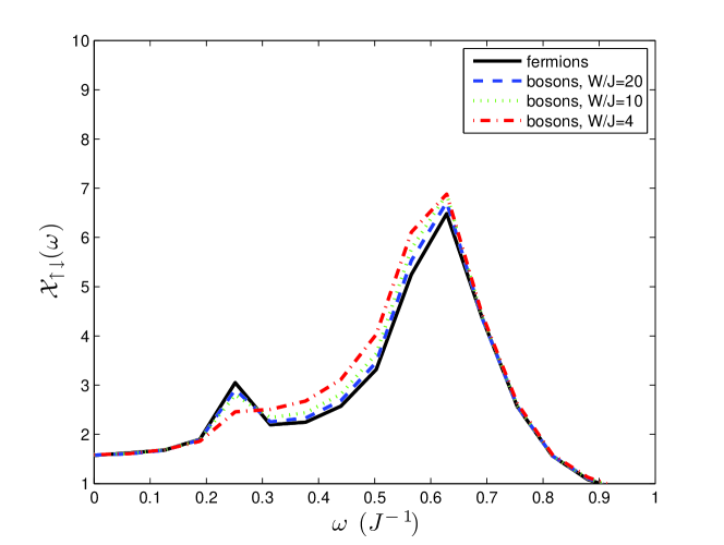
Figure 13: Comparison of $\mathcal{X}_{\uparrow\,\downarrow}(\omega)$ between fermions and bosons in the weak-attraction case, $|U|/J=1$, $N_{\uparrow}=20$. The position of the low-frequency peak for the fermionic bath, which stems from the break-up of correlated states between the impurity and particle-hole excitations in the bath (c.f. II.3), is very similar for the bosonic bath, at all values of $W$. See text for details.

III.2 The strong interaction limit - higher-order bound states of the impurity.

In the opposite limit of large bath-impurity attraction, $|U|\gg J$, the kick-induced dynamics of the impurity start to depend crucially on the ratio $|U|/W$. As an example, as for the fermions, we focussed on the case $|U|/J=10$. As long as $W>|U|$, the spectrum of doublon dynamics, $\mathcal{X}_{\uparrow\downarrow}(\omega)$, remains qualitatively unaltered from the case of the fermionic bath: when $n_{\uparrow}<0.5$, the dynamics of the kicked impurity are dominated by the oscillation of the doublon-mode, whereas for $n_{\uparrow}\geq 0.5$ this doublon peak increasingly flattens out and eventually disappears as $n_{\uparrow}$ increases above half-filling, as shown in Fig. 14. At the same time, like for fermions, a high-frequency peak appears for $n_{\uparrow}\geq 0.5$, increasing in amplitude as $n_{\uparrow}$ grows above the threshold while the doublon peak decreases, signaling the transition of the dynamics to a regime dominated by the virtual breaking of the pair (c.f. II.2). Even for a substantial value of $W$, $W/J=20$, the value of the oscillation frequency is higher than in the fermionic case, signalling an incomplete transition to a Tonks regime for the bosonic system.

for a range of densities, as frequency over the fermionic comparable to the size of the $n_{\uparrow}\approx 0.9$.

On the other hand, when the boson-boson repulsion $W$ becomes comparable to or smaller than the magnitude of the boson-impurity attraction $|U|$, the numerics clearly show that higher-order bound states between impurity and bath particles are formed in the ground state. At $W/J=|U|/J=10$, both doublon and trion states (the impurity binding to one or two bath particles on-site respectively) are present, whereas, for $W/J=4$ doublon, trion and quatrion bound states are occupied, with the trion state carrying the largest weight at any bath density. When quasi-momentum is applied to the impurity by the kick, these higher order bound states perform oscillations, at frequencies significantly lower than those for the doublons due to the even higher effective mass. Interestingly, the damping we observe becomes gradually smaller the smaller $W/J$ is, with the oscillations at $W/J=4$ showing almost no decay at any value of $n_{\uparrow}$ in the time domain over which we simulate. Whether this effect is due to the partial ability of 1D superfluids to be protected against excitations Kane and Fisher (1992); Giamarchi (2003) – which would be the source of any damping of the bound state oscillations - is an interesting question for further study.

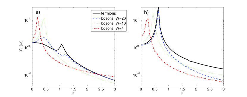
Figure 14: Comparison of $\mathcal{X}_{\uparrow\,\downarrow}(\omega)$ between fermions and bosons in the strong-attraction case, $|U|/J=10$. a) $N_{\uparrow}=140$. For the fermion bath (black solid line), the virtual pair-breaking peak (c.f. II.2) has become dominant, with the doublon peak at lower frequency having almost completely flattened out. For bosons at $W/J=20$ (blue dashed line), the behaviour is qualitatively similar, but the oscillation of the doublon is still dominant, as evidenced by the larger low-frequency peak. For $W/J=10$ (green dotted line) and $W/J=4$ (red dash-dotted line), only the high-order bound states oscillate, there is no virtual pair-breaking peak. b) $N_{\uparrow}=180$. For the fermion bath, the virtual pair-breaking peak (c.f. II.2) is now fully dominant, with the doublon peak at lower frequency having completely vanished. The dynamics for the boson bath at $W/J=20$ (blue dashed line), now almost completely matches that of the fermions, showing that for bosons as well virtual pair-breaking peak, corresponding to the fermionization of the bosonic gas. For $W/J=10$ and $W/J=4$, only the high-order bound states oscillate as in a), there is again no virtual pair-breaking peak.

IV Discussion and conclusions

The dynamics of the impurity moving on a 1D lattice inside a fermionic bath, or a strongly repulsive bosonic one, shows intriguingly complex dynamics, as can be seen by studying the time-evolution of the doublon density. One of the characteristic frequencies that appears corresponds to the motion of a free particle, appearing in the limit of high filling of the bath and is easily understood due to the increasingly uniform interaction energy the impurity experiences on all sites. Another feature of the dynamics, namely the oscillations of a bound pair are also rather intuitive to understand, allowing to draw an analogy to the molecule vs. polaron question in three dimensional continuum systems. The bound pair is present in regime of large $|U|/J$ and low density, like the molecule in the polaron vs. molecule analogy. In the limit of small $|U|/J$ , we observed the dynamics of a free particle side-by-side pair breaking of the correlated states of a polaron. This actually corresponds well to the polaron ansatz Chevy (2006) which is a superposition of a non-interacting Fermi sea (free particle) plus a contribution from correlated particle - hole states. Thus, the crossover from a polaron to a bound pair with increasing interaction is also taking place in analogy to higher dimensional continuum systems. In our system, however, we have a feature that does not have any analogy in the polaron vs.molecule crossover in 3D continuum, namely, the high-frequency peak in the large $|U|=J$ regime, which becomes dominant for bath fillings above 0.5, which is the result of a virtual particle-hole creation process. This virtual exchange of paired and bath particles can be read as a kind of internal dynamics of the polaron. Observation of the dynamics predicted here should be feasible in currently available ultracold gases systems, provided that the temperature is below the energy scale of the oscillations which we found to be of the order of $0.1J$-$1J$.

$|U|$ range	Bath population	Dynamics regime
Strong interaction	Large $N_{\uparrow}$	Free particle
Strong interaction	Intermediate $N_{\uparrow}$	Bound pair + polaron internal dynamics
Strong interaction	Small $N_{\uparrow}$	Bound pair
Weak interaction	Large $N_{\uparrow}$	Free particle
Weak interaction	Intermediate & small $N_{\uparrow}$	Free particle + polaron

Table 1: Table summarising the different regimes identified for the problem considered here.

Acknowledgements We thank J. Kajala for useful discussions. This work was supported by the Academy of Finland through its Centres of Excellence Programme (projects No. 251748, No. 263347, No. 135000 and No. 141039), by ERC (Grant No. 240362-Heattronics) and by the Swiss NSF under MaNEP and Division II. Work in Pittsburgh is supported by NSF Grant PHY-1148957. Computing resources were provided by CSC, the Finnish IT Centre for Science.

V Appendix

V.1 Effective mass from the Bethe ansatz

We show here how to gain some insight into the problem through the string hypothesis for the solution of the Lieb-Wu equations, whose solutions describe (most of) the eigenvalues of the Hubbard Hamiltonian in one dimension (Chapter 4 of Essler et al. (2005)), in the limit of large lattice lengths $L$. For a fixed total number of particles $N$ and number of down particles $M$, the patterns of which the solutions of the Lieb-Wu equations are composed can be classified in three different categories:

• $k-\Lambda$ strings;

• single real values of $k_{j}$;

• $\Lambda$ strings.

Every eigenstate of the Hubbard Hamiltonian can be represented in terms of a particular configuration of strings, containing $M_{n}$ $\Lambda$-strings, $M_{n}^{\prime}$ $k-\Lambda$ strings of length $n$ (in our case $n=1$), and $\mathcal{M}_{e}$ single $k_{j}$. Here $M_{n}$, $M_{n}^{\prime}$, $\mathcal{M}_{e}$ are related to the $N$ and $M$ by

$$M=\sum_{n=1}^{\infty}n\left(M_{n}+M_{n}^{\prime}\right)$$ (18)

$$N=\mathcal{M}_{e}+\sum_{n=1}^{\infty}2nM_{n}^{\prime}.$$ (19)

In our case $M=1$ implies the existence of two classes of string solutions

• $M_{n}=1$, $M_{n}^{\prime}=0$, $\mathcal{M}_{e}=L$: this solution is characterised by one $\Lambda$ string constituted by a single real value, $N$ real $k_{j}$s and no $k-\Lambda$ strings.

• $M_{n}=0$, $M_{n}^{\prime}=1$, $\mathcal{M}_{e}=L-2$: in this case the solution is characterised by $N-2$ real $k_{j}$s and one $k-\Lambda$ string, characterised by two (complex-valued) $k_{1,2}$s and one real $\Lambda$, related by

  $$\sin(k_{1,2})=\Lambda\pm iU/4J.$$ (20)

In terms of the string parameters, energy and quasi-momentum are given by

$$P =\left[\sum_{j=1}^{N-2M^{\prime}}k_{j}-\sum_{n=1}^{\infty}\sum_{\alpha=1}^{M_{n}^{\prime}}\left(2\operatorname{Re}\arcsin\left({{\Lambda^{\prime}}_{\alpha}}^{n}+niU/4J\right)-(n+1)\pi\right)\right]\mod 2\pi$$ (21)

$$E =-2J\sum_{j=1}^{N-2M^{\prime}}\cos\left(k_{j}\right)+4J\sum_{n=1}^{\infty}\sum_{\alpha=1}^{M^{\prime}_{n}}\operatorname{Re}\sqrt{1-\left({{\Lambda^{\prime}}_{\alpha}}+niU/4J\right)^{2}}.$$ (22)

For the two classes of solutions previously identified, see A and B above, take the following form

• $$P =\sum_{j=1}^{N}k_{j}$$ (23)

  $$E =-2J\sum_{j=1}^{N}\cos\left(k_{j}\right)+const.$$ (24)

• $$P =\sum_{j=1}^{N-1}k_{j}-2\operatorname{Re}\left[\arcsin\left(\Lambda+iU/4J\right)\right]$$ (25)

  $$E =-2J\sum_{j}^{N-1}\cos\left(k_{j}\right)+4J\operatorname{Re}\sqrt{1-\left(\Lambda+iU/4J\right)^{2}}+const.$$ (26)

The solution containing the $k-\Lambda$ string can be written in a more transparent form as

$$P =\sum_{j=1}^{N-1}k_{j}+2q$$ (27)

$$E =-2J\sum_{j}^{N-1}\cos\left(k_{j}\right)-4J\cosh\xi\cos\left(q\right)+const.$$ (28)

where $q=\operatorname{Re}\left[k_{1}\right]=\operatorname{Re}\left[k_{2}\right]$ and $\xi=\operatorname{Im}\left[k_{1}\right]=-\operatorname{Im}\left[k_{2}\right]$, with $k_{1}$ and $k_{2}$ belonging to the $k-\Lambda$ string. For the $k-\Lambda$ string it is possible to prove (see Essler et al. (2005) p. 134) that

$$\cosh\xi=\sqrt{1+\frac{U^{2}}{16J^{2}\cos^{2}\left(q\right)}}.$$ (29)

From the form of the wavefunction associated with the $k-\Lambda$ string, $\xi$ describes the (exponential) spatial decay of the pair, and thus $\xi^{-1}$ can be interpreted as the size of the pair.

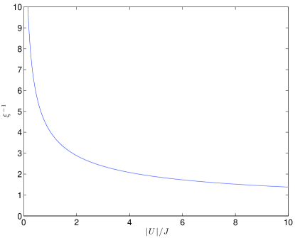
Figure 15: Pair size ($\xi^{-1}$) as a function of $U$.

In the strongly interacting limit we have

$$-4J\cosh\xi\cos q\to U-4J^{2}/\left|U\right|-4J^{2}/\left|U\right|\cos\left(2q\right)+O\left(\frac{1}{U^{2}}\right)$$ (30)

which is coherent with the strong coupling calculation leading to the Heisenberg Hamiltonian for the Hubbard Hamiltonian in the strong coupling limit (modulo a $U\to-U$ mapping).

The spectrum is thus constituted by a lower band ($k-\Lambda$+ single $k$s solutions) and a higher band (single $k$s and single $\Lambda$ solutions). Intuitively, the former correspond to a pair in an unpaired background Fermi sea, while the latter to scattering states. The down particle which is kicked in our simulations, with a view to the collective nature of the excitations in 1D systems, can be considered as constituted by both kinds of elementary excitations, appropriately weighted by the presence of the trapping potential.

We now aim at describing the dynamics that we observe numerically through the evaluation of the effective mass for the pairs

$$m_{\rm doublon} =\left.\left(\frac{\partial^{2}E}{\partial\kappa^{2}}\right)^{-1}\right|_{\kappa=0}$$ (31)

$$=\frac{1}{J}\sqrt{1+\frac{U^{2}}{16J^{2}}},$$ (32)

where $E$ is defined by Eq. (27).

V.2 The frequency of the non-interacting particle in the combined harmonic trap and lattice potential

The idea is to compare the oscillation frequency from the numerical data to the one given by the non-interacting particle in a combined lattice and harmonic trap potential. As a reminder, the formula for the centre of mass (COM) position was given by

$$\langle x\rangle=\delta\exp\left[\left(\frac{\delta}{a_{\rm ho}}\right)^{2}\sin^{2}\left(V/8t\right)\right]\cos\left[V\left(\sqrt{\frac{2}{Vm_{\rm eff}}}-\frac{1}{4}\right)t-\frac{\delta^{2}}{2a_{\rm ho}^{2}}\sin\left(\frac{Vt}{4}\right)+\frac{\pi}{2}\right].$$ (33)

Neglecting the exponential prefactor time dependence, we can write the centre-of-mass oscillation frequency as

$$\omega_{COM}=\frac{d\Omega}{dt},$$ (34)

where

$$\Omega=V\left(\sqrt{\frac{2}{Vm_{\rm eff}}}-\frac{1}{4}\right)t-\left(\frac{\delta}{a_{\rm ho}}\right)^{2}\sin\left(\frac{Vt}{4}\right)+\frac{\pi}{2}$$

with $\delta=\left[\frac{\left(1-\cos k\right)}{Vm_{\rm eff}}-\frac{1}{16}-\frac{\sqrt{V/J}}{256}\right]^{1/2}$, leading to

$$\omega_{COM}=V\left[\left(\sqrt{\frac{2}{m_{\rm eff}V}}-\frac{1}{4}\right)-\frac{\sqrt{V/J}}{4}\left(\frac{1-\cos k}{m_{\rm eff}V}-\frac{1}{16}-\frac{\sqrt{V/J}}{256}\right)\right].$$ (35)

The comparison between $\omega_{COM}$ and the numerical data is obtained by performing a discrete Fourier transform of $\langle n_{\uparrow}n_{\downarrow}\rangle(t)$ for different values of $U$ and $N_{\uparrow}$. For $N_{\uparrow}=N_{\downarrow}=1$, i.e. no bath, the agreement is perfect: higher interaction energies correspond to lower values of the oscillation frequency, in agreement with the increase of the effective mass.

References

- Mahan (2010) G. D. Mahan, Many Particle Physics (Springer, 2010), softcover reprint of hardcover 3rd ed. 2000 ed.
- Kondo (1964) J. Kondo, Prog. Theor. Phys. 32, 37 (1964).
- Lee and Wen (2006) P. A. Lee and X.-G. Wen, Rev. Mod. Phys. 78, 17 (2006).
- Ketterle et al. (1998) W. Ketterle, S. Inouye, M. R. Andrews, J. Stenger, H. J. Miesner, and D. M. Stamper-Kurn, Nature 392, 151 (1998).
- Bloch et al. (2008) I. Bloch, J. Dalibard, and W. Zwerger, Rev. Mod. Phys. 80, 885 (2008).
- Schirotzek et al. (2009) A. Schirotzek, C.-H. Wu, A. Sommer, and M. W. Zwierlein, Phys. Rev. Lett. 102, 230402 (2009).
- Nascimbène et al. (2009) S. Nascimbène, N. Navon, K. J. Jiang, L. Tarruell, M. Teichmann, J. McKeever, F. Chevy, and C. Salomon, Phys. Rev. Lett. 103, 170402 (2009).
- Sommer et al. (2011) A. Sommer, M. Ku, and M. W. Zwierlein, New J Phys 13, 055009 (2011).
- Koschorreck et al. (2012) M. Koschorreck, D. Pertot, E. Vogt, B. Fröhlich, M. Feld, and M. Köhl, Nature 485, 619 (2012).
- Kohstall et al. (2012) C. Kohstall, M. Zaccanti, M. Jag, A. Trenkwalder, P. Massignan, G. M. Bruun, F. Schreck, and R. Grimm, Nature 485, 615 (2012).
- Zhang et al. (2012) Y. Zhang, W. Ong, I. Arakelyan, and J. Thomas, Phys. Rev. Lett. 108, 235302 (2012).
- Chevy (2006) F. Chevy, Phys. Rev. A 74, 063628 (2006).
- Prokofév and Svistunov (2008) N. Prokofév and B. Svistunov, Phys. Rev. B 77, 125101 (2008).
- Massignan et al. (2008) P. Massignan, G. Bruun, and H. Stoof, Phys. Rev. A 78, 031602 (2008).
- Punk et al. (2009) M. Punk, P. Dumitrescu, and W. Zwerger, Phys. Rev. A 80, 053605 (2009).
- Zöllner et al. (2011) S. Zöllner, G. Bruun, and C. Pethick, Phys. Rev. A 83, 021603 (2011).
- Parish (2011) M. Parish, Phys. Rev. A 83, 051603 (2011).
- Massignan and Bruun (2011) P. Massignan and G. M. Bruun, Eur. Phys. J. D 65, 83 (2011).
- Giraud and Combescot (2012) S. Giraud and R. Combescot, Phys. Rev. A 85, 013605 (2012).
- Schmidt et al. (2012) R. Schmidt, T. Enss, V. Pietilä, and E. Demler, Phys. Rev. A 85, 021602 (2012).
- Baarsma et al. (2012) J. Baarsma, J. Armaitis, R. Duine, and H. T. Stoof, Phys. Rev. A 85, 033631 (2012).
- Ngampruetikorn et al. (2012) V. Ngampruetikorn, J. Levinsen, and M. M. Parish, Europhys. Lett. 98, 30005 (2012).
- Knap et al. (2012) M. Knap, A. Shashi, Y. Nishida, A. Imambekov, D. A. Abanin, and E. Demler, arXiv:1206.4962 (2012).
- Zvonarev et al. (2007) M. B. Zvonarev, V. V. Cheianov, and T. Giamarchi, Phys. Rev. Lett. 99, 240404 (2007).
- Zvonarev et al. (2009a) M. B. Zvonarev, V. V. Cheianov, and T. Giamarchi, Phys. Rev. Lett. 103, 110401 (2009a).
- Zvonarev et al. (2009b) M. B. Zvonarev, V. V. Cheianov, and T. Giamarchi, Phys. Rev. B 80, 201102(R) (2009b).
- Imambekov and Glazman (2008) A. Imambekov and L. I. Glazman, Phys. Rev. Lett. 100, 206805 (2008).
- Lamacraft (2009) A. Lamacraft, Phys. Rev. B 79, 241105 (2009).
- Giamarchi (2003) T. Giamarchi, Quantum Physics in One Dimension (Clarendon Press, Oxford, 2003).
- Essler et al. (2005) F. H. L. Essler, H. Frahm, F. Göhmann, A. Klümper, and V. E. Korepin, The One-Dimensional Hubbard Model (Cambridge University Press, 2005).
- Leskinen et al. (2010) M. Leskinen, O. Nummi, F. Massel, and P. Törmä, New J Phys 12, 073044 (2010).
- Guan (2012) X. W. Guan, Frontiers of Physics 7, 8 (2012).
- Mathy et al. (2012) C. J. M. Mathy, M. B. Zvonarev, and E. Demler, arXiv:1203.4819 (2012).
- Schecter et al. (2012) M. Schecter, A. Kamenev, D. Gangardt, and A. Lamacraft, Phys. Rev. Lett. 108, 207001 (2012).
- Palzer et al. (2009) S. Palzer, C. Zipkes, C. Sias, and M. Köhl, Phys. Rev. Lett. 103, 150601 (2009).
- Catani et al. (2012) J. Catani, G. Lamporesi, D. Naik, M. Gring, M. Inguscio, F. Minardi, A. Kantian, and T. Giamarchi, Phys. Rev. A 85, 023623 (2012).
- Peotta et al. (2012) S. Peotta, D. Rossini, M. Polini, F. Minardi, and R. Fazio, arXiv:1206.3984 (2012).
- Bonart and Cugliandolo (2012) J. Bonart and L. F. Cugliandolo, Phys. Rev. A 86, 023636 (2012).
- Bakr et al. (2010) W. S. Bakr, A. Peng, M. E. Tai, R. Ma, J. Simon, J. I. Gillen, S. Folling, L. Pollet, and M. Greiner, Science 329, 547 (2010).
- Sherson et al. (2010) J. F. Sherson, C. Weitenberg, M. Endres, M. Cheneau, I. Bloch, and S. Kuhr, Nature 467, 68 (2010).
- Fukuhara et al. (2012) T. Fukuhara, A. Kantian, M. Endres, M. Cheneau, P. Schauß, S. Hild, D. Bellem, U. Schollwöck, T. Giamarchi, C. Gross, et al., arXiv:1209.6468 (2012).
- Vidal (2004) G. Vidal, Phys. Rev. Lett. 93, 040502 (2004).
- Daley et al. (2004) A. J. Daley, C. Kollath, U. Schollwoeck, and G. Vidal, J Stat Mech:Theor. Exp. p. P04005 (2004).
- White and Feiguin (2004) S. R. White and A. E. Feiguin, Phys. Rev. Lett. 93, 076401 (2004).
- Verstraete et al. (2008) F. Verstraete, V. Murg, and J. J. I. Cirac, J. Stat. Mech.: Theor. Exp. P 57, 143 (2008).
- Massel et al. (2009) F. Massel, M. J. Leskinen, and P. Törmä, Phys. Rev. Lett. 103, 066404 (2009).
- Korolyuk et al. (2010) A. Korolyuk, F. Massel, and P. Törmä, Phys. Rev. Lett. 104, 236402 (2010).
- Kajala et al. (2011a) J. Kajala, F. Massel, and P. Törmä, Phys. Rev. Lett. 106, 206401 (2011a).
- Kajala et al. (2011b) J. Kajala, F. Massel, and P. Törmä, Phys. Rev. A 84, 041601 (2011b).
- Rey et al. (2005) A. Rey, G. Pupillo, C. Clark, and C. Williams, Phys. Rev. A 72 (2005).
- Winkler et al. (2006) K. Winkler, G. Thalhammer, F. Lang, R. Grimm, J. H. Denschlag, A. J. Daley, A. Kantian, H. Büchler, and P. Zoller, Nature 441, 853 (2006).
- Valiente and Petrosyan (2008) M. Valiente and D. Petrosyan, J Phys B-At Mol Opt 41, 161002 (2008).
- Matveev et al. (1993) K. Matveev, D. Yue, and L. Glazman, Phys. Rev. Lett. 71, 3351 (1993).
- Fabrizio and Gogolin (1995) M. Fabrizio and A. O. Gogolin, Phys. Rev. B 51, 17827 (1995).
- Friedel (1958) J. Friedel, Nuovo Cim 7, 287 (1958).
- Cazallila et al. (2011) M. A. Cazallila, R. Citro, T. Giamarchi, E. Orignac, and M. Rigol, Rev. Mod. Phys. 83, 1405 (2011).
- Kane and Fisher (1992) C. Kane and M. Fisher, Phys. Rev. Lett. 68, 1220 (1992).