SO(9) supergravity in two dimensions

Thomas Ortiz, Henning Samtleben
Université de Lyon, Laboratoire de Physique, UMR 5672, CNRS et ENS de Lyon,
46 allée d’Italie, F-69364 Lyon CEDEX 07, France
thomas.ortiz , henning.samtleben , @ens-lyon.fr

Abstract

We present maximal supergravity in two dimensions with gauge group $SO(9)$. The construction is based on selecting the proper embedding of the gauge group into the infinite-dimensional symmetry group of the ungauged theory. The bosonic part of the Lagrangian is given by a (dilaton-)gravity coupled non-linear gauged $\sigma$-model with Wess-Zumino term. We give explicit expressions for the fermionic sector, the Yukawa couplings and the scalar potential which supports a half-supersymmetric domain wall solution. The theory is expected to describe the low-energy effective action upon reduction on the D0-brane near-horizon warped $AdS_{2}\times S^{8}$ geometry, dual to the supersymmetric (BFSS) matrix quantum mechanics.

October 2012

1 Introduction

Since the discovery of the celebrated AdS/CFT correspondence [1], inspired by the properties of D3-branes, various scenarios of more general gauge/gravity dualities have been put forward. In particular, the original proposal has soon been extended to the case of non-conformal D$p$-branes [2]. The dual boundary theory in this case is the maximally supersymmetric $(p+1)$-dimensional Yang-Mills theory (non-conformal for $p\not=3$). Relatively few tests of these non-conformal dualities have been performed (see however [3, 4, 5, 6, 7, 8, 9, 10]), and only more recently the techniques of holographic renormalization have been developed systematically also for the non-conformal case [11, 12]. Of particular interest are the dualities for low values of $p$ for which lattice results on the field theory side allow to formulate and perform concrete tests of the correspondence [13, 14, 15, 16]. In particular, for $p=0$, which is the case of interest in this paper, the dual field theory is the supersymmetric matrix quantum mechanics which itself has been proposed as a non-perturbative definition of M-theory [17].

In the supergravity approximation, the non-conformal dualities imply a correspondence between gauged supergravities supporting domain-wall solutions, and the non-conformal quantum field theories living on the domain walls [18, 19]. For the $p=0$ case, the expected supergravity theory is a two-dimensional theory with maximal supersymmetry and gauge group $SO(9)$ describing the low-dimensional excitations around the D0-brane near-horizon geometry of a warped product AdS${}_{2}\times S^{8}$. Unlike all the other maximal supergravities relevant for the higher-dimensional holographic dualities (see e.g. [18, 20] for discussion and references), the construction of this two-dimensional theory has remained unaccomplished so far.

The aim of the present paper is precisely to fill this gap and to construct the maximally supersymmetric two-dimensional supergravity with $SO(9)$ gauge group. The structure of two-dimensional maximal supergravity is particularly rich. In its ungauged form, the field equations describe a dilaton-gravity coupled non-linear $\sigma$-model with target space $E_{8(8)}/SO(16)$. These equations are classically integrable, which leads to the existence of a linear system [21, 22] and an infinite-dimensional global symmetry group $E_{9(9)}$ [23], the centrally extended affine $E_{8(8)}$, which extends the target space isometries and can be realized on-shell on the equations of motion. As in higher dimensions, particular subgroups of the global symmetry group can be gauged preserving maximal supersymmetry by introducing proper gauge couplings. The bosonic part of this construction has been given in [24] with the possible gaugings parametrized by a constant embedding tensor transforming in the (infinite-dimensional) basic representation of $E_{9(9)}$. The fermionic sector (and the scalar potential) have not yet been worked out in full generality, but we certainly expect that every bosonic deformation of [24] can be consistently supersymmetrized.

In this paper, we present the detailed construction of the supergravity relevant for the D0-brane near-horizon geometry including its full fermionic sector and scalar potential. This theory corresponds to the gauging of an $SO(9)$ subgroup which however includes generators living beyond the $E_{8(8)}$ zero modes of the affine algebra. In other words, this theory includes the gauging of symmetries beyond the standard $E_{8(8)}$ target space isometries. Alternatively, and this is the construction we give in this paper, one may start from a T-dual version of the ungauged theory, in which the $E_{8(8)}/SO(16)$ target space is replaced by another target space $\left(SL(9)\ltimes{\mathbb{T}}_{84}\right)/SO(9)$ together with a Wess-Zumino term, see the main text for details. In this dual frame, the $SO(9)$ gauged theory can be obtained straightforwardly by gauging purely off-shell symmetries via minimal couplings of two-dimensional (non-propagating) vector fields. We present the explicit construction and show that the resulting theory is maximally supersymmetric when these minimal couplings are accompanied by the proper Yukawa couplings and a scalar potential.

The paper is organized as follows. In section 2, we review the structure of ungauged maximal supergravity in two dimensions. In particular, we give two different on-shell equivalent versions of the theory, obtained by torus reduction from three and eleven dimensions, respectively. In section 3, we review the general structure of vector fields and gaugings in two dimensions. Vector fields transform in the basic representation of the affine $E_{9(9)}$ symmetry of the ungauged theory. They can be coupled in order to gauge part of the global symmetries, provided the couplings are parametrized by a constant embedding tensor which itself transforms in the basic representation of $E_{9(9)}$. Within this infinite-dimensional representation we identify the 36 vectors relevant for gauging $SO(9)$ and determine their supersymmetry transformations. In section 4, we perform the explicit construction of the $SO(9)$ gauged theory by introducing minimal couplings to vector fields, Yukawa couplings in the fermionic sector, and a scalar potential. We give the complete Lagrangian and check that the supersymmetry algebra consistently closes on the bosonic fields. Section 5 discusses some properties of the resulting theory. In particular, we show that the model admits a domain wall solution that breaks half of the supersymmetries in accordance with its higher-dimensional interpretation. Finally, the appendix collects our conventions and some technical parts of the calculation of the Yukawa tensors, relegated from section 4.

2 Maximal supergravity in two dimensions

In this section, we review two-dimensional ungauged maximal (i.e. $N=16$) supergravity which has a particularly rich structure. In two dimensions, all bosonic degrees of freedom reside within the scalar sector whose dynamics is described by a dilaton-coupled non-linear $\sigma$-model with target space $E_{8(8)}/SO(16)$. The known integrable structure underlying the reduction of four-dimensional Einstein gravity to two dimensions [25, 26, 27, 28, 29] extends to maximal supergravity [23, 21, 22, 30]. Its equations of motion admit an infinite number of conserved charges that generate an infinite-dimensional global symmetry group. For maximal supergravity, this group is $E_{9(9)}$, the centrally extended affine extension of the $E_{8(8)}$ target space isometries. In particular, this symmetry gives rise to an infinite tower of scalar fields which are related by on-shell duality equations. All of them can be determined in terms of the ‘physical scalars’ parametrizing the Lagrangian, by recursively integrating the first-order duality equations. The linear action of the affine symmetry on the infinite set of scalar fields then becomes a non-linear and non-local on-shell symmetry when projected down to the physical scalars.

Supergravity theories in higher dimensions typically admit various on-shell equivalent formulations with different off-shell field content related by on-shell dualities [31]. In two dimensions, the different off-shell formulations of maximal supergravity are described by $\sigma$-models with different target-space geometry and Wess-Zumino term, related by T-duality [32, 33, 34]. Within the $E_{9(9)}$ picture, they correspond to choosing different sets of ‘physical scalars’ within the infinite tower of scalar fields. An explicit example for different frames of maximal supergravity in two dimensions has been worked out in [35].

In the following, we give two on-shell equivalent formulations of maximal supergravity in two dimensions which we refer to as the ‘$E_{8(8)}$ frame’ and the ‘$SL(9)$ frame’, respectively . The former one is reviewed in section 2.1 and corresponds to the most compact form of the maximal theory. It is obtained by dimensional reduction from three dimensions and described by an $E_{8(8)}/SO(16)$ coset space $\sigma$-model. In section 2.2 we construct the two-dimensional theory which is obtained by dimensional reduction of the eleven-dimensional theory [36]. In this $SL(9)$ frame, the theory is described by a $\sigma$-model with target space $\left(SL(9)\ltimes{\mathbb{T}}_{84}\right)/SO(9)$ and Wess-Zumino term. The latter formulation will be particularly useful for the construction of the $SO(9)$ gauged theory in the rest of the paper, as the relevant $SO(9)$ gauge group can be identified within the $SL(9)$ target-space isometries. In short, there are two inequivalent embeddings of $SO(9)$ into the affine $E_{9(9)}$ via

$$SO(9)~{}\subset~{}SL(9)~{}\subset~{}E_{8(8)}~{}\subset~{}E_{9(9)}\;,$$

and $$SO(9)~{}\subset~{}SL(9)~{}\subset~{}\widehat{SL(9)}~{}\subset~{}E_{9(9)}\;.$$ (2.1)

These two $SO(9)$ groups are embedded into the target-space isometries of the two frames, respectively. It turns out [24] that the second $SO(9)$ is the relevant gauge group for the model we are interested in (in contrast, the first one can not even consistently be gauged [37]). Consequently, the model is most conveniently constructed as a gauging of off-shell symmetries in the $SL(9)$ frame. In preparation for the gauging, we discuss in section 2.3 in detail the structure of off-shell symmetries in the $SL(9)$ frame and show how they embed into the full affine $E_{9(9)}$ group of on-shell symmetries.

2.1 Reduction from three dimensions: the $E_{8(8)}$ frame

The most compact formulation of maximal supergravity in two dimensions is obtained by dimensional reduction of the maximal three-dimensional theory [38]. In this formulation the maximal off-shell symmetry group $E_{8(8)}$ is inherited directly from the three-dimensional theory. The bosonic sector of the theory is a (dilaton-)gravity coupled non-linear $\sigma$- model with target space $E_{8(8)}/SO(16)$. I.e. the scalar fields parametrize $E_{8(8)}$ group-valued matrices ${\cal V}$ giving rise to the currents

$${\cal V}^{-1}\,\partial_{\mu}{\cal V} = \frac{1}{2}Q_{\mu}^{IJ}\,X^{IJ}+P_{\mu}^{A}\,Y^{A}\;,$$ (2.2)

with $X^{IJ}=X^{[IJ]}$ and $Y^{A}$ denoting the 120 compact and 128 non-compact generators of $E_{8(8)}$, respectively, see e.g. [30] for the corresponding algebra conventions. Up to quartic fermions, the Lagrangian of two-dimensional maximal supergravity is given by

$$e^{-1}\,{\cal L}_{0} = -\frac{1}{4}\rho R^{(2)}+\frac{1}{4}\rho\,P^{\mu A}P_{\mu}^{A}-\rho\,e^{-1}\varepsilon^{\mu\nu}\bar{\psi}_{2}^{I}D_{\mu}\psi_{\nu}^{I}-\frac{i}{2}\left(\partial^{\mu}\rho\right)\bar{\psi}_{\nu}^{I}\gamma^{\nu}\psi_{\mu}^{I}$$ (2.3)

$${}-\frac{i}{2}\,\rho\,\bar{\chi}^{\dot{A}}\gamma^{\mu}D_{\mu}\chi^{\dot{A}}-\frac{1}{2}\,\rho\,\bar{\chi}^{\dot{A}}\gamma^{\nu}\gamma^{\mu}\psi_{\nu}^{I}\,\Gamma_{A\dot{A}}^{I}P_{\mu}^{A}-\frac{i}{2}\,\rho\,\bar{\chi}^{\dot{A}}\gamma^{3}\gamma^{\mu}\psi_{2}^{I}\,\Gamma_{A\dot{A}}^{I}P_{\mu}^{A}\;,\;\;$$

with curvature scalar $R^{(2)}$, the dilaton field $\rho$, and fermions $\psi_{\mu}^{I}$, $\psi_{2}^{I}$, and $\chi^{\dot{A}}$, transforming in the ${\bf 16}$ and ${\bf 128}_{c}$ of the R-symmetry group $SO(16)$, respectively. The two-dimensional Levi-Civita tensor density is denoted by $\varepsilon_{\mu\nu}$, and $e\equiv\sqrt{|{\rm det}\,g_{\mu\nu}|}$ is the determinant of the two-dimensional vielbein $e_{\mu}{}^{\alpha}$. Covariant derivatives on the fermionic fields are defined with the $SO(16)$ composite connection $Q_{\mu}^{IJ}$ from (2.2)

$$D_{\mu}\psi_{\nu}^{I} := \partial_{\mu}\psi_{\nu}^{I}+\frac{1}{4}\omega_{\mu}{}^{\alpha\beta}\,\gamma_{\alpha\beta}\,\psi_{\nu}^{I}+Q_{\mu}^{IJ}\psi_{\nu}^{J}\;,$$

$$D_{\mu}\chi^{\dot{A}} := \partial_{\mu}\chi^{\dot{A}}+\frac{1}{4}\omega_{\mu}{}^{\alpha\beta}\,\gamma_{\alpha\beta}\,\chi^{\dot{A}}+\frac{1}{4}Q_{\mu}^{IJ}\Gamma^{IJ}_{{\dot{A}}{\dot{B}}}\,\chi^{\dot{B}}\;,$$ (2.4)

etc., with spin connection $\omega_{\mu}{}^{\alpha\beta}$ and $SO(16)$ gamma matrices $\Gamma_{A\dot{A}}^{I}$. The Lagrangian (2.3) is invariant under the supersymmetry transformations

$$\delta_{\epsilon}e_{\mu}{}^{\alpha} =i\,\bar{\epsilon}^{I}\gamma^{\alpha}\psi_{\mu}^{I}\;, \delta_{\epsilon}\psi_{\mu}^{I} =D_{\mu}\epsilon^{I}\;,$$

$$\delta_{\epsilon}\rho =-\rho\,\bar{\epsilon}^{I}\gamma^{3}\psi_{2}^{I}\;, \delta_{\epsilon}\psi_{2}^{I} =-\frac{i}{2}\,\gamma^{3}\gamma^{\mu}\epsilon^{I}\,\rho^{-1}\partial_{\mu}\rho\;,$$

$$\delta_{\epsilon}{\cal V} =\bar{\epsilon}^{K}\Gamma_{A\dot{A}}^{K}\chi^{\dot{A}}\;({\cal V}\,Y^{A})\;, \delta_{\epsilon}\chi^{\dot{A}} =\frac{i}{2}\,\Gamma_{A\dot{A}}^{I}\gamma^{\mu}\epsilon^{I}P_{\mu}^{A}\;,$$ (2.5)

up to total derivatives. The global off-shell symmetry $E_{8(8)}$ acts by left multiplication on the matrices ${\cal V}$ and gives rise to the algebra-valued conserved Noether current

$$J_{\mu} \equiv \rho\,P_{\mu}^{A}\,({\cal V}\,Y^{A}{\cal V}^{-1})\;.$$ (2.6)

As usual, in two dimensions such a current gives rise to the definition of ($\mathfrak{e}_{8(8)}$-valued) dual scalar fields $Y$ according to

$$\partial_{\mu}Y = -e\varepsilon_{\mu\nu}J^{\nu}\;,$$ (2.7)

which are the lowest members of an infinite hierarchy of dual potentials that exhibit the integrable structure underlying the classical theory.

2.2 Reduction from eleven dimensions: the $SL(9)$ frame

Another formulation of the two-dimensional maximal supergravity which will turn out to be relevant for the constructions of this paper is obtained by direct dimensional reduction of the eleven-dimensional theory [36]. This formulation exhibits manifest and off-shell $SL(9)$ symmetry which descends from linearized diffeomorphisms on the nine-dimensional internal torus. As discussed in the introduction of this section, this $SL(9)$ is not a subgroup of the group $E_{8(8)}$ discussed above. Rather they both sit as subgroups in the affine extension $E_{9(9)}\equiv\widehat{E}_{8(8)}$ with a common intersection of $SL(8)$. In this second formulation, the bosonic sector is a (dilaton-)gravity coupled non-linear $\sigma$-model with target space $\left(SL(9)\ltimes{\mathbb{T}}_{84}\right)/SO(9)$ and topological term. Its isometries are spanned by the semi-direct product of $SL(9)$ with 84 nilpotent translations ${\mathbb{T}}_{84}$ transforming in an irreducible representation of $SL(9)$. The part of the scalar fields descending from the internal part of the eleven-dimensional metric parametrizes $SL(9)$-valued matrices ${\cal V}_{m}{}^{a}$ giving rise to the currents

$$\left({\cal V}^{-1}\,\partial_{\mu}{\cal V}\right)^{ab} = Q_{\mu}^{[ab]}+P_{\mu}^{(ab)}\;,$$ (2.8)

of which again the $Q_{\mu}^{[ab]}$ play the role of $\,\mathfrak{so}(9)$ connections. The remaining 84 scalar fields which originate from the internal components of the eleven-dimensional three-form are labeled as $\phi^{klm}=\phi^{[klm]}$ and mainly enter the Lagrangian via the currents

$$\varphi^{abc}_{\mu} \equiv {\cal V}_{[klm]}{}^{abc}\,\partial_{\mu}\phi^{klm}\;.$$ (2.9)

Here, and in the following we use the notation ${\cal V}_{[klm]}{}^{abc}\equiv{\cal V}_{[k}{}^{a}{\cal V}_{l}{}^{b}{\cal V}_{m]}{}^{c}$, etc., for the group-valued $SL(9)$ matrix evaluated on tensor products. Up to quartic fermions, the Lagrangian in this frame is given by

$$e^{-1}{\cal L}_{0} = -\frac{1}{4}\rho R^{(2)}+\frac{1}{4}\rho\,P^{\mu\,ab}P_{\mu}^{ab}+\frac{1}{12}\,\rho^{1/3}\,\varphi^{\mu\,abc}\varphi_{\mu}^{abc}$$ (2.10)

$${}{+}\frac{1}{648}\,e^{-1}\varepsilon^{\mu\nu}\varepsilon_{klmnpqrst}\,\phi^{klm}\,\partial_{\mu}\phi^{npq}\,\partial_{\nu}\phi^{rst}$$

$${}-\rho e^{-1}\varepsilon^{\mu\nu}\bar{\psi}_{2}^{I}D_{\mu}\psi_{\nu}^{I}-\frac{i}{2}\,\bar{\psi}_{\nu}^{I}\gamma^{\nu}\psi_{\mu}^{I}\,\partial^{\mu}\rho-\frac{i}{2}\,\rho\,\bar{\chi}^{aI}\gamma^{\mu}D_{\mu}\chi^{aI}$$

$${}-\frac{1}{2}\,\rho\,\bar{\chi}^{aI}\gamma^{\nu}\gamma^{\mu}\psi_{\nu}^{J}\Gamma_{IJ}^{b}P_{\mu}^{ab}-\frac{i}{2}\,\rho\,\bar{\chi}^{aI}\gamma^{3}\gamma^{\mu}\psi_{2}^{J}\Gamma_{IJ}^{b}P_{\mu}^{ab}$$

$${}-\frac{1}{4}\,\rho^{2/3}\,\bar{\chi}^{aI}\gamma^{3}\gamma^{\nu}\gamma^{\mu}\psi_{\nu}^{J}\Gamma_{IJ}^{bc}\,\varphi_{\mu}^{abc}-\frac{i}{12}\,{\rho}^{2/3}\,\bar{\chi}^{aI}\gamma^{\mu}\psi_{2}^{J}\Gamma_{IJ}^{bc}\,\varphi_{\mu}^{abc}$$

$${}+\frac{i}{54}\,\rho^{2/3}\,\bar{\psi}_{2}^{I}\gamma^{3}\gamma^{\mu}\psi_{2}^{J}\Gamma_{IJ}^{abc}\,\varphi_{\mu}^{abc}+\frac{1}{24}\,\rho^{2/3}\,\bar{\psi}_{2}^{I}\Big{(}\gamma^{\mu}\gamma^{\nu}-\frac{1}{3}\gamma^{\nu}\gamma^{\mu}\Big{)}\,\psi_{\nu}^{J}\,\Gamma_{IJ}^{abc}\,\varphi_{\mu}^{abc}$$

$${}+\frac{i}{2}\,\rho^{2/3}\,\bar{\chi}^{aI}\gamma^{3}\gamma^{\mu}\chi^{bJ}\Gamma_{IJ}^{c}\,\varphi_{\mu}^{abc}-\frac{i}{24}\,\rho^{2/3}\,\bar{\chi}^{aI}\gamma^{3}\gamma^{\mu}\chi^{aJ}\Gamma_{IJ}^{bcd}\,\varphi_{\mu}^{bcd}\;.$$

The topological (Wess-Zumino) term is defined by the totally antisymmetric $SL(9)$ tensor $\varepsilon_{klmnpqrst}$ . The $SO(9)$ gamma matrices are denoted by $\Gamma^{a}_{IJ}=\Gamma^{a}_{(IJ)}$ with $I,J=1,\dots,16$. Under $SO(9)$, the gravitino $\psi_{\mu}^{I}$ and dilatino $\psi_{2}^{I}$ transform in the ${\bf 16}$, while the matter fermions $\chi^{aI}$ transform as a vector-spinor in the irreducible ${\bf 128}$, i.e. $\Gamma^{a}_{IJ}\,\chi^{aJ}\equiv 0$ . Accordingly, covariant derivatives are defined as

$$D_{\mu}\psi_{\nu}^{I} = \partial_{\mu}\psi_{\nu}^{I}+\frac{1}{4}{{\omega_{\mu}}^{\alpha\beta}}\gamma_{\alpha\beta}\,\psi_{\nu}^{I}+\frac{1}{4}Q_{\mu}^{ab}\,\Gamma_{IJ}^{ab}\,\psi_{\nu}^{J}\;,$$

$$D_{\mu}\chi^{aI} = \partial_{\mu}\chi^{aI}+\frac{1}{4}{{\omega_{\mu}}^{\alpha\beta}}\gamma_{\alpha\beta}\,\chi^{aI}+Q_{\mu}^{ab}\,\chi^{bI}+\frac{1}{4}Q_{\mu}^{bc}\,\Gamma_{IJ}^{bc}\,\chi^{aJ}\;,$$ (2.11)

etc., with the $SO(9)$ connection $Q_{\mu}^{ab}$ from (2.8). In principle, the Lagrangian (2.10) can be obtained by explicitly performing the dimensional reduction of [36]. Rather than going through the lengthy details of a reduction of the fermionic sector, here we have preferred to construct (2.10) directly in two dimensions by imposing invariance under the following supersymmetry transformations

$$\delta_{\epsilon}e_{\mu}{}^{\alpha} =i\,\bar{\epsilon}^{I}\gamma^{\alpha}\psi_{\mu}^{I}\;, \delta_{\epsilon}\psi_{\mu}^{I} =D_{\mu}\epsilon^{I}-\frac{1}{24}\,\rho^{-{1/3}}\,\Gamma_{IJ}^{abc}\left(\frac{1}{3}\gamma_{\mu}\gamma^{\nu}+\gamma^{\nu}\gamma_{\mu}\right)\gamma^{3}\epsilon^{J}\,\varphi_{\nu}^{abc}\;,$$

$$\delta_{\epsilon}\rho =-\rho\,\bar{\epsilon}^{I}\gamma^{3}\psi_{2}^{I}\;, \delta_{\epsilon}\psi_{2}^{I} =-\frac{i}{2}\,\gamma^{3}\gamma^{\mu}\epsilon^{I}\,\rho^{-1}\partial_{\mu}\rho\;,$$

$$\delta_{\epsilon}{{\cal{V}}_{i}}^{a} =\bar{\epsilon}^{I}\Gamma_{IJ}^{(a}\chi^{b)J}{\cal V}_{i}{}^{b}\;, \delta_{\epsilon}\chi^{aI} =\frac{i}{2}\,\Gamma_{IJ}^{b}\,\gamma^{\mu}\epsilon^{J}P_{\mu}^{\left(ab\right)}-\frac{i}{6}\,\rho^{-{1/3}}\Big{(}\delta^{ab}\Gamma_{IJ}^{cd}-\frac{1}{6}\,\Gamma_{IJ}^{abcd}\Big{)}\,\gamma^{3}\gamma^{\mu}\epsilon^{J}\varphi_{\mu}^{bcd}\;,$$

$$\delta_{\epsilon}{\phi}^{ijk} =\makebox[0.0pt][l]{ $\displaystyle{\frac{3}{2}\,\rho^{{1}/{3}}\,{\cal{V}}^{-1}_{abc}{}^{[ijk]}\Gamma_{IJ}^{ab}\,\bar{\epsilon}^{I}\gamma^{3}\chi^{cJ}+\frac{1}{6}\,\rho^{{1/3}}\,{\cal{V}}^{-1}_{abc}{}^{[ijk]}\Gamma_{IJ}^{abc}\,\bar{\epsilon}^{I}\psi_{2}^{J}\;,}$}$$ (2.12)

which entirely determines (2.10). In turn, the transformations (2.12) are determined by closure of the supersymmetry algebra (we give more details on this algebra in section 4.3 below). The on-shell equivalence between the two Lagrangians (2.3) and (2.10) can be made explicit by identifying the 128 scalar fields that parametrize the target space of (2.10) with a subset of the union of the scalar fields parametrizing (2.3) and their on-shell duals (2.7). Since in this paper we will exclusively be working with the second version of the theory, we do not go into further details here.

The global off-shell symmetry $SL(9)$ of the Lagrangian (2.10) acts by left multiplication on the matrices ${\cal V}_{m}{}^{a}$ and matrix action on the scalar fields $\phi^{kmn}$

$$\delta{\cal V}_{m}{}^{a}=\Lambda_{m}{}^{n}\,{\cal V}_{n}{}^{a}\;,\qquad\delta\phi^{klm}=-3\Lambda_{n}{}^{[k}\,\phi^{lm]n}\;.$$ (2.13)

All other fields are left invariant. The associated $\mathfrak{sl}_{9}$-valued conserved Noether current is given by

$$({{J_{\mu}})_{k}}^{l} = \rho\,{{\cal{V}}_{k}}^{a}P_{\mu}^{ab}\,{\cal{V}}^{-1}{}^{bl}-\rho^{1/3}\,\Big{(}{{\cal{V}}_{k}}^{a}{\cal{V}}^{-1}{}^{dl}\,\varphi^{bcd}\varphi_{\mu}^{abc}-\frac{1}{9}\delta_{k}^{l}\,\varphi^{abc}\varphi_{\mu}^{abc}\Big{)}$$ (2.14)

$${}{+}\frac{1}{54}\,e\varepsilon_{\mu\nu}\,\varepsilon^{abcdefghi}{{\cal{V}}_{k}}^{a}{\cal{V}}^{-1}{}^{jl}\,\varphi^{bcj}\varphi^{def}\varphi^{\nu\,ghi}~{}+~{}{\rm fermions}\;,$$

where in analogy to (2.9) we have defined the dressed scalar fields $\varphi^{abc}\equiv{\cal V}_{[klm]}{}^{abc}\phi^{klm}$ . As usual in two dimensions, the existence of this conserved current can be employed to define dual scalar fields $Y_{k}{}^{l}$ according to

$$\partial_{\mu}Y_{k}{}^{l}=-e\varepsilon_{\mu\nu}\,({J^{\nu})_{k}}^{l}\;.$$ (2.15)

These dual scalar fields which are defined on-shell, will play an important role in the construction of the gauged theory. For later use, we note that on-shell the supersymmetry algebra closes on the dual scalar fields provided that we impose their supersymmetry transformation rules to be

$$\delta_{\epsilon}{Y_{k}}^{l} = \bar{\chi}^{aI}\gamma^{3}\epsilon^{J}\,{{\cal{V}}_{k}}^{b}{\cal{V}}^{-1}{}^{cl}\left(\frac{1}{6}\,\rho^{1/3}\left(\varphi^{agh}\varphi^{efc}\delta^{db}-\delta^{b[a}\varphi^{gh]c}\varphi^{def}\right)\Gamma_{IJ}^{defgh}-\rho\,\delta^{a(b}\,\Gamma_{IJ}^{c)}\right)$$ (2.16)

$${}+\frac{3}{2}\,\rho^{2/3}\,\bar{\chi}^{aI}\epsilon^{J}\,{\cal{V}}^{-1}{}^{gl}{{\cal{V}}_{k}}^{[a}\varphi^{bc]g}\,\Gamma_{IJ}^{bc}+\frac{1}{3}\,\rho^{2/3}\,\bar{\psi}_{2}^{I}\gamma^{3}\epsilon^{J}\,{\cal{V}}^{-1}{}^{gl}{{\cal{V}}_{k}}^{a}\varphi^{bcg}\,\Gamma_{IJ}^{abc}$$

$${}+\bar{\psi}_{2}^{I}\epsilon^{J}\left(\frac{1}{2}\,\rho\,{\cal{V}}^{-1}{}^{al}{{\cal{V}}_{k}}^{b}\,\Gamma_{IJ}^{ab}+\frac{1}{54}\,\rho^{1/3}\,{\cal{V}}^{-1}{}^{gl}{{\cal{V}}_{k}}^{d}\,\varphi^{abc}\varphi^{efg}\,\Gamma_{IJ}^{abcdef}\right)\;.$$

Namely, evaluating two supersymmetry transformations on the dual scalars, we find with (2.16) and upon using the duality equations (2.15)

$${}[\delta_{\epsilon_{1}},\delta_{\epsilon_{2}}]\,{Y_{k}}^{l} = -e\varepsilon_{\mu\nu}\,\xi^{\mu}\,({J^{\nu})_{k}}^{l}~{}=~{}\xi^{\mu}\,\partial_{\mu}Y_{k}{}^{l}\;,$$ (2.17)

i.e. two supersymmetries close in the standard way into diffeomorphisms with the parameter $\xi^{\mu}\equiv i\,\bar{\epsilon}_{2}^{I}\gamma^{\mu}\epsilon_{1}^{I}$. This entirely fixes the transformation (2.16) of the dual scalar fields.

For the rest of this section, let us summarize the remaining global off-shell symmetries of the Lagrangian (2.10). Apart from the global $SL(9)$ of (2.13), the 84 translations

$$\delta\phi^{klm}=\Lambda^{klm}\;,$$ (2.18)

leave the Lagrangian invariant up to a total derivative. The higher-dimensional origin of these symmetries are the eleven-dimensional tensor gauge transformations linear in the compactified coordinates. In analogy to (2.15), the associated conserved Noether current $j^{\mu}{}_{kmn}$ defines dual scalars ${Y}_{kmn}$ according to

$$\partial_{\mu}{Y}_{kmn} = -e\varepsilon_{\mu\nu}j^{\nu}{}_{kmn}\;.$$ (2.19)

The last remaining global off-shell symmetry is the standard two-dimensional Weyl rescaling

$$\delta_{\kappa}e_{\mu}{}^{\alpha}=\kappa e_{\mu}{}^{\alpha}\;,\quad\delta_{\kappa}\psi^{I}_{\mu}=\frac{\kappa}{2}\,\psi^{I}_{\mu}\;,$$

$$\delta_{\kappa}\chi^{aI}=-\frac{\kappa}{2}\,\chi^{aI}\;,\quad\delta_{\kappa}\psi^{I}_{2}=-\frac{\kappa}{2}\,\psi^{I}_{2}\;,$$ (2.20)

properly extended to the fermionic fields. It leaves all scalar fields invariant. The associated conserved Noether current

$$j_{\mu} \equiv \partial_{\mu}\rho+{\rm fermions}\;,$$ (2.21)

defines the dual scalar potential $\tilde{\rho}$ (dual dilaton) according to

$$\partial_{\mu}\tilde{\rho} = -e\varepsilon_{\mu\nu}j^{\nu}{}\;.$$ (2.22)

2.3 General symmetry structure

The off-shell symmetries of the Lagrangian (2.10) combine the global $SL(9)$ of (2.13) and the 84 translations of (2.18) and close into the semi-direct product $SL(9)\ltimes\mathbb{T}_{84}$ . In fact, this finite-dimensional symmetry algebra is but a tiny glimpse of the full symmetry of the theory: on-shell it may be extended to the full affine Kac-Moody algebra $\mathfrak{e}_{9(9)}\equiv\widehat{\mathfrak{e}}_{8(8)}$ . The explicit realization of the full affine symmetry is most conveniently formulated in the $E_{8(8)}$ frame described in section 2.1, see e.g. [23, 22, 30], but will not be essential for the following construction. Rather, we restrict here to sketching the embedding of the symmetries manifest in (2.10) into the full picture. Under $\mathfrak{sl}_{9}$, the affine algebra decomposes into

$$\mathfrak{e}_{9(9)} \rightarrow \dots\,\oplus\,{\bf 84}_{-2/3}\,\oplus\,{\bf 84}^{\prime}_{-1/3}\,\oplus\,({K}_{0}\oplus{\bf 80}_{0})\,\oplus\,{\bf 84}_{+1/3}\,\oplus\,{\bf 84}^{\prime}_{+2/3}\,\oplus\,{\bf 80}_{+1}\,\oplus\,\dots\;.$$

Here, the subscripts refer to the charges under the derivation ${\bf d}$ associated with the affine subalgebra $\widehat{\mathfrak{sl}_{9}}$ according to

$${}[\,T_{\alpha,m}\,,\,T_{\beta,n}\,] = f_{\alpha\beta}{}^{\gamma}\,T_{\gamma,m+n}+m\,\delta_{m+n}\,\eta_{\alpha\beta}\,{K}_{0}\;,$$

$${}[\,{\bf d}\,,T_{\alpha,m}\,] = -m\,T_{\alpha,m}\;,$$ (2.24)

with $\mathfrak{sl}_{9}$ adjoint indices $\alpha,\beta,\dots$ , structure constants $f_{\alpha\beta}{}^{\gamma}$ , Cartan-Killing form $\eta_{\alpha\beta}$, and the generators $T_{\alpha,m}$ corresponding to ${\bf 80}_{m}$ in the decomposition (LABEL:adjSL9). The $SL(9)\ltimes\mathbb{T}_{84}$ off-shell symmetries of the Lagrangian (2.10) correspond to the generators ${\bf 80}_{0}$ and ${\bf 84}_{+1/3}$ in (LABEL:adjSL9), while the central extension ${K}_{0}$ is realized [28] by the extended Weyl rescaling (2.20). By taking successive commutators, the generators ${\bf 84}_{+1/3}$ eventually generate the entire positive half of the Kac-Moody algebra $\mathfrak{e}_{9(9)}$ in the grading of (LABEL:adjSL9). However all higher-level generators act exclusively on the infinite tower of dual scalar potentials of which we have introduced the lowest members (2.15), (2.19) in the previous section, such as

$${\bf 84}^{\prime}_{+2/3} : \delta{Y}_{kmn}=\Lambda_{kmn}\;,$$

$${\bf 80}_{+1} : \delta{Y}_{k}{}^{l}=\Lambda^{(1)}{}_{k}{}^{l}\;,$$ (2.25)

etc.. In particular, the action of the translations ${\bf 84}_{+1/3}$ commutes when evaluated on the physical fields of the Lagrangian (2.10). More interesting are the symmetry generators of negative grading: they correspond to an infinite chain of ‘hidden’ on-shell symmetries which are realized rather non-trivially on the physical fields. Closed expressions for the action of these generators would require to construct the analogue of the linear system of [27, 28, 21] in the $SL(9)$ frame. This is beyond the scope of the present paper and not relevant for the following construction. The theory we will present later in this paper will be constructed by gauging the compact $SO(9)$ subgroup of the global symmetry (2.13).

Let us finally note that the derivation ${\bf d}$, which extends the affine algebra $\widehat{\mathfrak{sl}_{9}}$ to (2.24) is realized as an on-shell scaling symmetry of the theory which acts exclusively on the bosonic fields

$$\delta\,\rho=\lambda\,\rho\;,\qquad\delta\,\phi^{klm}=\frac{\lambda}{3}\,\phi^{klm}\;,$$ (2.26)

and scales the Lagrangian (2.10) as $\delta{\cal L}_{0}=\lambda{\cal L}_{0}$ . It extends to the dual scalar fields according to their definition

$$\delta\,\tilde{\rho}=\lambda\,\tilde{\rho}\;,\qquad\delta\,{Y}_{klm}=\frac{2\lambda}{3}\,{Y}_{klm}\;,\qquad\delta\,Y_{k}{}^{l}=\lambda\,Y_{k}{}^{l}\;,$$ (2.27)

etc..

3 Vector fields and gauging

The bosonic matter sector of two-dimensional maximal supergravity (2.10) is built from 128 scalar fields and a dilaton. In order to gauge a subgroup of the global symmetry group we need to introduce vector fields compatible with maximal supersymmetry. In this section we first discuss the general (infinite-dimensional) representation content of vector fields by which the two-dimensional theory can be consistently extended and explicitly determine the supersymmetry transformations of the lowest components from closure of the supersymmetry algebra. We then review how particular components of these vector fields can be employed in order to gauge the compact $SO(9)$ subgroup of (2.13).

The reader who is merely interested in the explicit SO(9)-gauged theory (rather than the algebraic structure underlying general gauge deformations) is invited to jump directly to the last paragraph of this section in which we give the minimal couplings (3.17) relevant for its construction.

3.1 Vector fields and supersymmetry

In two-dimensional maximal supergravity, the vector fields $A_{\mu}{}^{\cal M}$ transform in the basic representation of $\mathfrak{e}_{9(9)}$ [24], i.e. the unique level 1 representation of the affine algebra. Under $\mathfrak{sl}_{9}$, this representation decomposes into

$${\cal R}_{{\rm vectors}} \rightarrow {\bf 9}_{5/9}\,\oplus\,$$ (3.1)

$${}{\bf 36}^{\prime}_{2/9}\,\oplus\,$$

$${}{\bf 126}_{-1/9}\,\oplus\,$$

$${}({\bf 9}\oplus{\bf 315}^{\prime})_{-4/9}\,\oplus\,$$

$${}({\bf 36}^{\prime}\oplus{\bf 45}^{\prime}\oplus{\bf 720})_{-7/9}\,\oplus\,\dots\;,$$

where again subscripts refer to the charge under the derivation ${\bf d}$ of $\widehat{\mathfrak{sl}_{9}}$ (and the representations with equal charge modulo 1 combine into irreducible highest weight representations of $\widehat{\mathfrak{sl}_{9}}$ [39]). The somewhat surprising fractional charges can be confirmed by tracing back the higher-dimensional origin of the two-dimensional vector fields. To this end, we recall that in the reduction of eleven-dimensional supergravity on a torus $T^{9}$, the lowest level vector fields ${\bf 9}+{\bf 36^{\prime}}$ in (3.1) descend from the Kaluza-Klein vector fields $A_{\mu\,k}$ in the eleven-dimensional metric and the vector components $A_{\mu}{}^{kl}$ of the antisymmetric three-form, respectively. Starting from the standard compactification ansatz for the eleven-dimensional vielbein and three-form

$$E_{M}{}^{A} = \left(\begin{array}[]{cc}\rho^{s}\,e_{\mu}{}^{\alpha}&\rho^{1/9}\,A_{\mu\,k}\,{\cal V}^{-1}{}^{a\,k}\\ 0&\rho^{1/9}\,{\cal V}^{-1}{}^{a\,m}\end{array}\right)\;,$$ (3.4)

$$A_{MNK} = \left(0\,,0\,,A_{\mu}{}^{mn}+A_{\mu\,k}\,\phi^{kmn}\,,\;\phi^{kmn}\right)\;,$$ (3.5)

respectively, leads to a two-dimensional Lagrangian, whose pertinent terms include

$$e^{-1}{\cal L}_{2d} = -\frac{1}{4}\rho R^{(2)}-\left(\frac{s}{2}+\frac{2}{9}\right)\rho^{-1}\partial_{\mu}\rho\,\partial^{\mu}\rho-\frac{1}{16}\,\rho^{11/9-2s}\,{\cal M}^{-1}{}^{kl}\,F_{\mu\nu\,k}F^{\mu\nu}{}_{l}$$ (3.6)

$${}-\frac{1}{8}\rho^{5/9-2s}\left(F_{\mu\nu}{}^{kl}+\phi^{klp}F_{\mu\nu\,p}\right)\,{\cal M}{}_{km}{}{\cal M}{}_{ln}\left(F^{\mu\nu}{}^{mn}+\phi^{mnq}F^{\mu\nu}{}_{q}\right)$$

$${}+\dots\;,$$

with ${\cal M}_{kl}={\cal V}_{k}{}^{a}{\cal V}_{l}{}^{a}$ . Elimination of the $\partial_{\mu}\rho\,\partial^{\mu}\rho$ term selects $s=-4/9$ and brings the Lagrangian into the frame of (2.10). Together with the fact that the entire Lagrangian carries charge $+1$ under the scaling (2.27), the corresponding charges of the vector fields $A_{\mu\,k}$ and $A_{\mu}{}^{kl}$ can then be read off from (3.6). This confirms the charge assignment of the lowest levels in (3.1) which then carries on in steps of $1/3$.

We take the occasion to derive the supersymmetry transformation of the lowest components of vector fields which are determined by closure of the supersymmetry algebra (up to a global factor that can be absorbed by rescaling of the vector fields) and read

$$\delta_{\epsilon}\,A_{\mu\,k} = -2\rho^{-5/9}\Big{(}\bar{\psi}_{\mu}^{I}\gamma^{3}\epsilon^{J}\Gamma_{IJ}^{a}+\frac{5i}{9}\bar{\psi}_{2}^{I}\gamma_{\mu}\epsilon^{J}\Gamma_{IJ}^{a}-i\bar{\chi}^{aI}\gamma^{3}\gamma_{\mu}\epsilon^{I}\Big{)}{{\cal{V}}_{k}}^{a}\;,$$

$$\delta_{\epsilon}\,A_{\mu}{}^{kl} = \rho^{-2/9}\Big{(}\bar{\psi}_{\mu}^{I}\epsilon^{J}\Gamma_{IJ}^{ab}-\frac{2i}{9}\,\bar{\psi}_{2}^{I}\gamma^{3}\gamma_{\mu}\epsilon^{J}\Gamma_{IJ}^{ab}-2i\,\bar{\chi}^{I[a}\gamma_{\mu}\epsilon^{J}\Gamma_{IJ}^{b]}\Big{)}{\cal{V}}^{-1}{}_{[ab]}{}^{kl}$$

$${}-{\cal{V}}^{-1}{}_{[abc]}{}^{klm}\,\varphi^{abc}\left(\delta_{\epsilon}\,A_{\mu\,m}\right)\;.$$

Since vector fields are not propagating in two dimensions the supersymmetry algebra closes on-shell on these fields only under the condition that their fields strengths vanish $F_{\mu\nu\,k}=0=F_{\mu\nu}{}^{kl}$. This is the standard appearance of $(D-1)$-forms in $D$-dimensional ungauged supergravity, see e.g. [40]. Combining (LABEL:susyvec) with (2.12), the supersymmetry transformations close into gauge transformations with real parameters

$$\Lambda_{k} = -2\rho^{-5/9}\,\bar{\epsilon}_{1}^{I}\gamma^{3}\epsilon_{2}^{J}\Gamma_{IJ}^{a}{{\cal{V}}_{k}}^{a}\;,$$

$$\Lambda^{kl} = \rho^{-2/9}\,\bar{\epsilon}_{1}^{I}\epsilon_{2}^{J}\Gamma_{IJ}^{ab}\,{\cal{V}}^{-1}{}_{[ab]}{}^{kl}\,+2\,\rho^{-5/9}\,\bar{\epsilon}_{1}^{I}\gamma^{3}\epsilon_{2}^{J}\Gamma_{IJ}^{a}\,{\cal{V}}^{-1}{}_{[bc]}{}^{kl}\,\varphi^{abc}\;.$$ (3.8)

Nicely, supersymmetry thus provides another (and entirely two-dimensional) justification for the assignment of charges under the scaling (2.27) in the vector field representation (3.1).

3.2 The embedding tensor in two dimensions

Given the vector field content and the global symmetry algebra of the theory, gaugings are most conveniently described by the embedding tensor formalism [41, 42, 43]. For the two-dimensional supergravities with affine global symmetry algebra and vector fields in the basic representation, the general formalism has been set up in [24]. An arbitrary gauging is described by an embedding tensor $\Theta_{{\cal M}}{}^{{\cal A}}$ that defines the gauge group generators

$$X_{{\cal M}} \equiv \Theta_{{\cal M}}{}^{{\cal A}}\,T_{{\cal A}}\;,$$ (3.9)

as linear combinations of the generators $T_{{\cal A}}$ of the global symmetry algebra. The algebra spanned by the generators (3.9) then is promoted to a local symmetry by introducing covariant derivatives

$${\cal D}_{\mu} =\partial_{\mu}-g\,{\cal A}_{\mu}{}^{{\cal M}}\,\Theta_{{\cal M}}{}^{{\cal A}}\,T_{{\cal A}}\;,$$ (3.10)

with gauge coupling constant $g$. In general dimension $D$, the embedding tensor transforms in the representation dual to the representation of $(D-1)$-forms of the theory. In two dimensions, with vector fields $A_{\mu}{}^{\cal M}$ in the basic representation (3.1), it turns out that $\Theta_{{\cal M}}{}^{{\cal A}}$ is parametrized by a constant tensor $\Theta_{{\cal M}}$ according to

$$\Theta_{{\cal M}}{}^{{\cal A}} = (T_{\cal B})_{\cal M}{}^{{\cal N}}\,\eta^{{\cal A}{\cal B}}\,\Theta_{{\cal N}}\;,$$ (3.11)

where $\eta^{{\cal A}{\cal B}}$ denotes a particular invariant form on the affine algebra, see [24] for details. The lowest components of $\Theta_{{\cal M}}$ are given as

$${\cal R}_{{\Theta}} \rightarrow {\bf 9}^{\prime}_{-14/9}\,\oplus\,$$ (3.12)

$${}{\bf 36}_{-11/9}\,\oplus\,$$

$${}{\bf 126}^{\prime}_{-8/9}\,\oplus\,$$

$${}({\bf 9}^{\prime}\oplus{\bf 315})_{-5/9}\,\oplus\,$$

$${}({\bf 36}\oplus{\bf 45}\oplus{\bf 720}^{\prime})_{-2/9}\,\oplus\,\dots\;.$$

With respect to the full algebra (2.24), the embedding tensor does not exactly transform in the representation dual to (3.1) but comes with shifted charges with respect to the derivation ${\bf d}$. This is a consequence of the fact that the Lagrangian itself is charged under the action of ${\bf d}$. In order to make this explicit, we note that the equations of motion for the vector fields arising in the reduction of (3.6) can be integrated up to

$${\cal M}^{-1kl}\,F_{\mu\nu\,l}+2\,\rho^{-2/3}\phi^{kmn}{\cal M}_{mp}{\cal M}_{nq}\left(F_{\mu\nu}{}^{pq}+\phi^{pqr}{F}_{\mu\nu\,r}\right) = e\varepsilon_{\mu\nu}\,\rho^{-19/9}\,\theta^{k}\;,$$

$${\cal M}_{km}{\cal M}_{ln}\left(F_{\mu\nu}{}^{mn}+\phi^{mnp}{F}_{\mu\nu\,p}\right) = e\varepsilon_{\mu\nu}\,\rho^{-13/9}\,\tilde{\theta}_{kl}\;,$$ (3.13)

with integration constants $\theta^{l}$, $\tilde{\theta}_{mn}=\tilde{\theta}_{[mn]}$. The ungauged theory (2.10) is obtained from (3.6) upon eliminating the field strengths from the Lagrangian by virtue of (3.13) with zero integration constants. Non-trivial $\theta^{l}$, $\tilde{\theta}_{mn}$ in (3.13) induce a massive deformation of the two-dimensional theory. In particular, eliminating the field strengths in this case gives rise to a scalar potential of the form

$$V_{\theta} = \frac{1}{8}\rho^{-19/9}\left(\theta^{k}-2\phi^{kmn}\tilde{\theta}_{mn}\right){\cal M}_{kl}\left(\theta^{k}-2\phi^{kmn}\tilde{\theta}_{mn}\right)$$ (3.14)

$${}+\frac{1}{4}\,\rho^{-13/9}\,\tilde{\theta}_{kl}\,{\cal M}^{-1km}{\cal M}^{-1ln}\,\tilde{\theta}_{mn}\;,$$

quadratic in the integration constants $\theta^{l}$, $\tilde{\theta}_{mn}$. In the embedding tensor formalism, massive deformations are treated on the same footing as gaugings and induced by particular components of the embedding tensor. Specifically, the integration constants $\theta^{l}$ and $\tilde{\theta}_{mn}$ are to be identified with the lowest components of (3.12). Their charges under ${\bf d}$ can thus be read off from (3.13) and confirm the assignment of (3.12).

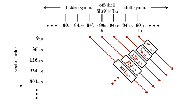
Figure 1: Minimal couplings (3.10) induced by different components of the embedding tensor $\Theta_{{\cal M}}$.

With the representation content (3.1), (3.12) and the minimal couplings (3.10), (3.11), one can read off the structure of the gauge algebra, i.e. identify the global symmetry generators that are promoted to local gauge symmetry. The couplings induced by choosing an embedding tensor in a given sub-representation of (3.12) are schematically depicted in figure 1, organized w.r.t. the respective charges under the derivation ${\bf d}$. Every diagonal line in the figure corresponds to the components of the embedding tensor at a given charge, and indicates the induced couplings between vector fields and symmetry generators. E.g. a gauging induced by the lowest component $\theta^{k}$ transforming in the ${\bf 9}^{\prime}_{-14/9}$ does not trigger any gauging of the off-shell symmetries of the Lagrangian. Rather it corresponds to the massive deformation discussed in (3.14) above. On-shell however, figure 1 shows that this deformation induces a gauging of some of the generators in the ${\bf 80}_{+1}$ corresponding to the on-shell shift symmetries (2.25) (as well as a gauging of the Virasoro generator ${\bf L}_{1}$ acting as a shift on the dual dilaton (2.22)).

The theory which we will construct in this paper is induced by an embedding tensor $\theta_{kl}=\theta_{(kl)}$ transforming in the ${\bf 45}_{-2/9}$ from the fifth level of (3.12). Figure 1 shows that these components induce a gauging of generators within the off-shell $SL(9)$ coupled to the vector fields $A_{\mu}{}^{kl}$ from (LABEL:susyvec). In contrast, none of the — potentially possible — generators from the ${\bf 84^{\prime}}_{-1/3}$ and ${\bf 84}_{+1/3}$ are involved in this gauging, as there are forbidden by the structure of representations: no ${\bf 45^{\prime}}$ appears in the tensor products ${\bf 9}\otimes{\bf 84^{\prime}}$ and ${\bf 126}\otimes{\bf 84}$ as would be required for such couplings to take place. For the same reason, the central charge generator ${K}$ is not gauged in this theory. More explicitly, the induced gauged subalgebra of $\mathfrak{sl}_{9}$ is generated by

$$X_{kl} \equiv \theta_{m[k}\,T_{l]}{}^{m}\;,$$ (3.15)

with the traceless $T_{k}{}^{l}$ denoting the generators of $\mathfrak{sl}_{9}$. A quick calculation confirms [42] that the resulting algebra is given by $\mathfrak{cso}_{p,q,r}$ (non-semisimple for $r>0$) with the integers $p+q+r=9$ characterizing the signature of $\theta_{kl}$. In particular — and this will be the theory of most interest in the following — choosing $\theta_{kl}\equiv\delta_{kl}$ amounts to gauging the full compact $\mathfrak{so}(9)\subset\mathfrak{sl}_{9}$. Figure 1 indicates that the full gauge algebra of the theory is given by an infinite-dimensional Borel subalgebra of $\mathfrak{e}_{9(9)}$ of which however all but a finite number of generators (that correspond to the compact $\mathfrak{so}(9)$) do not act on the physical fields and are only visible as shift symmetries on the infinite tower of dual scalar potentials, à la (2.25).

In general, the gauging defined by an embedding tensor according to (3.10) is consistent only in case the embedding tensor satisfies an additional quadratic constraint which in two dimensions takes the form

$$\Theta_{{\cal M}}{}^{{\cal A}}\,\Theta_{{\cal N}}{}^{{\cal B}}\,\eta_{{\cal AB}}~{}=~{}0\qquad\Longleftrightarrow\qquad\eta^{{\cal A}{\cal B}}\,T_{{\cal A},{\cal M}}{}^{{\cal P}}\,T_{{\cal B},{\cal N}}{}^{{\cal Q}}\,\Theta_{{\cal P}}\Theta_{{\cal Q}}~{}=~{}0\;.$$ (3.16)

It has been shown in [24] that an embedding tensor transforming in the ${\bf 45}_{-2/9}$ as considered above, automatically satisfies the quadratic constraint (3.16), i.e. any choice of $\theta_{kl}$ defines a consistent gauging. We will confirm that statement in this paper by explicit construction. A first indication is the fact that for any choice of $\theta_{kl}$, the projected generators (3.15) close into an algebra.

To summarize, the structure of the gauged theory constructed in this paper follows from the general representation structure of vector fields and embedding tensor components. We will thus consider a deformation of the Lagrangian (2.10), whose local gauge algebra is given by the subalgebra of the global $\mathfrak{sl}_{9}$ spanned by the generators (3.15). This is realized by introducing minimal couplings via the covariant derivatives

$${\cal D}_{\mu} = \partial_{\mu}-gA_{\mu}{}^{kl}\,\theta_{mk}\,T_{l}{}^{m}\;,$$ (3.17)

with the vector fields $A_{\mu}{}^{kl}=A_{\mu}{}^{[kl]}$ from (LABEL:susyvec). In the following we will absorb the explicit coupling constant $g$ by rescaling $\theta_{mk}$. In the next section, we will give the details of this construction and show in particular, that it is compatible with maximal supersymmetry.

4 SO(9) supergravity: the Lagrangian

Having discussed maximal supergravity in two dimensions in the appropriate $SL(9)$ covariant formulation, we proceed to the construction of the gauged theory, i.e. in the following we gauge the compact $SO(9)$ subgroup of the global symmetry (2.13). Just as to avoid any confusion, let us stress that the resulting theory possesses two local $SO(9)$ symmetries. The first, which for distinctiveness we shall refer to as $SO(9)_{K}$ is simply related to the $SL(9)/SO(9)$ coset formulation (2.8) and already present in the ungauged theory discussed above. It acts linearly on the fermions and on the scalar fields ${\cal V}$ by right multiplication

$$\delta{\cal V}_{k}{}^{a} = {\cal V}_{k}{}^{b}\,\Omega^{[ba]}\;.$$ (4.1)

On the other hand , the new gauge symmetry $SO(9)_{\rm gauge}$ to be introduced in the following acts by left multiplication on the scalars ${\cal V}$ and rotates the 84 scalars $\phi^{klm}$ according to (2.13). Fully covariant derivatives carry the composite connection $Q_{\mu}^{ab}$ from (2.8) w.r.t. $SO(9)_{K}$ and the connection (3.17) w.r.t. $SO(9)_{\rm gauge}$.

4.1 General ansatz

In a first step, we introduce minimal couplings according to (3.17) in order to ensure invariance of the Lagrangian under local gauge transformations generated by (3.15). Eventually, we will set $\theta_{kl}\equiv\delta_{kl}$ such that the gauge group corresponds to the maximal compact subgroup $SO(9)$ of (2.13). Throughout the construction it turns out to be helpful to keep an arbitrary $\theta_{kl}$ for bookkeeping of the different terms. As a byproduct, the very same construction also yields the theories with $SO(p,9-p)$ and non-semisimple $CSO(p,q,9-p-q)$ gauge groups, according to the choice of $\theta_{kl}$.

The general ansatz for the gauged Lagrangian then is the following deformation of (2.10):

$${\cal L} = {\cal L}_{0,{\rm cov}}-\frac{1}{4}\,\varepsilon^{\mu\nu}{{\cal{F}}_{\mu\nu}}{}^{kl}{}\theta_{lm}\,{Y_{k}}^{m}+{\cal L}_{\rm Yuk}+{\cal L}_{\rm pot}\;,$$ (4.2)

where ${\cal L}_{0,{\rm cov}}$ is obtained by straightforward covariantization of (2.10) according to

$$Q_{\mu}^{[ab]}+P_{\mu}^{(ab)} \rightarrow {\cal Q}_{\mu}^{[ab]}+{\cal P}_{\mu}^{(ab)}~{}\equiv~{}{\cal{V}}^{-1}{}^{ak}\,\left(\partial_{\mu}{{\cal{V}}_{k}}^{b}-A_{\mu}{}^{lm}\theta_{mk}\,{{\cal{V}}_{l}}^{b}\right)\;,$$

$$\partial_{\mu}\phi^{klm} \rightarrow {\cal D}_{\mu}\phi^{klm}~{}\equiv~{}\partial_{\mu}\phi^{klm}-3\,A_{\mu}{}^{p[k}\theta_{pq}\,\phi^{lm]q}\;,$$

$${\varphi}_{\mu}^{abc} \rightarrow \widetilde{\varphi}_{\mu}^{abc}~{}\equiv~{}{{\cal{V}}_{klm}}^{[abc]}\,{\cal D}_{\mu}\phi^{klm}\;,$$

$$D_{\mu}\psi_{\nu}^{I} \rightarrow {\cal D}_{\mu}\psi_{\nu}^{I}~{}\equiv~{}\partial_{\mu}\psi_{\nu}^{I}+\frac{1}{4}{{\omega_{\mu}}^{\alpha\beta}}\gamma_{\alpha\beta}\,\psi_{\nu}^{I}+\frac{1}{4}{\cal Q}_{\mu}^{ab}\,\Gamma_{IJ}^{ab}\,\psi_{\nu}^{J}\;,$$

$$D_{\mu}\chi^{aI} \rightarrow {\cal D}_{\mu}\chi^{aI}~{}\equiv~{}\partial_{\mu}\chi^{aI}+\frac{1}{4}{{\omega_{\mu}}^{\alpha\beta}}\gamma_{\alpha\beta}\,\chi^{aI}+{\cal Q}_{\mu}^{ab}\,\chi^{bI}+\frac{1}{4}{\cal Q}_{\mu}^{bc}\,\Gamma_{IJ}^{bc}\,\chi^{aJ}\;,$$ (4.3)

and thus gauge invariant by construction. Furthermore,

$${\cal F}_{\mu\nu}{}^{kl} \equiv 2\partial_{[\mu}A_{\nu]}{}^{kl}+2\,\theta_{pq}\,A_{[\mu}{}^{p[k}A_{\nu]}{}^{l]q}\;,$$ (4.4)

defines the non-abelian field strength of the vectors $A_{\mu}{}^{kl}=A_{\mu}{}^{[kl]}$ which in (4.2) couples to an auxiliary field ${Y_{k}}^{l}$. In anticipation of the final structure we denote this auxiliary field by the same letter as the dual scalar potential defined in (2.15) above for the ungauged theory. The general ansatz for the Yukawa-type couplings ${\cal L}_{\rm Yuk}$ in (4.2) is the collection of the most general bilinear fermion couplings

$$e^{-1}{\cal L}_{\rm Yuk} = -\frac{1}{2}\,e^{-1}\rho\,\varepsilon^{\mu\nu}\left(\bar{\psi}_{\nu}^{I}\psi_{\mu}^{J}B_{IJ}+\bar{\psi}_{\nu}^{I}\gamma^{3}\psi_{\mu}^{J}\tilde{B}_{IJ}-2i\bar{\psi}_{2}^{I}\gamma_{\nu}\psi_{\mu}^{J}A_{IJ}\right)+i\rho\,\bar{\psi}_{2}^{I}\gamma^{\mu}\psi_{\mu}^{J}\tilde{A}_{IJ}$$ (4.5)

$${}+i\rho\,\bar{\chi}^{aI}\gamma^{\mu}\psi_{\mu}^{J}C^{a}_{IJ}\;-i\rho\,\bar{\chi}^{aI}\gamma^{3}\gamma^{\mu}\psi_{\mu}^{J}\tilde{C}^{a}_{IJ}\;+\rho\,\bar{\psi}_{2}^{I}\psi_{2}^{J}D_{IJ}\;+\rho\,\bar{\psi}_{2}^{I}\gamma^{3}\psi_{2}^{J}\tilde{D}_{IJ}$$

$${}+\rho\,\bar{\chi}^{aI}\psi_{2}^{J}E_{IJ}^{a}\;+\rho\,\bar{\chi}^{aI}\gamma^{3}\psi_{2}^{J}\tilde{E}_{IJ}^{a}\;+\rho\,\bar{\chi}^{aI}\chi^{bJ}F_{IJ}^{ab}\;+\rho\,\bar{\chi}^{aI}\gamma^{3}\chi^{bJ}\tilde{F}_{IJ}^{ab}\;,$$

with tensors $A$, $B$, $C$, $D$, $E$, $F$, depending on the scalar and auxiliary fields to be determined in the following. Their appearance in (4.5) implies certain symmetry properties such as

$$B_{(IJ)}=\tilde{D}_{(IJ)}=0=\tilde{B}_{[IJ]}=D_{[IJ]}\;,\qquad F_{IJ}^{ab}=F_{JI}^{ba}\;,\qquad\tilde{F}_{IJ}^{ab}=-\tilde{F}_{JI}^{ba}\;,$$ (4.6)

and

$$\Gamma_{IJ}^{a}C_{IK}^{a}=\Gamma_{IJ}^{a}\tilde{C}_{IK}^{a}=0\;.$$ (4.7)

As is standard in gauged supergravity, couplings of the type (4.5) induce a modification of the fermionic supersymmetry transformation rules (2.12) by introduction of the so-called fermion shifts according to

$$\delta_{\epsilon}\psi_{\mu}^{I} = {\cal D}_{\mu}\epsilon^{I}-\frac{1}{24}\,\rho^{-1/3}\Gamma_{IJ}^{abc}\Big{(}\gamma^{\nu}\gamma_{\mu}+\frac{1}{3}\gamma_{\mu}\gamma^{\nu}\Big{)}\gamma^{3}\epsilon^{J}\,\widetilde{\varphi}_{\nu}^{abc}+i\left(A_{IJ}+\tilde{A}_{IJ}\gamma^{3}\right)\gamma_{\mu}\epsilon^{J}\;,$$

$$\delta_{\epsilon}\psi_{2}^{I} = -\frac{i}{2}\,\rho^{-1}\left(\partial_{\mu}\rho\right)\gamma^{3}\gamma^{\mu}\epsilon^{I}+\left(B_{IJ}+\tilde{B}_{IJ}\,\gamma^{3}\right)\epsilon^{J}\;,$$

$$\delta_{\epsilon}\chi^{aI} = \frac{i}{2}\,\Gamma_{IJ}^{b}\,\gamma^{\mu}\epsilon^{J}{\cal P}_{\mu}^{ab}-\frac{i}{6}\,\rho^{-{1/3}}\Big{(}\delta^{ad}\Gamma_{IJ}^{bc}-\frac{1}{6}\,\Gamma_{IJ}^{abcd}\Big{)}\,\gamma^{3}\gamma^{\mu}\epsilon^{J}\,\widetilde{\varphi}_{\mu}^{bcd}+\left(C^{a}_{IJ}+\tilde{C}^{a}_{IJ}\gamma^{3}\right)\epsilon^{J}\;,$$

with the scalar-dependent tensors $A$, $B$, $C$ parametrizing (4.5). The bosonic supersymmetry transformation rules from (2.12) remain unchanged, the vector fields transform as determined in (LABEL:susyvec)

$$\delta_{\epsilon}\,A_{\mu}{}^{kl} = \rho^{-2/9}\Big{(}\bar{\psi}_{\mu}^{I}\epsilon^{J}\Gamma_{IJ}^{ab}-\frac{2i}{9}\,\bar{\psi}_{2}^{I}\gamma^{3}\gamma_{\mu}\epsilon^{J}\Gamma_{IJ}^{ab}-2i\,\bar{\chi}^{I[a}\gamma_{\mu}\epsilon^{J}\Gamma_{IJ}^{b]}\Big{)}{\cal{V}}^{-1}{}_{[ab]}{}^{kl}$$ (4.9)

$${}+2\,\rho^{-5/9}\Big{(}\bar{\psi}_{\mu}^{I}\gamma^{3}\epsilon^{J}\Gamma_{IJ}^{a}+\frac{5i}{9}\,\bar{\psi}_{2}^{I}\gamma_{\mu}\epsilon^{J}\Gamma_{IJ}^{a}-i\bar{\chi}^{aI}\gamma^{3}\gamma_{\mu}\epsilon^{I}\Big{)}{\cal{V}}^{-1}{}_{[bc]}{}^{kl}\,\varphi^{abc}\;,$$

and the transformation of the auxiliary scalar fields $Y_{k}{}^{l}$ is described by (4.14) below. Finally, ${\cal L}_{\rm pot}$ in (4.2) describes a scalar potential whose form is most conveniently deduced by demanding the absence of terms proportional to $\bar{\psi}^{I}_{\mu}\gamma^{\mu}\epsilon^{I}$ in the supersymmetry variation of the full Lagrangian (4.2):

$${\cal L}_{\rm pot} \equiv -eV_{\rm pot}~{}=~{}-\frac{1}{16}\,e\rho\left(2\tilde{A}_{IJ}B_{IJ}-2A_{IJ}\tilde{B}_{IJ}+C_{IJ}^{a}C_{IJ}^{a}+\tilde{C}_{IJ}^{a}\tilde{C}_{IJ}^{a}\right)\;,$$ (4.10)

in terms of the Yukawa tensors. The entire Lagrangian (4.2) with (4.5), (4.10) thus is given as a function of the scalar functions, $A$, $B$, $C$, $D$, $E$, $F$, which we will determine explicitly in the next section as functions of the scalar and auxiliary fields. Before diving into that calculation, let us finish this section by commenting on the supersymmetry transformations of the vector and auxiliary fields $A_{\mu}{}^{kl}$ and $Y_{k}{}^{l}$, respectively. These have been added as new fields in (4.2) and do not appear in the ungauged theory (2.10).

The role of the vector fields has been discussed in section 3 above: the underlying affine symmetry structure predicts to employ for this gauging 36 vector fields $A_{\mu}{}^{kl}$ in a finite sub-representation of the basic representation (3.1) of $\mathfrak{e}_{9(9)}$ . We have determined their supersymmetry transformation rules in (LABEL:susyvec), (4.9) by demanding closure of the supersymmetry algebra. As for the auxiliary fields $Y_{k}{}^{l}$, their structure is even more restricted. When checking supersymmetry of the gauged Lagrangian (4.2), the result of the ungauged theory (2.10) is modified by the presence of the gauge connections as a result of which covariant derivatives no longer commute:

$$[{\cal D}_{\mu},{\cal D}_{\nu}]\;\phi^{klm} = -3\,\theta_{pq}\,{\cal F}_{\mu\nu}{}^{p[k}\,\phi^{lm]q}\;,$$

$${\cal D}^{\vphantom{a}}_{[\mu}\,{\cal P}^{ab}_{\nu]} = \frac{1}{2}\,\theta_{kl}\,{\cal V}_{m(a}\,{\cal V}^{-1}{}_{b)}{}^{k}\,{\cal F}_{\mu\nu}{}^{lm}\;,$$ (4.11)

etc.. Variation of ${\cal L}_{0,{\rm cov}}$ thus leads to a number of terms proportional to the field strength ${\cal F}_{\mu\nu}{}^{kl}$ which we collect as

$$\delta_{\epsilon}\,{\cal L}_{0,{\rm cov}} = \frac{1}{4}\varepsilon^{\mu\nu}{{\cal{F}}_{\mu\nu}}{}^{kl}{}\theta_{lm}\;{\Xi_{k}}^{m}\;,$$ (4.12)

up to total derivatives, with

$${\Xi_{k}}^{l} = \bar{\chi}^{aI}\gamma^{3}\varepsilon^{J}\left(-\rho\,{{\cal{V}}_{k}}^{(a}{\cal{V}}^{-1}{}^{b)l}\,\Gamma_{IJ}^{b}+{\frac{1}{3}\,\rho^{1/3}\,{{\cal{V}}_{k}}^{g}{\cal{V}}^{-1}{}^{jl}\,\delta^{a[d}\Gamma_{IJ}^{efghi]}\,\varphi^{def}\varphi^{hij}}\right)$$ (4.13)

$${}+\frac{3}{2}\,\rho^{2/3}\,\bar{\chi}^{aI}\varepsilon^{J}\,{\cal{V}}^{-1}{}^{gl}{{\cal{V}}_{k}}^{[a}\varphi^{bc]g}\,\Gamma_{IJ}^{bc}+\frac{1}{3}\,\rho^{2/3}\,\bar{\psi}_{2}^{I}\gamma^{3}\varepsilon^{J}\,{\cal{V}}^{-1}{}^{gl}{{\cal{V}}_{k}}^{a}\varphi^{bcg}\,\Gamma_{IJ}^{abc}$$

$${}+\bar{\psi}_{2}^{I}\varepsilon^{J}\left({\frac{1}{2}}\rho\,{\cal{V}}^{-1}{}^{al}{{\cal{V}}_{k}}^{b}\,\Gamma_{IJ}^{ab}+\frac{1}{54}\,\rho^{1/3}\,{\cal{V}}^{-1}{}^{gl}{{\cal{V}}_{k}}^{d}\,\varphi^{abc}\varphi^{efg}\,\Gamma_{IJ}^{abcdef}\right)\;.$$

The role of the new coupling of the field strength to an auxiliary field $Y_{k}{}^{l}$ in (4.2) is precisely to cancel the unwanted contributions (4.12) by imposing

$$\delta_{\epsilon}\,Y_{k}{}^{l} = {\Xi_{k}}^{l}\;.$$ (4.14)

Comparing (4.13) to (2.16), we deduce, that we may identify the auxiliary field $Y_{k}{}^{l}$ with the dual scalar potential defined in (2.15) for the ungauged theory. Moreover, the vector field equations of the full Lagrangian (4.2) give rise to the duality equations

$$-e\varepsilon_{\mu\nu}\theta_{m[k}{\cal D}^{\nu}Y_{l]}{}^{m} = \rho\,\theta_{m[k}{{\cal{V}}_{l]a}}{\cal{V}}^{-1}{}_{b}{}^{m}\left({\cal P}_{\mu}^{ab}-\rho^{-2/3}\,\varphi^{bcd}\widetilde{\varphi}_{\mu}^{acd}\right)$$ (4.15)

$${}+\frac{1}{54}\,e\varepsilon_{\mu\nu}\,\varepsilon^{abcdefghi}\,\theta_{m[k}{{\cal{V}}_{l]}}^{a}{\cal{V}}^{-1}{}^{jm}\,\varphi^{bcj}\varphi^{def}\widetilde{\varphi}^{\nu\,ghi}$$

$${}+~{}{\rm fermions}\;,$$

which can be understood as the proper covariantization of (a projected version of) the duality equations (2.15) of the ungauged theory.

To summarize, the supersymmetry transformation rules of the various fields appearing in the gauged theory are given in (2.12), (LABEL:susyshift), (4.9), and (4.14). The Lagrangian is of the form (4.2) with (4.5) and (4.10) given in terms of the scalar functions, $A$, $B$, $C$, $D$, $E$, $F$, that we will determine explicitly in the next section.

4.2 Yukawa tensors

With the general ansatz for the Lagrangian specified in (4.2), (4.5), (4.10), we are now in position to explicitly check its transformation under supersymmetry using (2.12), (LABEL:susyshift), (4.9), and (4.14). As a first result, we obtain a number of linear relations among the Yukawa tensors $A$, $B$, $C$, $D$, $E$, $F$ by demanding that all terms linear in space-time derivatives cancel in the supersymmetry variation of (4.2). E.g. vanishing of the terms proportional to $\bar{\psi}_{\mu}^{I}\gamma^{\mu\nu}\epsilon^{J}\,\partial_{\nu}\rho$ and $\bar{\chi}^{aI}\gamma^{\mu}\epsilon^{J}\,\partial_{\mu}\rho$ imposes the relations

$$A_{IJ}-\tilde{B}_{IJ}-\rho\frac{\delta\tilde{B}_{IJ}}{\delta\rho} = 0\;,$$

$$C^{a}_{IJ}+2\rho\frac{\delta{C}^{a}_{IJ}}{\delta\rho}+\tilde{E}^{a}_{IJ} = 0\;,$$ (4.16)

respectively. A more complete list of all such linear relations is collected in appendix A.1. Upon decomposing the Yukawa tensors into their $SO(9)_{K}$ irreducible parts, we find that they are uniquely determined by these linear relations in terms of the scalar fields ${\cal V}_{k}{}^{a}$, $\Phi^{klm}$ and the auxiliary fields $Y_{k}{}^{l}$ . The final result is obtained after some lengthy calculation and reads

$$A_{IJ} = \frac{7}{9}\,\delta_{IJ}\,b-\frac{5}{9}\,\Gamma_{IJ}^{a}\,b^{a}{-}\frac{1}{9}\,\Gamma_{IJ}^{abcd}\,b^{abcd}\;,$$

$$\tilde{A}_{IJ} = {-}\frac{2}{9}\,\Gamma_{IJ}^{ab}\,b^{ab}{-}\frac{4}{9}\,\Gamma_{IJ}^{abc}\,b^{abc}\;,$$

$$B_{IJ} = {-}\Gamma_{IJ}^{ab}\,b^{ab}{-}\Gamma_{IJ}^{abc}\,b^{abc}\;,$$

$$\tilde{B}_{IJ} = \delta_{IJ}\,b+\Gamma_{IJ}^{a}\,b^{a}{-}\Gamma_{IJ}^{abcd}\,b^{abcd}\;,$$

$$C_{IJ}^{a} = \frac{8}{9}\,\delta_{IJ}\,b^{a}-\frac{1}{9}\Gamma_{IJ}^{ab}\,b^{b}{-}\frac{20}{9}\,\Gamma_{IJ}^{bcd}\,b^{abcd}{+}\frac{4}{9}\,\Gamma_{IJ}^{abcde}\,b^{bcde}+{c}^{ab}\,\Gamma_{IJ}^{b}\;,$$

$$\tilde{C}_{IJ}^{a} = {+}\frac{14}{9}\,\Gamma_{IJ}^{b}\,b^{ab}{-}\frac{2}{9}\,\Gamma_{IJ}^{abc}\,b^{bc}{-}\frac{2}{3}\,\Gamma_{IJ}^{bc}\,b^{abc}{+}\frac{1}{9}\,\Gamma_{IJ}^{abcd}\,b^{bcd}+{c}^{a,bc}\,\Gamma_{IJ}^{bc}\;,$$

$$D_{IJ} = \frac{14}{81}\,\delta_{IJ}\,b-\frac{70}{81}\,\Gamma_{IJ}^{a}\,b^{a}{-}\frac{8}{81}\,\Gamma_{IJ}^{abcd}\,b^{abcd}\;,$$

$$\tilde{D}_{IJ} = {-}\frac{22}{81}\,\Gamma_{IJ}^{ab}\,b^{ab}{+}\frac{20}{81}\,\Gamma_{IJ}^{abc}\,b^{abc}\;,$$

$$E_{IJ}^{a} = {-}\frac{26}{9}\,\Gamma_{IJ}^{b}\,b^{ab}{+}\frac{1}{9}\,\Gamma_{IJ}^{bc}\,b^{abc}-\frac{1}{9}\,{c}^{a,bc}\,\Gamma_{IJ}^{bc}\;,$$

$$\tilde{E}_{IJ}^{a} = \frac{19}{9}\,\delta_{IJ}\,b^{a}{-}\frac{28}{9}\,\Gamma_{IJ}^{bcd}\,b^{abcd}-\frac{5}{9}\,{c}^{ab}\,\Gamma_{IJ}^{b}\;,$$

$$F^{ab}_{IJ} = -\frac{1}{18}\,\delta^{ab}\delta_{IJ}\,b+\frac{1}{2}\,\delta^{ab}\,\Gamma_{IJ}^{c}\,b^{c}{+}\frac{1}{2}\,\delta^{ab}\,\Gamma_{IJ}^{cdef}\,b^{cdef}-12\,\Gamma_{IJ}^{cd}\,b^{abcd}-2\,{c}^{ab}\,\delta_{IJ}\;,$$

$$\tilde{F}^{ab}_{IJ} = {-}\frac{1}{2}\,\delta^{ab}\,\Gamma_{IJ}^{cd}\,b^{cd}{+}\frac{1}{2}\,\delta^{ab}\,\Gamma_{IJ}^{cde}\,b^{cde}{+}2\,\delta_{IJ}\,b^{ab}{+}2\,\Gamma_{IJ}^{c}\,b^{abc}-2\,{c}^{c,ab}\,\Gamma_{IJ}^{c}\;,$$ (4.17)

expressed in terms of the $SO(9)_{K}$ irreducible tensors

$$b = \frac{1}{4}\,\rho^{-2/9}\,T\;,$$

$$b^{a} = -\rho^{-14/9}\,T^{cd}\,\varphi^{abc}{\cal Y}^{bd}+\frac{1}{144}\,\rho^{-14/9}\,\varepsilon^{bcdefghij}T^{kl}\varphi^{kef}\varphi^{lgh}\varphi^{aij}\varphi^{bcd}\;,$$

$$b^{ab} = -\frac{1}{2}\,\rho^{-11/9}\,T^{d[a}{\cal Y}^{b]d}+\frac{1}{144}\,\rho^{-11/9}\,\varepsilon^{abcdefghi}T^{jk}\varphi^{jcd}\varphi^{kef}\varphi^{ghi}\;,$$

$$b^{abc} = \frac{1}{4}\,\rho^{-5/9}\,T^{d[a}\varphi^{bc]d}\;,$$

$$b^{abcd} = -\frac{1}{8}\,\rho^{-8/9}\,T^{ef}\varphi^{e[ab}\varphi^{cd]f}\;,$$

$${c}^{ab} = -\frac{1}{2}\,\rho^{-2/9}\Big{(}T^{ab}-\frac{1}{9}\delta^{ab}T\Big{)}\;,$$

$${c}^{a,bc} = \frac{1}{3}\,\rho^{-5/9}\left(T^{da}\varphi^{bcd}-T^{d[b}\varphi^{c]ad}\right)\;,$$ (4.18)

where we have defined

$$T^{ab} \equiv {\cal{V}}^{-1}{}^{(kl)}{}_{ab}\,\theta_{kl}\;,\quad T~{}\equiv~{}T^{aa}\;,\quad$$

$$\varphi^{abc} \equiv {\cal V}_{[klm]}{}^{abc}\phi^{klm}\;,\quad{\cal Y}^{ab}~{}\equiv~{}{\cal V}^{-1}{}^{ak}\,{\cal V}_{l}{}^{b}\,Y_{k}{}^{l}\;.$$ (4.19)

It may seem remarkable, that the highly overdetermined system (A.1)–(A.4) of linear relations for the Yukawa tensors admits a non-trivial solution (4.17), (4.18). With hindsight, this is a further confirmation that the algebraic framework which determines the gauge couplings based on the underlying affine symmetry [24] is indeed compatible with supersymmetry.

A further (and final) test to the construction comes from vanishing of the terms that are bilinear in $\theta_{kl}$ in the supersymmetry variation of (4.2). E.g. cancellation of the terms proportional to $\bar{\psi}^{I}_{\mu}\gamma^{\mu}\gamma^{3}\epsilon^{J}$ implies the relation

$$2A_{K(I}B_{J)K}+2\tilde{A}_{K(I}\tilde{B}_{J)K}+C^{a}_{KI}\tilde{C}^{a}_{KJ}+C^{a}_{KJ}\tilde{C}^{a}_{KI} = 0\;.$$ (4.20)

Employing the linear constraints (A.1) this relation reduces to

$$\left(4+2\rho\partial\rho\right)(B_{K(I}\tilde{B}_{J)K})=C^{a}_{KI}\tilde{C}^{a}_{KJ}+C^{a}_{KJ}\tilde{C}^{a}_{KI}$$

With the explicit parametrization (4.17) in terms of $SO(9)_{K}$ irreducible tensors, the l.h.s. and r.h.s. of this equation become

$$\left(4+2\rho\partial\rho\right)(B_{K(I}\tilde{B}_{J)K}) = \Gamma^{b}_{IJ}\left(\frac{80}{3}\,b^{def}b^{defb}-\frac{28}{9}\,b^{a}b^{ab}\right)+\frac{2}{9}\,\Gamma^{aefg}_{IJ}\left(8\,b^{ab}b^{befg}-b^{a}b^{efg}\right)$$

$${}-\frac{40}{3}\,\Gamma^{abefg}_{IJ}\,b^{abc}b^{cefg}\;,$$

$$C^{a}_{KI}\tilde{C}^{a}_{KJ}+C^{a}_{KJ}\tilde{C}^{a}_{KI} = \Gamma^{b}_{IJ}\left(\frac{80}{3}\,b^{def}b^{defb}-\frac{28}{9}\,b^{a}b^{ab}\right)+\frac{2}{9}\,\Gamma^{aefg}_{IJ}\left(8\,b^{ab}b^{befg}-b^{a}b^{efg}\right)$$

$${}+\Gamma^{abefg}_{IJ}\left(\frac{8}{3}\,b^{abc}b^{cefg}-8\,c^{c,ab}b^{cefg}\right)\;,$$

respectively. Eventually, the quadratic relation (4.20) thus boils down to the relation

$$c^{f,[ab}b^{cde]f} = 2\,b^{f[ab}b^{cde]f}\;,$$ (4.21)

for the tensors $b^{abc}$, $b^{abcd}$, $c^{a,bc}$. With the explicit form (4.18) of these tensors, it is straightforward to verify, that this equation is indeed identically satisfied.

Supersymmetry imposes several other quadratic conditions analogous to (4.20) on the Yukawa tensors, which we have collected in appendix A.2. Just as for (4.20), straightforward but lengthy computation shows that all these quadratic equations are identically satisfied with the explicit form (4.17), (4.18) of the Yukawa tensors. This completes the main result of this section: the Lagrangian (4.2) with (4.5), (4.10) and the Yukawa tensors given in (4.17), (4.18) above is maximally supersymmetric (up to higher fermion terms and total derivatives). This result confirms the prediction of [24] discussed in section 3.2 above that any embedding tensor $\theta_{kl}$ defines a consistent gauged theory compatible with maximal supersymmetry. In the following, we will set $\theta_{kl}=g\delta_{kl}$ thereby specifying the construction to the $SO(9)$ theory while making the gauge coupling constant manifest. Accordingly, we use the $\delta_{kl}$ symbol to raise and lower the corresponding indices.

Let us finally note that with the Yukawa tensors determined in terms of the scalar fields, we may evaluate the scalar potential (4.10) of the theory and obtain

$${V}_{\rm pot} = \rho\Big{(}2\,b^{a}b^{a}+4\,b^{ab}b^{ab}+48\,b^{abcd}b^{abcd}+{c}^{ab}{c}^{ab}+2\,{c}^{a,bc}\,{c}^{a,bc}-\frac{14}{9}\,bb-4\,b^{abc}b^{abc}\Big{)}\;,$$

in terms of the $SO(9)_{K}$ irreducible tensors (4.18).

4.3 Supersymmetry algebra

Having shown that the Lagrangian (4.2) defines a maximally supersymmetric theory with local gauge group $SO(9)$, it is instructive to analyze the structure of the supersymmetry algebra of this model. On the bosonic fields appearing in (2.10), the supersymmetry algebra closes in a standard fashion

$$[\delta_{\epsilon_{1}},\delta_{\epsilon_{2}}] = \xi^{\mu}\,{\cal D}_{\mu}+\delta^{\rm Lorentz}_{\omega}+\delta^{SO(9)_{K}}_{\Omega}+\delta^{SO(9)_{\rm gauge}}_{\Lambda}\;,$$ (4.23)

into the local bosonic symmetries of the gauged theory. As usual, $\xi^{\mu}\,{\cal D}_{\mu}$ denotes a covariant general coordinate transformation with parameter $\xi^{\mu}$, combining a spacetime diffeomorphism with the gauge transformations of the form

$$\omega^{\alpha\beta}=-\xi^{\mu}\omega_{\mu}{}^{\alpha\beta}\;,\quad\Omega^{ab}=-\xi^{\mu}{\cal Q}_{\mu}^{ab}\;,\quad\Lambda^{kl}=-\xi^{\mu}A_{\mu}{}^{kl}\;.$$ (4.24)

The r.h.s. of the supersymmetry algebra (4.23) is given by gauge transformations with parameters

$$\xi^{\mu} = i\,\bar{\epsilon}_{2}^{I}\gamma^{\mu}\epsilon_{1}^{I}\;,$$

$$\omega^{\alpha\beta} = -2\,\varepsilon^{\alpha\beta}\left(\bar{\epsilon}_{2}^{I}\gamma^{3}\epsilon_{1}^{J}A_{IJ}-\bar{\epsilon}_{2}^{I}\epsilon_{1}^{J}\tilde{A}_{IJ}\right)\;,$$

$$\Lambda^{kl} = -\rho^{-5/9}\,{\cal{V}}^{-1}{}_{[ab]}{}^{kl}\left(\rho^{1/3}\,\bar{\epsilon}_{2}^{I}\epsilon_{1}^{J}\Gamma_{IJ}^{ab}\,+2\,\bar{\epsilon}_{2}^{I}\gamma^{3}\epsilon_{1}^{J}\,\Gamma_{IJ}^{c}\,\varphi^{abc}\right)\;,$$

$$\Omega^{ab} = -\Lambda^{kl}\,{\cal V}_{kl}{}^{c[a}\,T^{b]c}\;.$$ (4.25)

Closure of the supersymmetry algebra requires several of the identities among the Yukawa tensors that we have collected in appendix A, as well as their explicit form (4.17). E.g. evaluating successive supersymmetry transformations on the scalars ${\cal V}_{k}{}^{a}$ yields

$$[\delta_{\epsilon_{1}},\delta_{\epsilon_{2}}]\,{{\cal{V}}_{m}}^{a} = \xi^{\mu}\,{\cal P}_{\mu}{{\cal{V}}_{m}}^{a}+\lambda^{(ab)}\,{{\cal{V}}_{m}}^{b}\;,$$ (4.26)

with

$$\lambda^{(ab)} \equiv 2\,\left(\bar{\epsilon}_{2}^{I}\gamma^{3}\epsilon_{1}^{J}\,\tilde{C}_{K(I}^{(a}\Gamma_{J)K}^{b)}-\bar{\epsilon}_{2}^{I}\epsilon_{1}^{J}\,C_{K[I}^{(a}\Gamma_{J]K}^{b)}\right)$$ (4.27)

$$= 2\,\rho^{-5/9}\,\bar{\epsilon}_{2}^{I}\gamma^{3}\epsilon_{1}^{J}\,\Gamma_{IJ}^{c}\,T^{d(a}\varphi^{b)cd}+\rho^{-2/9}\,\bar{\epsilon}_{2}^{I}\epsilon_{1}^{J}\,\Gamma^{c(a}T^{b)c}$$

$$= \Lambda^{ml}\theta_{kl}{\cal V}_{m}{}^{a}{\cal V}^{-1\,kb}-\Omega^{ab}\;,$$

such that the second term in (4.26) may be rewritten

$$\lambda^{(ab)}\,{{\cal{V}}_{m}}^{b} = \Lambda^{kl}\theta_{lm}{\cal V}_{k}{}^{a}+{{\cal{V}}_{m}}^{b}\,\Omega^{ba}\;,$$ (4.28)

as a combination of local $SO(9)_{\rm gauge}$ and $SO(9)_{K}$ transformations with the parameters of (4.25). Moreover, we find that the parameter of gauge transformations $\Lambda^{kl}$ that arises in this commutator precisely agrees with what we have found in lowest order in the closure of the supersymmetry algebra on the vector fields in (3.8). When computing the algebra of the full supersymmetry transformations (LABEL:susyshift) on the vector fields, we obtain additional contributions from the fermion shifts

$$[\delta_{\epsilon_{1}},\delta_{\epsilon_{2}}]\,{A_{\mu}}^{kl} = {\cal D}_{\mu}\Lambda^{kl}+2i\rho^{-2/9}\,{\cal{V}}^{-1}{}^{kl}{}_{[ab]}\left(\bar{\epsilon}_{2}^{I}\gamma_{\mu}\epsilon_{1}^{J}\,Z^{ab}_{IJ}-\bar{\epsilon}_{2}^{I}\gamma^{3}\gamma_{\mu}\epsilon_{1}^{J}\,\tilde{Z}^{ab}_{IJ}\right)\;,$$ (4.29)

which upon using (A.1) and the explicit form (4.17), (4.18), of the Yukawa tensors combine into

$$Z^{ab}_{IJ} = 2C_{K(I}^{[a}\Gamma_{J)K}^{b]}-{\Big{(}A_{K(I}-\frac{2}{9}\tilde{B}_{K(I}\Big{)}\,\Gamma^{ab}_{J)K}-2\rho^{-1/3}\varphi^{abc}\Big{[}\tilde{C}_{(IJ)}^{c}+\Big{(}\tilde{A}_{K(I}+\frac{5}{9}B_{K(I}\Big{)}\Gamma_{J)K}^{c}\Big{]}}$$ (4.30)

$$= \Big{[}2C_{K(I}^{[a}\Gamma_{J)K}^{b]}-\Big{(}\frac{7}{9}+\rho\partial_{\rho}\Big{)}\,\tilde{B}_{K(I}\,\Gamma_{J)K}^{ab}\Big{]}-2\rho^{-1/3}\varphi^{abc}\Big{[}\tilde{C}_{(IJ)}^{c}-\Big{(}\frac{4}{9}+\rho\partial_{\rho}\Big{)}B_{K(I}\Gamma_{J)K}^{c}\Big{]}$$

$$= 0\;,$$

and

$$\tilde{Z}^{ab}_{IJ} = 2\tilde{C}_{K(I}^{[a}\Gamma_{J)K}^{b]}+{\Big{(}\tilde{A}_{K(I}+\frac{2}{9}B_{K(I}\Big{)}\Gamma_{J)K}^{ab}-2\rho^{-1/3}\varphi^{abc}\Big{[}C_{(IJ)}^{c}-\Big{(}A_{K(I}-\frac{5}{9}\tilde{B}_{K(I}\Big{)}\Gamma_{J)K}^{c}\Big{]}}$$ (4.31)

$$= \Big{[}2\tilde{C}_{K(I}^{[a}\Gamma_{J)K}^{b]}-\Big{(}\frac{7}{9}+\rho\partial_{\rho}\Big{)}{B}_{K(I}\Gamma_{J)K}^{ab}\Big{]}-2\rho^{-1/3}\varphi^{abc}\Big{[}C_{(IJ)}^{c}-\Big{(}\frac{4}{9}+\rho\partial_{\rho}\Big{)}\tilde{B}_{K(I}\Gamma_{J)K}^{c}\Big{]}$$

$$= 4\,\delta_{IJ}\,\rho^{-2/9}\left(b^{ab}-\rho^{-1/3}\,\varphi^{abc}b^{c}\right)\;.$$

As a result, the commutator on the vector fields (4.29) closes into the standard form

$$[\delta_{\epsilon_{1}},\delta_{\epsilon_{2}}]\,{A_{\mu}}^{kl} = {\cal D}_{\mu}\Lambda^{kl}+\xi^{\nu}\,{\cal F}_{\nu\mu}{}^{kl}\;,$$ (4.32)

provided their field strengths satisfy the relation

$${\cal V}_{kl}{}^{ab}\,{\cal F}_{\mu\nu}{}^{kl} = 8\,e\varepsilon_{\mu\nu}\,\rho^{-2/9}\left(b^{ab}-\rho^{-1/3}\,\varphi^{abc}b^{c}\right)+{\rm fermions}\;.$$ (4.33)

This in turn are precisely the equations of motion obtained by varying the Lagrangian (4.2) with respect to the auxiliary field $Y_{k}{}^{l}$, using that the corresponding derivative of the scalar potential (LABEL:potbc) takes the form

$$\frac{\partial{\cal L}_{\rm pot}}{\partial Y_{kl}} = -4\rho^{-2/9}\,{\cal{V}}^{-1}{}^{kl}{}_{ab}\,\left(b^{ab}-\rho^{-1/3}\varphi^{abc}\,b^{c}\right)\;.$$ (4.34)

We have thus shown that the supersymmetry algebra of the gauged theory consistently closes on-shell on the vector fields. As a final exercise, one may verify, that the supersymmetry algebra also closes on-shell on the auxiliary scalar fields $Y_{kl}$

$$[\delta_{\epsilon_{1}},\delta_{\epsilon_{2}}]\,Y_{kl} = \xi^{\mu}{\cal D}_{\mu}Y_{kl}+2\Lambda_{[k}{}^{n}\,Y_{l]n}\;,$$ (4.35)

provided they satisfy the first-order field equations (4.15) obtained from the Lagrangian (4.2). This yields yet another check for the supersymmetry transformations of these fields proposed in (4.14).

5 SO(9) supergravity: properties

In this paper, we have constructed maximal supergravity in two dimensions with gauge group $SO(9)$. The resulting theory is described by the Lagrangian (4.2), with the different terms defined in (2.10), (4.5), and (4.10) , respectively. The Yukawa tensors are explicitly given in (4.17), (4.18) as functions of the scalar fields. In this section, we discuss some of the properties of the theory. In particular, we derive the full set of bosonic field equations and show that the theory admits a domain wall solution that preserves half of the supersymmetries. Finally, we briefly discuss alternative off-shell formulations of the theory obtained by integrating out some of the auxiliary fields. In particular, these may be convenient for applications of the theory in the holographic context.

5.1 The bosonic field equations

In this section we derive the bosonic equations of motion of the theory. Variation of the Lagrangian (4.2) w.r.t. the dilaton and the metric gives rise to the equations

$$\frac{1}{4}R = \frac{1}{4}\,{\cal P}^{\mu\,ab}{\cal P}_{\mu}^{ab}+\frac{1}{36}\,\rho^{-2/3}\,\tilde{\varphi}^{\mu\,abc}\tilde{\varphi}_{\mu}^{abc}-\frac{\partial V_{\rm pot}}{\partial\rho}\;,$$

$$\nabla^{2}\rho = 4V_{\rm pot}\;,$$

$$0 = \nabla_{\mu}\partial_{\nu}\rho+\rho\,{\cal P}_{\mu}^{ab}{\cal P}_{\nu}^{ab}+\frac{1}{3}\,\rho^{1/3}\tilde{\varphi}_{\mu}^{abc}\tilde{\varphi}_{\nu}^{abc}-\frac{1}{2}\,g_{\mu\nu}\,({\rm trace})\;.$$ (5.1)

The first two equations constitute the second order field equations for the conformal factor of the two-dimensional metric and the dilaton, respectively. The last (constraint) equation in (5.1) corresponds to variation of the Lagrangian w.r.t. the two unimodular degrees of freedom of the metric, that appear as Lagrange multipliers as usual in two dimensions. For the physical scalar fields we obtain the equations

$${\cal D}^{\mu}\left(\rho\,{\cal P}_{\mu}^{ab}\right) = \left({\cal V}_{kl}{}^{ab}-{\textstyle\frac{1}{9}}\delta^{ab}{\cal M}_{kl}\right){\cal M}_{mn}{\cal M}_{pq}\,{\cal D}^{\mu}\phi^{kmp}{\cal D}_{\mu}\phi^{lnq}-2\,\frac{\partial V_{\rm pot}}{\partial\Sigma^{ab}}\;,$$

$${\cal D}_{\mu}{\cal D}^{\mu}\left({\cal N}_{klm,pqr}\,\phi^{pqr}\right) = \frac{1}{36}\,e^{-1}\varepsilon^{\mu\nu}\varepsilon_{klmnpqrst}\left({\cal D}_{\mu}\phi^{npq}\,{\cal D}_{\nu}\phi^{rst}-{\cal F}_{\mu\nu}{\,}_{u}{}^{r}\,\phi^{npq}\phi^{stu}\right)$$ (5.2)

$${}-6\,\frac{\partial V_{\rm pot}}{\partial\phi^{klm}}\;.$$

with ${\cal M}_{kl}\equiv{\cal V}_{k}{}^{a}{\cal V}_{l}{}^{a}$, ${\cal N}_{klm,pqr}\equiv\rho^{1/3}\,{\cal V}_{(klm)}{}^{abc}{\cal V}_{(pqr)}{}^{abc}$, and the covariant variation scalar defined by $\delta_{\Sigma}{\cal V}_{m}{}^{a}\equiv{\cal V}_{m}{}^{c}\Sigma^{ac}$ with symmetric traceless $\Sigma^{ab}$ . Finally, the vector fields and the auxiliary scalars satisfy the first-order equations

$${\cal V}_{kl}{}^{ab}\,{\cal F}_{\mu\nu}{}^{kl} = 8\,e\varepsilon_{\mu\nu}\,\rho^{-2/9}\left(b^{ab}-\rho^{-1/3}\,\varphi^{abc}b^{c}\right)\;,$$ (5.3)

$$\rho\,{\cal W}_{kl}{}^{ab}\left({\cal P}_{\mu}^{ab}-\rho^{-2/3}\,\varphi^{bcd}\widetilde{\varphi}_{\mu}^{acd}\right) = e\varepsilon_{\mu\nu}\Big{(}{\cal D}^{\nu}Y_{[kl]}-\frac{1}{54}\varepsilon^{abcdefghi}\,{\cal W}_{kl}{}^{aj}\,\varphi^{bcj}\varphi^{def}\widetilde{\varphi}^{\nu\,ghi}\Big{)}\;,$$

with the scalar tensor ${\cal W}_{kl}{}^{ab}=\delta_{m[k}{{\cal{V}}_{l]}{}^{a}}{\cal{V}}^{-1}{}^{bm}$ . It is straightforward to observe that for the $SO(9)$ theory with $\theta_{kl}=\delta_{kl}$, only the antisymmetric components $Y_{[kl]}$ of the auxiliary scalar fields enter the Lagrangian such that we may simply omit the symmetric part $Y_{(kl)}$. While the first of the first-order equations (5.3) does not impose any integrability relations (the Bianchi identities in two dimensions are trivial), one may wonder about the consistency of the second non-abelian duality equation. Contracting both sides of this equation with a derivative ${\cal D}^{\mu}$, and using the equations of motion (5.2), leads to

$$-2\,{\cal W}_{kl}{}^{ab}\,\frac{\partial V_{\rm pot}}{\partial\Sigma^{ab}}-6\,\frac{\partial V_{\rm pot}}{\partial\phi^{mn[k}}\,\phi^{\vphantom{l}}_{l]}{}^{mn} = e^{-1}\varepsilon^{\mu\nu}{\cal F}_{\mu\nu}{}^{m}{}_{[k}Y_{l]m}$$ (5.4)

$$= -4\,\frac{\delta V_{\rm pot}}{\delta Y^{m[k}}\,Y^{\vphantom{l}}_{l]}{}^{m}\;,$$

where we have used the first equation of (5.3) in the second equality. Together, we find that consistency of the non-abelian duality equations (5.3) precisely translates into $SO(9)$ gauge invariance of the scalar potential $V_{\rm pot}$, which is guaranteed by construction of (4.10). We thus have a consistent set of first- and second-order bosonic field equations.

Finally, it is instructive to give the scalar potential (4.10), (LABEL:potbc), in a more explicit form. With the explicit expressions (4.18) for the Yukawa tensors, this potential becomes an eighth order polynomial in the scalars $\phi^{klm}$, which when expanded to quadratic order takes the form

$$V_{\rm pot} = \frac{1}{8}\,\rho^{5/9}\left(2\,{\rm tr}[{\cal{M}}^{-1}{\cal{M}}^{-1}]-\left({\rm tr}[{\cal{M}}^{-1}]\right)^{2}\right)+\frac{1}{4}\,\rho^{-1/9}{\cal{M}}_{mp}{\cal{M}}_{nq}{\cal{M}}^{-1}{}_{kl}\,\phi^{mnk}\phi^{pql}$$ (5.5)

$${}+\rho^{-13/9}\left({\cal{M}}^{-1\,km}{\cal{M}}^{-1\,ln}+2\,\rho^{-2/3}\phi^{klp}{\cal{M}}_{pq}\phi^{qmn}\right)Y_{kl}Y_{mn}~{}+{\cal O}(\phi^{3})\;.$$

The first term corresponds to the standard potential of a sphere reduction, see e.g. [46]. The dilaton prefactor is a sign of the warped geometry of the reduction. Its presence implies that the two-dimensional theory supports a domain wall solution which we will discuss in the next section.

5.2 Domain wall solution

From its higher-dimensional origin, we expect the $SO(9)$ theory to describe the fluctuations around a warped $AdS_{2}\times S^{8}$ geometry. The warping of the higher-dimensional geometry translates into the fact that the ground state of the lower-dimensional theory is not a pure $AdS$ geometry but rather a half-supersymmetric domain wall solution [18, 20, 47]. In order to identify this ground state of (4.2), we consider the Killing spinor equations of the theory given by imposing vanishing of the fermionic supersymmetry transformations (LABEL:susyshift). Let us evaluate these equations at the origin of the scalar target space, i.e. for ${\cal V}_{m}{}^{a}=\delta_{m}^{a}$ and $\phi^{klm}=0=Y_{kl}$. In this truncation, the Killing spinor equations reduce to

$$0 \stackrel{{\scriptstyle!}}{{=}} \delta_{\epsilon}\psi^{I}_{\mu}~{}=~{}{\cal D}_{\mu}\epsilon^{I}+\frac{7i}{4}\,g\,\rho^{-2/9}\gamma_{\mu}\epsilon^{I}\;,$$

$$0 \stackrel{{\scriptstyle!}}{{=}} \delta_{\epsilon}\psi^{I}_{2}~{}=~{}-\frac{i}{2}\rho^{-1}\left(\partial_{\mu}\rho\right)\gamma^{3}\gamma^{\mu}\epsilon^{I}+\frac{9}{4}\,g\,\rho^{-2/9}\gamma^{3}\epsilon^{I}\;,$$ (5.6)

while $\delta_{\epsilon}\chi^{aI}=0$ is automatically satisfied. With the standard domain wall ansatz for the metric

$$ds^{2} = e^{2A(r)}\,dt^{2}-dr^{2}\;,$$ (5.7)

and assuming a Killing spinor of the form $\epsilon^{I}=f(r)\,\epsilon_{0}^{I}$, equations (5.6) are solved by

$$f(r) = f_{0}\,r^{7/4}\;,\qquad A(r)=A_{0}+\frac{7}{2}\,\ln r\;,\qquad\rho(r)=(gr)^{9/2}\;,$$ (5.8)

with a constant spinor $\epsilon_{0}^{I}$ satisfying the projection condition

$$\gamma^{1}\epsilon_{0}^{I}=-i\,\epsilon_{0}^{I}\;,$$ (5.9)

which breaks supersymmetry to 1/2. The Ricci scalar for this metric becomes

$$R=\frac{35}{2}\frac{1}{r^{2}}\;,$$ (5.10)

and it is straightforward to show that the solution (5.8) satisfies the bosonic equations of motion (5.1). This is the two-dimensional domain wall solution corresponding to the D0-brane near-horizon geometry [18, 20].

5.3 Auxiliary fields

We have constructed the $SO(9)$ theory in a form (4.2) that carries two types of auxiliary fields: the scalar fields $Y_{k}{}^{l}$ and the vector fields $A_{\mu}{}^{kl}$. The latter may be integrated out as in [34] giving rise to yet another T-duality transformation of the scalar target space such that the resulting theory will be described by an ungauged (dilaton-gravity coupled) non-linear $\sigma$-model on a yet different 128-dimensional target space with Wess-Zumino term. In this frame, no vector fields are present, and the only remnants of the gauging are the Yukawa couplings and the scalar potential which is still given by (5.5).

A more interesting alternative presentation of the theory is obtained by integrating out the auxiliary scalar fields $Y_{kl}$ which can be expressed in terms of the non-abelian field strength by equation (5.3), explicitly given by

$${\cal F}_{\mu\nu}{}^{kl} = 4ge\,\varepsilon_{\mu\nu}\,\rho^{-13/9}\left({\cal M}^{-1\,kp}{\cal M}^{-1\,lq}+2\rho^{-2/3}\,\phi^{klm}{\cal M}_{mn}\phi^{npq}\right)Y_{pq}$$ (5.11)

$${}+\frac{ge}{18}\,\varepsilon_{\mu\nu}\,\rho^{-13/9}\left({\cal M}^{-1\,kp}{\cal M}^{-1\,lq}+\rho^{-2/3}\,\phi^{klm}{\cal M}_{mn}\phi^{npq}\right)\varepsilon_{pqrstuvxy}\,\phi^{zrs}\phi_{z}{}^{tu}\phi^{vxy}\;,$$

$${}+{\rm fermions}$$

upon inversion of the matrix

$${\cal O}^{kl,pq} \equiv {\cal M}^{-1\,kp}{\cal M}^{-1\,lq}+2\,\rho^{-2/3}\,\phi^{klm}{\cal M}_{mn}\phi^{npq}\;,$$ (5.12)

with ${\cal M}_{kl}\equiv{\cal V}_{k}{}^{a}{\cal V}_{l}{}^{a}$ . After integrating out the scalar fields $Y_{kl}$, the bosonic sector of the theory is described by 128 physical scalars coupled to dilaton gravity together with 36 vector fields. The latter arise with a two-dimensional Yang-Mills term of the form

$${\cal L}_{{\cal F}^{2}} \propto e\rho^{13/9}\,{\cal F}_{\mu\nu}{}^{kl}\,{\cal O}^{-1}_{kl,mn}\,{\cal F}^{\mu\nu\,mn}\;,$$ (5.13)

which is of the form as what should follow from the warped sphere reduction. This is the formulation of the theory that will be most useful in order to understand its embedding into higher dimensions and to address issues of holography. We note that this Lagrangian allows for a smooth limit $g\rightarrow 0$. In this limit e.g. the kinetic term (5.13) reduces to the corresponding coupling of abelian Maxwell field strengths and the Yukawa couplings formerly carrying $Y_{kl}$ give rise to non-vanishing Pauli-type couplings. In fact, this limit is nothing but the original ungauged theory (3.6) obtained by dimensional reduction on the torus in which the Kaluza-Klein field strengths $F_{\mu\nu\,k}$ have been eliminated by use of (3.13) with $\theta^{k}=0$ (which precisely gives rise to the operator ${\cal O}^{-1}$).

6 Conclusions

In this paper, we have constructed maximal supergravity in two dimensions with gauge group $SO(9)$. The starting point has been the proper embedding (2.1) of the gauge group into infinite-dimensional symmetry group $E_{9(9)}$ of the ungauged theory. Accordingly, we have performed the construction in a scalar frame in which the $SO(9)$ gauge group is part of the off-shell symmetries of the Lagrangian. In this frame, the bosonic part of the Lagrangian is given by a (dilaton-)gravity coupled non-linear gauged $\sigma$-model on a target space $\left(SL(9)\ltimes{\mathbb{T}}_{84}\right)/SO(9)$ with Wess-Zumino term. We have given the explicit Lagrangian for the gauged theory, including the expressions for the fermionic sector, the Yukawa couplings and the scalar potential.

To our knowledge, this is the first complete example of a non-trivial gauging of the maximal theory in two dimensions (apart from the obvious candidates obtained by torus reduction of higher-dimensional gauged supergravities). It exhibits several characteristic features of the two-dimensional gaugings such as the appearance of auxiliary scalar fields (here the $Y_{kl}$) that can be identified within the infinite tower of dual scalar fields of the ungauged theory. Of course it would be highly interesting to extend this construction to the general gauging of two-dimensional supergravity, completing the bosonic construction of [24] by Yukawa couplings and the general scalar potential. Among the technical challenge of this construction is the decomposition of the embedding tensor in the basic representation of the affine $E_{9(9)}$ under its compact subgroup $K(E_{9})$, under which the fermions transform, cf. [48, 49]. From this more general point of view, another highly interesting direction to pursue is the question to which extent similar constructions can be achieved upon further dimensional reduction. For one-dimensional supergravity, the structures of the embedding tensor and its supersymmetric couplings should find their place in the realm of the hyperbolic algebra $E_{10}$, c.f. [50].

The concrete model we have constructed in this paper on the other hand may serve as an advanced tool in the study of non-conformal holographic dualities [2, 18, 19], as discussed in the introduction. The theory dual to $SO(9)$ supergravity is the super matrix quantum mechanics, obtained by dimensional reduction of ten-dimensional SYM theory to one dimension, where it is of the form

$${\cal L} = {\rm tr}\left\{(D_{t}X^{k})^{2}+\psi^{I}D_{t}\psi^{I}-\frac{1}{2}[X_{k},X_{l}]^{2}-\Gamma^{k}_{IJ}\,\psi^{I}[X_{k},\psi^{J}]\right\}\;,$$ (6.1)

with $SU(N)$ valued matrices $X_{k}$, $\psi^{I}$ in the corresponding representation of $SO(9)$. This model itself has been proposed as a non-perturbative definition of M-theory [17]. Some aspects of this correspondence have been tested, see e.g. [51, 13, 14, 16], on the supergravity side however mainly restricted to the dilaton-gravity sector. With the theory constructed in this paper we have extended the non-propagating dilaton-gravity sector to include the full non-linear scalar and fermionic couplings of the lowest $N=16$ matter multiplet. This may allow for various new tests/applications of the correspondence, in particular involving higher-dimensional gauge invariant operators on the SYM side (6.1). The techniques developed in [11, 12] will play a central role in such an analysis. Another interesting topic in this context is the explicit higher-dimensional embedding of our model and the issue of consistent truncation of warped reductions [52] for the $S^{8}$ sphere.

We hope to come back to some of these issues in the future.

Acknowledgments

It is a pleasure to thank A. Kleinschmidt, T. Nutma, M. Trigiante, and D. Tsimpis for very useful discussions.

Appendix

Appendix A Relations among Yukawa tensors

Supersymmetry of the Lagrangian (4.2) requires a number of linear, differential, and quadratic relations among the Yukawa tensors $A$, $B$, $C$, $D$, $E$, $F$ introduced in (4.5). In this appendix we list these relations, ordered by their origin. They have been used in the main text in order to find the (unique) solution (4.17), (4.18) for the Yukawa tensors in terms of the scalar fields.

A.1 Linear relations among the Yukawa tensors

Demanding that all terms linear in space-time derivatives cancel in the supersymmetry variation of (4.2) implies a number of relations linear in the Yukawa tensors. The cancellation of terms carrying $\partial_{\mu}\rho$ induces

$$A_{IJ}-A_{JI} =0\;, \tilde{A}_{IJ}+\tilde{A}_{JI} =0\;,$$

$$A_{IJ}-\tilde{B}_{IJ}-\rho\frac{\partial\tilde{B}_{IJ}}{\partial\rho} =0\;, \tilde{A}_{IJ}+B_{IJ}+\rho\frac{\partial B_{IJ}}{\partial\rho} =0\;,$$

$${D}_{IJ}+\rho\frac{\partial{A}_{IJ}}{\partial\rho} =0\;, \tilde{D}_{IJ}+\rho\frac{\partial\tilde{A}_{IJ}}{\partial\rho} =0\;,$$

$$C^{a}_{IJ}+2\rho\frac{\partial{C}^{a}_{IJ}}{\partial\rho}+\tilde{E}^{a}_{IJ} =0\;, \tilde{C}^{a}_{IJ}+2\rho\frac{\partial{\tilde{C}}^{a}_{IJ}}{\partial\rho}-E^{a}_{IJ} =0\;.$$ (A.1)

The cancellation of terms carrying $\widetilde{\varphi}_{\mu}^{abc}$ induces

$$0 = 3\tilde{C}^{[a}_{K[I}\Gamma^{bc]}_{J]K}+\frac{1}{3}B_{K[I}\Gamma_{J]K}^{abc}-3\,\rho^{-5/9}T^{de}\Gamma_{IJ}^{d[a}\varphi^{bc]e}\;,$$ (A.2)

$$0 = 3C^{[a}_{K(I}\Gamma^{bc]}_{J)K}+\frac{1}{3}\,\tilde{B}_{K(I}\Gamma_{J)K}^{abc}+6\,\rho^{-8/9}\Gamma_{IJ}^{d}T^{ef}\varphi^{de[a}\varphi^{bc]f}\;,$$

$$0 = \rho^{1/3}\,\frac{\partial\tilde{B}_{IJ}}{\partial\varphi^{abc}}+\frac{1}{9}\,{B}_{K(I}\Gamma^{abc}_{J)K}-\frac{1}{2}\,\tilde{C}^{[a}_{K(I}\Gamma^{bc]}_{J)K}-\frac{1}{54}\,\rho^{-11/9}\Gamma_{IJ}^{d}\varepsilon^{efghijabc}T^{kl}\varphi^{dke}\varphi^{lfg}\varphi^{hij}\;,$$

$$0 = \rho^{1/3}\,\frac{\partial B_{IJ}}{\partial\varphi^{abc}}-\frac{1}{9}\,\tilde{B}_{K[I}\Gamma^{abc}_{J]K}+\frac{1}{2}\,C^{[a}_{K[I}\Gamma^{bc]}_{J]K}-\frac{2}{27}\,\rho^{-8/9}T^{i[d}\Gamma_{IJ}^{efghabc]}\varphi^{ide}\varphi^{fgh}.$$

The cancellation of terms carrying ${\cal P}_{\mu}^{ab}$ induces

$$0=2C_{K[I}^{(a}\Gamma_{J]K}^{b)}+\rho^{-2/9}\Gamma_{IJ}^{c(a}T^{b)c}\;, 0 ={\cal{P}}_{\mu}^{ab}\Big{(}\frac{\partial B_{IJ}}{\partial{\Sigma^{ab}}}+3\,\varphi^{acd}\frac{\partial B_{IJ}}{\partial\varphi^{bcd}}+\tilde{C}^{a}_{K[I}\Gamma^{b}_{J]K}\Big{)}\;,$$

$$0=2\tilde{C}_{K(I}^{(a}\Gamma_{J)K}^{b)}-2\,\rho^{-5/9}\Gamma_{IJ}^{c}T^{d(a}\varphi^{b)cd}\;, 0 ={\cal{P}}_{\mu}^{ab}\Big{(}\frac{\partial\tilde{B}_{IJ}}{\partial{\Sigma^{ab}}}+3\,\varphi^{acd}\frac{\partial\tilde{B}_{IJ}}{\partial\varphi^{bcd}}-{C}^{a}_{K(I}\Gamma^{b}_{J)K}\Big{)}\;,$$

$$0=\makebox[0.0pt][l]{ $\displaystyle{\chi^{aJ}{\cal{P}}_{\mu}^{eb}\,\Big{(}\frac{\partial{C}_{JI}^{a}}{\partial{\Sigma^{eb}}}+3\varphi^{cde}\frac{\partial{C}^{a}_{JI}}{\partial\varphi^{bcd}}-\frac{1}{2}\delta^{ea}\tilde{B}_{KI}\Gamma^{b}_{JK}-\Gamma^{e}_{KI}F^{ab}_{JK}-\rho^{-2/9}\Gamma_{IJ}^{c}T^{b[c}\delta^{a]e}\Big{)}}$\;,}$$

$$0=\makebox[0.0pt][l]{ $\displaystyle{\chi^{aJ}{\cal{P}}_{\mu}^{eb}\,\Big{(}\frac{\partial\tilde{C}_{JI}^{a}}{\partial{\Sigma^{eb}}}+3\varphi^{cde}\frac{\partial\tilde{C}^{a}_{JI}}{\partial\varphi^{bcd}}-\frac{1}{2}\delta^{ea}{B}_{KI}\Gamma^{b}_{JK}+\Gamma^{e}_{KI}\tilde{F}^{ab}_{JK}+\rho^{-5/9}\delta_{IJ}T^{ce}\varphi^{abc}\Big{)}}$\;,}$$

with the $SO(9)$ covariant variation $\partial/\partial\Sigma^{ab}$ introduced in equation (5.2). The cancellation of terms carrying ${\cal D}_{\mu}Y_{k}{}^{l}$ finally induces

$$\frac{\partial A_{IJ}}{\partial{Y_{k}}^{l}}-\frac{5}{9}\,\rho^{-14/9}\,\Gamma_{IJ}^{a}{\theta}_{ml}\,{\cal{V}}^{-1}{}^{km}{}_{bc}\,\varphi^{abc} =0\;, \frac{\partial\tilde{A}_{IJ}}{\partial{Y_{k}}^{l}}+\frac{1}{9}\rho^{-11/9}\,\Gamma_{IJ}^{ab}{\theta}_{ml}\,{\cal{V}}^{-1}{}^{km}{}_{ab} =0\;,$$

$$\frac{\partial B_{IJ}}{\partial{Y_{k}}^{l}}+\frac{1}{2}\,\rho^{-11/9}\,\Gamma_{IJ}^{ab}{\theta}_{ml}\,{\cal{V}}^{-1}{}^{km}{}_{ab} =0\;, \frac{\partial\tilde{B}_{IJ}}{\partial{Y_{k}}^{l}}+\,\rho^{-14/9}\Gamma_{IJ}^{a}{\theta}_{ml}\,{\cal{V}}^{-1}{}^{km}{}_{bc}\,\varphi^{abc} =0\;,$$

$$\frac{\partial C_{IJ}^{a}}{\partial{Y_{k}}^{l}}+\,\rho^{-14/9}\,\delta_{IJ}{\theta}_{ml}\,{\cal{V}}^{-1}{}^{km}{}_{bc}\,\varphi^{abc} =0\;, \frac{\partial\tilde{C}_{IJ}^{a}}{\partial{Y_{k}}^{l}}-\rho^{-11/9}\,\Gamma_{IJ}^{b}{\theta}_{ml}\,{\cal{V}}^{-1}{}^{km}{}_{[ab]} =0\;.$$ (A.4)

A.2 Quadratic relations among the Yukawa tensors

The remaining identities that supersymmetry imposes on the Yukawa tensors are bilinear in these tensors. They lead to the following set of equations

$$0 = 2A_{K(I}B_{J)K}+2\tilde{A}_{K(I}\tilde{B}_{J)K}+C^{k}_{KI}\tilde{C}^{k}_{KJ}+C^{k}_{KJ}\tilde{C}^{k}_{KI}\;,$$

$$0 = 2\tilde{B}_{K(I}A_{J)K}+2B_{K(I}\tilde{A}_{J)K}-C_{KI}^{a}C_{KJ}^{a}-\tilde{C}_{KI}^{a}\tilde{C}_{KJ}^{a}+\frac{1}{2}\,\rho^{-1}\,\delta_{IJ}\,\frac{\partial{V}_{\mathrm{pot}}}{\partial\sigma}\;,$$

$$0 = -4A_{K(I}\tilde{A}_{J)K}+2D_{IK}B_{KJ}+2\tilde{D}_{IK}\tilde{B}_{KJ}+E_{KI}^{a}C_{KJ}^{a}-\tilde{E}_{KI}^{a}\tilde{C}_{KJ}^{a}$$

$${}-\frac{\partial{V}_{\mathrm{pot}}}{\partial{{Y_{k}}^{l}}}\,\Big{(}{\frac{1}{2}}\,{\cal{V}}^{-1}{}^{al}{{\cal{V}}_{k}}^{b}\,\Gamma_{IJ}^{ab}+\frac{1}{54}\,\rho^{-2/3}\,{\cal{V}}^{-1}{}^{gl}{{\cal{V}}_{k}}^{d}\,\varphi^{abc}\varphi^{efg}\,\Gamma_{IJ}^{abcdef}\Big{)}$$

$${}+\frac{1}{6}\,\rho^{-2/3}\frac{\partial{V}_{\mathrm{pot}}}{\partial\varphi^{abc}}\,\Gamma_{IJ}^{abc}\;,$$

$$0 = -2A_{IK}A_{KJ}+2\tilde{A}_{IK}\tilde{A}_{KJ}+2D_{IK}\tilde{B}_{KJ}+2\tilde{D}_{IK}B_{KJ}+E_{KI}^{a}\tilde{C}_{KJ}^{a}-\tilde{E}_{KI}^{a}C_{KJ}^{a}$$

$${}-\delta_{IJ}\,\frac{\partial{V}_{\mathrm{pot}}}{\partial\rho}-\frac{1}{3}\,\rho^{-1/3}\,{{\cal{V}}^{-1}}^{gl}{{\cal{V}}_{k}}^{a}\varphi^{bcg}\Gamma_{IJ}^{abc}\frac{\partial{V}_{\mathrm{pot}}}{\partial{Y_{k}}^{l}}\;,$$

$$0 = -2C_{IK}^{a}A_{KJ}-2\tilde{C}_{IK}^{a}\tilde{A}_{KJ}+E_{IK}^{a}B_{KJ}+\tilde{E}_{IK}^{a}\tilde{B}_{KJ}+2F_{IK}^{ab}C_{KJ}^{b}+2\tilde{F}_{IK}^{ab}\tilde{C}_{KJ}^{b}$$

$${}-\rho^{-1}\,\frac{\partial{V}_{\mathrm{pot}}}{\partial{\Sigma^{ab}}}\Gamma_{IJ}^{b}-3\,\rho^{-1}\,\varphi^{bc(a}\frac{\partial{V}_{\mathrm{pot}}}{\partial\varphi^{d)bc}}\Gamma_{IJ}^{d}-\frac{3}{2}\,\rho^{-1/3}\,{{\cal{V}}^{-1}}^{gl}{{\cal{V}}_{k}}^{[a}\varphi^{bc]g}\Gamma_{IJ}^{bc}\,\frac{\partial{V}_{\mathrm{pot}}}{\partial{{Y_{k}}^{l}}}\;,$$

$$0 = 2C_{IK}^{a}\tilde{A}_{KJ}+2\tilde{C}_{IK}^{a}A_{KJ}+E_{IK}^{a}\tilde{B}_{KJ}+\tilde{E}_{IK}^{a}B_{KJ}+2F_{IK}^{ab}\tilde{C}_{KJ}^{b}+2\tilde{F}_{IK}^{ab}C_{KJ}^{b}$$ (A.5)

$${}-\frac{\partial V_{\mathrm{pot}}}{\partial{{Y_{k}}^{l}}}\,{{\cal{V}}_{k}}^{b}{\cal{V}}^{-1}{}^{cl}\,\Big{(}\frac{1}{6}\,\rho^{-2/3}\,\Big{(}\varphi^{agh}\varphi^{efc}\delta^{db}-\delta^{b[a}\varphi^{gh]c}\varphi^{def}\Big{)}\Gamma_{IJ}^{defgh}-\delta^{a(b}\,\Gamma_{IJ}^{c)}\Big{)}$$

$${}-\frac{3}{2}\,\rho^{-2/3}\,\frac{\partial V_{\mathrm{pot}}}{\partial\varphi^{abc}}\,\Gamma_{IJ}^{bc}\;,$$

where the last two equations should be understood as projected onto their gamma-traceless part in the indices $aI$. Remarkably, it turns out that all these equations are identically satisfied for the solution (4.17), (4.18) of the linear relations given in section A.1. This is a confirmation of the prediction of [24] discussed in section 3.2 above that any embedding tensor of the type $\theta_{kl}$ automatically satisfies the relevant quadratic constraints and thus defines a consistent gauged theory compatible with maximal supersymmetry.

References

• [1] J. M. Maldacena, The large ${N}$ limit of superconformal field theories and supergravity, Adv. Theor. Math. Phys. 2 (1998) 231–252, [hep-th/9711200].
• [2] N. Itzhaki, J. M. Maldacena, J. Sonnenschein, and S. Yankielowicz, Supergravity and the large ${N}$ limit of theories with sixteen supercharges, Phys. Rev. D58 (1998) 046004, [hep-th/9802042].
• [3] A. Hashimoto and N. Itzhaki, A Comment on the Zamolodchikov $c$ function and the black string entropy, Phys.Lett. B454 (1999) 235–239, [hep-th/9903067].
• [4] Y. Sekino and T. Yoneya, Generalized AdS / CFT correspondence for matrix theory in the large N limit, Nucl.Phys. B570 (2000) 174–206, [hep-th/9907029].
• [5] Y. Sekino, Supercurrents in matrix theory and the generalized AdS / CFT correspondence, Nucl.Phys. B602 (2001) 147–171, [hep-th/0011122].
• [6] J. Hiller, O. Lunin, S. Pinsky, and U. Trittmann, Towards a SDLCQ test of the Maldacena conjecture, Phys.Lett. B482 (2000) 409–416, [hep-th/0003249].
• [7] T. Gherghetta and Y. Oz, Supergravity, non-conformal field theories and brane-worlds, Phys. Rev. D65 (2002) 046001, [hep-th/0106255].
• [8] J. F. Morales and H. Samtleben, Supergravity duals of matrix string theory, JHEP 08 (2002) 042, [hep-th/0206247].
• [9] M. Asano and Y. Sekino, Large $N$ limit of SYM theories with 16 supercharges from superstrings on D$p$-brane backgrounds, Nucl.Phys. B705 (2005) 33–59, [hep-th/0405203].
• [10] J. R. Hiller, S. S. Pinsky, N. Salwen, and U. Trittmann, Direct evidence for the Maldacena conjecture for ${\cal N}=(8,8)$ super Yang-Mills theory in 1+1 dimensions, Phys.Lett. B624 (2005) 105–114, [hep-th/0506225].
• [11] T. Wiseman and B. Withers, Holographic renormalization for coincident D$p$-branes, JHEP 0810 (2008) 037, [0807.0755].
• [12] I. Kanitscheider, K. Skenderis, and M. Taylor, Precision holography for non-conformal branes, JHEP 0809 (2008) 094, [0807.3324].
• [13] K. N. Anagnostopoulos, M. Hanada, J. Nishimura, and S. Takeuchi, Monte Carlo studies of supersymmetric matrix quantum mechanics with sixteen supercharges at finite temperature, Phys.Rev.Lett. 100 (2008) 021601, [0707.4454].
• [14] S. Catterall and T. Wiseman, Black hole thermodynamics from simulations of lattice Yang-Mills theory, Phys.Rev. D78 (2008) 041502, [0803.4273].
• [15] S. Catterall, A. Joseph, and T. Wiseman, Thermal phases of D1-branes on a circle from lattice super Yang-Mills, JHEP 1012 (2010) 022, [1008.4964].
• [16] M. Hanada, J. Nishimura, Y. Sekino, and T. Yoneya, Direct test of the gauge-gravity correspondence for Matrix theory correlation functions, JHEP 1112 (2011) 020, [1108.5153].
• [17] T. Banks, W. Fischler, S. Shenker, and L. Susskind, M theory as a matrix model: A Conjecture, Phys.Rev. D55 (1997) 5112–5128, [hep-th/9610043].
• [18] H. J. Boonstra, K. Skenderis, and P. K. Townsend, The domain wall/QFT correspondence, JHEP 01 (1999) 003, [hep-th/9807137].
• [19] K. Behrndt, E. Bergshoeff, R. Halbersma, and J. P. van der Schaar, On domain wall / QFT dualities in various dimensions, Class.Quant.Grav. 16 (1999) 3517–3552, [hep-th/9907006].
• [20] E. Bergshoeff, M. Nielsen, and D. Roest, The domain walls of gauged maximal supergravities and their M-theory origin, JHEP 07 (2004) 006, [hep-th/0404100].
• [21] H. Nicolai, The integrability of ${N}=16$ supergravity, Phys. Lett. B194 (1987) 402.
• [22] H. Nicolai and N. Warner, The structure of ${N=16}$ supergravity in two dimensions, Commun.Math.Phys. 125 (1989) 369.
• [23] B. Julia, Kac-Moody symmetry of gravitation and supergravity theories, in Lectures in Applied Mathematics AMS-SIAM, Vol. 21, p. 335, 1985.
• [24] H. Samtleben and M. Weidner, Gauging hidden symmetries in two dimensions, JHEP 08 (2007) 076, [arXiv:0705.2606 [hep-th]].
• [25] R. Geroch, A method for generating solutions of Einstein’s equations, J. Math. Phys. 12 (1971) 918–924.
• [26] V. A. Belinsky and V. E. Zakharov, Integration of the Einstein equations by the inverse scattering problem technique and the calculation of the exact soliton solutions, Sov. Phys. JETP 48 (1978) 985–994.
• [27] D. Maison, Are the stationary, axially symmetric Einstein equations completely integrable?, Phys. Rev. Lett. 41 (1978) 521.
• [28] B. Julia, Infinite Lie algebras in physics, in Johns Hopkins Workshop on Current Problems in Particle Theory, 1981.
• [29] D. Korotkin and H. Samtleben, Yangian symmetry in integrable quantum gravity, Nucl. Phys. B527 (1998) 657–689, [hep-th/9710210].
• [30] H. Nicolai and H. Samtleben, Integrability and canonical structure of $d=2$, ${N}=16$ supergravity, Nucl. Phys. B533 (1998) 210–242, [hep-th/9804152].
• [31] E. Cremmer, B. Julia, H. Lu, and C. N. Pope, Dualisation of dualities. I, Nucl. Phys. B523 (1998) 73–144, [hep-th/9710119].
• [32] T. H. Buscher, A symmetry of the string background field equations, Phys. Lett. B194 (1987) 59.
• [33] C. M. Hull and B. J. Spence, The gauged nonlinear sigma model with Wess-Zumino term, Phys. Lett. B232 (1989) 204.
• [34] X. C. de la Ossa and F. Quevedo, Duality symmetries from nonabelian isometries in string theory, Nucl. Phys. B403 (1993) 377–394, [hep-th/9210021].
• [35] P. Fré, F. Gargiulo, K. Rulik, and M. Trigiante, The general pattern of Kac-Moody extensions in supergravity and the issue of cosmic billiards, Nucl. Phys. B741 (2006) 42–82, [hep-th/0507249].
• [36] E. Cremmer, B. Julia, and J. Scherk, Supergravity theory in 11 dimensions, Phys. Lett. B76 (1978) 409–412.
• [37] H. Nicolai and H. Samtleben, Compact and noncompact gauged maximal supergravities in three dimensions, JHEP 04 (2001) 022, [hep-th/0103032].
• [38] N. Marcus and J. H. Schwarz, Three-dimensional supergravity theories, Nucl. Phys. B228 (1983) 145.
• [39] V. G. Kac and M. N. Sanielevici, Decompositions of representations of exceptional affine algebras with respect to conformal subalgebras, Phys. Rev. D37 (1988) 2231–2237.
• [40] E. Bergshoeff, M. de Roo, M. B. Green, G. Papadopoulos, and P. Townsend, Duality of type II 7-branes and 8-branes, Nucl.Phys. B470 (1996) 113–135, [hep-th/9601150].
• [41] H. Nicolai and H. Samtleben, Maximal gauged supergravity in three dimensions, Phys. Rev. Lett. 86 (2001) 1686–1689, [hep-th/0010076].
• [42] B. de Wit, H. Samtleben, and M. Trigiante, On Lagrangians and gaugings of maximal supergravities, Nucl. Phys. B655 (2003) 93–126, [hep-th/0212239].
• [43] B. de Wit and H. Samtleben, Gauged maximal supergravities and hierarchies of nonabelian vector-tensor systems, Fortschr. Phys. 53 (2005) 442–449, [hep-th/0501243].
• [44] K. Peeters, A field-theory motivated approach to symbolic computer algebra, Comput. Phys. Commun. 176 (2007) 550–558, [cs/0608005].
• [45] K. Peeters, Introducing Cadabra: A symbolic computer algebra system for field theory problems, hep-th/0701238.
• [46] M. Cvetic, H. Lu, and C. N. Pope, Consistent Kaluza-Klein sphere reductions, Phys. Rev. D62 (2000) 064028, [hep-th/0003286].
• [47] E. A. Bergshoeff, A. Kleinschmidt, and F. Riccioni, Supersymmetric domain walls, 1206.5697.
• [48] H. Nicolai and H. Samtleben, On $K({\rm E}_{9})$, Q.J.Pure Appl.Math. 1 (2005) 180–204, [hep-th/0407055].
• [49] L. Paulot, Infinite-dimensional gauge structure of d=2 N=16 supergravity, hep-th/0604098.
• [50] T. Damour, A. Kleinschmidt, and H. Nicolai, $K(E_{10})$, supergravity and fermions, JHEP 0608 (2006) 046, [hep-th/0606105].
• [51] D. Youm, (Generalized) conformal quantum mechanics of 0-branes and two-dimensional dilaton gravity, Nucl.Phys. B573 (2000) 257–274, [hep-th/9909180].
• [52] M. Cvetic, H. Lu, and C. Pope, Consistent warped space Kaluza-Klein reductions, half maximal gauged supergravities and $CP^{n}$ constructions, Nucl.Phys. B597 (2001) 172–196, [hep-th/0007109].