Neutrinos from pion decay at rest to probe proton strangeness in an underground lab

Abstract

The study of the neutral current elastic scattering of neutrinos on protons at lower energies can be used as a compelling probe to improve our knowledge of the strangeness of the proton. We consider a neutrino beam generated from pion decay at rest, as provided by a cyclotron or a spallation neutron source and a 1 kton scintillating detector with a potential similar to the Borexino detector. Despite several backgrounds from solar and radioactive sources it is possible to estimate two optimal energy windows for the analysis, one between $0.65-1.1$ MeV and another between $1.73-2.2$ MeV. The expected number of neutral current events in these two regions, for an exposure of 1 year, is enough to obtain an error on the strange axial-charge 10 times smaller than available at present.

Introduction:

The neutrino-proton elastic scattering was proposed by Weinberg weinberg as a tool to investigate the neutral currents (NC). However, this reaction depends upon ‘proton strangeness’–i.e., the strange-quark contribution to the axial form-factor of the proton– a quantity that at present is not reliably known. Several theoretical theo as well experimental investigations of neutrino-proton elastic scattering ahrens ; tayloe ; mini tried to probe this quantity. The best experimental result ahrens found a value for the proton strangeness similar to the one predicted in theo , but the 90% C.L. range is compatible with zero.

Proton strangeness matters in many contexts, e.g.: for the measurement of supernova neutrinos farr , for the couplings of certain dark matter candidates to nucleons ellis+karliner , for the polarized parton distribution functions, e.g., emc . However, the flavor singlet term measured by deep inelastic scattering of charged leptons includes an anomalous gluonic contribution gluons ; unless one postulates that this contribution is zero abm , a considerable amount of additional labor is needed to extract proton strangeness df .

By contrast, a measurement of elastic neutrino-proton scattering probes this quantity directly. The low energy regime of this reaction offers important advantages, as we will discuss in the following. Until now, only the LSND experiment exploited low energy neutrinos with the aim to measure proton strangeness hope1 ; hope2 . However the cosmic-ray related background was too high and made the result not competitive tayloe . To overcome these limitations, we need to go in an underground site and we can exploit the recent developments of neutrino detectors. The Borexino detector, in particular, has reached an unprecedented low energy threshold for the detection of solar neutrinos BorexPRL . This implies the possibility to use highly pure scintillation detectors to measure protons with kinetic energies as low as 1.3 MeV. Thus, these technological achievements pave the way for new approaches to measure precisely the elastic scattering of neutrinos onto protons.

We will consider an artificial neutrino beam produced by pion decay at rest, as in the cyclotrons described in the DAE$\delta$ALUS proposal daedalus ; sim-daedalus or in the SNS facility SajjadAthar:2005ke (recall that the neutrino spectra from pion decay are very well known, and have already proved being useful for measurements of other cross sections karmen1st ). The events are observed by a scintillation detector located at $100$ m from the source and hosted in an underground site to have performances similar to Borexino BorexPRL . We explore the potential of this experimental setup and determine which sensitivity can be reached with 1 kton$\times$year of exposure. We discuss the dependence of the sensitivity on the experimental features, showing how to rescale our findings for different configurations; i.e., by varying the detector mass, the distance to the source, the time of data taking, etc..

Advantages of Low Energies:

The amplitude of the NC transition $\nu(k)+p(p)\to\nu(k^{\prime})+p(p^{\prime})$ is described by a matrix element of current-current type:

$$\mathcal{M}=-\frac{G_{F}}{\sqrt{2}}\ \bar{u}_{\nu}^{\prime}\gamma^{a}P_{L}u_{\nu}\ \bar{u}_{p}^{\prime}\Gamma_{a}(q)u_{p}$$ (1)

where $G_{F}$ is the Fermi constant, $P_{L}\equiv(1-\gamma_{5})/2$, $\bar{u}$ and $u$ are the spinors of the outgoing and incoming particles, respectively. The vertex of the hadronic current $\Gamma_{a}(q)$ is,

$$\Gamma_{a}(q)=\gamma_{a}F_{1}(Q^{2})+i\frac{\sigma_{ab}q^{b}}{2m_{p}}F_{2}(Q^{2})-\gamma_{a}\gamma_{5}G_{\mbox{\tiny A}}(Q^{2})$$ (2)

where $q=p^{\prime}-p$ is the transfered momentum, $Q^{2}=-q^{2}$, $m_{p}$ is the proton mass and $\sigma_{ab}=i[\gamma_{a},\gamma_{b}]/2$. The vector form factors $F_{1,2}(Q^{2})$ can be obtained by applying the conserved vector current hypothesis neglecting the strange vector form factors weinberg . The most important quantity for us is the axial form factor $G_{\mbox{\tiny A}}(Q^{2})$. This can be connected to the analogous term in the charged current interactions, but only up to the SU(2) isosinglet term, due to the strange quark axial current. The effect of this term has been described by the parameter $\eta$ ahrens :

$$G_{\mbox{\tiny A}}(Q^{2})=\frac{g_{\mbox{\tiny A}}(0)\times(1+\eta)}{2\ (1+Q^{2}/M_{\mbox{\tiny A}}^{2})^{2}}$$ (3)

where we adopt the customary dipole parameterization, $M_{\mbox{\tiny A}}$ is the axial mass and $g_{\mbox{\tiny A}}(0)=1.267$.

Let us clarify the relation of $\eta$ with a often used quantity, $\Delta s$. The axial part of the hadronic current sums the contribution of all quarks, $\sum_{q}\bar{q}\gamma^{\mu}\gamma_{5}q\,t_{3\mbox{\tiny L}}\!(q)$, where $t_{3\mbox{\tiny L}}\!(q)=\pm 1/2$ weinberg . Its matrix element on a proton state can be parameterized by the numbers $\Delta q$, defined by $\langle p|\bar{q}\gamma^{a}\gamma^{5}q|p\rangle\equiv\bar{u}_{p}\gamma^{a}\gamma^{5}u_{p}\cdot\Delta q$. Thus at tree level $G_{\mbox{\tiny A}}(0)=\Delta u/2-\Delta d/2-\Delta s/2$, that agrees with Eq. (3) setting $g_{\mbox{\tiny A}}(0)\equiv\Delta u-\Delta d$ and $\eta\equiv-\Delta s/g_{\mbox{\tiny A}}(0)$; the heavy quarks enter at higher orders and require to replace $\Delta s\to\Delta s-\mathcal{P}(\Delta u+\Delta d+\Delta s)$ bass with $\mathcal{P}\sim-0.02$ bass2 . In the rest of this work, the term ‘proton strangeness’ will always indicate $\eta$.

The BNL 734 experiment ahrens obtained

$$\eta=0.12\pm 0.07$$ (4)

that implies $\eta=0-0.25\mbox{ at }90\%\mbox{ C.L.}$, compatible with zero. Moreover, due to the use of neutrinos with energies around 1 GeV, the experimental search for $\eta$ at ahrens ; mini were strongly entangled with the high $Q^{2}$ behavior of the axial form factor, that is to some extent uncertain. Conversely, the impact of the ‘axial mass’ on the cross section is greatly reduced if lower energies are considered.

This is illustrated in Fig. 1, where we discuss how the cross section changes, by displaying the ratio:

$$\mathcal{R}(E_{\nu})=\frac{\sigma_{\nu p}(E_{\nu})^{\prime}+\sigma_{\bar{\nu}p}(E_{\nu})^{\prime}}{\sigma_{\nu p}(E_{\nu})+\sigma_{\bar{\nu}p}(E_{\nu})}.$$ (5)

In the denominator, we put the reference cross section of ahrens (downloadable at xxsec ) with $\eta=0$ and $M_{A}=1.032$ GeV. In the numerator we modified it as follows: 1) In the dotted curve, we omit the vector current contribution; at low energies, the cross sections does not change and $\mathcal{R}\to 1$. Note that $F_{1}(0)=1/2-2\sin^{2}\theta_{W}\approx 0.04$, see also farr . 2) In the dashed curve, we set $\eta=0$ and use $M_{A}=1.2$ GeV; at GeV energies, this increases the axial form factor, the cross section and thus $\mathcal{R}$. 3) In the continuous curve, we use the central value $\eta=0.12$ of Eq. (4) instead: The cross section and thus $\mathcal{R}$ increase at all energies.

In short, if we measure an increase of interactions at GeV energies, this can be attributed to a non-zero $\eta$ or to a larger value of $M_{A}$, see also ahrens . Instead, for $E<\mbox{ few }100$ MeV the cross section varies only with the axial form factor and more precisely with $G_{\mbox{\tiny A}}(0)$: thus, a precise measurement of the cross section probes $\eta$.

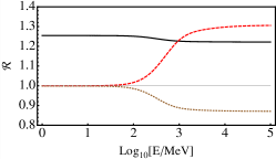
Figure 1: Variation of $\mathcal{R}(E_{\nu})$ with the neutrino/antineutrino energy $E_{\nu}$. The black solid line corresponds to $\eta=0.12$, while in the red dashed and brown dotted lines $\eta=0$. The red dashed line represents the effect of a relatively higher axial mass $M_{A}=1.2$ GeV in the numerator of Eq.5.

Observable Spectra in Ultra-pure Scintillators:

Let us consider an intense beam of neutrinos produced from pion decay at rest according to the usual decay chains $\pi^{+}\to\mu^{+}+\nu_{\mu}\to e^{+}+\nu_{e}+\bar{\nu}_{\mu}+\nu_{\mu}$. The energy spectra of these neutrinos are very well-known and include a monochromatic line for the muonic neutrinos at $(m_{\pi}^{2}-m_{\mu}^{2})/2m_{\pi}=29.8$ MeV and two continuous spectra with energy between $0<E_{\nu}<(m_{\mu}^{2}-m_{e}^{2})/2m_{\mu}=52.8$ MeV. We assume $N_{\pi^{+}}=4.9\times 10^{22}\ \text{pions}/\rm{yr}$ and thus, the same number of $\nu_{e}$, $\nu_{\mu}$ and $\bar{\nu}_{\mu}$. Such a pion production rate can be provided, for example, by a cyclotron with $800$ MeV kinetic energy of protons and with a peak power of $1$ MW daedalus .

We calculate the NC interactions of these $\nu_{e}$, $\nu_{\mu}$ and $\bar{\nu}_{\mu}$ with the protons of a ultra-pure scintillation detector of mass 1 kton located at a distance of 100 meters and with the low energy performances as of Borexino detector BorexPRL . The expected distribution of the elastic scattering events, $\nu(\bar{\nu})+p\to\nu(\bar{\nu})+p$, in the kinetic energy of the final state proton $T_{p}\equiv E^{\prime}_{p}-m_{p}$ can be written as

$$\frac{dN}{dT_{p}}=N_{p}\int_{E_{\mbox{\tiny min}}}\!\!\!\!\!\!\!\!\!dE_{\nu}\left[\frac{d\sigma_{\nu}}{dT_{p}}(E_{\nu},T_{p})\ \Phi_{\nu}(E_{\nu})+(\nu\to\bar{\nu})\right]$$ (6)

where $N_{p}$ is the number of protons in the scintillator, $\sigma_{\nu,\bar{\nu}}$ are the cross sections and $\Phi_{\nu}$ and $\Phi_{\bar{\nu}}$ are the total neutrino and antineutrino fluences (i.e., time integrated fluxes) differential in the neutrino energy $E_{\nu}$. We assume the chemical composition of Borexino, $C_{9}H_{12}$; thus the number of protons in $1$ kton is $N_{p}=6.02\times 10^{31}$ (this increases only by 20% for the composition of LENA, $C_{6}H_{5}C_{n}H_{2n+1}$ with $n=12$ lena ).

The proton kinetic energy $T_{p}$ and the minimum energy of the neutrino in the initial state are related as:

$$E_{\mbox{\tiny min}}=\frac{1}{2}\left[T_{p}+\sqrt{(2m_{p}+T_{p})T_{p}}\right].$$ (7)

The proton kinetic energy has to be converted into an ‘equivalent’ detectable electron energy $E_{d}$, the part of $T_{p}$ that goes into scintillation light. This can be measured and parameterized ianni and we adopt this procedure. Alternatively, one can use the empirical Birks’ formula $E_{d}=\int_{0}^{T_{p}}{dE}/(1+k_{\mbox{\tiny B}}\,({dE}/{dx}))$ birks ; leo , where $dE/dx$ is the stopping power of the proton, that depends on the chemical composition of the detector. In our case, the value $k_{\mbox{\tiny B}}\approx 0.011$ cm/MeV is consistent with ianni and agrees with v .

For the purpose of the analysis we use a Gaussian energy resolution $\sigma(E_{d})=50\ \mbox{keV}\sqrt{E_{d}/\mbox{MeV}}$ similar to Borexino BorexPRL . Therefore, the detection energy threshold $E_{d}^{th}=0.25$ MeV of Borexino corresponds to a proton kinetic energy threshold of about $1.3$ MeV. From Eq. (7), we see that we are sensitive to the highest part of the neutrino energy spectra, $E_{\nu}\geq 25$ MeV.

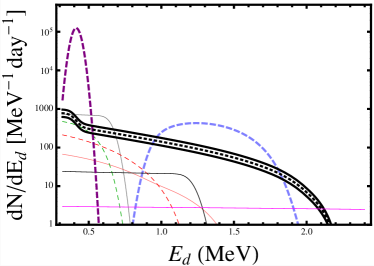
Figure 2: Expected event distribution in the detectable energy $E_{d}$ in 1 kton of scintillator as Borexino. The thick solid and dotted black lines show the event spectrum for neutral current elastic interactions of neutrinos and antineutrinos with protons. The dashed blue line represents the cosmogenic ¹¹C background. The magenta, pink, gray and black solid lines represent ${}^{8}B$, $CNO$, ${}^{7}Be$ and $PeP$ solar neutrino spectrum. The purple, red and green dashed lines represent the backgrounds due to ${}^{210}Po$, ${}^{210}Bi$ and ${}^{85}Kr$, respectively borex .

The differential spectrum $dN/dE_{d}$ expected for 1 year of exposure is shown in Fig. 2. The signal due to NC $\nu p$ interactions is plotted using three black thick lines. They represent the events expected assuming $\eta=0.0,0.12$ (best fit of ahrens ) and 0.25. From Fig. 2 we see that the energy window of interest for the detection of the elastic scattering interactions is $E_{d}=(0.25-2.2)$ MeV. The number of signal events expected in this energy window and for one year of exposure is considerable

strangeness $\eta$	0.00	0.12	0.25
signal events	$0.89\cdot 10^{5}$	$1.14\cdot 10^{5}$	$1.41\cdot 10^{5}$

However, the same energy window will also contain several solar as well as radioactive background events. In particular solar neutrino events from ${}^{7}Be$, $CNO$, $PeP$ and ${}^{8}B$ are not negligible; we expect about $28.6$, $3.0$, $2.1$ and $0.5$ counts per day (cpd) in each 100 tons of scintillator respectively. Moreover, the backgrounds due to radioactive sources as ${}^{210}Po$, ${}^{210}Bi$ and ${}^{85}Kr$, as well as the cosmogenic ${}^{11}C$ have to be considered. We assume that each 100 tons of scintillator yield $10^{3}$ cpd from ${}^{210}Po$, $25$ cpd from both ${}^{85}Kr$ and ${}^{11}C$ as reported in borex . For the ${}^{210}Bi$ we consider $15$ cpd consistent with the present Borexino level aldo . The spectra for these backgrounds are displayed in Fig. 2.

Note incidentally that the Borexino detector is still improving on the background, and in the most recent runs, the ${}^{210}Po$ contaminant has already been halved and the ${}^{85}Kr$ decreased more than three times aldo . The contribution of the ${}^{11}C$ is particularly critical for our purposes, and depends strongly on the depth of the underground site of the detector galbiati . The value of this cosmogenic component is estimated to be 3 times smaller in LENA lena and much less in SNO+ snop . However, in the present study we will adopt the conservative background levels discussed above.

Several meters of rock will moderate the fast neutrons that are subsequently absorbed bas . The irreducible background is due to the neutrinos from the cyclotron. In the region between $(0.25-2.2)$ MeV and for each 100 tons of scintillator, we expect $0.12$ cpd due to elastic scattering on electrons, $0.1$ cpd due $\nu+^{12}\!C\to\nu+p+^{11}\!B$, $0.5$ cpd due to neutron capture following $\nu+^{12}\!C\to\nu+n+^{11}\!C$, $0.5$ cpd due to the protons related to $\nu_{e}+^{12}\!C\to p+e^{-}+^{11}\!C$ Yoshida . All these count rates are at most at the level of ${}^{8}\!B$ background (magenta line in Fig.2). Two of these reactions end with ${}^{11}C$ nuclei. The related increase of the cosmogenic component amounts to $2.5$ cpd per 100 ton. Thus, these irreducible background processes have a minor role and can be safely neglected.

Sensitivity to proton strangeness $\eta$: From Fig. 2, it is evident that background sources can pollute the extraction of the signal. However, following vilante-aldo , we proceed to extract the signal from the total number of observed events, measuring the background events and subtracting them.

If we collect $N=S+B$ events in a time $T$ and $N_{0}=B\cdot T_{0}/T$ events in a time $T_{0}$, when the signal is absent, we expect $S=N-N_{0}\cdot T/T_{0}$ signal events. Since both $N$ and $N_{0}$ are subject to Poissonian fluctuations, the fractional uncertainty caused by the statistical effects is given by:

$$\frac{\Delta S}{S}=\sqrt{\frac{1+\frac{B}{S}\left(1+\frac{T}{T_{0}}\right)}{S}}$$ (8)

If observations are binned in energy, we define $2/\Delta S^{2}\equiv\partial^{2}(\chi^{2})/\partial S^{2}$ using $\chi^{2}=(S_{i}-\bar{S}_{i})^{2}/\Delta S_{i}^{2}$ and $S_{i}=S\rho_{i}$, with $\sum_{i}\rho_{i}=1$. In the minimum of the $\chi^{2}$, $S_{i}=\bar{S}_{i}$, $\frac{\Delta S}{S}=\left\{{\sum_{i=1}^{n}S_{i}/\left[1+\frac{B_{i}}{S_{i}}\left(1+\frac{T}{T_{0}}\right)\right]}\right\}^{-1/2}$. This is smaller than Eq. (8) where we set $S=\sum_{i}S_{i}$ and $B=\sum_{i}B_{i}$, unless the signal and the background have the same shape. For constant background-signal ratio, $B_{i}/S_{i}=$constant, both the results coincide.

From Fig. 2 it is evident that there are two comparatively clean energy windows to extract the signal, one between $(0.65-1.1)$ MeV and another between $(1.73-2.2)$ MeV respectively. Using $T=T_{0}=$1 year, we expect $S_{1}=28900$ and $B_{1}=37200$ events from the first energy window and $S_{2}=1900$ and $B_{2}=2400$ events from the latter one. Since we have $B_{1}/S_{1}\simeq B_{2}/S_{2}$ we can use Eq. (8) obtaining $\Delta S/S=1.1$ %, dominated by the data in the first energy window. If we consider that for a typical pulsed signal daedalus , $T_{0}$ is 4 times larger than $T=1$, the error decreases to $\Delta S/S=0.9$%; a similar improvement is obtained if we measure the background over the range $0.65<E_{d}<2.5$ MeV, increasing the statistic and thus reducing its error.

The NC cross section $\sigma$ at low energy (and therefore the signal event rate $S$) is dominated by the axial form factor, scaling as $(1+\eta)^{2}$, as is clear from Eq. (3). So we can relate the signal sensitivity to the one on $\eta$ through $\delta S=\Delta\sigma/\sigma=2\Delta\eta/(1+\eta)$. This means that the sensitivity $\Delta S/S=1.1$% on the NC signal implies that proton strangeness can be measured with an absolute error of $\Delta\eta=6\cdot 10^{-3}$ for $\eta=0.12$ (similar in size to the heavy quark corrections bass ) i.e., a $5\%$ fractional uncertainty. For all values of $\eta$ in the allowed experimental range, the error is more than 10 times smaller than Eq. (4).

Finally, we show how to attain the same sensitivity with different experimental parameters. Let us write the uncertainty in $\eta$ as follows,

$$\Delta\eta=\frac{1+\eta}{2}\sqrt{\frac{1+\frac{1}{\varphi}\,\frac{B}{S}\left(1+\tau\,\frac{T}{T_{0}}\right)}{\varepsilon\,\varphi\,S}}$$ (9)

Here $\varepsilon=(M^{\prime}/M)(T^{\prime}/T)$ rescales the exposure, proportional to the mass $M^{\prime}$ and to the time of data taking $T^{\prime}$; $\tau=(T^{\prime}/T_{0}^{\prime})/(T/T_{0})$ rescales the fraction of data taking time that includes the signal; $\varphi=(P^{\prime}/P)(D/D^{\prime})^{2}$ rescales the flux, accounting for the new power $P^{\prime}$ and the new distance $D^{\prime}$. Let us adopt the operational parameters of daedalus , i.e., assume a distance from the cyclotron of $D^{\prime}=700$ m, a power increased by a factor of 5 and $T^{\prime}=T_{0}^{\prime}/4=1$ year. The flux (and the signal) decreases by one order of magnitude, for it increases with the power but decreases as the distance squared. In order to compensate for this, we need a larger exposure. E.g., with a mass of 50 kton as in the LENA proposal lena we obtain again $\Delta S/S=1.1$ % after 1 year. Note that the selection of the optimal distance between source and detector will require to minimize the beam related backgrounds.

Summary:

In this work, we explored the possibility to study proton strangeness using low energy neutrinos. We discussed the potential of exploiting a synergy between artificial neutrino beams from pion decay and ultra-pure scintillating detectors. Incidentally, such complex will allow us to quantify precisely the response of underground neutrino detectors, to search for sterile neutrinos and to investigate many more issues.

We showed that, by using reasonable assumptions on the experimental parameters, it is possible to identify two energy windows that allow to measure many tens of thousand of signal events. They imply a statistical error on proton strangeness one order of magnitude smaller than obtained by BNL 734, Eq. (4). It is important to emphasize that the signal we discussed should be collected above 0.6 MeV, and thus, it does not require the extreme low energy threshold reached by Borexino detector.

- (1) S. Weinberg, Phys. Rev. D 5 (1972) 1412.
- (2) J.C Collins et al. Phys. Rev. D 18 (1978) 242. R.N. Mohapatra, G. Senjanovic, Phys. Rev. D 19 (1979) 2165. L. Wolfenstein, Phys. Rev. D 19 (1979) 3450.
- (3) L.A. Ahrens et al. [BNL 734] Phys. Rev. D 35 (1987) 785.
- (4) R. Tayloe, Nucl.Phys.B (Proc. Suppl.) 105 (2002) 62.
- (5) A.A. Aguilar-Arevalo et al. [MiniBooNE] Phys. Rev. D 82 (2010) 092005.
- (6) J. F. Beacom et al. Phys. Rev. D 66 (2002) 033001.
- (7) J. Ellis and M. Karliner, Phys. Lett. B 341 (1995) 397.
- (8) J. Ashman et al. [EMC], Nucl. Phys. B 328 (1989) 1.
- (9) A.V. Efremov and O.V. Teryaev, JINR Report E2-88- 287, Dubna (1988); G. Altarelli and G.G. Ross, Phys. Lett. B 212 (1988) 391.
- (10) W. M. Alberico et al. Phys. Rept. 358 (2002) 227.
- (11) D. de Florian et al. Phys. Rev. Lett. 101 (2008) 072001.
- (12) F.J. Federspiel [LSND], Proc. Lake Louise 1992, p. 330.
- (13) G.T. Garvey, W.C. Louis, D.H. White. Phys. Rev. C 48 (1993) 761.
- (14) C. Arpesella et al. [Borexino], Phys. Rev. Lett. 101 (2008) 091302.
- (15) J. Alonso et al., arXiv:1006.0260.
- (16) A. Bungau et al. [DAEALUS], arXiv:1205.5528.
- (17) M. Sajjad Athar et al. Nucl. Phys. A 764 (2006) 551.
- (18) B. Bodmann et al. [KARMEN], Phys. Lett. B 267 (1991) 321.
- (19) S.D. Bass et al. Phys. Rev. D 66 (2002) 031901.
- (20) S.D. Bass, Rev. Mod. Phys. 77 (2005) 1257.
- (21) http://theory.lngs.infn.it/astroparticle/sn.html
- (22) M. Wurm et al. [LENA], Astropart. Phys. 35 (2012) 685.
- (23) A. Ianni, Proc. of the HASE 2011 workshop, Hamburg 2011, ed. A. Mirizzi et al., Verlag DESY and priv. comm.
- (24) J. B. Birks, Proc. of the Phys. Soc. A 64 (1951) 874.
- (25) W. R. Leo, Techniques for Nuclear and Particle Physics Experiments (Springer-Verlag, Berlin, 1994).
- (26) V.I. Tretyak, Astropart. Phys. 33 (2010) 40.
- (27) G. Bellini et al. [Borexino], Phys. Rev. Lett. 107 (2011) 141302 and Phys. Rev. Lett. 108 (2012) 051302.
- (28) D. Franco, talk given at NOW 2012, available at http://www.ba.infn.it/ now/.
- (29) C. Galbiati et al., Phys. Rev. C 71 (2005) 055805.
- (30) C. Kraus et al. [SNO+], Prog. Part. Nucl. Phys. 64 (2010) 273.
- (31) J.-L. Basdevant, J. Rich, M. Spiro, Fundamentals in Nuclear Physics, (Springer, New York, 2005).
- (32) T. Yoshida et al. Astr. J., 686 (2008) 448.
- (33) A. Ianni et al. Phys. Lett. B 627 (2005) 38.