Interior penalty discontinuous Galerkin method on very general polygonal and polyhedral meshes
Abstract
This paper focuses on interior penalty discontinuous Galerkin methods for second order elliptic equations on very general polygonal or polyhedral meshes. The mesh can be composed of any polygons or polyhedra which satisfies certain shape regularity conditions characterized in a recent paper by two of the authors in [17]. Such general meshes have important application in computational sciences. The usual conforming finite element methods on such meshes are either very complicated or impossible to implement in practical computation. However, the interior penalty discontinuous Galerkin method provides a simple and effective alternative approach which is efficient and robust. This article provides a mathematical foundation for the use of interior penalty discontinuous Galerkin methods in general meshes.
keywords:
discontinuous Galerkin, finite element, interior penalty, second-order elliptic equations, hybrid mesh.AMS:
65N15, 65N30.1 Introduction
Most finite element methods are constructed on triangular and quadrilateral meshes, or on tetrahedral, hexahedral, prismatic, and pyramidal meshes. To extend the idea of the finite element method into meshes employing general polygonal and polyhedral elements, one immediately faces the problem of choosing suitable discrete spaces on general polygons and polyhedrons. This issue has rarely been addressed in the past, partly because it can usually be circumvented by dividing the polygon or polyhedron into sub-elements using only one or two basic shapes. However, allowing the use of general polygonal and polyhedral elements does provide more flexibility, especially for complex geometries or problems with certain physical constraints. One of such example is the modeling of composite microstructures in material sciences. A well-known solution to this problem is the Voronoi cell finite element method [8, 9, 10, 13], in which the mesh is composed of polygons or polyhedrons representing the grained microstructure of the given material. The main difficulty of constructing conforming finite element methods on Voronoi meshes is that, the finite element space has to be carefully chosen so that it is continuous along interfaces. Although the constructions on triangles, quadrilaterals, or three-dimensional simplexes are straight forward, it is not easy for general polygons and polyhedrons. Probably the only practically used solution is the rational polynomial interpolants proposed by Wachspress [16], in which rational basis functions are defined using distances from several “nodes”. An important constraint in the construction of the Wachspress basis is that, the rational basis functions need to be piecewise linear along the boundary of every element, in order to ensure conformity of the finite element space. This not only limits the approximation order of the entire Wachspress finite element space, but also complicates the construction. The Wachspress element has gained a renewed interest recently [6, 7, 14]. However, as we have pointed out above, its construction is complicated and usually requires the aid of computational algebraic systems such as Maple.
Another practically important issue is to define finite element methods on hybrid meshes. Hybrid meshes are frequently used nowadays. It can handle complicated geometries, and can sometimes reduce the total number of unknowns. Another possible reason for using the hybrid mesh is that, some engineers argue that in three-dimensions, a hexahedral mesh yields more accurate solution than a tetrahedral mesh for the same geometry [18, 19], as partly verified by numerical experiments. However, pure hexahedral meshes lack the ability of handling complicated geometries. Hence a hybrid mesh becomes a welcomed compromise between accuracy and flexibility. For conforming finite element methods based on hybrid meshes, continuity requirements on interfaces must be satisfied. Such a coupling is straight-forward for the -conforming finite elements on a triangular-quadrilateral hybrid mesh. However, for three-dimensional meshes, high order finite elements, or other complicated finite element spaces, it usually requires special treatments.
An alternative solution, that can address both issues mentioned above, is to use the weak Galerkin method proposed in [17]. The weak Galerkin method uses discontinuous piecewise polynomials inside each element and on the interfaces to approximate the variational solution. In [17], the authors have proved optimal convergence of the weak Galerkin method for the mixed formulation of second order elliptic equations on very general polygonal and polyhedral meshes. Most of the existing error analysis of finite element methods assume triangular, quadrilateral, or some commonly-seen three-dimensional meshes. To our knowledge, it is the first time that optimal convergence for the finite element solutions has been rigorously proved in [17] for general meshes of arbitrary polygons and polyhedrons.
The discontinuous Galerkin method imposes the interface continuity weakly, and is known to be able to handle non-conformal, hybrid meshes as well as a variety of basis functions. There have been many research works in this direction, for example, nodal discontinuous Galerkin methods [3, 5, 12] for hyperbolic conservation laws. However, we would like to point out that so far there has been no theoretical analysis on the convergence rate of discontinuous Galerkin method, on very general polygonal or polyhedral meshes yet. Motivated by the work in [17], here we would like to fill the gap. The objective of this paper is to establish the theoretical analysis of the interior penalty discontinuous Galerkin method [2] for elliptic equations on very general meshes and discrete spaces.
The paper is organized as follows. In Section 2, we briefly describe the interior penalty discontinuous Galerkin method in an abstract setting. In Section 3, several assumptions on the discrete spaces are listed, which form a minimum requirement for the well-posedness and the approximation property of the discrete formulation. Abstract error estimations are given. In Section 4, we discuss choices of meshes and discrete spaces that satisfy the assumptions given in Section 3. Finally, numerical results are presented in Section 5.
2 The model problem and the interior penalty method
Consider the model problem
| (1) |
where is a closed domain with Lipschitz continuous boundary, and .
For any subdomain with Lipschitz continuous boundary, we use the standard definition of Sobolev spaces with (e.g., see [1, 4] for details). The associated inner product, norm, and seminorms in are denoted by , , and , respectively. When , coincides with the space of square integrable functions . In this case, the subscript is suppressed from the notation of norm, semi-norm, and inner products. Furthermore, the subscript is also suppressed when . Finally, all above notations can easily be extended to any . For the inner product on , we usually denote it as in stead of , as it can be replaced by the duality pair when needed.
For simplicity, we assume that satisfy certain conditions such that Equation (1) has at least regularity with , that is, the solution to Equation (1) satisfies and
| (2) |
This assumption is standard in the practice of interior penalty discontinuous Galerkin methods, as it ensures that the exact solution also satisfies the discontinuous Galerkin formulation, and thus the a priori error estimation can be easily derived in a Lax-Milgram framework. However, such a regularity assumption is not necessary in the practice of interior penalty methods. A well-known technique, which was first proposed by Gudi [11], is to use a posteriori error estimation to derive an a priori error estimation for the interior penalty method, with only minimum regularity requirement . We believe that the same technique applies for the general polygonal and polyhedral meshes, as long as a working a posteriori error estimation is available. However, here we choose to completely skip this issue, as it is not the main purpose of this paper.
Assume that for all set discussed in this paper, including itself, the unit outward normal vector is defined almost everywhere on . Note this is true for all polygonal and polyhedral elements with Lipschitz continuous boundaries. Since the exact solution with , it is clear that for any smooth function defined on ,
where is the -inner product in and is the -inner product in
Let be a partition of the domain into non-overlapping subdomains/elements, each with Lipschitz continuous boundary. Here denotes the characteristic size of the partition, which will be defined in details later. The interior interfaces are denoted by , where , . Boundary segments are similarly denoted by , where . Denote by the set of all interior interfaces and boundary segments in , and by the set of all interior interfaces. For every , let be the area/volume of , and for every , let be its length/area. Denote the diameter of and the diameter of . Clearly, when , we have . Finally, define to be the characteristic mesh size.
Notice that defined above is a very general mesh/partition on , as we do not specify the shape and conformal property of . The interior penalty discontinuous Galerkin (IPDG) method can be extended to such a general mesh, without any modification of the formulation. However, to ensure its approximation rate, certain conditions must be imposed on and the discrete function spaces. In this paper, we are interested in discussing the minimum requirements of such conditions. First, we shall give the formulation of the interior penalty discontinuous Galerkin method.
Let be a finite dimensional space of smooth functions defined on . Define
and
For any internal interface , let and be the unit outward normal vectors on , associated with and , respectively. For , define the average and jump on by
On any boundary segment , the above definitions of average and jump need to be modified:
where is the unit outward normal vector on with respect to .
Define a bilinear form on by
where and . when , the bilinear form is symmetric. The constant is usually required to be large enough, but still independent of the mesh size , in order to guarantee the well-posedness of the discontinuous Galerkin formulation. Details will be given later.
It is clear that the exact solution to Equation (1) satisfies
| (3) |
as vanishes on all . Hence the following interior penalty discontinuous Galerkin formulation is consistent with Equation (1): find satisfying
| (4) |
Finally, we would like to point out that the formulation (4) is computable, as long as each finite dimensional space has a clearly defined and computable basis.
3 Abstract theory
Define a norm on as following:
| (5) |
By the Poincaré inequality, is obviously a well-posed norm on .
Next, we give a set of assumptions, which form the minimum requirements guaranteeing the well-posedness and the approximation properties of the interior penalty discontinuous Galerkin method.
-
I1
(The trace inequality) There exists a positive constant such that for all and , we have
(6) -
I2
(The inverse inequality) There exists a positive constant such that for all , and where , we have
(7) -
I3
(The approximability) There exist positive constants and such that for all , we have
(8)
The abstract theory of the interior penalty discontinuous Galerkin method can be entirely based on Assumptions I1-I3.
Lemma 1.
Assume I1-I2 hold. The bilinear form is bounded in , with respect to the norm . Indeed,
Furthermore, denote . Then for any constant and , the bilinear form is coercive on . That is,
Proof.
The boundedness of follows immediately from the Schwarz inequality. Here we only prove the coercivity. First, notice that for all , by assumptions I1-I2 and the fact that for all ,
Then, by the Schwarz inequality, the Young’s inequality and assumptions I1-I2, we have
where is chosen to be for any given constant . Clearly, for such an , we have and
Combine the above and let , we have
∎
Lemma 1 guarantees the existence and uniqueness of the solution to Equation (4). In the rest of this paper, we shall always assume . Let and be the solution to equations (1) and (4), respectively. By subtracting (3) from (1), one gets the standard orthogonality property of the error,
Then clearly, for all ,
Then, using the triangle inequality,
Combine this with assumption I3, we get the following abstract error estimation:
Theorem 2.
Finally, we derive the error estimation by using the standard duality argument. Let , that is, the bilinear form is symmetric. Consider the following problem
Here again, we assume that the domain satisfies certain condition such that has regularity, with . Let be an approximation to such that they satisfy Assumption I3. Clearly
This gives the following theorem
4 Requirements on meshes and discrete spaces
On triangular or quadrilateral meshes, the usual tool for proving assumptions I1-I3 is to use a scaling argument built on affine transformations. However, on general polygons and polyhedrons, it is not clear how to define such affine transformations. The assumptions I1-I3 were first validated in [17] for general polygonal and polyhedral meshes that satisfy a set of conditions introduced in [17]. Such conditions can be stated as follows.
All the elements of are assumed to be closed and simply connected polygons or polyhedrons. We make the following shape regularity assumptions for the partition .
-
A1:
Assume that there exist two positive constants and such that for every element and , we have
(9) -
A2:
Assume that there exists a positive constant such that for every element and , we have
(10) -
A3:
Assume that for every and , there exists a pyramid contained in such that its base is identical with , its apex is , and its height is proportional to with a proportionality constant bounded away from a fixed positive number from below. In other words, the height of the pyramid is given by such that The pyramid is also assumed to stand up above the base in the sense that the angle between the vector for any , and the outward normal direction of is strictly acute by falling into an interval with .
-
A4:
Assume that each has a circumscribed simplex that is shape regular and has a diameter proportional to the diameter of ; i.e., with a constant independent of Furthermore, assume that each circumscribed simplex intersects with only a fixed and small number of such simplexes for all other elements
Under the above assumptions, the following results have been proved in [17]:
Lemma 4.
(The trace inequality). Assume A1-A3 hold on a polygonal or polyhedral mesh. Then I1 is true.
Lemma 5.
(The inverse Inequality). Assume A1-A4 hold on a polygonal or polyhedral mesh and each is the space of polynomials with degree less than or equal to . Then I2 is true with depending on , but not on or .
Lemma 6.
Assume A1-A4 hold on a polygonal or polyhedral mesh and each is the space of polynomials with degree less than or equal to . Let be the projection onto . Then for all and ,
It is not hard to see that I3 follows immediately from Lemma 6. Indeed, notice that as long as I1 and I2 are true and with , we have
where . Next, notice that by A2, I1 and Lemma 6,
Combine the above, we have
Lemma 7.
(The aproximability) Assume A1-A4 hold on a polygonal or polyhedral mesh and each is the space of polynomials with degree less than or equal to . Then for all and , there exists a constant independent of such that
Here is added so that is well-defined.
5 Numerical Examples
Finally, we present numerical results that support the theoretical analysis of this paper. We fix the coefficients and , since the purpose of the numerical experiments is to examine the accuracy of the interior penalty discontinuous Galerkin method on arbitrary polygonal meshes, not for different coefficients. Consider the Poisson’s equation on with the exact solution . Clearly on . For simplicity of the notation, we denote
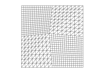
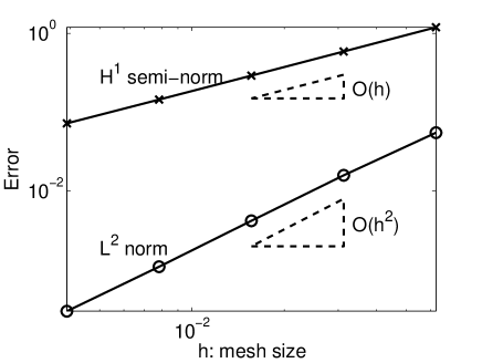
The first test is performed on a non-conformal triangular-quadrilateral hybrid mesh. The initial mesh and the mesh after one uniform refinement are given in Figure 1. A sequence of uniform refinements are then applied to generate a set of nested meshes. Notice that the meshes are non-conformal and there are hanging nodes. However, the interior penalty discontinuous Galerkin method can deal with such meshes without special treatments. We solve the Poisson equation using the interior penalty discontinuous Galerkin formulation (4) on these meshes, where the local discrete spaces are taken to be polynomials on each , no matter whether is a triangle or quadrilateral. The semi-norm and the norm of the errors are reported in Table 1 and Figure 2. These errors are computed using a 5th order Gaussian quadrature on triangles. For quadrilateral elements, the errors can be conveniently computed by dividing the quadrilateral into two triangles and then applying the Gaussian quadrature. Our results show that the semi-norm has an approximate order of , while the norm has an approximate order of , as predicted by the theoretical analysis.

| , | ||||||
|---|---|---|---|---|---|---|
| 1.2006 | 0.5904 | 0.2917 | 0.1452 | 0.0725 | 1.0124 | |
| 0.0551 | 0.0159 | 0.0042 | 0.0011 | 0.0003 | 1.9270 |
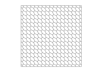
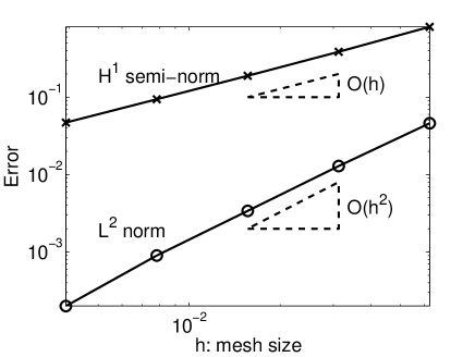
In the second test, we consider a hybrid mesh containing mainly hexagons, but with a few quadrilaterals and pentagons. Indeed, it is derived by taking the dual mesh of a simple triangular mesh. In Figure 3, the initial triangular mesh and its dual mesh are shown. By refining the triangular mesh and computing its dual mesh, we get a sequence of hexagon hybrid meshes. Again, we solve the interior penalty discontinuous Galerkin formulation (4) on these hexagon hybrid meshes, with the local discrete spaces of polynomials. The semi-norm and the norm of the errors are reported in Table 2 and Figure 4. Optimal convergence rates are achieved.

| , | ||||||
|---|---|---|---|---|---|---|
| 0.8139 | 0.3868 | 0.1894 | 0.0941 | 0.0470 | 1.0270 | |
| 0.0461 | 0.0129 | 0.0034 | 0.0009 | 0.0002 | 1.9393 |
References
- [1] R. Adams and J. Fournier, Sobolev Spaces, Academic press, 2003.
- [2] D.N. Arnold, F. Brezzi, B. Cockburn and L.D. Marini, Unified analysis of discontinuous Galerkin methods for elliptic problems, SIAM J. Numer. Anal. 39 (2002), pp. 1749–1779.
- [3] M. Bergot, G. Cohen and M. Duruflé, Higher-order finite elements for hybrid meshes using new nodal pyramidal elements, J. Sci. Comput. 42 (2010), pp. 345–381.
- [4] P.G. Ciarlet, The Finite Element Method for Elliptic Problems, North-Holland, New York, 1978.
- [5] G.C. Cohen, Higher-Order Numerical Methods for Transient Wave Equations, Springer, Berlin, 2000.
- [6] G. Dasgupta, Interpolation within convex polygons: Wachspress’ shape functions, Hournal of Aerospace Engineering, 16 (2003), pp. 1-8.
- [7] G. Dasgupta, Integration within polygonal finite elements, Journal of Aerospace Engineering, 16 (2003), pp. 9-18.
- [8] S. Ghosh and R.L. Mallett, Voronoi cell finite elements, Computers & Structures, 50 (1994), pp. 33–46.
- [9] S. Ghosh and S. Moorthy, Elastic-plastic analysis of arbitrary heterogeneous materials with the Voronoi cell finite-element method, Comput. Methods Appl. Mech. Engrg., 121 (1995), pp. 373–409.
- [10] S. Ghosh and S. Moorthy, Three dimensional Voronoi cell finite element model for microstructures with ellipsoidal heterogeneties, Computational Mechanics, 34 (2004), pp. 510–531.
- [11] T. Gudi, A new error analysis for discontinuous finite element methods for linear elliptic problems, Math. Comp., 79 (2010), pp. 2169–2189.
- [12] J.S. Hesthaven and C.H. Teng, Stable spectral methods on tetrahedral elements, SIAM J. Numer. Anal., 21 (2000), pp. 2352–2380.
- [13] S. Moorthy and S. Ghosh, A Voronoi cell finite element model for partical cracking in elastic-plastic composite materials, Comput. Methods Appl. Mech. Engrg., 151 (1998), pp. 377–400.
- [14] N. Sukumar and E.A. Malsch, Recent advances in the construction of polygonal finite element interpolants, Arch. Comput. Meth. Engrg., 13 (2006), pp. 129–163.
- [15] S.C. Tadepalli, A. Erdemir and P.R. Cavanagh, Comparison of hexahedral and tetrahedral elements in finite element analysis of the foot and footwear, J Biomech., 44 (2011), pp. 2337–2343.
- [16] E.L. Wachspress, A rational finite element basis, Academic Press, New York, 1975.
- [17] J. Wang and X. Ye, A weak Galerkin mixed finite element method for second-order elliptic problems, arXiv:1202.3655v1 [math.NA] 16 Feb 2012.
- [18] S. Yamakawa and K. Shimada, Fully-automated hex-dominant mesh generation with directionality control via packing rectangular solid cells, Int. J. Numer. Meth. Engng., 57 (2003), pp. 2099–2129.
- [19] S. Yamakawa and K. Shimada, Converting a tetrahedral mesh to a prism–tetrahedral hybrid mesh for FEM accuracy and efficiency, Int. J. Numer. Meth. Engng., 80 (2009), pp. 74–102.