Profit Maximization over Social Networks

Abstract

Influence maximization is the problem of finding a set of influential users in a social network such that the expected spread of influence under a certain propagation model is maximized. Much of the previous work has neglected the important distinction between social influence and actual product adoption. However, as recognized in the management science literature, an individual who gets influenced by social acquaintances may not necessarily adopt a product (or technology), due, e.g., to monetary concerns. In this work, we distinguish between influence and adoption by explicitly modeling the states of being influenced and of adopting a product. We extend the classical Linear Threshold (LT) model to incorporate prices and valuations, and factor them into users’ decision-making process of adopting a product. We show that the expected profit function under our proposed model maintains submodularity under certain conditions, but no longer exhibits monotonicity, unlike the expected influence spread function. To maximize the expected profit under our extended LT model, we employ an unbudgeted greedy framework to propose three profit maximization algorithms. The results of our detailed experimental study on three real-world datasets demonstrate that of the three algorithms, PAGE, which assigns prices dynamically based on the profit potential of each candidate seed, has the best performance both in the expected profit achieved and in running time.

1 Introduction

The rapidly increasing popularity of online social networking sites such as Facebook, Google+, and Twitter has facilitated immense opportunities for large-scale viral marketing. Viral marketing was first introduced to the data mining community by Domingos and Richardson [7, 20]; it is a cost-effective method to promote a new product (or technology) by giving free or discounted samples to a selected group of influential individuals, in the hope that through the word-of-mouth effects over the social network, a large number of product adoptions will occur.

Motivated by viral marketing, influence maximization (InfMax) has emerged as a fundamental problem concerning the propagation of innovations through social networks. In their seminal paper, Kempe et al. [16] formulated InfMax as a discrete optimization problem: given a directed graph $G=(V,E)$ (representing a social network) with pairwise influence weights on edges, and a positive number $k$, find $k$ individuals or seeds, such that by activating them initially, the expected spread of influence (or spread for short) in the network under a certain propagation model is maximized. Two classical propagation models studied in [16] are the Independent Cascade (IC) and the Linear Threshold (LT) model. In this paper, we focus on the LT model, the details of which are deferred to Sec. 2.

The expected spread of influence of any set $S\subseteq V$, denoted by $h(S)$, is defined as the expected number of activated nodes after the diffusion process starting from $S$ quiesces. Under both IC and LT models, InfMax is NP-hard and the influence function $h$ is monotone and submodular. A set function $f\colon 2^{X}\mbox{$\rightarrow$}\,\mathbb{R}$ is monotone if $f(S)\leq f(T)$ whenever $S\subseteq T\subseteq X$, where $X$ is the ground set. The function $f$ is submodular if $f(S\cup\{x\})-f(S)\geq f(T\cup\{x\})-f(T)$ holds for all $S\subseteq T\subseteq X$ and $x\in X\setminus T$. Submodularity naturally captures the law of diminishing marginal returns, a fundamental principle in microeconomics. With these good properties, approximation guarantees can be provided for InfMax [16].

Although InfMax has been studied extensively, a majority of the previous work has focused on the classical propagation models, namely IC and LT, which do not fully incorporate important monetary aspects in people’s decision-making process of adopting new products. The importance of such aspects is seen in actual scenarios and recognized in the management science literature. As real-world examples, until recently, Apple’s iPhone has seemingly created bigger buzz in social media than any other smartphones. However, its worldwide market share in 2011 fell behind Nokia, Samsung, and LG. This is partly due to the fact that iPhone is pricier both in hardware (if one buys it contract-free and factory-unlocked) and in its monthly rate plans. On the contrary, the HP TouchPad was shown little interest by the tablet market when it was initially priced at $\$499$ ($16$GB). However, it was sold out within a few days after HP dropped the price substantially to $\$99$ ($16$GB) .

In management science, the adoption of a new product is characterized as a two-step process [15]. In the first step, “awareness”, an individual gets exposed to the product and becomes familiar with its features. In the second step, “actual adoption”, a person who is aware of the product will purchase it if her valuation outweighs the price. Product awareness is modeled as being propagated through the word-of-mouth of existing adopters, which is indeed articulated by classical propagation models. However, the actual adoption step is not captured in these classical models and is indeed the gap between these models and that in [15].

In a real marketing scenario, viral or otherwise, products are priced and people have their own valuations for owning them, both of which are critical in making adoption decisions. Precisely, the valuation of a person for a certain product is the maximum money she is willing to pay for it; the valuation for not adopting is defined to be zero [21]. Thus, when a company attempts to maximize its expected profit in a viral marketing campaign, such monetary factors need to be taken into account. However, in InfMax, only influence weights and network structures are considered, and the marketing strategies are restricted to binary decisions: for any node in the network, an InfMax algorithm just decides whether or not it should be seeded.

To address the aforementioned limitations, we propose the problem of profit maximization (ProMax) over social networks, by incorporating both prices and valuations. ProMax is the problem of finding an optimal strategy to maximize the expected total profit earned by the end of an influence diffusion process under a given propagation model. We extend the LT model to propose a new propagation model named the Linear Threshold model with user Valuations (LT-V), which explicitly introduces the states influenced and adopting. Every user will be quoted a price by the company, and an influenced user adopts, i.e., transitions to adopting, only if the price does not exceed her valuation.

As pointed out by Kleinberg and Leighton [17], people typically do not want to reveal their valuations before the price is quoted for reasons of trust. Moreover, for privacy concerns, after a price is quoted, they usually only reveal their decision of adoption (i.e., “yes” or “no”), but do not wish to share information about their true valuations. Thus, following the literature [17, 21], we make the independent private value (IPV) assumption, under which the valuation of each user is drawn independently at random from a certain distribution. Such distributions can be learned by a marketing company from historical sales data. Furthermore, our model assumes users to be price-takers who respond myopically to the prices offered to them, solely based on their privately-held valuations and the price offered.

Since prices and valuations are considered in the optimization, marketing strategies for ProMax require non-binary decisions: for any node in the network, we (i.e., the system) need to decide whether or not to seed it, and what price should be quoted. Given this factor, the objective function to optimize in ProMax, i.e, the expected total profit, is a function of both the seed set and the vector of prices. As we will show in Secs. 3 and 4, since discounting may be necessary for seeds, the profit function is in general non-monotone. Also, as we show, the profit function maintains submodularity for any fixed vector of prices, regardless of the specific forms of valuation distributions.

In light of the above, ProMax is inherently more complex than InfMax, and calls for more sophisticated algorithms for its solution. As the profit function is in the form of the difference between a monotone submodular set function and a linear function, we first design an “unbudgeted” greedy (U-Greedy) framework for seed set selection. In each iteration, it picks the node with the largest expected marginal profit until the total profit starts to decline. We show that for any fixed price vector, U-Greedy provides quality guarantees slightly lower than a $(1-1/e)$-approximation. To obtain complete profit maximization algorithms, we propose to integrate U-Greedy with three pricing strategies, which leads to three algorithms All-OMP (Optimal Myopic Prices), FFS (Free-For-Seeds), and PAGE (Price-Aware GrEedy). The first two are baselines and choose prices in ad hoc ways, while PAGE dynamically determines the optimal price to be offered to each candidate seed in each round of U-Greedy. Our experimental results on three real-world network datasets illustrate that PAGE outperforms All-OMP and FFS in terms of expected profit achieved and running time, and is more robust against various network structures and valuation distributions.

Road-map.

Sec. 2 discusses related work. Sec. 3 describes the LT-V model and defines ProMax. Sec. 4 presents our profit maximization algorithms. We discuss experiments in Sec. 5, and present extensions and conclusions in Sec. 6.

2 Background and Related Work

Domingos and Richardson [7, 20] first posed InfMax as a data mining problem. They modeled the problem using Markov random fields and proposed heuristic solutions. Kempe et al. [16] studied InfMax as a discrete optimization problem, and utilized submodularity of the spread function $h$ to obtain a greedy $(1-1/e)$-approximation algorithm using the results in [19] (see Algorithm 1: Greedy). Greedy starts from an empty set; in each iteration it adds to $S$ the element with the largest marginal gain until $|S|=k$.

The Linear Threshold Model.

We now describe the LT model [16] in detail. In this model, each node $u_{i}$ chooses an activation threshold $\theta_{i}$ uniformly at random from $[0,1]$, representing the minimum weighted fraction of active in-neighbors necessary so as to activate $u_{i}$. Each edge $(u_{i},u_{j})\in E$ is associated with an influence weight $w_{i,j}$; for each $u_{j}\in V$, $\sum_{u_{i}\in\mathrm{N}^{\mathit{in}}(u_{j})}w_{i,j}\leq 1$, where $\mathrm{N}^{\mathit{in}}(u_{i})$ is the set of in-neighbors of $u_{i}$ (i.e., the sum of incoming weights does not exceed $1$). Time proceeds in discrete steps. At time $0$, a seed set $S$ is activated. At any time $t\geq 1$, we activate any inactive $u_{i}$ if the total influence weight from its active in-neighbors reaches or exceeds $\theta_{i}$. Once a node is activated, it stays active. The diffusion process completes when no more nodes can be activated.

Chen et al. [6] showed that it is #P-hard to compute the exact expected spread of any node set in general graphs for the LT model. Thus, a common practice is to estimate the spread using Monte-Carlo (MC) simulations, in which case the approximation ratio of Greedy drops to $1-1/e-\epsilon$, where $\epsilon>0$ depends on the number of MC simulations run [16]. By further exploiting submodularity, [18] proposed the cost-effective lazy forward (CELF) optimization, which improves the running time of Greedy by up to $700$ times.

Recently, Bhagat et al. [2] addressed the difference between product adoption and influence in their LT-C (Linear Threshold with Colors) model. In LT-C, the extent to which a node is influenced by its neighbors depends on two factors: influence weights and the opinions of the neighbors. LT-C also features a “tattle” state for nodes: if an influenced node does not adopt, it may still propagate positive or negative influence to neighbors. However, unlike us, the LT-C model does not consider monetary aspects in product adoption.

Considerable work has been done on pricing in social networks. Hartline et al. [13] studied optimal marketing for digital goods in social networks and proposed the influence-and-exploit (IE) framework. In IE, seeds are offered free samples, and the seller can approach other users in a random sequence, bypassing the network structure. Arthur et al. [1] adopted IE to study a similar problem in which users arrive in a sequence decided by a cascade model (IC). However, in [1], seeds are given as input (with free samples offered), whereas in our case, the choice of the seed set and of the prices are driven by profit maximization. These choices are made by the algorithms. Work in [3, 4] formulated pricing in social networks as simultaneous-move games and studied equilibria of the games, whereas we focus on stochastic propagation models with social influence.

1 $S\leftarrow\emptyset$;

2 for $i=1\rightarrow k$ do

3       $u\leftarrow\operatorname*{arg\,max}_{u_{i}\in V\setminus S}\left[h(S\cup\{u_{i}\})-h(S)\right]$;

4       $S\leftarrow S\cup\{u\}$;

5      

6 Output $S$;

Algorithm 1 Greedy ($G=(V,E)$, $k$, $h$)

3 Linear Threshold Model with User Valuations and Its Properties

In Sec. 3.1, we describe our proposed LT-V model and define the profit maximization problem (ProMax). We then study a restricted case of ProMax and present theoretical results for it in Sec. 3.2. In Sec. 3.3, we establish the submodularity result for general ProMax.

3.1 Model and Problem Definition

In the LT-V model, the social network is modeled as a directed graph $G=(V,E)$, in which each node $u_{i}\in V$ is associated with a valuation $v_{i}\in[0,1]$. Recall that in Sec. 1, we made the IPV assumption under which valuations are drawn independently at random from some continuous probability distribution assumed known to the marketing company. Let $F_{i}(x)=\Pr[v_{i}\leq x]$ be the distribution function of $v_{i}$, and $f_{i}(x)=\frac{\mathrm{d}}{\mathrm{d}x}F_{i}(x)$ be the corresponding density function. The domain of both functions is $[0,1]$ as we assume both prices and valuations are in $[0,1]$. As in the classical LT model, each node $u_{i}$ has an influence threshold $\theta_{i}$ chosen uniformly at random from $[0,1]$. Each edge $(u_{i},u_{j})\in E$ has an influence weight $w_{i,j}\in[0,1]$, such that for each node $u_{j}$, $\sum_{u_{i}\in\mathrm{N}^{\mathit{in}}(u_{j})}w_{i,j}\leq 1$. If $(u_{i},u_{j})\not\in E$, define $w_{i,j}=0$. Following [7, 20], we assume that there is a constant acquisition cost $c_{a}\in[0,1)$ for marketing to each seed (e.g., rebates, or costs of mailing ads and coupons).

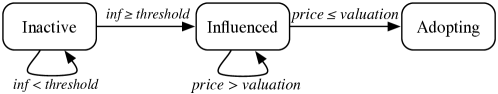
Figure 1: Node states in the LT-V model.

Diffusion Dynamics.

Fig. 1 presents a state diagram for the LT-V model. At any time step, nodes are in one of the three states: inactive, influenced, and adopting. A diffusion under the LT-V model proceeds in discrete time steps. Initially, all nodes are inactive. At time $0$, a seed set $S$ is targeted and becomes influenced. Next, every user $u_{i}$ in the network is offered a price $p_{i}$ by the system. Let $\mathbf{p}=(p_{1},\dotsc,p_{|V|})\in[0,1]^{|V|}$ denote a vector of quoted prices, which remains constant throughout the diffusion. For any $u_{i}\in S$, it gets one chance to adopt (enters adopting state) at step $0$ if $p_{i}\leq v_{i}$; otherwise it stays influenced.

At any time $t\geq 1$, an inactive node $u_{j}$ becomes influenced if the total influence from its adopting in-neighbors reaches its threshold, i.e., $\sum_{u_{i}\in\mathrm{N}^{\mathit{in}}(u_{j})\&\,u_{i}\,\text{adopting}}w_{i,j}\geq\theta_{j}.$ Then, $u_{j}$ will transition to adopting at $t$ if $p_{j}\leq v_{j}$, and will stay influenced otherwise. The model is progressive, meaning that all adopting nodes remain as adopters and no influenced node will ever become inactive. The diffusion ends if no more nodes can change states.

Following [15], we assume that only adopting nodes propagate influence, as adopters can release experience-related product features (e.g., durability, usability), making their recommendations more effective in removing doubts of inactive users. This distinguishes our model from LT-C [2], and in fact, the extensions to the LT model employed in LT-C and in LT-V are orthogonal and address different aspects in propagations of influence and adoption.

Formally, we define $\pi\colon 2^{V}\times[0,1]^{|V|}\to\mathbb{R}$ to be the profit function such that $\pi(S,\mathbf{p})$ is the expected (total) profit earned by the end of a diffusion process under the LT-V model, with $S$ as the seed set and $\mathbf{p}$ as the vector of prices. The problem studied in the paper is as follows.

Definition 1 (Profit maximization (ProMax)).

Given an instance of the LT-V model consisting of a graph $G=(V,E)$ with edge weights, find the optimal pair of a seed set $S$ and a price vector $\mathbf{p}$ that maximizes the expected profit $\pi(S,\mathbf{p})$.

The Virtual Mechanism and Its Truthfulness Guarantee.

Recall that users are assumed to be price-takers making adoption decisions just by comparing the quoted price to their valuation. Thus, it is natural to ask: would an influenced user be better off by acting strategically, i.e., by not deciding solely by comparing her true valuation to the price? In other words, for any pricing strategy used by a company, is it robust against strategic behaviors of users?

In fact, the price-taking procedure in LT-V can be structured as a virtual mechanism that we show is truthful, and hence the dominant strategy for all users is to use true valuation. It is worth emphasizing that the mechanism is virtual since in our model, the company needs not to run it and users will not be asked to declare their valuation.

Definition 2 (The Virtual Mechanism).

An influenced user $u_{i}$ declares some valuation to the company; then $u_{i}$ is sold the product at price $p_{i}$ if $p_{i}$ is no greater than the declared valuation, and not sold otherwise.

Theorem 1 (Truthfulness of the Virtual Mechanism).

The mechanism defined in Definition 2 is truthful. That is, the utility any user $u_{i}$ gets by declaring any number $\hat{v}_{i}\neq v_{i}$ is no greater than that she gets by declaring $v_{i}$ truthfully.

Proof.

Consider the case that the true valuation $v_{i}<p_{i}$. Then, if reporting $v_{i}$ truthfully, $u_{i}$ will not adopt $p_{i}$, and hence her utility is $0$. Suppose that $u_{i}$ reports lower ($\hat{v}_{i}<v_{i}$); she still would not get the product and the utility is still $0$. Suppose otherwise ($u_{i}$ reports higher: $\hat{v}_{i}>v_{i}$). Then, if $\hat{v}_{i}<p_{i}$, the situation is the same, in which $u_{i}$ gets zero utility. If $\hat{v}_{i}\geq p_{i}$, then $u_{i}$ ends up paying $p_{i}$ to adopt and having a negative utility, since $v_{i}-p_{i}<0$.

Then, consider the case that $v_{i}\geq p_{i}$, in which if $u_{i}$ reports truthfully, she will adopt the product by paying $p_{i}$ and enjoy a non-negative utility $v_{i}-p_{i}$. Suppose that $u_{i}$ reports higher ($\hat{v}_{i}>v_{i}$), then she still gets to pay $p_{i}$ and has utility $v_{i}-p_{i}$. Suppose otherwise ($u_{i}$ reports lower: $\hat{v}_{i}<v_{i}$). Then, if $\hat{v}_{i}$ is still no less than $p_{i}$, she still pays $p_{i}$ and has utility $v_{i}-p_{i}$, while if $\hat{v}_{i}$ happens to be lower than $p_{i}$, she will not buy it and has zero utility. And this completes the proof. ∎

3.2 A Restricted Special Case of ProMax under LT-V

To better understand the properties of the LT-V model and the hardness of ProMax, we first study a special case of the problem. We assume the valuation distributions degenerate to an identical single-point, i.e., $\forall u_{i}\in V$, $v_{i}=p$ for some $p\in(0,1]$ with probability $1$. As mentioned in Sec. 1, this is usually not the case; the degeneration assumption here is of theoretical interest only.

For simplicity, we also assume that for every $u_{i}\in S$, the quoted price $p_{i}=0$. Since valuation is the maximum money one is willing to pay for the product, in this case, the optimal pricing strategy is to set $p_{j}=p$, $\forall u_{j}\in V\setminus S$. The situation amounts to restricting the marketing strategy to a binary one: free sample ($p_{i}=0$) for seeds and full price for non-seeds ($p_{j}=p$). Given this pricing strategy, once a node is influenced, it transitions to adopting with probability $1$. Thus, ProMax boils down to a problem to determine a seed set $S$, and the profit function $\pi(S,\mathbf{p})$ reduces to a set function $\hat{\pi}(S)$, since $\mathbf{p}$ is uniquely determined given $S$:

$$\hat{\pi}(S) =p\cdot(h_{L}(S)-|S|)-c_{a}\,|S|$$

$$=p\cdot h_{L}(S)-(p+c_{a})\,|S|,$$ (1)

where $h_{L}(S)$ is the expected number of adopting nodes under the LT-V model by seeding $S$.

In general, the degenerated profit function $\hat{\pi}$ is non-monotone. To see this, let $u$ be any seed that provides a positive profit. Now, clearly $\hat{\pi}(\emptyset)=0<\hat{\pi}(\{u\})$ but $\hat{\pi}(V)\leq 0<\hat{\pi}(\{u\})$, as giving free samples to the whole network will result in a loss of $c_{a}\,|V|$ on account of seeding expenses. Since $\hat{\pi}$ is non-monotone, unlike InfMax, it is natural to not use a budget $k$ for the number of seeds, but instead ask for a seed set of any size that results in the maximum expected profit. In other words, the number of seeds to be chosen, $k$, is not preset, but is rather determined by a solution. This restricted case of ProMax is to find $S=\operatorname*{arg\,max}_{T\subset V}\hat{\pi}(T)$, which we show is NP-hard.

Theorem 2.

The Restricted ProMax problem (RPM) is NP-hard for the LT-V model.

Proof.

Given an instance of the NP-hard Minimum Vertex Cover (MVC) problem, we can construct an instance of the ProMax problem, such that an optimal solution to the ProMax problem gives an optimal solution to the MVC problem. Consider an instance of MVC defined by an undirected $n$-node graph $G=(V,E)$; we want to find a set $S$ such that $|S|=k$ and $k$ is the smallest number such that $G$ has a vertex cover (VC) of size $k$.

The corresponding instance of RPM is as follows: first, we direct all edges in $G$ in both directions to obtain a directed graph $G^{\prime}=(V,E^{\prime})$, where $E^{\prime}$ is the set of all directed edges. Then, for each $u_{i}\in V$, set $\theta_{i}=1$; for each $(u_{i},u_{j})\in E$, define $w_{i,j}=1/\mathrm{d}^{\mathit{in}}(u_{j})$, where $\mathrm{d}^{\mathit{in}}(u_{j})$ is the in-degree of $u_{j}$ in $G^{\prime}$. Lastly, set $p=1$ and $c_{a}=0$, in which case $\hat{\pi}(S)=h_{L}(S)-|S|$. Now, we want show that a set $S\subseteq V$ is a minimum vertex cover (MVC) of $G$ if and only if $S=\operatorname*{arg\,max}_{T\subseteq V}\hat{\pi}(T)$.

$(\Longrightarrow)$. If $S$ is a MVC of $G$, then in ProMax we choose $S$ as the seed set, so that $\hat{\pi}(S)=n-|S|$. This is optimal, shown by contradiction. Suppose otherwise, i.e., there exists some $T\subseteq V$, $T\neq S$, such that $\hat{\pi}(T)>\hat{\pi}(S)$. For the case of $|T|\geq|S|$, we have $\hat{\pi}(T)=h_{L}(T)-|T|\leq h_{L}(T)-|S|$. Since $h_{L}(T)\leq n$, $\hat{\pi}(T)\leq h_{L}(T)-|S|\leq n-|S|=\hat{\pi}(S)$, which is a contradiction. For the case of $|T|<|S|$, let $|S|-|T|=\ell$. Thus, $\hat{\pi}(T)=h_{L}(T)-(|S|-\ell)$. Since $T$ is not a VC, $h_{L}(S)=n$, and it is supposed that $\hat{\pi}(T)>\hat{\pi}(S)$, we have $h_{L}(T)=n-j$, for some $j\in[1,\ell)$. Then, from the way in which influence weights and thresholds are set up, we know there are exactly $j$ nodes in $V\setminus T$ that are not activated. Let $J$ be the set containing those $j$ nodes, and consider the set $T^{\prime}=T\cup J$, for which we have $\hat{\pi}(T^{\prime})=n$. From the proof of Theorem 2.7 of [16], $T^{\prime}$ is a VC of $G$. But since $|T^{\prime}|=|T|+j<|S|$, $T^{\prime}$ is a VC with a strictly smaller size than $S$, which gives a contradiction since $S$ is a MVC.

$(\Longleftarrow)$. Suppose that $S=\operatorname*{arg\,max}_{T\subseteq V}\hat{\pi}(T)$, but $S$ is not a VC of $G$ (we will consider MVC later). This implies that there exists at least one edge $e\in E$ such that both endpoints of $e$, denoted by $u_{i}$ and $u_{j}$, are not in $S$. From the way in which influence weights and thresholds are set up in $G^{\prime}$, we know both $u_{i}$ and $u_{j}$ are not activated. Thus, if we add either one of them, say $u_{i}$, into $S$, $h_{L}(S\cup\{u_{i}\})$ is at least $h_{L}(S)+2$, and thus $\hat{\pi}(S\cup\{u_{i}\})-\hat{\pi}(S)>1$, which contradicts with the fact that $S$ optimizes $\hat{\pi}$. Hence, $S$ must be a VC of $G$. Now suppose that in addition $S$ is not a MVC. Then, there must exist some $x\in S$ such that the node-set $S\setminus\{x\}$ is still a VC of $G$; this means that $h_{L}(S\setminus\{x\})=n$, too. Thus, $\hat{\pi}(S\setminus\{x\})=n-|S|+1>\hat{\pi}(S)=n-|S|$, which is a contradiction. Hence, $S$ is indeed a MVC of $G$.

Now we have shown that an optimal solution to the restricted ProMax problem is an optimal solution to the Minimum Vertex Cover problem, and vice versa; this completes the proof.

∎

Observe that both components of $\hat{\pi}$, $h_{L}(S)$ and $-|S|$, are submodular, which leads to the submodularity of $\hat{\pi}$ as it is a non-negative linear combination of two submodular functions. However, unlike for InfMax, the function is non-monotone and we want to find a set $S$ of any size that maximizes $\hat{\pi}(S)$, so the standard Greedy is not applicable here. In [8], Feige et al. gave a randomized local search ($2/5$-approximation) for maximizing general non-monotone submodular functions. This is applicable to $\hat{\pi}$, but have time complexity $\mathrm{O}(|V|^{3}|E|/\epsilon)$, where $(1+\epsilon/|V|^{2})$ is the per-step improvement factor in the search. By contrast, the function $\hat{\pi}$ is the difference between a monotone submodular function and a linear function, we propose a greedy approach (Algorithm 2 U-Greedy) with time complexity $\mathrm{O}(|V|^{2}|E|)$ and a better approximation ratio, which is slightly lower than $1-1/e$. U-Greedy grows the seed set $S$ in a greedy fashion similar to Greedy, and terminates when no node can provide positive marginal gain w.r.t. $S$.

1 $S\leftarrow\emptyset$;

2 while true do

3       $u\leftarrow\operatorname*{arg\,max}_{u_{i}\in V\setminus S}\left[\hat{\pi}(S\cup\{u_{i}\})-\hat{\pi}(S)\right]$;

4       if $\hat{\pi}(S\cup\{u\})-\hat{\pi}(S)>0$ then

5             $S\leftarrow S\cup\{u\}$;

6            

7       else break;

8      

9 Output $S$;

Algorithm 2 U-Greedy ($G=(V,E)$, $\hat{\pi}$)

Theorem 3.

Given an instance of the restricted ProMax problem under the LT-V model consisting of a graph $G=(V,E)$ with edge weights and objective function $\hat{\pi}$, let $S_{g}\subseteq V$ be the seed set returned by Algorithm 2, and $S^{*}\subseteq V$ be the optimal solution. Then,

$$\hat{\pi}(S_{g})\geq(1-1/e)\cdot\hat{\pi}(S^{*})-\Theta(\max\{|S_{g}|,|S^{*}|\}).$$ (2)

Proof.

Case $(i)$. If $|S^{*}|\leq|S_{g}|$, then since $h_{L}$ is monotone and submodular, $h_{L}(S_{g})\geq(1-1/e)\cdot h_{L}(S^{*})$. Thus, by the definition of $\hat{\pi}$, we have

$$\hat{\pi}(S_{g}) =p\cdot h_{L}(S_{g})-(p+c_{a})\,|S_{g}|$$

$$\geq p(1-1/e)\cdot h_{L}(S^{*})-(p+c_{a})\,|S_{g}|$$

$$=(1-1/e)\cdot\hat{\pi}(S^{*})-(p+c_{a})\,|S_{g}|+(1-1/e)(p+c_{a})\,|S^{*}|$$

$$=(1-1/e)\cdot\hat{\pi}(S^{*})-\Theta(S_{g}).$$

Case $(ii)$. If $|S^{*}|>|S_{g}|$, consider a set $S^{\prime}_{g}$ obtained by running U-Greedy until $|S^{\prime}_{g}|=|S^{*}|$. Clearly, from case $(i)$, we have $\hat{\pi}(S^{\prime}_{g})\geq(1-1/e)\cdot\hat{\pi}(S^{*})-\Theta(|S^{\prime}_{g}|)$. Due to the fact that $|S^{*}|=|S^{\prime}_{g}|>|S_{g}|$, and $S_{g}$ is obtained by running U-Greedy until no node can provide positive marginal profit, we have $\hat{\pi}(S_{g})\geq\hat{\pi}(S^{\prime}_{g})\geq(1-1/e)\cdot\hat{\pi}(S^{*})-\Theta(|S^{*}|)$. Combining the above two cases gives Eq. (2). ∎

Theorem 3 indicates that the gap between the U-Greedy solution and a $(1-1/e)$-approximation grows linearly w.r.t. the cardinality of the seed set. Since this cardinality is typically much smaller than the expected spread, U-Greedy can provides quality guarantees for restricted ProMax with objective function $\hat{\pi}$.

3.3 Properties of the LT-V Model in the General Case

Theorem 2 shows that in a restricted setting where exact valuations are known and the optimal pricing strategy is trivial, ProMax is still NP-hard. Now we consider the general ProMax described in Sec. 3.1, and show that for any fixed price vector, the general profit function maintains submodularity (w.r.t. the seed set) regardless of the specific forms of the valuation distributions.

Given a seed set $S$ and a price vector $\mathbf{p}$, let $ap(u_{i}|S,\mathbf{p})$ denote $u_{i}$’s adoption probability, defined as the probability that $u_{i}$ adopts the product by the end of the diffusion started with seed set $S$ and price vector $\mathbf{p}$. Similarly, let $ip(u_{i}|S,\mathbf{p}_{-i})$ denote $u_{i}$’s probability of getting influenced under the same initial conditions, where $\mathbf{p}_{-i}\in[0,1]^{|V|-1}$ is the vector of all prices excluding $p_{i}$. Also, let $\pi^{(i)}(S,\mathbf{p})$ be the expected profit earned from $u_{i}$. By model definition, for any $u_{i}\in V\setminus S$, we have $ap(u_{i}|S,\mathbf{p})=ip(u_{i}|S,\mathbf{p}_{-i})\cdot(1-F_{i}(p_{i}))$ and $\pi^{(i)}(S,\mathbf{p})=p_{i}\cdot ap(u_{i}|S,\mathbf{p})$. If $u_{i}\in S$, $ip(u_{i}|S,\mathbf{p}_{-i})=1$ and $\pi^{(i)}(S,\mathbf{p})=p_{i}\cdot(1-F_{i}(p_{i}))-c_{a}$.

By linearity of expectations, we have $\pi(S,\mathbf{p})=\sum_{u_{i}\in V}\pi^{(i)}(S,\mathbf{p})$. Hence, to analyze the profit function, we just need to focus on the adoption probability, in which the factor $(1-F_{i}(p_{i}))$ does not depend on $S$, but $ip(u_{i}|S,\mathbf{p}_{-i})$ calls for careful analysis, which we will present in the proof of Theorem 4.

Let $\mathbf{v}=(v_{1},\dots,v_{|V|})\in[0,1]^{|V|}$ be a vector of user valuations, corresponding to random samples drawn from the various user valuation distributions. We now have:

Theorem 4 (Submodularity).

Given an instance of the LT-V model, for any fixed vector $\mathbf{p}\in[0,1]^{|V|}$ of prices, the profit function $\pi(S,\mathbf{p})$ is submodular w.r.t. $S$, for an arbitrary vector $\mathbf{v}$ of valuation samples.

The proof of submodularity of the influence spread function $h$ in the classical LT model [16] relies on establishing an equivalence between the LT model and reachability in a family of random graphs generated as follows: for each node $u_{i}\in V$, select at most one of its incoming edges at random, such that $(u_{j},u_{i})$ is selected with probability $w_{j,i}$, and no edge is selected with probability $1-\sum_{u_{j}\in\mathrm{N}^{\mathit{in}}(u_{i})}w_{j,i}$. We will use a similar approach in the proof of Theorem 4.

Proof of Theorem 4.

By linearity of expectation as well as the above analysis on adoption probabilities, $\pi(S,\mathbf{p})=\sum_{u_{i}\in V}\pi^{(i)}(S,\mathbf{p})=\sum_{u_{i}\in S}[p_{i}(1-F_{i}(p_{i}))-c_{a}]+\sum_{u_{i}\not\in S}p_{i}(1-F_{i}(p_{i}))\cdot ip(u_{i}|S,\mathbf{p}_{-i})$. Since the first sum is linear in $S$, it suffices to show that $ip(u_{i}|S,\mathbf{p}_{-i})$ is submodular in $S$, whenever $u_{i}\not\in S$.

To encode random events of the LT-V model using the possible world semantics, we do the following. First, we run a node coloring process on $G$: for each node $u_{i}$, if $p_{i}\leq v_{i}$, color it black; otherwise color it white. Meanwhile, we run a live-edge selection process following the aforementioned protocol [16]. Note that the two processes are orthogonal and independent of each other. Combining the results of both leads to a colored live-edge graph, which we call a possible world $X$. Let $\mathcal{X}$ be the probability space in which each sample point specifies one such possible world $X$.

Next, we define the notion of “black-reachability”. In any possible world $X$, a node $u_{i}$ is black-reachable from a node set $S$ if and only if there exists a black node $s\in S$ such that $u_{i}$ is reachable from $s$ via a path consisting entirely of black nodes, except possibly for $u_{i}$ (even if $u_{i}$ is white, it is still considered black-reachable since here we are interested in the probability of being influenced, not adopting). From the same argument in the proof of Claim 2.6 of [16], on any black-white colored graph, the following two distributions over the sets of nodes are the same: (1) the distribution over sets of influenced nodes obtained by running the LT-V process to completion starting from $S$; (2) the distribution over sets of nodes that are black-reachable from $S$, under the live-edge selection protocol.

Let $I_{X}(u_{i}|S)$ be the indicator set function such that it is $1$ if $u_{i}$ is black-reachable from $S$, and $0$ otherwise. Consider two sets $S$ and $T$ with $S\subseteq T\subseteq V$, and a node $x\in V\setminus T$. Consider some $u_{i}$ that is black-reachable from $T\cup\{x\}$ but not from $T$. This implies (1) $u_{i}$ is not black-reachable from $S$ either (otherwise, $u_{i}$ would also be black-reachable from $T$, which is a contradiction); (2) the source of the path that “black-reaches” $u_{i}$ must be $x$. Hence, $u_{i}$ is black-reachable from $S\cup\{x\}$, but not from $S$, which implies $I_{X}(u_{i}|S\cup\{x\})-I_{X}(u_{i}|S)=1\geq 1=I_{X}(u_{i}|T\cup\{x\})-I_{X}(u_{i}|T)$. Thus, $I_{X}(u_{i}|S)$ is submodular. Since $ip(u_{i}|S,\mathbf{p}_{-i})=\sum_{X\in\mathcal{X}}\Pr[X]\cdot I_{X}(u_{i}|S)$ is a nonnegative linear combination of submodular functions, this completes the proof. ∎

We also remark that in general graphs, given any $S$ and $\mathbf{p}$, it is #P-hard to compute the exact value of $\pi(S,\mathbf{p})$ for the LT-V model, just as in the case of computing the exact expected spread of influence for the LT model. This can be shown using a proof similar to the one for Theorem 1 in [6].

4 Profit Maximization Algorithms

For ProMax, since the expected profit is a function of both the seed set and the vector of prices, a ProMax algorithm should determine both the seed set and an assignment of prices to nodes to optimize the expected profit. Accordingly, it has two components: (1). a seed selection procedure that determines $S$, and (2). a pricing strategy that determines $\mathbf{p}$. Due to acquisition costs and the possible need for seed-discounting (details later), $\pi(S,\mathbf{p})$ is still non-monotone in $S$ and is in the form of the difference between a monotone submodular function and a linear function. Hence, inspired by the restricted ProMax studied in 3.2, we propose to use U-Greedy for seed set selection.

We then propose three pricing strategies and integrate them with U-Greedy to obtain three ProMax algorithms. The first two, All-OMP and FFS, are baselines with simple strategies that set prices of seeds without considering the network structure and influence spread, while the third one, PAGE, computes optimal discounts for candidate seeds based on their “profit potential”. Intuitively, it “rewards” seeds with higher influence spread by giving them a deeper discount to boost their adoption probabilities, and in turn the adoption probabilities of nodes that may be influenced directly or indirectly by such seeds.

Notice that taking valuations into account when modeling the diffusion process of product adoption makes a difference for a marketing company. A pricing strategy that does not consider valuations is limited: either it charges everyone full price (or at best gives full discount to the seeds), or it uses an ad-hoc discount policy which is necessarily suboptimal. By contrast, PAGE makes full use of valuation information to determine the best discounts.

4.1 Two Baseline Algorithms: All-OMP and FFS

Recall that in our model, users in the social network are price-takers who myopically respond to the price offered to them. Thus, given a distribution function $F_{i}$ of valuation $v_{i}$, the optimal myopic price (OMP) [13] can be calculated by:

$$p^{m}_{i}=\operatorname*{arg\,max}_{p\in[0,1]}\;p\cdot(1-F_{i}(p)).$$ (3)

Offering OMP to a single influenced node ensures that the expected profit earned solely from that node is the maximum. This gives our first ProMax algorithm, All-OMP, which offers OMP to all nodes regardless of whether a node is a seed or how influential it is. First, for each $u_{i}\in V$, it calculates $p^{m}_{i}$ using Eq. (3), and populates all OMPs to form the price vector $\mathbf{p}^{m}=(p_{1}^{m},...,p_{|V|}^{m})$. Then, treating $\mathbf{p}^{m}$ fixed, it essentially runs U-Greedy (Algorithm 2) to select the seeds. When the algorithm cannot find a node of which the marginal profit is positive, it stops.

1 $S\leftarrow\emptyset$; $\mathbf{p}^{m}\leftarrow\mathbf{0}$;

2 foreach $u_{i}\in V$ do

3       $\mathbf{p}^{m}[i]\leftarrow p^{m}_{i}=\operatorname*{arg\,max}_{p\in[0,1]}\;p\cdot(1-F_{i}(p))$;

4      

5 while $true$ do

6       $u\leftarrow\operatorname*{arg\,max}_{u_{i}\in V\setminus S}[\pi(S\cup\{u_{i}\},\mathbf{p}^{m})-\pi(S,\mathbf{p}^{m})]$;

7       if $\pi(S\cup\{u\},\mathbf{p}^{m})-\pi(S,\mathbf{p}^{m})>0$ then $S\leftarrow S\cup\{u\}$;

8       else  break;

9      

10 Output $S,\mathbf{p}^{m}$;

Algorithm 3 All-OMP ($G=(V,E)$, $\pi$, $F_{i}(\forall u_{i}\in V)$)

Notice that Eq. (3) overlooks the network structure and ignores the profit potential of seeds. This may lead to the sub-optimality of All-OMP in general. Fig 2 illustrates this with an example.

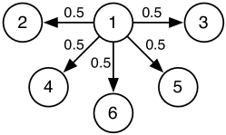
Figure 2: An example graph.

Suppose that all valuations are distributed uniformly in $[0,1]$ and the acquisition cost $c_{a}=0.001$. Hence, $\mathbf{p}^{m}=(1/2,\dotsc,1/2)$. Consider seeding node $1$: it adopts w.p. $0.5$, giving a profit of $0.5+5*0.5^{3}-0.001=1.124$; it does not adopt w.p. $0.5$, resulting in a profit of $-0.001$. Thus, the expected profit $\pi(\{1\},\mathbf{p}^{m})=0.5615$. However, when $p_{1}=3/16$, $\pi(\{1\},\mathbf{p}^{m}_{-1}\oplus(3/16))=0.661$. This shows that for high-influence networks and low acquisition cost, the profit earned by running All-OMP can be improved by seed-discounting, i.e., lowering prices for seeds so as to boost their adoption probabilities and thus better leverage their influence over the network. The intuition is that the profit loss over seeds (stemming from the discount) can potentially be compensated and even surpassed by the profit gain over non-seeds: more seeds may adopt as a result of the discount and the probabilities of non-seeds getting influenced will go up as more seeds adopt.

Generally speaking, there exists a trade-off between the immediate (myopic) profit earned from seeds and the potentially more profit earned from non-seeds. Favoring the latter, we propose our second algorithm FFS (Free-For-Seeds) which gives a full discount to seeds and charges non-seeds the OMP. FFS first calculates $\mathbf{p}^{m}=(p_{1}^{m},...,p_{|V|}^{m})$ using Eq. (3). Then it runs U-Greedy: in each iteration, it adds to $S$ the node which provides the largest marginal profit when a full discount (i.e., price $0$) is given. For all seeds added, their prices remain $0$; the algorithm ends when no node can provide positive marginal profit.

1 $S\leftarrow\emptyset$; $\mathbf{p}^{f}\leftarrow\mathbf{0}$;

2 foreach $u_{i}\in V$ do

3       $\mathbf{p}^{f}[i]\leftarrow p^{m}_{i}=\operatorname*{arg\,max}_{p\in[0,1]}\;p\cdot(1-F_{i}(p))$;

4      

5 while $true$ do

6       $u\leftarrow\operatorname*{arg\,max}_{u_{i}\in V\setminus S}[\pi(S\cup\{u_{i}\},\mathbf{p}^{f}_{-i}\oplus 0)-\pi(S,\mathbf{p}^{f})]$;

7       if $\pi(S\cup\{u\},\mathbf{p}^{f}_{-u}\oplus 0)-\pi(S,\mathbf{p}^{f})>0$ then

8             $S\leftarrow S\cup\{u\}$; $\mathbf{p}^{f}\leftarrow\mathbf{p}^{f}_{-u}\oplus 0$;

9            

10      else  break;

11      

12 Output $S,\mathbf{p}^{f}$;

Algorithm 4 FFS ($G=(V,E)$, $\pi$, $F_{i}(\forall u_{i}\in V)$)

Since FFS has a completely opposite attitude towards seed-discounting compared to All-OMP, intuitively, it should be suitable for high-influence networks and low acquisition costs, but it may be overly aggressive for low-influence networks and high acquisition costs. For example, in Fig 2, the FFS profit by seeding node $1$ is $0.625$, better than the All-OMP profit $0.5615$. But if all influence weights are $0.01$ instead of $0.5$, and $c_{a}=0.01$, All-OMP gives a profit of $0.246$, while FFS gives only $0.0025$.

4.2 The PAGE Algorithm

Both All-OMP and FFS are easy for marketing companies to operate, but they are not balanced and are not robust against different input instances as illustrated above by examples. To achieve more balance, we propose the PAGE (for Price-Aware GrEedy) algorithm (Algorithm 5). PAGE also employs U-Greedy to select seeds. It initializes all seed prices to their OMP values (Step 3). In each round, it calculates the best price for each candidate seed such that its marginal profit (MP) w.r.t. the chosen $S$ and $\mathbf{p}$ is maximized (Step 7); then it picks the node with the largest maximum MP (Step 8). It stops when it cannot find a seed with a positive MP (Step 11). For all non-seed nodes, PAGE still charges OMP. We next explain the details of determining the best price for a candidate seed.

Given a seed set $S$, consider an arbitrary candidate seed $u_{i}\in V\setminus S$, with its price $p_{i}$ to be determined. The marginal profit ($MP$) that $u_{i}$ provides w.r.t. $S$ with $p_{i}$ is $MP(u_{i})=\pi(S\cup\{u_{i}\},\mathbf{p}_{-i}\oplus p_{i})-\pi(S,\mathbf{p}_{-i}\oplus p_{i}^{m})$, where $\mathbf{p}_{-i}$ is fixed. The key task in PAGE is to find $p_{i}$ such that $MP(u_{i})$ is maximized. Since $\pi(S,\mathbf{p}_{-i}\oplus p_{i}^{m})$ does not involve $u_{i}$ and $p_{i}$, it suffices to find $p_{i}$ that maximizes $\pi(S\cup\{u_{i}\},\mathbf{p}_{-i}\oplus p_{i})$.

Seeding $u_{i}$ at a certain price $p_{i}$ results in two possible worlds: world $X_{1}^{(i)}$ with $\Pr[X_{1}^{(i)}]=1-F_{i}(p_{i})$, in which $u_{i}$ adopts, and world $X_{0}^{(i)}$ with $\Pr[X_{0}^{(i)}]=F_{i}(p_{i})$, in which $u_{i}$ does not adopt. In world $X_{1}^{(i)}$, the profit earned from $u_{i}$ is $p_{i}-c_{a}$ and let the expected profit earned from other nodes be $Y_{1}$. Similarly, in world $X_{0}^{(i)}$, the profit from $u_{i}$ is $-c_{a}$ and let the expected profit from other nodes be $Y_{0}$. Notice that $Y_{1}$ depends on the influence of $u_{i}$ but $Y_{0}$ does not. Putting it all together, the quantity of $\pi(S\cup\{u_{i}\},\mathbf{p}_{-i}\oplus p_{i})$ can be expressed as a function of $p_{i}$ as follows:

$$g_{i}(p_{i})=(1-F_{i}(p_{i}))\cdot(p_{i}+Y_{1})+F_{i}(p_{i})\cdot Y_{0}-c_{a}\,.$$ (4)

Similarly to the expected spread of influence in InfMax, the exact values of $Y_{1}$ and $Y_{0}$ cannot be computed in PTIME (due to #P-hardness [6]), but sufficiently accurate estimations can be obtained by Monte Carlo (MC) simulations.

Finding $p_{i}^{*}=\operatorname*{arg\,max}_{p_{i}\in[0,1]}g_{i}(p_{i})$ now depends on the specific form of the distribution function $F_{i}$. We consider two kinds of distributions: the normal distribution, for which $v_{i}\sim\mathcal{N}(\mu,\sigma^{2}),\,\forall u_{i}\in V$, and the uniform distribution, for which $v_{i}\sim\mathcal{U}(0,1),\,\forall u_{i}\in V$. The choice of the normal distribution is supported by evidence from real-world data from Epinions.com (see Sec. 5), and also work in [14]. When sales data are not available, it is common to consider the uniform distribution with support $[0,1]$ to account for our complete lack of knowledge [21, 3].

The Normal Distribution Case.

For normal distribution, assume that $v_{i}\sim\mathcal{N}(\mu,\sigma^{2})$ for some $\mu$ and $\sigma$, then $\forall p_{i}\in[0,1]$,

$$F_{i}(p_{i})=\frac{1}{2}\left[1+\mathrm{erf}\left(\frac{p_{i}-\mu}{\sqrt{2}\sigma}\right)\right],$$

where $\mathrm{erf}(\cdot)$ is the error function, defined as

$$\mathrm{erf}(x)=\frac{2}{\sqrt{\pi}}\int_{0}^{x}e^{-t^{2}}\,\mathrm{d}t.$$

Plugging $F_{i}(\cdot)$ back into Eq. (4), one cannot obtain an analytical solution for $p_{i}^{*}$, as $\mathrm{erf}(x)$ has no closed-form expression. Thus, we turn to numerical methods to approximately find $p_{i}^{*}$. Specifically, we use the golden section search algorithm, a technique that finds the extremum of a unimodal function by iteratively shrinking the interval inside which the extremum is known to exist [9]. In our case, the search algorithm starts with the interval $[0,1]$, and we set the stopping criteria to be that the size of the interval which contains $p_{i}$ is strictly smaller than $10^{-8}$.

The Uniform Distribution Case.

The uniform distribution has easier calculations and analytical solutions. If $v_{i}\sim\mathcal{U}(0,1)$, then $\forall p_{i}\in[0,1]$, $F_{i}(p_{i})=p_{i}$, and plugging it back to Eq. (4) gives

$$g_{i}(p_{i})=-p_{i}^{2}+(1-Y_{1}+Y_{0})\cdot p_{i}+Y_{1}-c_{a}.$$

Hence, the optimal price

$$p_{i}^{*}=\frac{(1+Y_{1}-Y_{0})}{2}.$$

For both normal and uniform distributions, if $p_{i}^{*}>1$ or $p_{i}^{*}<0$, it is normalized back to $1$ or $0$, respectively. Also note that the above solution framework applies to any probability distribution that $v_{i}$ may follow, as long as an analytical or numerical solution can be found for $p_{i}^{*}$.

To conclude this section, steps 5-5 in Algorithm 5 (and also the U-Greedy seed selection procedure in All-OMP and FFS) can be accelerated by the CELF optimization [18], or the more recent CELF++ [11]. The adaptation is straightforward and the details can be found in [18] and [11].

1 $S\leftarrow\emptyset$; $\mathbf{p}\leftarrow\mathbf{0}$;

2 foreach $u_{i}\in V$ do

3       $\mathbf{p}[i]\leftarrow p^{m}_{i}=\operatorname*{arg\,max}_{p\in[0,1]}\;p\cdot(1-F_{i}(p))$;

4      

5 while $true$ do

6       foreach $u_{i}\in V\setminus S$ do

7             Estimate the value of $Y_{0}$ and $Y_{1}$ by MC simulations;

8             $p_{i}^{*}\leftarrow\operatorname*{arg\,max}_{p_{i}\in[0,1]}g_{i}(p_{i})$; normalize if needed;

9            

10       $u\leftarrow\operatorname*{arg\,max}_{u_{i}\in V\setminus S}g_{i}(p_{i}^{*})$;

11       if $\pi(S\cup\{u_{i}\},\mathbf{p}_{-i}\oplus p_{i}^{*})-\pi(S,\mathbf{p}_{-i}\oplus p_{i}^{m})>0$ then

12             $S\leftarrow S\cup\{u_{i}\}$; $\mathbf{p}\leftarrow\mathbf{p}_{-i}\oplus p_{i}^{*}$;

13            

14      else  break;

15      

16 Output $S,\mathbf{p}$;

Algorithm 5 PAGE ($G=(V,E)$, $\pi$, $F_{i}(\forall u_{i}\in V)$)

5 Empirical Evaluations

Table 1: Statistics of Network Data.

Dataset	Epinions	Flixster	NetHEPT
Number of nodes	$11$K	$7.6$K	$15$K
Number of edges	$119$K	$50$K	$62$K
Average out-degree	$10.7$	$6.5$	$4.12$
Maximum out-degree	$1208$	$197$	$64$
#Connected components	$4603$	$761$	$1781$
Largest component size	$5933$	$2861$	$6794$

We conduct experiments on real-world network datasets to evaluate our proposed baselines and the PAGE algorithm. In all these algorithms, a key step is to compute the marginal profit of a candidate seed. As mentioned in Sec. 3, computing the exact expected profit is intractable for the LT-V model. Thus, we estimate the expected profit with Monte Carlo (MC) simulations. Following [16], we run 10,000 simulations for this purpose. This is an expensive step and as for InfMax, it limits the size of networks on which we can run these simulations. For the same reason, the CELF optimization is used in all algorithms as a heuristic. All implementations are in C++ and all experiments were run on a server with $2.50$GHz eight-core Intel Xeon E5420 CPU, $16$GB RAM, and Windows Server 2008 R2.

5.1 Dataset Preparations

Network Data.

We use three network datasets whose statistics are summarized in Table 1. They include: (a) Epinions [20], a who-trust-whom network extracted from review site Epinions.com: an edge $(u_{i},u_{j})$ is present if $u_{j}$ has expressed her trust in $u_{i}$’s reviews; (b) Flixster, a friendship network from social movie site Flixster.com: if $u_{i}$ and $u_{j}$ are friends, we have edges in both directions; (c) NetHEPT (standard for InfMax [16, 5, 6, 12]), a co-authorship network extracted from the High Energy Physics Theory section of arXiv.org: if $u_{i}$ and $u_{j}$ have co-authored papers, we have edges in both directions. The raw data of Epinions and Flixster contain $76$K users, $509$K edges and $1$M users, $28$M edges, respectively. We use the METIS graph partition software to extract a subgraph for both networks, to ensure that MC simulations can finish in a reasonable amount of time.

(a) Weighted Distribution

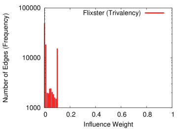
(b) Trivalency

Figure 3: Distribution of influence weights in Flixster

Influence Weights.

We use two methods, Weighted Distribution (WD) and Trivalency (TV), to assign influence weights to edges. For WD, $w_{i,j}=A_{i,j}/N_{j}$, where $A_{i,j}$ is the number of actions $u_{i}$ and $u_{j}$ both perform, and $N_{j}$ is a normalization factor, i.e., the number of actions performed by $u_{j}$, to ensure $\sum_{u_{i}\in\mathrm{N}^{\mathit{in}}(u_{j})}w_{i,j}\leq 1$. In Flixster, $A_{i,j}$ is the number of movies $u_{j}$ rated after $u_{i}$; in NetHEPT, $A_{i,j}$ is the number of papers $u_{i}$ and $u_{j}$ co-authored; in Epinions, since no action data is available, we use $w_{i,j}=1/\mathrm{d}^{\mathit{in}}(u_{j})$ as an approximation. For TV, $w_{i,j}$ is selected uniformly at random from $\{0.001,0.01,0.1\}$, and is normalized to ensure $\sum_{u_{i}\in\mathrm{N}^{\mathit{in}}(u_{j})}w_{i,j}\leq 1$. Fig. 3 illustrates the distribution of weights for Flixster; it shows that influence is higher in WD graphs than in TV graphs.

Valuation Distributions.

As mentioned in Sec. 1, valuations are difficult to obtain directly from users, and we have to estimate the distribution using historical sales data. In an Epinions.com review, a user provides an integer rating from $1$ to $5$, and may optionally report the price she paid in US dollars (see, e.g., http://tinyurl.com/773to53). If a review contains both price and rating, we can combine them to approximately estimate the valuation of that user, as in such systems, ratings are seen as people’s utility for a good, and utility is the difference of valuation and price [21].

We observed that most products have only a limited number ($<100$) of reviews, and thus a single product may not provide enough samples. To circumvent this difficulty, we acquired all reviews for the popular Canon EOS 300D, 350D, and 400D cameras. Given that these cameras followed a sequential release within a short time span (three years), we treated them as having similar monetary values to consumers. After removing reviews without prices reported, we are left with $276$ samples. Next, we transform prices and ratings to obtain estimated valuations as follows:

$$\mathrm{valuation}=\mathrm{price}*(1+\mathrm{rating}\,/\,5).$$

We then normalize the results into $[0,1]$ and fit the data to a normal distribution $\mathcal{N}(\mu,\sigma^{2})$ with $\mu=0.53$ and $\sigma=0.14$ estimated by maximum likelihood estimation (MLE). Fig. 4(a) plots the histogram of the normalized valuations; Fig. 4(b) presents the CDFs of our empirical data and $\mathcal{N}(0.53,0.14^{2})$. To test the goodness of fit, we compute the Kolmogorov-Smirnov (K-S) statistic [10] of the two distributions, which is defined as the maximum difference between the two CDFs; in our case, the K-S statistic is $0.1064$. As can be seen from Fig. 4(b), $\mathcal{N}(0.53,0.14^{2})$ is indeed a good fit for the estimated valuations of the three Canon EOS cameras on Epinions.com.

Since there are no price data to be collected in Flixster and NetHEPT, we use $\mathcal{N}(0.53,0.14^{2})$ in the simulations for all datasets. In addition, for completeness, we also test with the uniform distribution over $[0,1]$, i.e., $\mathcal{U}(0,1)$, as it is commonly assumed in the literature [21, 3].

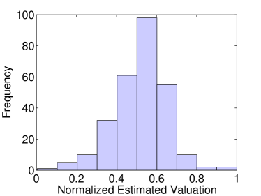
(a) Histogram of valuations

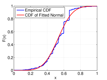
(b) Empirical & normal CDFs

Figure 4: Statistics of Valuations (Epinions.com)

5.2 Experimental Results

We compare PAGE, All-OMP, and FFS in terms of the expected profit achieved, price assignments, and running time. Although all algorithms employ U-Greedy which does not terminate until the marginal profit starts decreasing, for uniformity, we report simulation results up to $100$ seeds.

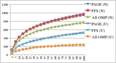
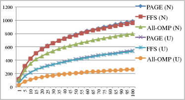
(a) WD with $c_{a}=0.1$	(b) WD with $c_{a}=0.001$
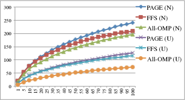
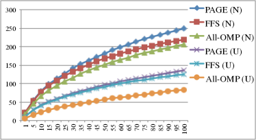
(c) TV with $c_{a}=0.1$	(d) TV with $c_{a}=0.001$

Figure 5: Expected profit achieved (Y-axis) on Epinions graphs w.r.t. $|S|$ (X-axis). (N)/(U) denotes normal/uniform distribution.

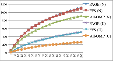
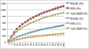
(a) WD with $c_{a}=0.1$	(b) WD with $c_{a}=0.001$
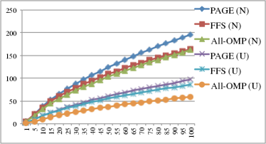
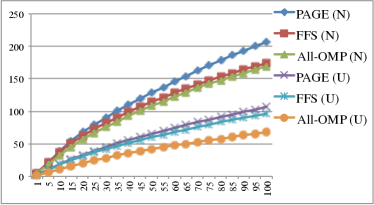
(c) TV with $c_{a}=0.1$	(d) TV with $c_{a}=0.001$

Figure 6: Expected profit achieved (Y-axis) on Flixster graphs w.r.t. $|S|$ (X-axis). (N)/(U) denotes normal/uniform distribution.

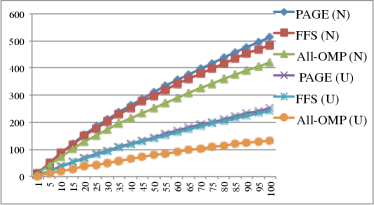
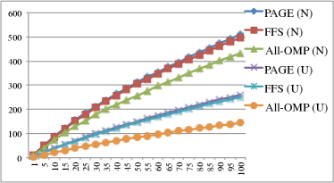
(a) WD with $c_{a}=0.1$	(b) WD with $c_{a}=0.001$
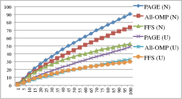
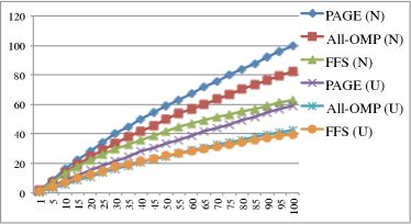
(c) TV with $c_{a}=0.1$	(d) TV with $c_{a}=0.001$

Figure 7: Expected profit achieved (Y-axis) on NetHEPT graphs w.r.t. $|S|$ (X-axis). (N)/(U) denotes normal/uniform distribution.

Expected Profit Achieved.

The quality of outputs (seed sets and price vectors) of All-OMP, FFS, and PAGE for general ProMax are evaluated based on the expected profit achieved. Fig. 5, 6, and 7 illustrate the results on Epinions, Flixster, and NetHEPT, respectively. On each network, both valuation distributions are tested in four settings: WD weights with $c_{a}=0.1$ and $0.001$; TV weights with $c_{a}=0.1$ and $0.001$. As prices and valuations are in $[0,1]$, we use $0.1$ to simulate high acquisition costs and $0.001$ for low costs. Except for NETHEPT-TV with $c_{a}=0.1$ (Fig. 7c) and $0.001$ (Fig. 7d), FFS is better than All-OMP; this indicates that only in NetHEPT-TV, influence is low enough so that giving free samples blindly to all seeds do impair profits.

In all test cases, PAGE performed consistently better than FFS and All-OMP. The margin between PAGE and FFS is higher in TV graphs (by, e.g., $15\%$ on Epinions-TV with $\mathcal{N}(0.53,0.14^{2})$, $c_{a}=0.1$) than that in WD graphs (by, e.g., $2.1\%$ on Epinions-WD with $\mathcal{N}(0.53,0.14^{2})$, $c_{a}=0.1$), as higher influence in WD graphs can potentially bring more compensations for profit loss in seeds for FFS. Also, the expected profit of all algorithms under $\mathcal{N}(0.53,0.14^{2})$ is higher than that under $\mathcal{U}(0,1)$, since adoption probabilities under $\mathcal{N}(0.53,0.14^{2})$ are higher.

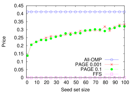
Figure 8: Price assigned to seeds (Y-axis) w.r.t. $|S|$ (X-axis) on Epinions-TV with $\mathcal{N}(0.53,0.14^{2})$.

Price Assignments.

For $\mathcal{N}(0.53,0.14^{2})$ and $\mathcal{U}(0,1)$, the OMP is $0.41$ and $0.5$, respectively. Fig. 8 demonstrates the prices offered to each seed by All-OMP, FFS, and PAGE on Epinions-TV with $\mathcal{N}(0.53,0.14^{2})$. All-OMP and FFS assigns $0.41$ and $0$ for all seeds, respectively, For PAGE, as the seed set grows, price tends to increase, reflecting the intuition that discount is proportional to the influence (profit potential) of seeds, as they are added in a greedy fashion and those added later have diminishing profit potential.

Algorithm	Epinions-WD		Flixster-WD		NetHEPT-WD
	$\mathcal{N}$	$\mathcal{U}$	$\mathcal{N}$	$\mathcal{U}$	$\mathcal{N}$	$\mathcal{U}$
All-OMP	6.7	2.3	3.0	1.0	2.6	2.2
FFS	6.3	2.1	2.8	1.0	2.7	2
PAGE	4.8	1.3	2.3	0.5	1.0	0.9

Table 2: Running time in hours (WD weights, $c_{a}=0.1$)

Algorithm	Epinions-TV		Flixster-TV		NetHEPT-TV
	$\mathcal{N}$	$\mathcal{U}$	$\mathcal{N}$	$\mathcal{U}$	$\mathcal{N}$	$\mathcal{U}$
All-OMP	5.1	2.4	1.4	1.0	2.3	2.1
FFS	5.5	2.5	1.5	0.8	2.2	1.8
PAGE	4.0	1.0	0.9	0.4	0.8	0.5

Table 3: Running time in hours (TV weights, $c_{a}=0.1$)

Running Time.

Tables 2 and 3 present the running time of all algorithms on the three networks with WD weights and TV weights, respectively. As adoption probabilities under $\mathcal{N}(0.53,0.14^{2})$ are higher, all algorithms ran longer with the normal distribution on all graphs. Similarly, as influence in WD graphs are higher, the running time on them is longer than that on TV graphs.

All-OMP and FFS have roughly the same running time. More interestingly, PAGE is faster than both baselines in all cases. The observation is that in each round of U-Greedy, PAGE maximizes the marginal profit for each candidate seed in the priority queue maintained by CELF. Thus, heuristically, the lazy-forward procedure in CELF (see [18]) has a better chance to return the best candidate seed sooner for PAGE. All-OMP and FFS also benefit from CELF, but since the marginal profits of candidate seeds are often suboptimal, elements in the CELF queue tend to be clustered, and thus the lazy-forward is not as effective. Besides, for PAGE under $\mathcal{N}(0.53,0.14^{2})$, the golden section search usually converges in less than $40$ iterations with stopping criteria $10^{-8}$ (defined in Sec. 4.2); thus the extra overhead it brings is negligible compared to MC simulations.

To conclude, our empirical results on three real-world datasets with two different valuation distributions demonstrate that the PAGE algorithm consistently outperforms baselines All-OMP and FFS in both expected profit achieved and running time. It is also the most robust (against various inputs) among all algorithms.

6 Conclusions and Discussions

In this work, we extend the classical LT model by incorporating prices and valuations to capture monetary aspects in product adoption, which we distinguish from social influence. We study the profit maximization (ProMax) problem under our proposed LT-V model, and prove NP-hardness and submodularity results. We propose the PAGE algorithm which dynamically determines the prices for nodes based on their profit potential. Our experimental results show that PAGE outperforms the baselines in all aspects evaluated.

For future work, first, the added ingredients for LT-V can be used to extend models like IC [16] and LT-C [2]. Second, the current algorithms cannot scale to larger graphs due to expensive MC simulations. To achieve scalability, we can replace the MC simulations with fast heuristics for the LT model, e.g., LDAG [6] and SimPath [12].

Another extension is to consider users’ spontaneous interests in product adoption, and incorporate it into the LT-V model for profit maximization. Due to personal demand, a user may have spontaneous interests in a certain product even when no neighbor in the network has adopted. To model this, each node $u_{i}$ is associated with a “network-less” probability $\delta_{i}$ [7]. An inactive node becomes influenced when the sum of $\delta_{i}$ and the total influence from its adopting neighbors are at least $\theta_{i}$. A marketing company can thus wait for spontaneous adopters to emerge first and propagate their adoption (for $\ell$ time steps, where $\ell$ is the diameter of $G$), and then deploy a viral marketing campaign to maximize the expected profit. Our analysis and solution framework (Secs. 3, 4) can be naturally applied to this setting.

In addition, it is interesting to look into more sophisticated methodologies to acquire knowledge on user valuations, e.g., by leveraging users’ full previous transaction history, as well as look at real datasets besides Epinions.com.

References

- [1] D. Arthur, R. Motwani, A. Sharma, and Y. Xu. Pricing strategies for viral marketing on social networks. In WINE, pages 101–112, 2009.
- [2] S. Bhagat, A. Goyal, and L. V. S. Lakshmanan. Maximizing product adoption in social networks. In WSDM, pages 603–612, 2012.
- [3] F. Bloch and N. Quérou. Pricing in networks. Working papers, unpublished, Ecole Polytechnique, Oct. 2011.
- [4] W. Chen, P. Lu, X. Sun, B. Tang, Y. Wang, and Z. A. Zhu. Optimal pricing in social networks with incomplete information. In WINE, pages 49–60, 2011.
- [5] W. Chen, C. Wang, and Y. Wang. Scalable influence maximization for prevalent viral marketing in large-scale social networks. In KDD, pages 1029–1038, 2010.
- [6] W. Chen, Y. Yuan, and L. Zhang. Scalable influence maximization in social networks under the linear threshold model. In ICDM, pages 88–97, 2010.
- [7] P. Domingos and M. Richardson. Mining the network value of customers. In KDD, pages 57–66, 2001.
- [8] U. Feige, V. S. Mirrokni, and J. Vondrak. Maximizing non-monotone submodular functions. In FOCS, pages 461–471, 2007.
- [9] C. F. Gerald and P. O. Wheatley. Applied numerical analysis (7th ed.). Addison-Wesley, 2004.
- [10] T. F. Gonzalez, S. Sahni, and W. R. Franta. An efficient algorithm for the kolmogorov-smirnov and lilliefors tests. ACM Trans. Math. Softw., 3(1):60–64, 1977.
- [11] A. Goyal, W. Lu, and L. V. S. Lakshmanan. Celf++: optimizing the greedy algorithm for influence maximization in social networks. In WWW, 2011.
- [12] A. Goyal, W. Lu, and L. V. S. Lakshmanan. Simpath: An efficient algorithm for influence maximization under the linear threshold model. In ICDM, pages 211–220, 2011.
- [13] J. D. Hartline, V. S. Mirrokni, and M. Sundararajan. Optimal marketing strategies over social networks. In WWW, pages 189–198, 2008.
- [14] A. X. Jiang and K. Leyton-Brown. Estimating bidders’ valuation distributions in online auctions. In Workshop on Game Theory and Decision Theory (GTDT) at IJCAI, 2005.
- [15] S. Kalish. A new product adoption model with price, advertising, and uncertainty. Management Science, 31(12):1569–1585, 1985.
- [16] D. Kempe, J. M. Kleinberg, and É. Tardos. Maximizing the spread of influence through a social network. In KDD, pages 137–146, 2003.
- [17] R. D. Kleinberg and F. T. Leighton. The value of knowing a demand curve: Bounds on regret for online posted-price auctions. In FOCS, pages 594–605, 2003.
- [18] J. Leskovec, A. Krause, C. Guestrin, C. Faloutsos, J. M. VanBriesen, and N. S. Glance. Cost-effective outbreak detection in networks. In KDD, pages 420–429, 2007.
- [19] G. L. Nemhauser, L. A. Wolsey, and M. L. Fisher. An analysis of approximations for maximizing submodular set functions. Mathematical Programming, 14(1):265–294, 1978.
- [20] M. Richardson and P. Domingos. Mining knowledge-sharing sites for viral marketing. In KDD, pages 61–70, 2002.
- [21] Y. Shoham and K. Leyton-Brown. Multiagent Systems - Algorithmic, Game-Theoretic, and Logical Foundations. Cambridge University Press, 2009.