Rate of convergence for Cardy’s formula

Abstract.

We show that crossing probabilities in 2D critical site percolation on the triangular lattice in a piecewise analytic Jordan domain converge with power law rate in the mesh size to their limit given by the Cardy-Smirnov formula. We use this result to obtain new upper and lower bounds of $e^{O(\sqrt{\log\log R})}R^{-1/3}$ for the probability that the cluster at the origin in the half-plane has diameter $R$, improving the previously known estimate of $R^{-1/3+o(1)}$.

1. Introduction

Let $\Omega\subset\mathbb{C}$ be a nonempty Jordan domain, and let $A,B,C,D$ be four points on $\partial\Omega$ ordered counter-clockwise. Let $P^{\delta}$ denote the critical site percolation measure on the triangular lattice with mesh size $\delta>0$, that is, each site in the lattice is independently declared open or closed with probability $1/2$ each. The Cardy-Smirnov formula [Sm01] states that as $\delta\to 0$, the probability $P^{\delta}(AB\leftrightarrow CD)$ that there exists a path of open sites in $\Omega$ starting at the arc $AB$ and ending at the arc $CD$ converges to a limit that is a conformal invariant of the four-pointed domain (see Figure 1). Our main theorem establishes a power law rate for this convergence under mild regularity hypotheses.

Theorem 1.1.

Let $(\Omega,A,B,C,D)$ be a four-pointed Jordan domain bounded by finitely many analytic arcs meeting at positive interior angles. There exists $c>0$ such that

$$P^{\delta}(AB\leftrightarrow CD)-\lim_{\delta\to 0}P^{\delta}(AB\leftrightarrow CD)=O(\delta^{c}),$$

where the implied constants depend only on $(\Omega,A,B,C,D)$.

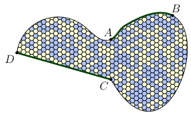
Figure 1. We picture triangular site percolation by coloring the faces of the dual hexagonal lattice. Smirnov’s theorem states that the probability of a yellow crossing from boundary arc $AB$ to boundary arc $CD$ converges, as the mesh size tends to 0, to a limit which is a conformal invariant of the four-pointed domain $(\Omega,A,B,C,D)$. In the sample shown, the yellow crossing event $\{AB\leftrightarrow CD\}$ occurs.

We prove Theorem 1.1 for all $c<1/6$, with better exponents for certain domains (see Remark 2.2).

Schramm posed the problem of improving estimates on percolation arm events (see Problem 3.1 in [S07]). In Section 6, we obtain the following improvement of the estimate found in [SW01] for the probability that the origin is connected to $\{z\,:\,|z|=R\}$ in the upper half-plane.

Theorem 1.2.

Let $\{0\leftrightarrow S_{R}\}$ denote the event that there exists an open path from the origin to the semicircle $S_{R}$ of radius $R$ in critical site percolation on the triangular lattice in the half-plane. Then

$$\mathbb{P}(0\leftrightarrow S_{R})=e^{O(\sqrt{\log\log R})}R^{-1/3}=(\log R)^{O(1/\sqrt{\log\log R})}R^{-1/3}.$$

Our methods also yield the estimate $e^{O(\sqrt{\log\log R})}R^{-1/6\beta}$ for the probability that the origin is connected to $\{z\,:\,|z|=R\}$ in the sector centered at the origin of angle $2\pi\beta$. We remark that our methods are insufficient to give better estimates for the probability that the origin is connected to $\{z\,:\,|z|=R\}$ in the full plane (the so-called one-arm exponent, which takes the value $5/48$, [LSW01]) and multiple arm events either in the full or half plane.

In his proof of Cardy’s formula, Smirnov constructs a discrete observable $G_{\delta}:\Omega^{\delta}\to\mathbb{C}$, defined as a complex linear combination of crossing probabilities, and shows that $G_{\delta}$ converges as $\delta\to 0$ to a conformal map. The crossing probabilities and their limits can be then read off $G_{\delta}$ and its limit. A similar high-level strategy was also used by Smirnov [Sm10] and Chelkak and Smirnov [CS12] to show that the interfaces of the critical Ising and FK-Ising model converge to SLE curves. See [DS12] for a comprehensive survey of this subject.

We note that the power law rate of convergence is obtained for the FK-Ising model ([Sm10, HS12]) more directly than for percolation, because the combinatorial relations in the Ising model establish that “discrete Cauchy-Riemann” equations hold precisely. In particular, in the case of the Ising model one can work with discrete second derivatives and obtain discrete harmonic functions. By contrast, for percolation the observable $G_{\delta}$ is only known to be approximately analytic. Thus it is necessary to control the global effects of these local deviations from exact analyticity. To accomplish this, we use a Cauchy integral formula with an elliptic function kernel in place of the usual $z\mapsto 1/z$.

The half-plane arm exponent, as well as the validity of Smirnov’s theorem is widely believed to be universal in the sense that it should hold for any reasonable two-dimensional lattice. Nevertheless, so far it is an open problem to prove Smirnov’s theorem even for the case of bond percolation on the square lattice. The value of the exponent does, however, depend on the dimension. For example, in high dimensions (that is, dimension at least $19$ in the usual nearest-neighbor lattice, or dimension at least $6$ on lattices which are spread-out enough) its value is $-3$ [KN]. To the best of our knowledge, there are no predictions in dimensions $3,4,5$. As for the error terms, in dimension 2 it is believed that the correct bound for $\mathbb{P}(0\leftrightarrow S_{R})$ of Theorem 1.2 is $\Theta(R^{-1/3})$ (we are unable to prove this here). In general, it is believed that the polynomial decay should have no logarithmic corrections except for at dimension $6$, the upper critical dimension (see [SA94]).

Finally, we remark that Theorem 1.1 has been independently proved by Binder, Chayes, and Lei [BCL12] using different methods. Their approach applies to arbitrary simply connected domains, while our proof achieves explicit exponents for the subclass of piecewise analytic domains (see Remark 2.2).

2. Set-up and notation

Throughout the paper, we consider piecewise analytic Jordan domains $\Omega$ with positive interior angles. That is, $\partial\Omega$ is a Jordan curve which can be written as the concatenation of finitely many analytic arcs $\gamma_{1},\ldots,\gamma_{N}$. Recall that an arc is said to be analytic if it can be realized as the image of a closed subinterval $I\subset\mathbb{R}$ under a real-analytic function from $I$ to $\mathbb{C}$. We will call the point at which two such arcs meet a corner, and we will denote the collection of corners by $\{x_{j}\}_{j=1,\ldots,N}$. Our hypotheses imply that there is a well-defined interior angle at each corner, and we impose the condition that each such angle lies in $(0,2\pi]$. We define $\tau\colonequals\exp(2\pi i/3)$ and let $\Omega$ have three marked boundary points, labeled $x(1)$, $x(\tau)$, and $x(\tau^{2})$ in counter-clockwise order. We denote the angles at marked points by $2\pi\alpha_{j}$ and those at unmarked points by $2\pi\beta_{i}$.

Denote by $\Omega^{\delta}$ the sites of the triangular lattice with mesh size $\delta$ which are contained in $\Omega$ or have a neighbor contained in $\Omega$ and consider critical site percolation on $\Omega^{\delta}$. Let $(\Omega^{\delta})^{*}$ be the sites of the hexagonal lattice dual to $\Omega^{\delta}$ (that is, $(\Omega^{\delta})^{*}$ are the centers of the triangles of $\Omega^{\delta}$). We depict open and closed sites by coloring the corresponding hexagonal faces yellow and blue, respectively. For $z,z^{\prime}\in\partial\Omega$, let $[z,z^{\prime}]$ denote the counter-clockwise boundary arc from $z$ to $z^{\prime}$. As in [Sm01], the following events play a central role (see Figure 2):

$$E^{\delta}_{\tau^{k}}(z)=\left\{\begin{array}[]{c}\exists\text{ a simple open path from }[x(\tau^{k+2}),x(\tau^{k})]\text{ to }[x(\tau^{k}),x(\tau^{k+1})]\\ \text{ separating }z\text{ from }[x(\tau^{k+1}),x(\tau^{k+2})]\end{array}\right\}\,,$$

for $k\in\{0,1,2\}$. Let $H_{\tau^{k}}^{\delta}=\mathbb{P}(E_{\tau^{k}}^{\delta})$ and for $z$ and $z+\eta$ neighbors in $(\Omega^{\delta})^{*}$, define $P^{\delta}_{\tau^{k}}(z,\eta)$ $=\mathbb{P}(E_{\tau^{k}}^{\delta}(z+\eta)\setminus E_{\tau^{k}}^{\delta}(z))$. Following [B07], we define

$$G^{\delta}\colonequals H^{\delta}_{1}+\tau H^{\delta}_{\tau}+\tau^{2}H^{\delta}_{\tau^{2}},\qquad S^{\delta}\colonequals H^{\delta}_{1}+H^{\delta}_{\tau}+H^{\delta}_{\tau^{2}}.$$

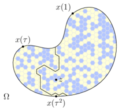
Figure 2. The event $E^{\delta}_{1}(z)$ occurs when there exists a simple open path separating $z$ from $[x(\tau),x(\tau^{2})]$.

We extend the domain of $G^{\delta}$ from the lattice $(\Omega^{\delta})^{*}$ to all of $\Omega$ by triangulating each hexagonal face and linearly interpolating in each resulting triangle. The possible triangulations for each face are and and rotations thereof. We will see that the choice of triangulation is immaterial. We obtain Theorem 1.1 as a corollary of the following theorem.

Theorem 2.1.

Let $(\Omega,x(1),x(\tau),x(\tau^{2}))$ be a three-pointed, simply connected Jordan domain bounded by finitely many analytic arcs meeting at positive interior angles, and let $T$ be the triangular domain with vertices $1,\tau,$ and $\tau^{2}$. Then there exists $c>0$ so that $|G^{\delta}(z)-\phi(z)|=O(\delta^{c})$, where $\phi$ is the conformal map from $(\Omega,x(1),x(\tau),x(\tau^{2}))$ to $(T,1,\tau,\tau^{2})$, and where the implied constants depend only on the three-pointed domain.

Remark 2.2.

Our methods establish Theorem 2.1 (and thus Theorem 1.1) for any exponent

(2.1) $$c<\min_{i,j}\left(\frac{2}{3},\frac{1}{6\alpha_{i}},\frac{1}{2\beta_{j}}\right).$$

These exponents are essentially the best possible given our approach, because no piecewise-linear interpolant of a function on a lattice of mesh $\delta$ can approximate the conformal map to $T$ with error better than $\delta^{\min_{i,j}(1/6\alpha_{i},1/2\beta_{j})}$ due to behavior near the boundary.

Remark 2.3.

Our proof of Theorem 1.1 uses results whose proofs require SLE tools, but only for two purposes: (1) to handle the case where the domain contains reflex angles (that is, some interior angle formed at the intersection of two of the bounding analytic arcs is greater than $\pi$), and (2) to obtain the sharp exponent discussed in Remark 2.2. Without SLE machinery, we obtain Theorem 1.1 for domains without reflex angles and for exponents $c<\min_{i,j}(c_{3},1/6\alpha_{i},1/6\beta_{j})$, where $c_{3}$ is the three-arm whole-plane exponent (which is known to be 2/3, but only by using an SLE convergence result). See Remark 5.3 for further discussion of this point.

Remark 2.4.

In [SW01], a bound of $R^{-1/3+o(1)}$ for the half-plane arm exponent was proved using SLE calculations and the fact that the percolation exploration path converges to SLE₆ as proved by Smirnov [Sm01] and Camia-Newman [CN07]. By contrast, our proof follows from Proposition 5.6, which is a variation of Theorem 1.1 proved by similar methods. The only SLE result on which our proof of Theorem 1.2 depends is the statement $c_{3}>1/3$, where $c_{3}$ is the three-arm whole-plane exponent.

For two quantities $f(\delta)$ and $g(\delta)$, we use the usual asymptotic notation $f=O(g)$ to mean that there exist constants $C$ and $\delta_{0}>0$ so that $|f(\delta)|\leq C|g(\delta)|$ for all $0<\delta<\delta_{0}$. We use the notation $f\lesssim g$ to mean $f=O(g)$ as $\delta\to 0$, and we write $f\asymp g$ to mean $f=O(g)$ and $g=O(f)$. We sometimes use $C$ to denote an arbitrary constant.

3. Preliminaries

First we recall some results from [Sm01]. The first is a Hölder norm estimate of $H_{\tau^{k}}$ and is obtained via Russo-Seymour-Welsh estimates.

Lemma 3.1 (Lemma 2.2 in [Sm01]).

There exist $C,c>0$ depending only on $\Omega$ such that for all $\delta>0$, the $c$-Hölder norm of $H_{\tau^{k}}^{\delta}$ is bounded above by $C$. That is,

(3.1) $$|H^{\delta}_{\tau^{k}}(z)-H^{\delta}_{\tau^{k}}(z^{\prime})|\leq C|z-z^{\prime}|^{c},$$

for ${\tau^{k}}\in\{1,\tau,\tau^{2}\}$.

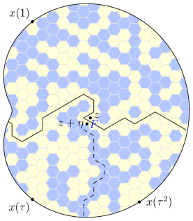
Figure 3. The event $E_{1}(z)\setminus E_{1}(z+\eta)$ occurs if and only if there are disjoint yellow arms from $z$ to $[x(\tau^{2}),x(1)]$ and from $z$ to $[x(1),x(\tau)]$ forming a simple path separating $z$ from $[x(\tau),x(\tau^{2})]$, as well as a blue arm from $z+\eta$ to $[x(\tau),x(\tau^{2})]$ which prevents a yellow path from separating $z+\eta$ as well.

Our second estimate is Smirnov’s “color switching” lemma.

Proposition 3.2 (Lemma 2.1 in [Sm01]).

For every vertex $z\in(\Omega^{\delta})^{*}$ and $k\in\{0,1,2\}$, we have

$$P^{\delta}_{\tau^{k}}(z,\eta)=P^{\delta}_{\tau^{k+1}}(z,\tau\eta).$$

We will sometimes drop the superscript $\delta$ from the notation when it’s clear from context. If $F$ is a hexagonal face in $(\Omega^{\delta})^{*}$, let $V(F)$ denote the set of vertices of $F$ and define for each $z\in V(F)$ the vector $\eta$ pointing to the adjacent vertex counterclockwise from $z$. Define the difference (see Figure 4(a))

$$R_{k}(z)\colonequals|P_{\tau^{k}}(z+\tau^{k}\eta,-\tau^{k}\eta)-P_{\tau^{k}}(z+\tau^{k+1}\eta,-\tau^{k}\eta)|.$$

Define $z^{\prime}=z+\tau\eta-\eta$ and rewrite $P_{\tau^{k}}(z^{\prime},\eta)$ as $P^{\Omega^{\prime}}_{\tau^{k}}(z,\eta)$, where $\Omega^{\prime}$ is obtained by translating $\Omega$ by $z-z^{\prime}$ (and $P^{\Omega^{\prime}}$ refers to probability with respect to $\Omega^{\prime}$). Define the events $E_{\tau^{k}}^{\prime}(z)$ with respect to $\Omega^{\prime}$, and define $x^{\prime}(\tau^{k})$ to be $x(\tau^{k})$ translated by $z-z^{\prime}$.

Given $k,l\in\{0,1,2\}$, $\sigma\in\{-1,1\}$, and $z\in(\Omega^{\delta})^{*}$, we say that the event $E^{\text{five arm}}_{\tau^{k},\tau^{l},\sigma}(z)$ occurs if

• $\sigma=1$, and $E_{\tau^{k}}(z)\setminus E_{\tau^{k}}(z+\tau^{k}\eta)$ occurs, and the arm from $z$ to
  $[x(\tau^{l+1}),x(\tau^{l+2})]$ fails to connect in $\Omega^{\prime}$, or

• $\sigma=-1$, and $E^{\prime}_{\tau^{k}}(z)\setminus E^{\prime}_{\tau^{k}}(z+\tau^{k}\eta)$ occurs, and the arm from $z$ to
  $[x^{\prime}(\tau^{l+1}),x^{\prime}(\tau^{l+2})]$ fails to connect in $\Omega$.

For $z_{0}\in\Omega$, we define $E^{\text{five arm}}_{\tau^{k},\tau^{l},\sigma}(z)$ to be the union of $E^{\text{five arm}}_{\tau^{k},\tau^{l},\sigma}(z)$ as $z$ ranges over the vertices of the hexagonal face containing $z_{0}$.

Note that these are indeed five-arm events because two additional arms are required to prevent the failed arm from connecting elsewhere on $[x(\tau^{l}),x(\tau^{l+1})]$ (see Figure 5).

Proposition 3.3.

If $F$ is a hexagonal face in $(\Omega^{\delta})^{*}$, then for $z_{0}$ in the interior of $F$ we have

(3.2) $$\delta|\bar{\partial}G^{\delta}(z_{0})| \leq 3\sqrt{3}\max_{z\in V(F),\,k\in\{0,1,2\}}R_{k}(z)$$

(3.3) $$\leq 54\sqrt{3}\max_{k,l\in\{0,1,2\},\sigma\in\{-1,1\}}\mathbb{P}(E_{\tau^{k},\tau^{l},\sigma}^{\text{five arm}}(z_{0})).$$

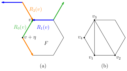
Figure 4. (a) Each arrow represents the probability of a three-arm event as shown in Figure 3. The quantity $R_{0}(z)$ is defined to be the difference between the probabilities represented by the two green arrows. Similarly, $R_{1}(z)$ is shown in blue and $R_{2}(z)$ is shown in orange. (b) Suppose that the triangle $z_{1}z_{2}z_{3}$ is in the triangulation of the face $F$. For $z$ in the interior of this triangle, we bound $\bar{\partial}G^{\delta}(z)$ by applying (3.4) to triangles $z_{2}z_{1}z_{4}$ and $z_{1}z_{4}z_{3}$.

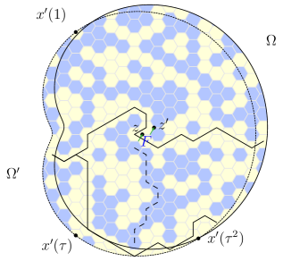
Figure 5. The symmetric difference of the events $E_{1}(z)\setminus E_{1}(z+\eta)$ and $E^{\prime}_{1}(z^{\prime})\setminus E^{\prime}_{1}(z^{\prime}+\eta)$ can occur in six ways. One way for the event to occur is shown above: the three requisite arms are present in $\Omega$, so the event $E_{1}(z)\setminus E_{1}(z+\eta)$ occurs. However, the blue arm fails to connect to $[x^{\prime}(\tau),x^{\prime}(\tau^{2})]$ in $\Omega^{\prime}$. This requires two additional yellow arms to prevent the blue arm from connecting elsewhere on $[x^{\prime}(\tau),x^{\prime}(\tau^{2})]$. This event is denoted $E^{\text{five arm}}_{1,1,1}(z)$. The first subscript $\tau^{k}$ specifies that the three-arm event under consideration involves the blue arm touching down on $[x(\tau^{k+1}),x(\tau^{k+2})]$. The second subscript $\tau^{l}$ indicates that the boundary arc $[x(\tau^{l+1}),x(\tau^{l+2})]$ is involved in a failed connection. The third subscript $\sigma$ describes whether the failed connection occurs in $\Omega$ but not $\Omega^{\prime}$ (in which case we say $\sigma=1$), or vice versa ($\sigma=-1$).

Proof.

The main idea in the following proof is suggested in [Sm01]. For (3.2), we first observe that for $z\in V(F)$, we have

$$\delta\left[\frac{\partial}{\partial\eta}H_{\tau^{k}}(z)-\frac{\partial}{\partial(\tau\eta)}H_{\tau^{k+1}}(z)\right] =P_{\tau^{k}}(z,\eta)-P_{\tau^{k}}(z+\eta,-\eta)$$

$$\hskip 56.9055pt-P_{\tau^{k+1}}(z,\tau\eta)+P_{\tau^{k+1}}(z+\tau\eta,-\tau\eta)$$

$$=P_{\tau^{k+1}}(z+\tau\eta,-\tau\eta)-P_{\tau^{k}}(z+\eta,-\eta)$$

$$=P_{{\tau^{k}}}(z+\tau\eta,-\eta)-P_{\tau^{k}}(z+\eta,-\eta),$$

by Proposition 3.2. Suppose that the triangle $T$ with vertices $z$, $z+\eta$, and $z+\tau\eta$ is in the triangulation of $F$. Then for $z$ in the interior of $T$, we may write $\delta\bar{\partial}$ as $\delta\lambda\left(\frac{\partial}{\partial\eta}-\frac{1}{\tau}\frac{\partial}{\partial(\tau\eta)}\right)$, where $\lambda=1/2+i/(2\sqrt{3})$. We obtain

$$\delta\left|\lambda\left(\frac{\partial}{\partial\eta}-\frac{1}{\tau}\right.\right. \left.\left.\frac{\partial}{\partial(\tau\eta)}\right)\vphantom{\frac{\partial}{\partial\eta}}(H_{1}+\tau H_{\tau}+\tau^{2}H_{\tau^{2}})\right|$$

$$=|\lambda|\left|\left(\frac{\partial H_{1}}{\partial\eta}-\frac{\partial H_{\tau}}{\partial\tau\eta}\right)+\tau\left(\frac{\partial H_{\tau}}{\partial\tau\eta}-\frac{\partial H_{\tau^{2}}}{\partial\tau^{2}\eta}\right)+\tau^{2}\left(\frac{\partial H_{\tau}^{2}}{\partial\tau^{2}\eta}-\frac{\partial H_{1}}{\partial\eta}\right)\right|$$

(3.4) $$\leq\sqrt{3}\max_{k\in\{0,1,2\}}\left|P_{\tau^{k}}(z+\tau^{k}\eta,-\tau^{k}\eta)-P_{\tau^{k}}(z+\tau^{k+1}\eta,-\tau^{k}\eta)\right|.$$

For triangles whose vertices are not consecutive vertices of the hexagon, we obtain a similar bound by applying (3.4) two or three times (see Figure 4(b)).

For the bound in (3.3), we let $A=E_{\tau^{k}}(z)\setminus E_{\tau^{k}}(z+\tau^{k}\eta)$ and $B=E^{\prime}_{\tau^{k}}(z)\setminus E^{\prime}_{\tau^{k}}(z+\tau^{k}\eta)$ and apply $|\mathbb{P}(A)-\mathbb{P}(B)|\leq\mathbb{P}(A\bigtriangleup B),$ where $A\bigtriangleup B$ denotes the symmetric difference of $A$ and $B$. Note that $A\bigtriangleup B\subset\bigcup_{k,l,\sigma}E^{\text{five arm}}_{\tau^{k},\tau^{l},\sigma}(z_{0})$, since some arm in $\Omega$ must fail to connect in $\Omega^{\prime}$, or vice versa. Applying a union bound as $k$ and $l$ range over $\{0,1,2\}$ and $\sigma$ ranges over $\{-1,1\}$ yields the result. ∎

Finally, we need the following a priori estimates for $H_{\tau^{k}}(z)$ when $z$ is near $\partial\Omega$.

Proposition 3.4.

Let $(\Omega,x(1),x(\tau),x(\tau^{2}))$ be a three-pointed Jordan domain. There exists $c>0$ such that for every $z\in(\Omega_{\delta})^{*}$ which is closer to $[x(\tau^{k+1}),x(\tau^{k+2})]$ than to $\partial\Omega\setminus[x(\tau^{k+1}),x(\tau^{k+2})]$, the following statements hold.

1. $H_{\tau^{k}}(z)\lesssim\operatorname{dist}(z,\partial\Omega)^{c}$.

2. $|S(z)-1|\lesssim\operatorname{dist}(z,\partial\Omega)^{c}$.

3. $\operatorname{dist}(G^{\delta}(z),[x(\tau^{k+1}),x(\tau^{k+2})])\lesssim\operatorname{dist}(z,[\tau^{k+1},\tau^{k+2}])^{c}$,

with implied constants depending only on $(\Omega,x(1),x(\tau),x(\tau^{2}))$.

Proof.

(i) For $w\in[x(\tau^{k+1}),x(\tau^{k+2})]$, define $D_{1}(w)$ and $D_{2}(w)$ to be the distances from $w$ to the boundary arcs $[x(\tau^{k+2}),x(\tau^{k})]$ and $[x(\tau^{k}),x(\tau^{k+1})]$, respectively. Let $D=\inf_{w\in[x(\tau^{k+1}),x(\tau^{k+2})]}\max(D_{1}(w),D_{2}(w))>0$. Let $z^{\prime}\in[x(\tau^{k+1}),x(\tau^{k+2})]$ be a closest point to $z$, and consider the annulus centered at $z^{\prime}$ with inner radius $|z-z^{\prime}|$ and outer radius $R$. Then $E_{\tau^{k}}(z)$ entails a crossing of this annulus, which has probability $O(|z-z^{\prime}|^{c})$ by Russo-Seymour-Welsh.

(ii) Again let $z^{\prime}\in[x(\tau^{k+1}),x(\tau^{k+2})]$ be a point nearest to $z$. Consider the event that there is a yellow crossing from $[x(\tau^{k+2}),x(\tau^{k})]$ to $[x(\tau^{k+1}),z^{\prime}]$ and the event that there is a blue crossing from $[x(\tau^{k}),x(\tau^{k+1})]$ to $[z^{\prime},x(\tau^{k+2})]$. These events are mutually exclusive, and their union has probability 1. Since these two events have probability $H_{\tau^{k+1}}(z)$ and $H_{\tau^{k+2}}(z)$, we see that

$$H_{\tau^{k}}(z)+(H_{\tau^{k+1}}(z)+H_{\tau^{k+2}}(z)) =O((\operatorname{dist}(z,\partial\Omega)^{c})+1.$$

(iii) This statement says that $G$ maps points near each boundary arc to the corresponding image segment in the triangle, and it follows directly from (i). ∎

3.1. Percolation Estimates

In this subsection we present several percolation-related estimates in preparation for the proof of Theorem 2.1. We think of these lattices as embedded in $\mathbb{R}^{2}$ with mesh size $\delta$, and distances are measured in the Euclidean metric.

Define $\mathcal{C}^{k}_{\theta}(r,R)$ to be the event that there exist $k$ disjoint crossings of alternating colors from the inner to the outer boundary of an annular section $A_{\theta}(r,R)$ of angle $\theta$ and inner radius $r$ and outer radius $R$. The following is a well-known result on the half-annulus two-arm and three-arm exponents. We refer the reader to [LSW01, Appendix A] for a proof.

Proposition 3.5.

We have

$$P^{\delta}(\mathcal{C}^{2}_{\pi}(r,R)) \asymp\frac{r}{R},\text{ and}$$

$$P^{\delta}(\mathcal{C}^{3}_{\pi}(r,R)) \asymp\left(\frac{r}{R}\right)^{2}.$$

In the next proposition, we show that the exponents in the estimates above are continuous in the angle $\theta$.

Proposition 3.6.

For all $\epsilon>0$, there exists $\alpha=\alpha(\epsilon)>0$ so that

(3.5) $$P^{\delta}(\mathcal{C}^{2}_{\pi+\alpha}(r,R)) \lesssim\left(\frac{r}{R}\right)^{1-\epsilon},\text{ and}$$

(3.6) $$P^{\delta}(\mathcal{C}^{3}_{\pi+\alpha}(r,R)) \lesssim\left(\frac{r}{R}\right)^{2-\epsilon},$$

with implied constants depending only on $\epsilon$.

Proof.

We only prove (3.5) since the proof of (3.6) is essentially the same. We begin by showing that there exists $C>0$ so that for all $r>0$ and $R>0$, there exists $\delta_{0}=\delta_{0}(r,R,\epsilon)>0$ for which $P^{\delta}(\mathcal{C}^{2}_{\pi+\alpha}(r,R))\leq C\left(\frac{r}{R}\right)^{1-\epsilon}$ holds when $0<\delta<\delta_{0}$. For this statement, we may assume without loss of generality that $R=1$.

Consider the sector of angle $\pi+\alpha$ as a union of a sector of angle $\pi$ with a sector of angle $\alpha$. Divide the sector of angle $\alpha$ into $\lceil(1-r)\alpha^{-1}\rceil$ curvilinear quadrilaterals of radial dimension $\alpha$, as shown in Figure 6. Let $s\in\{1,\ldots,\lceil(1-r)\alpha^{-1}\rceil\}$ and note that the event $\mathcal{C}^{2}_{\pi+\alpha}(r,1)\setminus\mathcal{C}^{2}_{\pi}(r,1)$ entails the existence of a quadrilateral of distance $s\alpha$ from the inner circle of radius $r$ such that there is a three-arm crossing of alternating colors of the half-annulus with inner radius $\alpha$ and outer radius $s\alpha\wedge(1-r-(s+1)\alpha)$.

In the case $s\alpha\leq(1-r)/2$, there is also a two-arm crossing from the annulus of inner radius $s\alpha$ and outer radius $s\alpha+r$ (see Figure 6(a)). If $s\in[2^{k},2^{k+1}]$ and $s\alpha\leq(1-r)/2$, then the probability that both of these events occur is $O\left(\left(\frac{\alpha}{s\alpha}\right)^{2}\left(\frac{\alpha}{\alpha s+r}\right)\right)=O(\frac{\alpha}{2^{k}})$ by Proposition 3.5. Applying a union bound over $s$ we obtain

(3.7) $$P^{\delta}(\mathcal{C}^{2}_{\pi+\alpha}(r,1)\setminus\mathcal{C}^{2}_{\pi}(r,1))\leq c\alpha\log^{-1}\alpha.$$

Since $\mathcal{C}^{2}_{\pi}(r,1)\subset\mathcal{C}^{2}_{\pi+\alpha}(r,1)$, (3.7) implies

$$P^{\delta}(\mathcal{C}^{2}_{\pi+\alpha}(r,1)) \leq P^{\delta}(\mathcal{C}^{2}_{\pi}(r,1)+c\alpha\log\alpha^{-1}$$

$$\leq c(r+\alpha\log\alpha^{-1}).$$

In the case $s\alpha>(1-r)/2$, the event $\mathcal{C}^{2}_{\pi+\alpha}(r,1)\setminus\mathcal{C}^{2}_{\pi}(r,1)$ implies the existence of a two-arm crossing of alternating colors from the annulus of inner radius $s\alpha$ and outer radius $s\alpha-r$ and a similar computation yields $P^{\delta}(\mathcal{C}^{2}_{\pi+\alpha}(r,1))\leq c(r+\alpha\log\alpha^{-1})$ in this case as well.

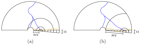
Figure 6. The cases (a) $s\alpha\leq(1-r)/2$ and (b) $s\alpha>(1-r)/2$ for the event $\mathcal{C}_{\pi+\alpha}^{2}(r,R)\setminus\mathcal{C}_{\pi}^{2}(r,R)$ in Proposition 3.6.

Finally, to show that $\delta_{0}$ may be taken to be independent of $r$ and $R$, we apply a multiplicative argument. Let $K>0$ be large enough and $\delta_{0}$ small enough that $P^{\delta}(\mathcal{C}_{\pi}^{2}(r,R))<(1/K)^{1-\epsilon}$ for all $0<\delta<\delta_{0}$. Insert concentric arcs of radii $r,rK,rK^{2},\ldots,rK^{\lfloor\log_{K}(R/r)\rfloor}$ between the arcs of radii $r$ and $R$, and consider the regions between successive pairs of these arcs. Since a crossing from the arcs of radius $r$ to the arc of radius $R$ implies that each of these regions is crossed, we have

$$P^{\delta}(\mathcal{C}^{2}_{\pi+\alpha}(r,R)) \leq\prod_{k=1}^{\lfloor\log_{K}(R/r)\rfloor}P^{\delta}\left(\mathcal{C}_{\pi+\alpha}^{2}\left(rK^{k},rK^{k+1}\right)\right)$$

$$\leq C\left(\frac{r}{R}\right)^{1-\epsilon}.\qed$$

Remark 3.7.

In particular, by taking $r=\delta$, the previous results yields bounds for half-disk crossing probabilities for $z\in\partial\Omega$.

Using Smirnov’s theorem, we can generalize one-arm estimates to annulus sectors of any angle.

Proposition 3.8.

For every $\epsilon>0$,

(3.8) $$P^{\delta}(\mathcal{C}_{\theta}^{1}(r,R))\lesssim\left(\frac{r}{R}\right)^{\frac{1}{3\theta}-\epsilon}.$$

Proof.

Smirnov’s theorem implies that for all $r$ and $R$ there exists $\delta_{0}=\delta_{0}(r,R,\epsilon)>0$ so that for all $0<\delta<\delta_{0}$, we have $P^{\delta}(\mathcal{C}_{\theta}^{1}(r,R))\leq(r/R)^{1/3\theta-\epsilon}$. As in the previous proposition, we can remove the dependence on $r$ and $R$ with a multiplicative argument. ∎

We can generalize the previous results for annular regions to a neighborhood of a meeting point of two analytic arcs. We let $\mathcal{C}_{\Omega,z}^{k}(r,R)$ denote the event that there exist $k$ disjoint crossings of alternating color contained in $\Omega$ and connecting the circles of radius $r$ and $R$ centered at $z$. We have the following corollary of Propositions 3.6 and 3.8.

Corollary 3.9.

Let $\epsilon>0$, let $\alpha=\alpha(\epsilon)$ be an angle satisfying the conclusion in Proposition 3.6. Let $\Omega$ be a piecewise analytic Jordan domain in $\mathbb{R}^{2}$. Fix $z\in\partial\Omega$ and suppose that $z$ is not a corner of $\Omega$. Let $R_{0}=R_{0}(z,\epsilon)>0$ be sufficiently small that $B_{R_{0}}(z)\cap\Omega$ is contained in a sector centered at $z$ and having angle $\pi+\alpha$ and radius $R_{0}$. Then for all $k\in\{1,2,3\}$ and for all $0<r<R\leq R_{0}$,

(3.9) $$P^{\delta}(\mathcal{C}^{k}_{\Omega,z}(r,R))\lesssim\left(\frac{r}{R}\right)^{k(k+1)/6-\epsilon},$$

with implied constants depending only on $\epsilon$.

Proof.

Since the event $\mathcal{C}^{k}_{\Omega}(r,R)$ implies a crossing of a sector of angle $\pi+\alpha$ with inner and outer radii of $r$ and $R$,

$$P^{\delta}(\mathcal{C}^{k}_{\Omega}(r,R))\leq P^{\delta}(\mathcal{C}_{\pi+\alpha}^{k}(r,R))$$

and we can estimate the probability on the right by Proposition 3.6 for $k\in\{2,3\}$ or Proposition 3.8 for $k=1$. ∎

We conclude this section by recording a generalization of the previous corollary for corners $z\in\partial\Omega$. The proof of this proposition uses convergence of the exploration path to $\mbox{SLE}_{6}$. We know how to remove this dependence on SLE results only when $k=1$, where Smirnov’s theorem suffices. We use (3.10) when $k\in\{2,3\}$ only to handle the case where $\Omega$ has reflex angles and to obtain the sharp exponent discussed in Remark 2.2.

Proposition 3.10.

Suppose that $z\in\partial\Omega$ is a corner of $\Omega$, but otherwise the hypotheses and variable definitions are the same as in Corollary 3.9. Then the conclusion holds, with (3.9) replaced by

(3.10) $$P^{\delta}(\mathcal{C}_{\Omega,z}^{k}(r,R))\lesssim\left(\frac{r}{R}\right)^{k(k+1)/12\theta-\epsilon},$$

where $2\pi\theta$ is the angle formed by $\partial\Omega$ at $z$.

Proof.

Define $a_{k,\delta}^{\theta}(r,R)$ to be the probability of $k$ disjoint crossings of alternating color from inner to outer radius in $\{z\,:\,\arg z\in(0,2\pi\theta)\text{ and }r<|z|<R\}$. In [SW01], it is shown that

(3.11) $$\lim_{\delta\to 0}a_{k,\delta}^{1/2}(1,R)=R^{-k(k+1)/6+o(1)},$$

using the convergence of the percolation exploration path to $\mbox{SLE}_{6}$. By the invariance of the law of $\mbox{SLE}_{6}$ under the conformal map $z\mapsto z^{2\theta}$, we conclude that (3.11) generalizes to

$$\lim_{\delta\to 0}a_{k,\delta}^{\theta}(1,R)=R^{-k(k+1)/12\theta+o(1)}.$$

The following multiplicative property is also used in [SW01]: for all $k<r\leq r^{\prime}\leq r^{\prime\prime}$, we have

(3.12) $$a^{1/2}_{k,\delta}(r,r^{\prime\prime})\leq a^{1/2}_{k,\delta}(r,r^{\prime})a^{1/2}_{k,\delta}(r^{\prime},r^{\prime\prime}).$$

This inequality still holds with $1/2$ replaced by $\theta$. The proof in [SW01] for the case $\theta=1/2$ relies only on these two facts and therefore generalizes to (3.10) for the sector domain $\{z\,:\,\arg z\in(0,2\pi\theta)\}$. The extension of this result to piecewise real-analytic Jordan domains with positive interior angles is obtained by following the same argument carried out in Corollary 3.9 for $\theta=1/2$. ∎

4. Proof of Main Theorem

4.1. Background and set-up

We begin by recalling few definitions and facts from complex analysis and differential geometry. See [A66], [Sil86], and [L03] for more details. If $a,b\in\mathbb{C}$ are linearly independent over $\mathbb{R}$ and $P$ is a parallelogram with vertex set $\{0,a,b,a+b\}$, then a function $f:P\to\mathbb{C}\cup\{\infty\}$ is said to be doubly-periodic if $f(z+a)=f(z)$ for $z$ on the segment from 0 to $b$ and $f(z+b)=f(z)$ for all $z$ on the segment from 0 to $a$. If $f$ is continuous, then such a function may be extended by periodicity to a continuous function defined on $\mathbb{C}$. An elliptic function is a doubly-periodic function whose extension to $\mathbb{C}$ is analytic outside of a set of isolated poles. Given distinct points $p_{1},p_{2}\in P$, there exists an elliptic function $f$ with simple poles at $p_{1},p_{2}$ (and no other poles) [Sil86, Proposition 3.4]. One way to obtain such a function is to define the Weierstrass product

$$\sigma(\zeta)=\zeta\prod_{\begin{subarray}{c}(j,k)\in\mathbb{Z}^{2}\\ (j,k)\neq(0,0)\end{subarray}}\left(1-\frac{\zeta}{aj+bk}\right)\exp\left(\frac{\zeta}{aj+bk}+\frac{\zeta^{2}}{2(aj+bk)^{2}}\right)$$

and set

(4.1) $$f(\zeta)=\frac{\sigma((\zeta-(p_{1}+p_{2})/2))^{2}}{\sigma(\zeta-p_{1})\sigma(\zeta-p_{2}).}$$

We recall the definitions of the differential forms $d\zeta=dx+i\,dy$ and $d\overline{\zeta}=dx-i\,dy$. Note that $d\bar{\zeta}\wedge d\zeta=2idA$, where $dA$ is the two-dimensional area measure and $\wedge$ is the usual wedge product. Recall that the exterior derivative $d$ maps $k$-forms to $(k+1)$-forms and satisfies

(4.2) $$df=\partial f\,d\zeta+\bar{\partial}fd\bar{\zeta},\text{ and }d(fd\zeta)=df\wedge d\zeta$$

for all smooth functions $f$.

Let $\phi:(\Omega,x(1),x(\tau),x(\tau^{2}))\to(T,1,\tau,\tau^{2})$ be the unique conformal map from $\Omega$ to the equilateral triangle $T$ with vertices $1,\tau,$ and $\tau^{2}$ which maps $x(\tau^{k})$ to $\tau^{k}$ for $k\in\{0,1,2\}$. Let $\delta>0$ be small and define $\Omega_{\text{edge}}$ to be such that $\Omega\setminus\Omega_{\text{edge}}$ is the set of all hexagonal faces of $(\Omega_{\delta})^{*}$ completely contained in $\Omega$. Let $T_{\text{edge}}$ be the image of $\Omega_{\text{edge}}$ under $\phi$.

We modify $G^{\delta}$ to obtain a function $\tilde{G}^{\delta}$ for which the lattice points on the boundary of $\Omega\setminus\Omega_{\text{edge}}$ are mapped to the boundary of $T$. Specifically, we set

$$\tilde{G}^{\delta}(z)=\begin{cases}\tau^{k}&z\text{ is adjacent to }x(\tau^{k})\\ \mathop{\rm proj}\nolimits\left(G^{\delta}(z),[\tau^{k},\tau^{k+1}]\right)&\text{if }z\text{ is not adjacent to }x(\tau^{k})\\ &\text{\hskip 28.45274ptbut is adjacent to }[x(\tau^{k+1}),x(\tau^{k+2})]\\ G^{\delta}(z)&\text{otherwise,}\end{cases}$$

where we are using the notation $\mathop{\rm proj}\nolimits(z,L)$ for the projection of a complex number $z$ onto the line $L\subset\mathbb{C}$. Now linearly interpolate to extend $\tilde{G}^{\delta}$ to a function on $\Omega$, and define $J:T\to T$ by $J(w)=\tilde{G}^{\delta}(\phi^{-1}(w))$.

Schwarz-reflect 17 times to extend $J$ to the parallelogram $P$ in Figure 8. For example, if $r$ is the reflection across the line through $1$ and $\tau$, then for $w$ in the triangle $r(T)$, we define $J(w)=r\circ J\circ r(w)$. Define an elliptic function $g_{w}$ via (4.1) with period parallelogram $P$ and poles at $p_{1}=w_{0}\colonequals(1+\tau+\tau^{2})/3$ and $p_{2}=w$ varying over the grey triangle $K$ in Figure 8.

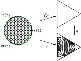
Figure 7. The function $J$ is defined as the composition of $\tilde{G}^{\delta}$ with the inverse of the Riemann map from $\Omega$ to the triangle. The region $T_{\text{edge}}$ is the image under the conformal map $\phi$ from $\Omega$ to $T$ of the region $\Omega_{\text{edge}}$, shown in green.

We will also need a result from the theory of Sobolev spaces. If $U\subset\mathbb{R}^{2}$ is a bounded domain, and $1\leq p<\infty$, we define the Sobolev space $W^{1,p}(U)$ to be the set of all functions $u:U\to\mathbb{R}$ such that the weak partial derivatives of $u$, $\frac{\partial u}{\partial x}$, and $\frac{\partial u}{\partial y}$ are in $L^{p}(U)$; see [E98] for more details. We equip $W^{1,p}(U)$ with the norm

$$\|u\|_{W^{1,p}}\colonequals\left\|u\right\|_{L^{p}(U)}+\left\|\frac{\partial u}{\partial x}\right\|_{L^{p}(U)}+\left\|\frac{\partial u}{\partial y}\right\|_{L^{p}(U)}.$$

Denote by $\operatorname{id}$ the identity function from $P$ to $P$, and define $C^{\infty}(P)$ to be the set of smooth, real-valued functions from $P$. Since $J$ is piecewise-affine on $P$, the real and imaginary parts of $J$ are in $W^{1,1}(P)$. Since $J$ is defined so that $J:T\to T$ takes vertices to vertices and boundary segments to boundary segments, $J-\operatorname{id}$ is continuous and doubly-periodic. Since smooth functions are dense in $W^{1,1}(P)$ and $L^{\infty}(P)$ [E98], for each $\epsilon>0$ we obtain a pair of smooth functions $Q_{1},Q_{2}\in C^{\infty}(P)$ such that

$$|Q(w)-(J(w)-w)| <\epsilon\text{ for all }w\in P,$$

(4.3) $$\|Q_{1}-\mathop{\rm Re}\nolimits(J-\text{id})\|_{W^{1,1}} <\epsilon,\text{ and}$$

$$\|Q_{2}-\mathop{\rm Im}\nolimits(J-\text{id})\|_{W^{1,1}} <\epsilon,$$

where $Q=Q_{1}+iQ_{2}$ (for see [E98] §5.3.3 and §C.5, for example). Defining $Q_{1}$ and $Q_{2}$ to be bump function convolutions, we arrange for $Q_{1}$ and $Q_{2}$ to inherit periodicity from $J-\operatorname{id}$. We note that by choosing $\epsilon$ sufficiently small in (4.3), we can for every $\epsilon^{\prime}>0$ choose $Q$ so that

(4.4) $$\int_{P}\left|\partial Q-\partial(J-\operatorname{id})\right|\left|g_{w}\right|\,dA<\epsilon^{\prime},$$

where $dA$ refers to two-dimensional Lebesgue measure. One way to see this is to define $f(z)=\partial Q(z)-\partial(J(z)-z)$ and note that for $R>0$, we have

(4.5) $$\|fg\|_{L^{1}} \leq R\|f\|_{L^{1}}+\|f\|_{L^{\infty}}\|\mathbf{1}_{\{|g|>R\}}g\|_{L^{1}}.$$

By the dominated convergence theorem, we may choose $R$ sufficiently large that the second term on the right-hand side is less than $\epsilon^{\prime}/2$. Once $R$ is chosen, we may choose $Q$ so that $\|f\|_{L_{1}}\leq\epsilon^{\prime}/(2R)$, by (4.3). Then (4.4) follows from (4.5).

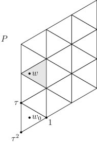
Figure 8. We extend $J(w)$ to a function on the parallelogram $P$, which is a union of 18 small triangles. The elliptic function $g_{w}:P\to\hat{\mathbb{C}}$ has poles at $w_{0}$ fixed and $w$ varying in the gray region.

4.2. Proof of main theorems

Proof of Theorem 2.1.

The following calculation is similar to the proof of the Cauchy integral formula, but with two key changes: we keep track of the $\bar{\partial}$ term, and we use the elliptic function $g_{w}$ in place of the usual kernel $\zeta\mapsto 1/\zeta$. Choose $r>0$ sufficiently small that the balls $B_{1}$ and $B_{2}$ of radius $r$ around $w_{0}$ and $w$ are disjoint, and apply Stokes’ theorem to the region $P\setminus(B_{1}\cup B_{2})$ to obtain that for smooth, complex-valued, periodic functions $Q$ on $P$, we have

$$-\int_{|\zeta-w|=r}Q(\zeta)g_{w}(\zeta)\,d\zeta- \int_{|\zeta-w_{0}|=r}Q(\zeta)g_{w}(\zeta)\,d\zeta=\int_{P\setminus(B_{1}\cup B_{2})}d(Qg_{w}d\zeta).$$

Note that the integral around $\partial\Omega$ vanishes by periodicity. Applying (4.2) and the product rule, we obtain

$$\int_{P\setminus(B_{1}\cup B_{2})}d(Qg_{w}d\zeta) =\int_{P\setminus(B_{1}\cup B_{2})}\left[\rule[-6.0pt]{0.0pt}{6.0pt}(\partial Qd\zeta+\bar{\partial}Qd\bar{\zeta})g_{w}+(\partial g_{w}d\zeta+\bar{\partial}g_{w}d\bar{\zeta})Q\right]\wedge d\zeta$$

$$=\int_{P\setminus(B_{1}\cup B_{2})}\bar{\partial}Q(\zeta)g_{w}(\zeta)\,d\bar{\zeta}\wedge d\zeta.$$

Let $Q$ be a smooth, complex-valued, periodic function on $P$ such that (4.3) and (4.4) are satisfied with $\epsilon=\epsilon^{\prime}=\delta^{100}$, say. Since $Q$ is bounded and $g$ has an integrable pole at $\zeta$, we can take $r\to 0$ and apply the dominated convergence theorem. We obtain

(4.6) $$2\pi iQ(w)\mathop{\rm Res}(g_{w},w)+2\pi iQ(w_{0})\mathop{\rm Res}(g_{w},w_{0})=2i\int_{P}\bar{\partial}Q(\zeta)g_{w}(\zeta)\,dA(\zeta),$$

where $dA(\zeta)=dx\,dy$ is notation for the area differential. The key step of the proof is to bound the right-hand side of (4.6) by $O(\delta^{c})$. To do this, we first consider $J$ in place of $Q$, and we estimate the integral over the regions $T\setminus T_{\text{edge}}$ and $T_{\text{edge}}$ separately. We postpone the details of these calculations to the following section, along with stronger lemma statements (Lemmas 5.2 and 5.4).

Lemma 4.1.

There exists $c>0$ so that

(4.7) $$\int_{T_{\text{edge}}}\bar{\partial}J(\zeta)g_{w}(\zeta)dA(\zeta)=O(\delta^{c}),$$

where the implied constants depend only on the three-pointed domain.

Lemma 4.2.

There exists $c>0$ so that

(4.8) $$\int_{T\setminus T_{\text{edge}}}\bar{\partial}J(\zeta)g_{w}(\zeta)dA(\zeta)=O(\delta^{c}),$$

where the implied constants depend only on the three-pointed domain.

Since $\mathop{\rm Res}(g_{w},w)$ is a continuous function of $w$ with no zeros in $K$, there exists $C>0$ such that

$$0<C^{-1}<\mathop{\rm Res}(g_{w},w)<C<\infty,\qquad\forall w\in K,$$

and similarly for the residue at $w_{0}$. Therefore, (4.8) implies that $Q(w)$ is within $O(\delta^{c})$ of a constant function, as $w$ ranges over the gray triangle shown in Figure 8. By considering $w$ to be one of the vertices of the gray triangle (so that $J(w)-w=0$), we see that this constant function is $O(\delta^{c})$. We conclude that $Q(w)=O(\delta^{c})$. By (4.3), this implies $J(w)-w=O(\delta^{c})$. By definition, this is equivalent to $\tilde{G}^{\delta}(z)-\phi(z)=O(\delta^{c})$. The theorem follows, since $\tilde{G}^{\delta}$ agrees with $G^{\delta}$ except on the outermost layer of lattice points. ∎

We combine the rate of convergence for $H_{1}+\tau H_{\tau}+\tau^{2}H_{\tau^{2}}$ with the rate of convergence for $H_{1}+H_{\tau}+H_{\tau^{2}}$ near $\partial\Omega$ to prove the rate of convergence of the crossing probabilities.

Proof of Theorem 1.1.

Let $z\in[x(1),x(\tau)]$. First we note that $H^{\delta}_{\tau^{2}}(z)=O(\delta^{c})$ by Proposition 3.4. Hence, by Theorem 2.1,

$$H^{\delta}_{1}(z)+\tau H^{\delta}_{\tau}(z) =\phi(z)+O(\delta^{c})\,.$$

We also have that

$$H^{\delta}_{1}(z)+H^{\delta}_{\tau}(z)=1+O(\delta^{c})\,,$$

since $S^{\delta}(z)=1+O(\delta^{c})$ by Proposition 3.4 (ii). Since the vectors $(1,1),(1,\tau)\in\mathbb{C}^{2}$ are linearly independent, this concludes the proof. ∎

5. Bounding the error integral

5.1. Piecewise analytic Jordan domains

In this section, we prove the two lemmas used in the proof of the main theorem. We often treat the conformal map $\phi(z)$ like a power of $z$ when $z$ is near a corner of the domain $\Omega$. To make this precise, we use the following theorem from the conformal map literature [L57].

Theorem 5.1.

If $\Omega$ is a Jordan domain part of whose boundary consists of two analytic arcs meeting at a positive angle $2\pi\alpha$ at the origin, and if $\phi:\Omega\to\mathbb{H}$ is a Riemann map sending 0 to 0, then there exists a neighborhood $B$ of the origin and continuous functions $\rho_{1},\rho_{2}:B\cap\overline{\Omega}\to\mathbb{C}$ and $\rho_{3},\rho_{4}:\phi(B\cap\overline{\Omega})\to\mathbb{C}$ for which

$$\phi(z) =z^{1/(2\alpha)}\rho_{1}(z),\qquad\phi^{\prime}(z)=z^{1/(2\alpha)-1}\rho_{2}(z),$$

$$\phi^{-1}(z) =z^{2\alpha}\rho_{3}(z),\text{ and}\qquad(\phi^{-1})^{\prime}(z)=z^{2\alpha-1}\rho_{4}(z)$$

and $\rho_{i}(0)\neq 0$ for $i\in\{1,2,3,4\}$.

We choose a collection $\mathcal{B}$ of disks covering the boundary of $\Omega$ as follows (see Figure 9). For each $z\in\partial\Omega$, choose a disk $B(z)$ centered at $z$ and small enough that the boundary arc (or arcs) containing $z$ admits a Taylor expansion in $B(z)$. If necessary, shrink $B(z)$ so that $\partial\Omega$ is well-approximated by its tangent (or tangents, if $z$ is a corner point) in $B(z)$, in the sense of Propositions 3.6 and 3.10. If necessary, shrink $B(z)$ once more to ensure that $\Omega\cap B(z)$ has one component. From this collection of open disks, extract a finite subcover $\mathcal{B}=(B_{j})_{j=1}^{p}$ of $\partial\Omega$ containing $\mathcal{B}_{\text{corners}}=\{B(z)\,:\,z\text{ is a corner point}\}$. Then $\mathcal{B}$ is an annular region whose interior has positive distance from $\partial\Omega$. Thus, for all sufficiently small $\delta$, $\mathcal{B}$ covers $\Omega_{\text{edge}}$. Note that this cover has been chosen in a manner which depends only on $\Omega$ and $\epsilon$, and in particular is independent of $\delta$.

Throughout our discussion, we permit the constants in statements involving asymptotic notation to depend only on the three-pointed domain. We also use $C$ to represent an arbitrary constant which depends only on the three-pointed domain. When working with the variable $\epsilon$, we will frequently relabel small constant multiples of $\epsilon$ as $\epsilon$ from one line to the next.

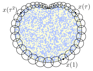
Figure 9. We cover the boundary with finitely many small disks, so that the boundary is approximately straight in each disk. Moreover, we ensure that every corner and every marked point is centered at one of these disks. More disks are required in regions of high curvature, as illustrated here for a domain bounded by a limaçon.

Lemma 5.2.

Let $J,g_{w}$ be as in Section 4, and suppose that the angle measures at marked points are $2\pi\alpha_{i}$ for $i=1,2,3$, and remaining angles are $2\pi\beta_{j}$ for $j=1,2,\ldots,n$. For every $\epsilon>0$,

(5.1) $$\int_{T_{\text{edge}}}\bar{\partial}J(\zeta)g_{w}(\zeta)dA(\zeta)\lesssim\delta^{\min_{i,j}\left(1,\frac{1}{6\alpha_{i}},\frac{1}{2\beta_{j}}\right)-\epsilon},$$

where the implied constants depend only on $\epsilon$ and the three-pointed domain.

Proof of Lemma..

Let $\mathcal{B}$ be as described above. Since the number of disks in $\mathcal{B}$ is bounded independently of $\delta$, it suffices to demonstrate that (5.1) holds for each one. Let $B\in\mathcal{B}$, and let $\pi\beta$ be the angle formed by $\partial\Omega$ center of $B$.

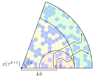
Figure 10. If $z$ is adjacent to the side $[x(\tau^{k+1}),x(\tau^{k+2})]$, then the distance from $G^{\delta}(z)$ to $\partial T$ is equal to the probability $H_{\tau^{k}}(z)$. This probability is bounded by that of a two-arm half-plane event with radius $k\delta$ and the two-arm $\beta$-annulus event with inner radius $2k\delta$ and constant-order outer radius.

To bound $\left|\int_{T_{\text{edge}}\cap\phi(\Omega\cap B)}\bar{\partial}J(\zeta)g_{w}(\zeta)dA(\zeta)\right|$, we index all the faces $\{F_{k}\}$ intersecting $\partial\Omega$ in such a way that the distance from $F_{k}$ to the center of $B$ is $\asymp k\delta$ for all $k$; this is possible since $\partial\Omega$ is piecewise smooth. We will bound the integral over each $F_{k}$ and then sum over $k$ (see Figure 10). Let $\zeta\in T_{\text{edge}}\cap\phi(F_{k})$ and suppose that $[\tau,\tau^{2}]$ is the closest boundary arc. We rewrite

(5.2) $$\bar{\partial}J(\zeta)=\bar{\partial}\tilde{G}^{\delta}(\phi^{-1}(\zeta))(\phi^{-1})^{\prime}(\zeta),$$

and we define $z=\phi^{-1}(\zeta)$. First we bound $\bar{\partial}\tilde{G}^{\delta}(z)$. In modifying $G^{\delta}(z)$ to obtain $\tilde{G}^{\delta}(z)$, the image of $z$ has to be moved no farther than $H_{1}(z)=\mathbb{P}(E_{1}(z))$, by the definition of $\tilde{G}^{\delta}(z)$. The event $E_{1}(z)$ entails a two-arm half-disk crossing and a two-arm $\beta$-annulus crossing (see Figure 10). Since these events occur in disjoint regions, they are independent and we can bound $\mathbb{P}(E_{1}(z))$ by the product of their probabilities. By Corollary 3.9, the two-arm half-plane exponent in $\Omega$, is 1 and by Proposition 3.10 the two-arm $\beta$-annulus exponent is $1/2\beta$. Thus the probability of $E_{1}(z)$ is at most $(k\delta)^{1/2\beta-\epsilon}(1/k)^{1-\epsilon}$. Hence for $z+\eta$ in the outermost layer and $z$ a neighbor of $z+\eta$, we have

$$\frac{1}{\delta} \left(\tilde{G}^{\delta}(z+\eta)-\tilde{G}^{\delta}(z)\right)$$

(5.3) $$=\frac{1}{\delta}\left(\tilde{G}^{\delta}(z+\eta)-G^{\delta}(z+\eta)+G^{\delta}(z+\eta)-G^{\delta}(z)+G^{\delta}(z)-\tilde{G}^{\delta}(z)\right)$$

$$\leq\frac{1}{\delta}\left((k\delta)^{1/2\beta-\epsilon}(1/k)^{1-\epsilon}+G^{\delta}(z+\eta)-G^{\delta}(z)\right).$$

$$\asymp\delta^{-1}(k\delta)^{1/2\beta-\epsilon}(1/k)^{1-\epsilon}.$$

In the last step we use a shifted domain trick (see the proof of the second inequality in Proposition 3.3 and Figure 5) and apply the trivial inequality $\mathbb{P}(A\setminus B)\leq\mathbb{P}(A)$. Using (5.3) to bound each term of the expression $\bar{\partial}\tilde{G}^{\delta}(z)=\left(\frac{\partial}{\partial\eta}\right.-\left.\frac{1}{\tau}\frac{\partial}{\partial(\tau\eta)}\right)\tilde{G}^{\delta}(z)$, we get $\bar{\partial}\tilde{G}^{\delta}(z)\asymp\delta^{-1}(k\delta)^{1/2\beta-\epsilon}(1/k)^{1-\epsilon}$.

We assume that the location $z$ of the pole is in the face nearest to the center of $B$ (since that is the worst case) and also that the image of the center of $B$ is not a vertex of the equilateral triangle $T$. We obtain

(5.4) $$\bigg{|}\int_{T_{\text{edge}}\cap\phi(\Omega\cap B_{j})} \bar{\partial}J(\zeta)g_{w}(\zeta)dA(\zeta)\bigg{|}$$

$$\leq\sum_{k=1}^{C/\delta}\sup_{z\in F_{k}}|\bar{\partial}\tilde{G}^{\delta}(z)(\phi^{-1})^{\prime}(\phi(z))g_{w}(\phi^{-1}(z))|\text{area}(\phi(F_{k}))$$

by replacing the integrand with its supremum on each $F_{k}$ and summing over $k$. We use the estimate $\text{area}(\phi(F_{k}))\lesssim\sup_{z\in F_{k}}|\phi^{\prime}(z)|^{2}\delta^{2}$ and use Theorem 5.1 to estimate the factors involving $\phi$. We bound the right-hand side of (5.4) by

$$\hskip 5.69046pt\lesssim\sum_{k=1}^{C/\delta}\overbrace{\delta^{-1}(k\delta)^{1/2\beta-\epsilon}(1/k)^{1-\epsilon}}^{\bar{\partial}\tilde{G}^{\delta}}\overbrace{(k\delta)^{1-1/2\beta}}^{(\phi^{-1})^{\prime}(\phi(z))}\overbrace{(k\delta)^{-1/2\beta}}^{g_{w}}\overbrace{\delta^{2}(k\delta)^{2/2\beta-2}}^{\text{area}(\phi(F_{k}))}$$

$$\hskip 5.69046pt\asymp\delta^{1-\epsilon}\left(\sum_{k=1}^{C/\delta}(k\delta)^{1/2\beta-2}\delta\right)$$

$$\hskip 5.69046pt\asymp\left\{\begin{array}[]{cl}\delta^{1-\epsilon}&\text{if }2\beta\leq 1\\ \delta^{1/2\beta-\epsilon}&\text{if }2\beta>1.\end{array}\right.$$

We have evaluated the sum by noting that the factor in parentheses is a convergent Riemann sum when the exponent is at least $-1$. When the exponent is less than $-1$, the summation over $k$ gives a constant factor, leaving the contributions of the powers of $\delta$.

If the center of $B_{j}$ is a marked point, the proof is essentially the same and the net effect is to replace $1/2\beta$ with $1/6\alpha$ throughout the calculation. These replacements are justified either by fewer percolation arms (when the exponent appears in an arm event estimate), or by the angle of $\pi/3$ at the vertices of the triangle $T$ (when the exponent appears because of the conformal map $\phi$). ∎

Remark 5.3.

We can remove the dependence on SLE by using Smirnov’s theorem to estimate one-arm $\beta$-annulus probabilities (instead of using Proposition 3.10). The result is that we obtain (5.1) with the right-hand side replaced by

$$\delta^{\min_{i,j}\left(1,\frac{1}{6\alpha_{i}},\frac{1}{6\beta_{j}}\right)-\epsilon}.$$

Lemma 5.4.

Let $J,g_{w},\{\alpha_{i}\},\{\beta_{j}\}$ be as in the statement of Lemma 5.2. Let $c_{3}=2/3$ be the 3-arm whole-plane exponent. Then

(5.6) $$\int_{T\setminus T_{\text{edge}}}\bar{\partial}J(\zeta)g_{w}(\zeta)dA(\zeta) \lesssim\delta^{\min_{i,j}\left(c_{3},\frac{1}{6\alpha_{i}},\frac{1}{2\beta_{j}}\right)-\epsilon},$$

where the implied constants depend only on $\epsilon$ and the three-pointed domain.

Proof of Lemma..

We will use Proposition 3.3 to bound $\bar{\partial}G$. Let $\mathcal{B}$ be as above and note that $\text{dist}(\partial\Omega,\Omega\setminus\bigcup\mathcal{B})>0$ by the discussion preceding Lemma 5.2.

We first handle $\Omega\setminus\bigcup\mathcal{B}$. Suppose that one of the five-arm events of Figure 5 occurs, say $E_{1,1,1}^{\text{five arm}}(z)$. Let $b$ be the point nearest $x(\tau^{2})$ where a blue arm touches down in the shifted domain, and let $s$ be the number of lattice units along the boundary from $b$ to $x(\tau^{2})$. When $z\notin\bigcup\mathcal{B}$ (see Figure 11), $z$ is well away from the boundary thus we note that such a five arm event entails the existence of:

1. a $3$-arm whole-plane event in alternating colors at $z$, in a ball of radius $\Theta(1)$,

2. a $3$-arm half-annulus event of alternating colors originating at $b$, in a semi-circle of radius $s\delta/2$, and

3. a $2$-arm half-annulus event in an annulus of inner radius $s\delta/2$ and outer radius $\Theta(1)$.

Since the derivative of the conformal map is bounded above and below for $z$ away from the boundary, we can ignore the contribution of $\phi^{\prime}(\phi^{-1}(z))$ in (5.2) and calculate

$$|\bar{\partial}J(z)| \lesssim\delta^{-1}\sum_{s=1}^{C/\delta}\overbrace{(\delta^{c_{3}-\epsilon})}^{\text{3-arm whole-plane}}\times\overbrace{(1/s)^{2}}^{\text{3-arm half-plane}}\times\overbrace{(s\delta)}^{\text{2-arm half-ann.}}$$

$$\lesssim\delta^{c_{3}-\epsilon}.$$

Hence we have

$$\left|\int_{\phi(\Omega\setminus\mathcal{B})}\bar{\partial}J(\zeta)g_{w}(\zeta)dA(\zeta)\right|\lesssim\delta^{c_{3}-\epsilon}\int_{\phi(\Omega\setminus\mathcal{B})}|g_{w}(\zeta)|\,dA(\zeta)\lesssim\delta^{c_{3}-\epsilon},$$

since a simple pole is integrable with respect to area measure.

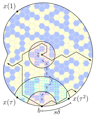
Figure 11. To bound the probability of the five-arm difference event described in Proposition 3.3, we consider three regions which contain two-arm or three-arm crossing events (these regions are shown in green and red, respectively).

To bound the integral of the union of the balls in $\mathcal{B}$, we handle each $B\in\mathcal{B}$ separately. We first consider a ball centered at a marked corner, say $x(\tau)$. Once again, for each $z$ and each percolation configuration, we define $b\in\partial\Omega$ to be the point nearest $x(\tau^{2})$ at which a blue arm from $z$ touches down in the shifted domain. This time we let $s$ be the graph distance from $b$ to the boundary point $z_{\text{foot}}$ nearest to $z$ (see Figure 14) and index the faces $F_{n,k}$ in such a way that if $z\in F_{n,k}$, $|x(\tau)-z|\asymp k\delta$ and $\operatorname{dist}(\partial\Omega,z)\asymp n\delta$. As above, we bound $|\bar{\partial}\tilde{G}^{\delta}(z)|$ using percolation arm estimates in each hexagonal face and sum over all the faces in $\phi(\Omega\cap B)$. By symmetry, it suffices to sum over only the faces which are closer to the boundary arc $[x(\tau),x(\tau^{2})]$ than to the boundary arc $[x(1),x(\tau)]$.

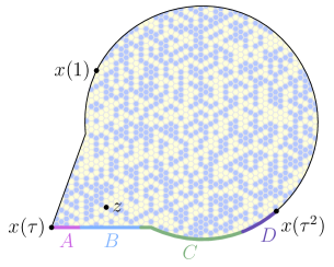
Figure 12. We sum over the possible locations for $b$, considering the cases $b\in A$, $b\in B$, $b\in C$, and $b\in D$ separately.

Suppose that the corner at $B$ is one of the three marked points and has interior angle $\alpha\pi$. We bound $|\bar{\partial}\tilde{G}^{\delta}|$ by summing over all possible locations for $b$. We consider four cases:

• Case A: $b$ is closest to the corner at $x(\tau)$ (Figure 13(a)),

• Case B: $b$ is within $k/2$ units of $z_{\text{foot}}$ (Figure 13(b)),

• Case C: $b$ is more than $k/2$ units to the right of $z_{\text{foot}}$ but closer to $z_{\text{foot}}$ than to $x(\tau^{2})$ (Figure 13(c)), and

• Case D: $b$ is closest to $x(\tau^{2})$ (Figure 13(d)).

For simplicity, we assume that $[x(\tau),x(\tau^{2})]$ is a real analytic arc (that is, that there are no corners between $x(\tau)$ and $x(\tau^{2})$). It will be apparent that similar estimates hold when additional corners are accounted for.

Denote by $P(z,b)$ the contribution to $\bar{\partial}G^{\delta}$ of the five-arm event with missed connection at $b$ (see Figure 5). As in (5.4), we bound the sum for Case A by a constant times

$$\sum_{k=1}^{C/\delta}\sum_{n=1}^{Ck}\sum_{r=1}^{k/2} \overbrace{\underbrace{\delta^{-1}}_{\bar{\partial}}\underbrace{n^{-c_{3}-\epsilon}}_{\text{3-arm disk.}}\underbrace{r^{-2}}_{\text{3-arm half-disk.}}\underbrace{\left(\frac{r}{k}\right)^{1/2\alpha-\epsilon}}_{\text{2-arm }\alpha\text{-ann.}}\underbrace{(k\delta)^{1/6\alpha-\epsilon}}_{\text{1-arm }\alpha\text{-ann.}}}^{P(z,b)}$$

$$\hskip 85.35826pt\times\overbrace{(k\delta)^{1-1/6\alpha}}^{(\phi^{-1})^{\prime}(\phi(F_{n,k}))}\overbrace{\delta^{2}(k\delta)^{1/3\alpha-2}}^{\text{area}(\phi(F_{n,k})))}\overbrace{(k\delta)^{-1/6\alpha}}^{g_{w}}$$

$$\lesssim\delta^{\min(c_{3},1/6\alpha)-\epsilon}.$$

We upper bound the contribution of Case B by a constant times

$$\sum_{k=1}^{C/\delta}\sum_{n=1}^{Ck}\sum_{s=1}^{k/2} \overbrace{\underbrace{\delta^{-1}}_{\bar{\partial}}\underbrace{n^{-c_{3}-\epsilon}}_{\text{3-arm disk}}\underbrace{\frac{1}{s^{2}+n^{2}}}_{\text{3-arm half disk}}\underbrace{\frac{\sqrt{s^{2}+n^{2}}}{k}}_{\text{2-arm half-ann.}}\underbrace{(k\delta)^{1/6\alpha-\epsilon}}_{\text{1-arm }\alpha\text{-ann.}}}^{P(z,b)}$$

$$\hskip 85.35826pt\times\overbrace{(k\delta)^{1-1/6\alpha}}^{(\phi^{-1})^{\prime}(\phi(F_{n,k}))}\overbrace{\delta^{2}(k\delta)^{1/3\alpha-2}}^{\text{area}(\phi(F_{n,k}))}\overbrace{(k\delta)^{-1/6\alpha}}^{g_{w}}$$

$$\lesssim\delta^{\min(c_{3},1/6\alpha)-\epsilon}.$$

For Case C, we get

$$\sum_{k=1}^{C/\delta}\sum_{n=1}^{Ck}\sum_{r=k/2}^{C/\delta} \overbrace{\underbrace{\delta^{-1}}_{\bar{\partial}}\underbrace{n^{-c_{3}-\epsilon}}_{\text{3-arm disk.}}\underbrace{k^{-2}}_{\text{3-arm half-disk.}}}^{P(z,b)}(k\delta)^{1-1/6\alpha}\delta^{2}(k\delta)^{1/3\alpha-2}(k\delta)^{-1/6\alpha}$$

$$\lesssim\delta^{1/6\alpha-\epsilon}.$$

For Case D, we denote by $2\pi\gamma$ the angle at $x(\tau^{2})$ and by $t$ the number of lattice units from $x(\tau^{2})$ to $b$. We obtain

$$\sum_{k=1}^{C/\delta}\sum_{n=1}^{Ck}\sum_{t=1}^{C/\delta} \overbrace{\underbrace{\delta^{-1}}_{\bar{\partial}}\underbrace{n^{-c_{3}-\epsilon}}_{\text{3-arm disk.}}\underbrace{t^{-2}}_{\text{3-arm half-disk.}}\underbrace{(t\delta)^{1/\gamma}}_{\text{2-arm }\gamma\text{ ann}}}^{P(z,b)}(k\delta)^{1-1/6\gamma}\delta^{2}(k\delta)^{1/3\gamma-2}(k\delta)^{-1/6\gamma}$$

$$\lesssim\delta^{1/2\gamma-\epsilon}.$$

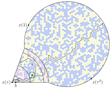
(a)

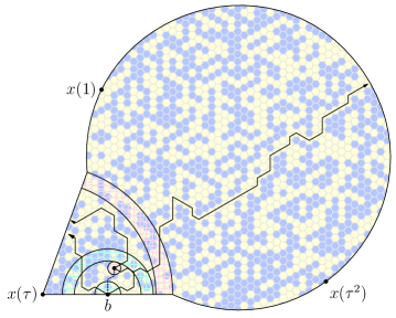
(b)

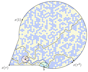
(c)

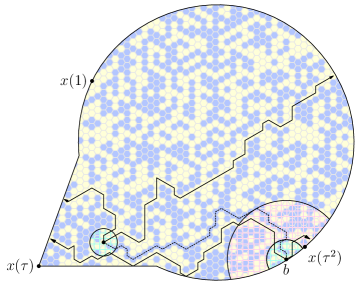
(d)

Figure 13. Assuming that $z$ is near a marked corner, we have four cases to consider: (a) $b$ is close to $x(\tau)$, (b) $b$ is close to $z$, (c) $b$ is between $z$ and $x(\tau^{2})$ but far from both, and (d) $b$ is close to $x(\tau^{2})$. For a closer view of the corner with additional labels, see Figure 14.

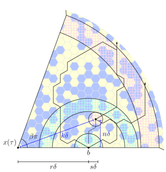
Figure 14. A close-up view of the corner of Figure 13(b), with labels illustrating the roles of $k$, $n$, $r$, and $s$. The faces are indexeed by $k$ and $n$ in such a way that the distance from $z$ to the corner is $\asymp k\delta$ and the distance from $z$ to $\partial\Omega$ is $\asymp n\delta$. Similarly, the faces intersecting the boundary are indexed so that the distance along the boundary from the corner to $b$ is $\asymp r\delta$ and the distance from $b$ to $z_{\text{foot}}$ is $\asymp s\delta$.

The proofs for the bounds in a disk whose center is not marked are essentially the same as these. As in the proof of Lemma 5.2, the net effect is to replace $1/6\alpha$ with $1/2\beta$. ∎

Remark 5.5.

As in Remark 5.3, we can remove the dependence on SLE by using Smirnov’s theorem instead of Proposition 3.10, under the additional assumption that $\partial\Omega$ has no reflex angles (that is, $\max_{i,j}(\alpha_{i},\beta_{j})\leq 1/2$). By using the weaker one-arm $\beta$-annulus bound in place of the two-arm and three-arm bounds, we obtain (5.6) with the right-hand side replaced by

$$\delta^{\min_{i,j}\left(c_{3},\frac{1}{6\alpha_{i}},\frac{1}{6\beta_{j}}\right)-\epsilon}.$$

Without the help of SLE, our techniques break down in the presence of reflex angles.

5.2. Uniform bounds for half-annulus domains

While the constants in Theorem 1.1 generally depend on the three-pointed domain, there are some classes of domains for which Theorem 1.1 holds with uniform constants. In preparation for the proof of Theorem 1.2, we obtain uniform constants for a class of half-annulus domains with arbitrarily small ratio of inner to outer radius.

Let $\Omega_{r,R}\subset\mathbb{H}$ be the origin-centered half-annulus of inner and outer radius $r$ and $R$, respectively. Let $T_{\text{unit}}$ be the triangle with vertices $0,1,$ and $e^{i\pi/3}$, and define $\phi_{r,R}:\Omega_{r,R}\to T_{\text{unit}}$ to be the conformal map sending $-R$, $-r$, and $R$ to $e^{i\pi/3},0$, and $1$, respectively. For $r\geq 0$, define $S_{r}=\{re^{i\theta}\,:0\leq\theta\leq\pi\}$.

Proposition 5.6.

For all $0<c<c_{3}=2/3$ and $0<\delta\leq r\leq 1/2$, we have

(5.7) $$P^{\delta}(S_{r}\leftrightarrow S_{1})-\phi_{r,1}(r)=O(r^{-1/3}\delta^{c})=O(\delta^{c-1/3}),$$

where the implied constants depend only on $c$ and, in particular, are uniform over $r\in(0,1/2]$.

Remark 5.7.

To ensure that the interval $(0,c_{3}-1/3)$ of possible exponents $c$ is nonempty, we need the SLE result that the three-arm whole-plane exponent $c_{3}$ is greater than $1/3$.

Proof.

We proceed by modifying Lemmas 5.2 and 5.4 to prove (5.1) and (5.6) with constants uniform over the domains $\Omega_{r,1}$. For $z\in\mathbb{C}$ and $\rho\geq 0$, let $B(z,\rho)$ be the disk of radius $\rho$ centered at $z$. For the integral over $\Omega_{r,1}\setminus B(0,1/2)$ we obtain a bound of $O(\delta^{2/3-\epsilon})$ by Lemmas 5.2 and 5.4, so it suffices to consider the integral over $\Omega_{r,1}\cap B(0,1/2)$.

Fix $\epsilon>0$, and determine $\alpha(\epsilon)$ from Proposition 3.6. Choose $\eta(\epsilon)$ small enough that $B(i,\eta)\setminus B(0,1)$ is contained in a sector of angle $\pi+\alpha$ centered at $i$. Cover $S_{r}$ with finitely many balls of radius $2r\eta$ in such a way that $\bigcup_{w\in S_{r}}B(w,r\eta)$ is contained in the union $U$ of the balls. By Lemmas 5.2 and 5.4 and rescaling (5.1) and (5.6) by a factor of $r$, we find that $\int_{U}|\bar{\partial}Jg_{w}|\,dA=O(r^{-1/3}\delta^{c_{3}-\epsilon})$. So it remains to consider the integral over the annulus $A^{\prime}\colonequals\{z\,:\,r(1+\eta)<|z|<1/2\}$. We reduce further to considering the integral over the left half $\{z\in A^{\prime}:\pi/2<\text{arg}(z)<\pi\}$ of $A^{\prime}$, since the contribution from the right half of $A^{\prime}$ is smaller. We compute this integral similarly to those in Lemmas 5.2 and 5.4 (see Figure 15): we index the faces $F_{n,k}$ in such a way that $|F_{n,k}|-r\asymp k\delta$ and $\operatorname{dist}(F_{n,k},\mathbb{R})\asymp n\delta$ and, for $z\in F_{n,k}$ we bound

$$P(z,b)\lesssim$$

$$\underbrace{\delta^{-1}}_{\bar{\partial}}\underbrace{(n\wedge k)^{-c_{3}+\epsilon}}_{\text{3-arm disk.}}\underbrace{\left(\frac{\delta}{s\delta\wedge\eta r}\right)^{2-\epsilon}}_{\text{3-arm half-disk.}}\underbrace{\left(\frac{s\delta\wedge\eta r}{\eta r}\right)^{1-\epsilon}}_{\text{2-arm half ann.}}\underbrace{\left(\frac{r}{k\delta+r}\right)^{1-\epsilon}}_{\text{2-arm }\text{half-ann.}}\underbrace{(k\delta+r)^{1/3-\epsilon}}_{\text{1-arm }\text{half-ann`.}}.$$

Figure 16 shows how to write $\phi_{r,1}$ as a composition of simpler conformal maps. Using this composition, we compute

$$\phi_{r,1}(z) \asymp\frac{(z+r)^{2/3}}{z^{1/3}},$$

$$\phi_{r,1}^{\prime}(z) \asymp\frac{z-r}{z^{4/3}(z+r)^{1/3}},\text{ and}$$

$$\phi_{r,1}^{-1}(\phi_{r,1}(z)) \asymp\frac{z^{4/3}(z+r)^{1/3}}{z-r}.$$

Using these estimates, we can upper bound $\int|\bar{\partial}Jg_{w}|\,dA$ by summing over the faces $F_{n,k}$. We obtain

$$\sum_{k=\eta r/\delta}^{C/\delta}\sum_{n=1}^{Ck}\sum_{s=1}^{Cr/\delta} P(z,b)\overbrace{(k\delta+r)^{1/3}(k\delta)^{1/3}}^{(\phi^{-1})^{\prime}(\phi(F_{n,k}))}\overbrace{\delta^{2}(k\delta+r)^{-2/3}(k\delta)^{-2/3}}^{\text{area}(\phi(F_{n,k}))}\overbrace{\frac{(k\delta+r)^{1/3}}{(k\delta)^{2/3}}}^{g_{w}}$$

$$\lesssim r^{-1/3}\delta^{c_{3}-\epsilon}.$$

∎

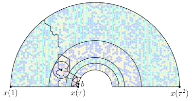
Figure 15. We use crossing events for the five regions shown to bound the probability of a five-arm event for which $b\in S_{r}$.

6. Half-plane exponent

We begin with a lemma about the conformal maps $\phi_{r,R}:\Omega_{r,R}\to T_{\text{unit}}$; see Subsection 5.2 for notation.

Lemma 6.1.

There exist $a_{1},a_{2}>0$ so that for all $r,R>0$ such that $r/R<1/2$, we have

(6.1) $$a_{1}\leq\frac{\phi_{r,R}(r)}{(r/R)^{1/3}}\leq a_{2}.$$

Proof.

By scaling, we may assume $R=1$. Consider the sequence of conformal maps illustrated in Figure 16. Let us call these maps $f_{n}$ for $n=1,2,\ldots,5$, so that $f_{n}:D_{n}\to D_{n+1}$. Since the domains are Jordan, we may regard $f_{n}$ as a continuous map defined on the closure of each domain. Define the compositions $\tilde{f}_{n}=f_{n}\circ f_{n-1}\cdots\circ f_{1}$.

For $n\geq 2$, let $K_{n}\subset D_{n}$ denote the image of

$$K_{1}\colonequals\{z\,:\,|z|=r\text{ and }\arg z\in[0,\pi/2]\}\cup[r,1/2]$$

under $\tilde{f}_{n-1}$. For $n\in\{2,3,5\}$, regard $f_{n}$ as having been analytically continued in a neighborhood of every straight boundary (by Schwarz reflection), and define $m_{n}$ and $M_{n}$ to be the infimum and supremum of $f_{n}^{\prime}(z)$ as $z$ ranges over $K_{n}$ and $r$ ranges over $[0,1/2]$.

We claim that $0<m_{n}<M_{n}<\infty$ for all $n\in\{2,3,5\}$. For $n=5$, this follows from the continuity of $f_{n}^{\prime}$ and the fact that the derivative of a conformal map cannot vanish. For $n=3$, this follows from the joint continuity of the Möbius map $(z-w)/(1-\overline{w}z)$ in $w$ and $z$.

The case $n=2$ requires more care, since the eccentricity of $D_{2}$ depends on $r$. We introduce the notation $D_{2,r}$ and $f_{2,r}$ to indicate this dependence. Let $I\subset(0,1/2)$ be an interval. We claim that for every fixed $z\in\bigcap_{r\in I}D_{2,r}$, the quantity $f_{2,r}^{\prime}(z)$ is continuous in $r$. We first recall some definitions from complex analysis: given a simply connected domain $U\subset\mathbb{C}$ and a point $z\in U$, we will say that a Riemann map $\varphi:\mathbb{D}\to U$ is normalized if $\varphi(0)=z$ and $\varphi^{\prime}(0)>0$. Recall that a sequence of open sets $U_{n}\subset\mathbb{C}$ converges to an open set $U\subset\mathbb{C}$ in the Carathéodory sense with respect to $z\in U$ if (a) for all compact $K\subset U$ containing $z$, we have $K\subset U_{n}$ for all $n$ sufficiently large, and (b) $U$ contains every open set satisfying condition (a). If $U_{n}\to U$ in the Carathéodory sense, then the normalized Riemann maps $\varphi_{n}:\mathbb{D}\to U_{n}$ converge uniformly on compact subsets to the normalized Riemann map $\varphi:\mathbb{D}\to U$ [Wen92]. Observe that if $r_{n}\to r$, $D_{2,r_{n}}$ converges to $D_{2,r}$ with respect to 0 in the Carathéodory sense. Hence $f_{2,r_{n}}\to f_{2,r}$ uniformly on compact sets, which in turn implies that $f^{\prime}_{2,r_{n}}\to f^{\prime}_{2,r}$ uniformly on compact sets. In particular, we obtain joint continuity of $f_{2,r}^{\prime}(z)$ in $z$ and $r$. It follows that the infimum and supremum of $|f_{r}^{\prime}(z)|$ over $(z,r)\in K_{n}\times[0,1/2]$ are achieved, which implies $0<m_{2}<M_{2}<\infty$.

Since $f_{1}(r)=2r/(1+r^{2})$, we have

$$r\leq f_{1}(r)\leq 2r.$$

We note that each $f_{n}$ is monotone on the real line, and apply $f_{5}\circ f_{4}\circ f_{3}\circ f_{2}$ to the inequality above. Using our derivative bounds, we obtain

$$m_{5}\left(m_{2}m_{3}r\right)^{1/3}\leq\tilde{f}_{4}(r)\leq M_{5}\left(2M_{2}M_{3}r\right)^{1/3},$$

thus the result holds with $a_{1}=m_{5}(m_{2}m_{3})^{1/3}$ and $a_{2}=M_{5}(2M_{2}M_{3})^{1/3}$. ∎

Remark 6.2.

Numerical evidence suggests that Lemma 6.1 holds with $a_{1}=1$ and $a_{2}\approx 1.426$.

We denote by $P$ the measure $P^{\delta=1}$ corresponding to site percolation on the triangular lattice with unit mesh size.

Lemma 6.3.

For all $0<c<c_{3}-1/3=1/3$ there exists $R_{0}>1$ such that for all $R\geq R_{0}$ and for all $r\leq\frac{1}{2}R$,

(6.2) $$\left|P^{\delta=1}(S_{r}\leftrightarrow S_{R})-\phi_{r,R}(r)\right|\leq\frac{a_{1}}{10}R^{-c}.$$

Proof.

This follows immediately from Proposition 5.6, by rescaling by a factor of $R$. Note that we have used the openness of interval $(0,c_{3}-1/3)$ to deal with the multiplicative constant in the bound given by Proposition 5.6. ∎

(a) Half-annulus $D_{1}$

(b) Half-ellipse $D_{2}$

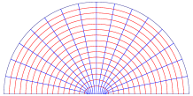
(c) Half-disk $D_{3}$

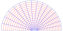
(d) Half-disk $D_{4}$

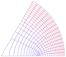
(e) Sector $D_{5}$

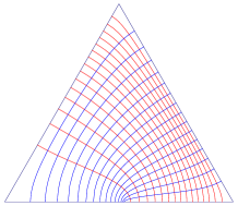
(f) Equilateral triangle $D_{6}$

Figure 16. Panels (b) through (f) show the images of the half-annulus in panel (a) under successive conformal maps. Composing these maps gives the conformal map $\phi_{r,R}$ from the half-annulus to the equilateral triangle which sends $-R$, $-r$, and $R$ to $e^{i\pi/3}$, 0, and 1. The ratio of outer radius to inner radius is 20 for the half-annulus shown. The map from $D_{1}$ to $D_{2}$ is a suitable scaling of $z\mapsto z+1/z$. The map from $D_{2}$ to $D_{3}$ is the restriction of the conformal map from an ellipse to the disk. From $D_{3}$ to $D_{4}$, a Möbius map moves the image of $-r$ to the origin. The map from $D_{4}$ to $D_{5}$ is the cube root, and the map from $D_{5}$ to $D_{6}$ is the restriction to a sector of the Schwarz-Christoffel map from the disk to the regular hexagon.

Proof of Theorem 1.2.

Let $\epsilon>0$, and define $R_{0}=e^{\sqrt{\log\log R}}$. We assume that $R$ is sufficiently large that $R_{0}$ satisfies the statement of Lemma 6.3. Define $\alpha=1/(1-3c)$ and $n=\lfloor\log_{R_{0}}\log_{\alpha}R\rfloor$. Let $R_{k}=R_{0}^{\alpha^{k}}$ for $1\leq k\leq n-1$, and let $R_{n}=R$. We first prove the upper bound. Since an open path from $0$ to $S_{R}$ includes a crossing from $S_{R_{k}}$ to $S_{R_{k+1}}$ for all $0\leq k<n$, we may use Lemma 6.1, Lemma 6.3, and independence to compute

$$P(0\leftrightarrow S_{R}) \leq\prod_{k=0}^{n-1}P(S_{R_{k}}\leftrightarrow S_{R_{k+1}})$$

$$\leq\prod_{k=0}^{n-1}\left[a_{2}\left(\frac{R_{k+1}}{R_{k}}\right)^{-1/3}+\frac{a_{1}}{10}R_{k+1}^{-c}\right],$$

by (6.2). Factoring out the first term in brackets and splitting the product, we obtain

$$P(0\leftrightarrow S_{R}) \leq\prod_{k=0}^{n-1}a_{2}\prod_{k=0}^{n-1}\left(\frac{R_{k+1}}{R_{k}}\right)^{-1/3}\prod_{k=0}^{n-1}\left[1+a_{1}(10a_{2})^{-1}R_{k+1}^{1/3-c}R_{k}^{-1/3}\right]$$

$$\leq(a_{1}/10+a_{2})^{n-1}(R/R_{0})^{-1/3},$$

because the second term in brackets simplifies to $a_{1}/(10a_{2})$ by our choice of $R_{k}$. Substituting the value of $n$ gives

$$P(0\leftrightarrow S_{R}) \leq R_{0}^{1/3}(\log\alpha)^{-\log(a_{1}/10+a_{2})/\log R_{0}}(\log R)^{\log(a_{1}/10+a_{2})/\log R_{0}}R^{-1/3}$$

$$\leq e^{C\sqrt{\log\log R}}R^{-1/3},$$

for some constant $C$ and for sufficiently large $R$, which gives the upper bound.

For the lower bound (see Figure 17), we define $R^{\prime}_{k}=2R_{k}$. Define $E_{k}$ to be the event that there is an open crossing of $\Omega_{R_{k},R_{k}^{\prime}}$ from $[R_{k},R_{k}^{\prime}]$ to $[-R_{k}^{\prime},-R_{k}]$. By the Russo-Seymour-Welsh inequality, this probability is bounded below by a constant $p$ which does not depend on $k$. Note that there is a path from the origin to $S_{R}$ if the following events occur:

1. there is an open path from the origin to $S_{R^{\prime}_{0}}$,

2. there is an open path from $S_{R_{k}}$ to $S_{R^{\prime}_{k+1}}$ for all $0\leq k<n$, and

3. $E_{k}$ occurs for all $0\leq k<n$.

Since these events are increasing, we can use the FKG inequality to lower bound the probability of their intersection by the product of their probabilities. We obtain

$$P(0\leftrightarrow S_{R}) \geq P(0\leftrightarrow S_{R_{0}})\prod_{k=0}^{n-1}P(S_{R_{k}}\leftrightarrow S_{R^{\prime}_{k+1}})\prod_{k=0}^{n-1}P(E_{k})$$

$$\geq R_{0}^{-1/2}p^{n-1}\prod_{k=0}^{n-1}\left[a_{1}\left(\frac{R_{k+1}^{\prime}}{R_{k}}\right)^{-1/3}-\frac{a_{1}}{10}(R^{\prime}_{k+1})^{-c}\right],$$

since $P(0\leftrightarrow S_{R_{0}})=R_{0}^{-1/3+o(1)}\gtrsim R_{0}^{-1/2}$, by the Cardy-Smirnov theorem. Factoring as before and simplifying, we obtain

$$P(0\leftrightarrow S_{R}) \geq R_{0}^{-1/2}(a_{1}p)^{n-1}\prod_{k=0}^{n-1}\left(\frac{R^{\prime}_{k+1}}{R_{k}}\right)^{-1/3}\prod_{k=0}^{n-1}\left[1-\frac{1}{10}(R^{\prime}_{k+1})^{1/3-c}R_{k}^{-1/3}\right]$$

$$\geq R_{0}^{-1/2}2^{-n/3}(a_{1}p)^{n-1}\prod_{k=0}^{n-1}\left(\frac{R_{k+1}}{R_{k}}\right)^{-1/3}\prod_{k=0}^{n-1}\left[1-\frac{2^{1/3-c}}{10}R_{k+1}^{1/3-c}R_{k}^{-1/3}\right]$$

$$\geq R_{0}^{-1/2}2^{-n/3}\left[a_{1}p(1-2^{1/3-c}/10)\right]^{n-1}(R/R_{0})^{-1/3}$$

$$\geq e^{-C\sqrt{\log\log R}}R^{-1/3},$$

for some constant $C>0$ and sufficiently large $R$. ∎

Figure 17. If there are segment-to-segment crossings of each narrow half-annulus, crossings from $S_{R_{k}}$ to $S_{R_{k}^{\prime}}$ for each $0\leq k\leq n$, and an open path from the origin to $S_{R_{0}}$, then there is an open path from the origin to $S_{R}$. The figure shown is an image under radial logarithmic scaling $(r,\theta)\mapsto(\log r,\theta)$.

References

- [A66] Alfors, L. Complex Analysis. McGraw-Hill Book Company, Inc., New York, 1966
- [B07] Beffara, V. Cardy’s formula the easy way. http://www.umpa.ens-lyon.fr/vbeffara/files/Proceedings-Toronto.pdf, 2007
- [BCL12] Binder, I., Chayes L., and Lei H.K. On the Rate of Convergence for Critical Crossing Probabilities, Ann. Inst. Henri Poincaré, to appear, 2013.
- [CN07] Camia, F. and Newman, C. M. Critical percolation exploration path and SLE6: a proof of convergence. Probab. Theory Related Fields, 139:473–519, 2007
- [CS12] Chelkak, D. and Smirnov, S. Universality in the 2D Ising model and conformal invariance of fermionic observables, Inv. Math. 189, 515-580, 2012
- [DS12] Duminil-Copin, H., and Smirnov, S. Conformal invariance of lattice models, Lecture notes (Clay Summer School 2010), arXiv:math/0108211v1.
- [E98] Evans, L. C., Partial Differential Equations, Graduate Studies in Mathematics, ISBN 0-821-80772-2, American Mathematical Society, 1998
- [HS12] Hongler, C. and Smirnov, S. The energy density in the planar Ising model, Acta Math., to appear.
- [KN] Kozma, G. and Nachmias, A. The halfplane exponent above the critical dimension, in preparation.
- [L03] Lee, J. Introduction to Smooth Manifolds, Graduate Texts in Mathematics, Springer-Verlag, New York, 2003
- [L57] Lehman, S. Development of the mapping function at an analytic corner. Pacific J. Math. Volume 7, Number 3, 1437-1449, 1957
- [LSW01] Lawler, G., Schramm, O., Werner, W. One-arm exponent for critical 2D percolation, Electron. J. Probab. 7, no. 2, 13 pp. (electronic), 2002.
- [S07] Schramm, O. Conformally invariant scaling limits: an overview and a collection of problems, International Congress of Mathematicians. Vol I, Eur. Math. Soc., Zürich (2007), 513–543.
- [SA94] Stauffer, D., Aharony, A. Introduction to Percolation Theory, 2nd edition, Taylor & Francis, 1994.
- [Sil86] Silverman, J. The Arithmetic of Elliptic Curves, Graduate Texts in Mathematics, Springer-Verlag, New York, 1986
- [Sm01] Smirnov, S. Critical Percolation in the Plane, http://arxiv.org/abs/0909.4499v1, 2001
- [Sm10] Smirnov, S. Conformal invariance in random cluster models. I. Holomorphic fermions in the Ising model, Ann. Math. 172, 1435-1467, 2010
- [SW01] Smirnov, S. and Werner, W., Critical exponents for two-dimensional percolation. Math. Res. lett. 8, no 5-6, 729-744, 2001
- [Wen92] Wen, G. C. Conformal mappings and boundary value problems. Translations of Mathematical Monographs, Vol. 16, American Mathematical Society, 1992
Department of Mathematics
Massachusetts Institute of Technology
77 Massachusetts Ave
Cambridge, MA
USA
Department of Mathematics
University of British Columbia
121-1984 Mathematics Rd
Vancouver BC,
Canada