Two-Component Structure of the H$\beta$ Broad-Line Region in Quasars. I.
Evidence from Spectral Principal Component Analysis

Abstract

We report on a spectral principal component analysis (SPCA) of a sample of 816 quasars, selected to have small Fe ii velocity shifts with spectral coverage in the rest wavelength range 3500–5500 Å. The sample is explicitly designed to mitigate spurious effects on SPCA induced by Fe ii velocity shifts. We improve the algorithm of SPCA in the literature and introduce a new quantity, the fractional-contribution spectrum, that effectively identifies the emission features encoded in each eigenspectrum. The first eigenspectrum clearly records the power-law continuum and very broad Balmer emission lines. Narrow emission lines dominate the second eigenspectrum. The third eigenspectrum represents the Fe ii emission and a component of the Balmer lines with kinematically similar intermediate velocity widths. Correlations between the weights of the eigenspectra and parametric measurements of line strength and continuum slope confirm the above interpretation for the eigenspectra. Monte Carlo simulations demonstrate the validity of our method to recognize cross talk in SPCA and firmly rule out a single-component model for broad H$\beta$. We also present the results of SPCA for four other samples that contain quasars in bins of larger Fe ii velocity shift; similar eigenspectra are obtained. We propose that the H$\beta$-emitting region has two kinematically distinct components: one with very large velocities whose strength correlates with the continuum shape, and another with more modest, intermediate velocities that is closely coupled to the gas that gives rise to Fe ii emission.

1. Introduction

1.1. H$\beta$ Broad-line Region

The structure of the broad-line region (BLR) in active galactic nuclei (AGNs) is still poorly understood. A widely accepted concept, predicted from photoionization models (Collin-Souffrin & Lasota, 1988) and supported by reverberation mapping observations (e.g., Peterson & Wandel, 1999), is that the BLR is radially stratified: high-ionization lines are emitted from smaller radii than low-ionization lines. High-ionization lines such as C iv are thought to be emitted, at least in part, from an outflow (see Richards et al., 2011, and references therein), while low-ionization lines such as H$\beta$ originate from a virialized region. It is the virialized component that is pertinent to efforts to use the BLR to estimate the mass of the central black hole (BH). However, velocity-resolved reverberation data from recent monitoring programs indicate that H$\beta$-emitting region is more complicated than previously thought; depending on the object, infall, outflow, and virialized motions are all possible (e.g., Bentz et al., 2010; Denney et al., 2010, and references therein).

The profile of the broad H$\beta$ line also points to the complexity of the H$\beta$-emitting region. It generally cannot be well described by a single Gaussian. Two Gaussians (e.g., Netzer & Trakhtenbrot, 2007; Hu et al., 2008a) or a Gaussian-Hermite function (e.g., Salviander et al., 2007; Hu et al., 2008b) are often used for quasars, while a Lorentzian, a Lorentzian plus a very broad Gaussian (e.g., Véron-Cetty et al., 2004), or two Gaussians (e.g., Mullaney & Ward, 2008) are used for narrow-line Seyfert 1 galaxies. In addition, the H$\beta$ profile shows great diversity from object to object (e.g., Hu et al., 2008a; Zamfir et al., 2010, and references therein). Some previous studies (e.g., Brotherton, 1996; Sulentic et al., 2000b) propose a two-component model for H$\beta$ emission, an intermediate-width component and a very broad component. Netzer & Marziani’s (2010) calculations of the line profile rule out simple single-zone models.

Hu et al. (2008a, b) systematically investigated Fe ii and H$\beta$ emission in a large sample of quasars selected from the Sloan Digital Sky Survey (SDSS; York et al. 2000). They found that Fe ii emission originates from an intermediate-velocity region, located farther out from the center, whose dynamics may be dominated by infall. The broad H$\beta$ line can be decomposed into two physically distinct components, one associated with the conventional BLR and another with the intermediate-velocity region identified through Fe ii. Ferland et al. (2009) calculated the outward emission from infalling clouds and found that such a scenario can reproduce the observed Fe ii emission. These studies demonstrate that fruitful insights can be gained from a self-consistent investigation of the kinematics of different emission lines.

However, all the above work suffers from a major drawback: the derived parameters for both the continuum and the emission lines are model-dependent. The profiles of the emission lines are not necessarily well represented by the simple analytical functions (Gaussians, Lorentzians, Gauss-Hermite polynomials, or various combinations thereof) that are commonly used to fit them. Spectral principal component analysis is an alternative, model-independent approach that can be used to study emission-line profiles. This method makes use use of all the emission features in the spectra, and it is well-suited for application to large data sets, such as that afforded by SDSS.

1.2. Spectral Principal Component Analysis

Principal component analysis (PCA) is a powerful mathematical tool used to reduce the dimensionality of a data set. It describes the variation in the data set by the fewest number of variables, called principal components (PCs). The method has been widely used for many purposes in many areas of astronomy, including studies on AGNs. The most common implementation is to apply it to a set of measured variables and seek correlations among them. Boroson & Green (1992, hereinafter BG92) applied it to the Palomar-Green sample of low-redshift quasars and discovered that the bulk of the variance in the sample is dominated by the inverse correlation between the strengths of the Fe ii and [O iii] lines, commonly called Eigenvector 1 (EV1).

Although applying PCA to a set of measured variables is suitable for multivariate correlation analysis, it has the shortcoming that measuring the input variables is itself model-dependent. The parameters of emission lines are often measured from fits using mathematically convenient functions. Some parameters, such as the shape and asymmetry, can be quantified without fitting the line, but fitting the continuum and Fe ii emission first is always necessary. This shortcoming can be mitigated by spectral principal component analysis (SPCA).

In SPCA, originally developed by Francis et al. (1992), instead of using measured variables, the fluxes in each wavelength bin are used as input variables. SPCA obviates the need to model the continuum, the pseudocontinuum (due to blended Fe ii emission), or the line profiles. The resultant PCs are linear combinations of the fluxes in each wavelength bin, so have the form of spectra and are represented as eigenspectra hereafter. SPCA has been used very successfully in classification (e.g., Francis et al., 1992; Yip et al., 2004b), in establishing empirical templates and reconstruction (e.g., Hao et al., 2005; Boroson & Lauer, 2010), and in exploring “outliers” (e.g., Boroson & Lauer, 2010). It has also been widely adopted to study the physics of quasars, by means of interpreting the first few eigenspectra. Table 1 summarizes previous SPCA studies on AGNs, including their parent sample, number of sources, wavelength range of the eigenspectra, and, most importantly, their sample selection criteria, which affect the results. Table 2 lists the interpretations of the first three eigenspectra.

Table 1The Samples in Previous SPCA Studies

		Parent	Number of	Wavelength
Notation	Paper	sample	sources	range (Å)		Notes on sample selection
F92	Francis et al. (1992)	LBQS	232	1150–	2000	Wavelength coverage
S03A	Shang et al. (2003)	BQS	22	4000–	5500	Low redshift and Galactic absorption
S03B	Shang et al. (2003)	BQS	22	1171–	6608	Same as above
Y04	Yip et al. (2004b)	SDSS	16707	900–	8000	All in SDSS DR1 quasar catalog
L09ALL	Ludwig et al. (2009)	SDSS	9046	4000–	6000	FWHM(${\rm H}\beta_{\rm BC}$) $>2000$ $\rm km~{}s^{-1}$
L09S1	Ludwig et al. (2009)	SDSS	6317	4000–	6000	Low EW([O iii])
L09S2	Ludwig et al. (2009)	SDSS	2307	4000–	6000	Intermediate EW([O iii])
L09S3	Ludwig et al. (2009)	SDSS	422	4000–	6000	High EW([O iii])
B10	Boroson & Lauer (2010)	SDSS	1039	4000–	5700	Wavelength coverage and spectral quality
H12	This work	SDSS	816	3500–	5500	Small Fe ii velocity shifts

Table 2Eigenspectra Interpretations in Previous SPCA Studies

	Interpretations of Eigenspectra
Notation	1st	2nd	3rd
F92	Emission-line cores	Continuum slope	Broad absorption lines
S03A	BG92’s EV1	Balmer lines	$\cdots$
S03B	Emission-line cores	Continuum slope	Line-width relationships
Y04	Host galaxy component	Continuum slope	Balmer emission lines
L09ALL	Narrow emission lines	Broad emission lines and continuum slope	$\cdots$
L09S1	Broad emission lines and continuum slope	Correlation among all emission	BG92’s EV1
L09S2	Broad emission lines and continuum slope	Narrow emission lines	Narrow emission-line shift
L09S3	Narrow emission-line EW	Narrow emission-line shift or asymmetry	Narrow emission-line width
B10	BG92’s EV1	$\cdots$	$\cdots$
H12	Continuum and very broad emission lines	Narrow emission lines	Intermediate-width emission lines

A disadvantage of using SPCA to explore the physics of AGN emission stems from the fact that SPCA is a linear analysis, while there are many nonlinear factors in the distribution of samples and also in the variance of quasar spectra. These nonlinear factors render very difficult simple physical interpretation of the eigenspectra. Many eigenspectra presented in the literature do not show clear and clean features. As listed in Table 2, some interpretations have ambiguous physical meaning, and many vary from study to study.

In the present paper, the first in a series, we aim to derive a set of eigenspectra of quasar optical spectra that has clear physical meaning, by considering the nonlinear factors described in §2.1, especially concerning the diversity of Fe ii velocity shifts. Our samples are established in §2.2. In §3, we briefly describe our SPCA algorithm and the definition of a new quantity, the fractional-contribution spectrum, which helps to understand the eigenspectra; more details are given in the Appendices. For the sample of quasars with small Fe ii velocity shift, Section 4 presents the eigenspectra we obtain, their physical interpretation, correlations between the weights and spectral measurements, bootstrap study, and fitting of eigenspectrum 3. We test our SPCA method and interpretation using Monte Carlo simulations in §5. Section 6 presents the results for four other quasar samples with larger Fe ii velocity shifts. The implications of our results are discussed in §7, with a summary given in §8.

In the second paper of this series, we will explore the application of eigenspectrum 3 as a template for Fe ii and for the intermediate-width component of the Balmer lines. The two-component structure of the H$\beta$ BLR suggested by our SPCA results is relevant to BH mass estimates using the H$\beta$ line width. This issue will be investigated in a third paper.

2. Sample Selection

We use the sample defined in Hu et al. (2008b) as the parent sample. It is the largest sample to date that has measurements of Fe ii velocity shifts. The parent sample was selected from the SDSS Fifth Data Release (DR5; Adelman-McCarthy et al. 2007) quasar catalog (Schneider et al., 2007) according to a series of criteria that ensure that reliable measurements can be obtained for Fe ii emission. Briefly, the selection criteria include: (1) redshift $z<0.8$ and signal-to-noise ratio (S/N) $>10$ in the wavelength range 4430–5550 Å; (2) $\chi^{2}$ $<4$ in their continuum decomposition; (3) equivalent width (EW) of Fe ii $>25$ Å; (4) the H$\beta$ broad component FWHM errors $<10$% and [O iii] $\lambda$5007 peak velocity shift errors $<$100 $\rm km~{}s^{-1}$.

2.1. Nonlinear Factors in SPCA

Many nonlinear factors in SPCA have been studied in the literature. Variable line width is one of them. The line center and wing have opposite responses when varying only the line width. Its influence on SPCA has been studied extensively using simulations (e.g., Mittaz et al., 1990; Shang et al., 2003). It produces the characteristic Fourier-like “W” shape on eigenspectra, a feature that has been seen in the majority of SPCA studies on quasar spectra. Another nonlinear factor that contributes to the variance of quasar spectra is the variable slope of the power-law continuum. Shang et al. (2003) studied the influence of the continuum slope and found that it introduces cross talk among eigenspectra, which manifests as the appearance of a spectral feature (e.g., an emission line) on an eigenspectrum with which it does not correlate.

The nonlinear effects caused by these variable parameters can be mitigated by judiciously selecting subsamples in which these parameters (e.g., H$\beta$ line width) span a narrow range of values. However, as discussed in §1.1, the H$\beta$ profile is too complicated to be described by a single width parameter. Moreover, one of our primary goals is to study the H$\beta$ profile itself, and it would be counterproductive to restrict our sample using the very parameter we wish to investigate. We could attempt to subtract the power-law continuum first, but this, too, is not ideal because the continuum cannot be measured in a model-independent manner, thereby compromising the advantages to be gained by SPCA.

The spectra of quasars also vary in the velocity shifts of emission lines. Broad quasar emission lines often show considerable velocity shifts with respect to narrow emission lines (Gaskell, 1982). The velocity shift varies from source to source and from line to line (see, e.g., introduction section of Hu et al. 2008b for a brief review). Hu et al. (2008b) systematically investigated the optical Fe ii emission in a large sample of quasars selected from SDSS, and found that the velocity shifts of Fe ii emission span over a wide range. The majority of quasars show Fe ii emission that is redshifted by $\sim$ 0 to 1000 $\rm km~{}s^{-1}$, some up to 2000 $\rm km~{}s^{-1}$, with respect to the velocity of the narrow-line region as traced by [O iii] $\lambda$5007 or [O ii] $\lambda$3727 (see Figure 7 of Hu et al. 2008b).

Recently, Sulentic et al. (2012) called into question the measurement of Fe ii velocity shifts in Hu et al. (2008b) by testing the composite spectra of some subsamples. They claimed that the Fe ii emission in their composite spectra do not show significant velocity shifts, and concluded that there is no evidence for a systematic Fe ii redshift. They preferred the older conclusion that the velocity shift and width of Fe ii follow those of H$\beta$ in virtually all sources. However, the properties of a composite spectrum depend on how the subsample is selected. Contrary to the composite spectra in Sulentic et al. (2012) defined by their 4D Eigenvector 1 formalism, the composite spectra of quasars in bins of different Fe ii velocity shifts generated in Hu et al. (2008b) do show significantly redshifted Fe ii emission. Appendix A gives details. The results from composite spectra in Appendix A provide additional evidence that the Fe ii velocity shift measurements in Hu et al. (2008b) are reliable for the majority of sources.

The velocity shift of the emission line is a promising nonlinear factor, but one that has been overlooked in previous SPCA studies. Prior to any analysis, all the spectra have been deredshifted to their rest frame. If the sources have different intrinsic velocity shifts, the effect on SPCA is equivalent to a situation in which the sources have no velocity shifts but their spectra are deredshifted using the wrong redshifts. Both cases will confuse the resultant eigenspectra, rendering any simple interpretation impossible. This effect can be avoided if we restrict the variance of the velocity shifts in the sample to be small—much smaller than the widths of the broad emission lines. As this condition is satisfied by the narrow lines and broad Balmer lines in the optical spectra of quasars, it is reasonable that previous SPCA studies did not take velocity shifts into consideration. Fe ii emission, which had not been well studied, was simply assumed to have no large velocity shift. But, as mentioned above, the dispersion in Fe ii emission shifts is comparable to the full width at half-maximum (FWHM) of the line (median value $\sim$ 2500 $\rm km~{}s^{-1}$; Figure 8 of Hu et al. 2008b). Thus, the velocity shift of optical Fe ii emission cannot be ignored in SPCA.

To summarize this subsection: the variance in Fe ii emission velocity shifts in quasars is an important nonlinear factor. It must be treated carefully in any SPCA study. To minimize the adverse effects of this nonlinear factor, we will construct subsamples in which Fe ii emission has similar velocity shifts.

2.2. Our SPCA Sample

We select the primary sample for SPCA from the parent sample using the following additional criteria. (1) We choose objects with $z<0.67$ in order to obtain eigenspectra covering the rest-frame wavelength range 3500–5500 Å. The red end ensures that we include the Fe ii emission redward of [O iii] $\lambda$5007 in the eigenspectra. (2) The velocity shifts of Fe ii emission are in the range $-$250 to 250 $\rm km~{}s^{-1}$, to ensure that the influence of this nonlinear factor can be suppressed. (3) Following Boroson & Lauer (2010), we select spectra that have no more than 100 pixels flagged as bad by the SDSS pipeline in the rest-frame wavelength range 3500–5500 Å. The final primary sample for SPCA contains 816 sources, all of which have small Fe ii velocity shifts.

The Fe ii velocity shift limits adopted in criterion (2) above follows that for subsample A in §4.6 of Hu et al. (2008b). Four other bins of Fe ii velocity shift were use in Hu et al. (2008b) (see their Figure 12). In this paper, we also establish four other subsamples for SPCA, to explore the consequences of varying the velocity shift criterion, while keeping the other criteria unchanged. The number of sources in the other four subsamples are 794 (B, 250–750 $\rm km~{}s^{-1}$), 338 (C, 750–1250 $\rm km~{}s^{-1}$), 203 (D, 1250–1750 $\rm km~{}s^{-1}$), and 110 (E, 1750–2250 $\rm km~{}s^{-1}$).

The results of SPCA for the four bins with large Fe ii velocity shifts are presented only in §6. Unless otherwise noted, the SPCA results in this paper refers to the primary sample of 816 quasars with Fe ii velocity shift in the range $-$250 to 250 $\rm km~{}s^{-1}$ (sample A).

3. Methodology

Except for employing the same algorithm to obtain the eigenspectra from the cross-correlation matrix, previous studies were different in many aspects. Table 1 lists the main differences among previous studies, including sample selection and wavelength coverage. These are the main reasons that they obtained different eigenspectra and interpretations. Additional differences arise from different implementation of a number of technical details in the analysis, such as whether the mean spectrum is subtracted or not, how the spectra are normalized, and how to deal with noise and gaps in the data.

The present work incorporates two major improvements. (1) We isolate a sample of quasars with a narrow range of Fe ii velocity shifts to minimize nonlinear effects in SPCA. (2) We introduce a new quantity, called the fractional-contribution spectrum; this parameter will turn out to be useful in understanding the physical meaning of the eigenspectra. Our technique adopts a slightly different method of normalizing the spectra compared to previous studies.

We apply SPCA to the 816 quasar spectra selected above. The process of constructing the cross-correlation matrix mainly follows Francis et al. (1992). In detail, the steps are as follows.

1. Each spectrum is corrected for Galactic extinction using the u-band extinction listed in Schneider et al. (2007) and the extinction law of Cardelli et al. (1989) and O’Donnell (1994). We then shift the spectrum to its rest frame using the redshift given in Hu et al. (2008b), which is based on [O iii] $\lambda$5007. Although [O iii] can be blueshifted, we adopt it to define the zero point of the velocity because the measurements of Fe ii velocity shift were calculated with respect to [O iii] in Hu et al. (2008b) (see their §3.5 for details). After deredshifting, all the spectra are rebinned to fixed wavelength bins, which are equally divided in logarithmic space with a dispersion of $d\lambda/\lambda=10^{-4}$, covering the range 3500–5500 Å. The dispersion is selected to be equal to that of SDSS spectra, and the wavelength range is covered by all the spectra in our sample. There are 1962 wavelength bins for each rebinned spectrum.

2. The rebinned spectrum is normalized to unity average flux density over the wavelength interval 5075–5125 Å. Normalization by the scalar product of the spectrum (e.g., Yip et al., 2004b; Boroson & Lauer, 2010) or by the integrated flux (e.g., Francis et al., 1992; Shang et al., 2003; Ludwig et al., 2009) were adopted in previous work. We tested these three alternative methods of normalization and found that the derived eigenspectra are similar (see also the test in §3.2 of Connolly et al. 1995). However, we found that the normalization method adopted here (to have the unity flux density at 5100 Å) produces more meaningful fractional-contribution spectrum (see Appendix C for the definition), which helps us to interpret the physical meaning of the eigenspectra. Following Francis et al. (1992, see their §3.2), we do not scale the flux values for the sample in each wavelength bin to unity variance.

3. We calculate the mean spectrum of the normalized spectra using all the good pixels and then subtract it from each of the original spectra. Some previous studies do not subtract the mean spectrum (e.g., Yip et al., 2004b; Boroson & Lauer, 2010). In that case, the first eigenspectrum is equal to the mean spectrum, and their $n$th ($n\geq 2$) eigenspectrum should be compared with the ($n-1$)th eigenspectrum in the present paper (see also Table 2).

The above steps result in a mean-subtracted flux matrix $\mathbf{F}$, whose element $f_{ij}$ is the flux of the $i$th mean-subtracted spectrum in the $j$th wavelength bin. The goal of SPCA is to calculate the eigenvalues and eigenvectors of the cross-correlation matrix $\mathbf{F}^{T}\cdot\mathbf{F}$, where $\mathbf{F}^{T}$ denotes the transpose of matrix $\mathbf{F}$. This is achieved using singular value decomposition. The iteration method of Yip et al. (2004a) is adopted to deal with the noise and bad pixels in the spectra. Then, the mean-subtracted spectra are reconstructed as $\mathbf{F}=\mathbf{W}\cdot\mathbf{V}^{T}$, where $\mathbf{V}$ has columns $\mathbf{v}_{k}$ as the eigenspectra, $\mathbf{W}$ is an matrix whose element $w_{ik}$ is the weight of the $k$th eigenspectrum for the $i$th mean-subtracted spectrum. The algorithm is described in detail in Appendix B.

The eigenspectra are arranged in the order of decreasing eigenvalues $\lambda_{k}^{2}$, which are also used to calculate the contribution of each eigenspectrum to the total variation of the input spectra as $P_{k}=\lambda_{k}^{2}/\sum_{l}\lambda_{l}^{2}$ (Mittaz et al., 1990). Thus, the first $n$th eigenspectra can account for $\sum_{k=1}^{n}P_{k}$ percentage of the total variation. This quantity is used to determine how many eigenspectra are sufficient for understanding the input spectra, by comparing it to the intrinsic variation in percentage $P^{\rm int}$ (Francis et al., 1992). The quantities above are widely used in previous SPCA studies, but only have meaning as an average over the entire wavelength range. In this work, we develop them into more sophisticated forms that apply to each wavelength bin, which are helpful in interpreting the eigenspectra in a physical way.

We calculate the intrinsic variation and residual variation in each wavelength bin as Francis et al. (1992) did, but do not integrate them over wavelength. In an arbitrary $j$th wavelength bin, we define $p^{\rm int}_{j}$ as the proportion of the intrinsic variation, and $p_{jk}$ represents the proportion of the variation accounted for by the $k$th eigenspectrum in this particular wavelength bin. Thus, we obtain a matrix $\mathbf{P}$, which has the same shape as $\mathbf{V}$. Each column ($\mathbf{p}_{k}$) of $\mathbf{P}$ represents the contribution of the corresponding eigenspectrum and has the form of a spectrum. We call it the fractional-contribution spectrum. Using the fractional-contribution spectrum, it is straightforward to understand which spectral feature is dominated by which eigenspectrum. The details of our definitions and the comparison to previously used quantities are presented in Appendix C.

4. Results

In this section, we will first describe and interpret the derived eigenspectra phenomenologically, and then we will investigate correlations between the weights of the eigenspectra and the actual measurements derived from the original spectra, to confirm the interpretation. Bootstrap is performed to study the stability and uncertainty of the eigenspectra. Lastly, we will fit eigenspectrum 3 to demonstrate that it consists of a single, intermediate-width emission-line component.

4.1. Eigenspectra: Description

Figure 1.— Cumulative proportion of variation accounted for by eigenspectra of the first $n$th order. The horizontal dashed line marks the intrinsic variation in percentage, and the cross marks where the cumulative proportion of variation exceeds the intrinsic variation.

Figure 1 shows the cumulative proportion of variation accounted for by eigenspectra added successively. The intrinsic variation, in percentage, is $P^{\rm int}=87.62\%$ (horizontal dashed line); it can be accounted for by the first 28 eigenspectra ($\sum_{j=1}^{28}P_{j}=87.64\%$). This confirms that it is sufficient to considering only the first 30 eigenspectra (Appendix B).

Figure 2.— (a) Mean spectrum (upper panel) and proportion of the intrinsic variation (lower panel). (b)–(f) First five eigenspectra (upper panels) and the corresponding fractional-contribution spectra (lower panels). The numbers in the upper panels indicate the contribution of the eigenspectra to the total variation over the entire wavelength range (defined in Equation [C3]), which is used traditionally.

The upper panel of Figure 2(a) shows the mean spectrum of the normalized spectra. As it resembles the composite quasar spectrum of Vanden Berk et al. (2001), it implies that the sample for SPCA used here is not strongly biased. The lower panel shows, $p_{j}^{\rm int}$, the proportion of the intrinsic variation in each wavelength bin. It drops to 0 around 5100 Å because we normalized the spectrum to unity over 5075–5125 Å. $p_{j}^{\rm int}$ rises toward shorter wavelengths because of the blue power-law continuum of quasars. As expected, $p_{j}^{\rm int}$ also shows that the most variable emission features are the Balmer lines, [O iii], and Fe ii.

Figures 2(b)–(f) show the first five eigenspectra (upper panels) and the corresponding fractional-contribution spectra (lower panels). The number in the upper panel indicates the proportion of the variation accounted for by each eigenspectrum, as defined in Equation (C3). Apart from the first five shown here, higher order eigenspectra each contribute only a tiny proportion of the variation ($P_{k}<1\%$ for $k\geq 6$). The first three eigenspectra are the most prominent, not only because they contribute, respectively, 61.5%, 12.0%, and 4.9% of the variation in total, but also because they account for more than $\sim$50% of the variation in many wavelength bins. Moreover, the three eigenspectra resemble realistic components in quasar spectra. We will describe them phenomenologically below.

Eigenspectrum 1 clearly consists of two components: a power-law continuum and Balmer emission lines. The Balmer continuum is also present, because the blue end of the eigenspectrum is steeper than a simple power law extrapolated from the red end. The Balmer emission lines in this eigenspectrum are broader than those in the mean spectrum. The fractional contribution decreases from $\sim$100% at the blue end to $\sim$0% at the red end; considering our adopted normalization, this indicates that this eigenspectrum represents the change of the slope of the power-law continuum. In detail, the fractional-contribution spectrum dips near the center of the Balmer lines, indicating eigenspectrum 1 contributes only to the line wings.

Eigenspectrum 2 and its fractional-contribution spectrum clearly reveals a series of narrow emission-line features, including [O ii] $\lambda$3727, [Ne iii] $\lambda$3869, [O iii] $\lambda$4363, He ii $\lambda$4686, [O iii] $\lambda\lambda$4959, 5007, and Balmer lines. Note that narrow He ii is weak in the eigenspectrum but prominent in the fractional-contribution spectrum. This suggests that weak He ii also varies and correlates with other narrow emission lines. Eigenspectrum 2 accounts for almost 100% at the center of [O iii] $\lambda\lambda$4959, 5007, meaning that it causes almost all the variation in narrow emission lines.

Eigenspectrum 3 accounts for only 4.9% of the total variation but contributes significantly in several narrow wavelength bands. Figure 2(d) exhibits clean Fe ii emission, as well as Balmer lines that are narrower than those in eigenspectrum 1 but broader than those in eigenspectrum 2. The fractional-contribution spectrum in the lower panel indicates that this eigenspectrum mainly contributes Fe ii emission and the core of the Balmer lines. Note that although the eigenspectrum shows negative narrow features at the wavelengths of [O ii], [Ne iii], and [O iii], it accounts for almost no variation in these wavelength bins. Thus, these negative features are neither absorption lines nor inverse correlations between the narrow emission lines and Fe ii; they arise only from cross talk (Shang et al., 2003). Otherwise, as demonstrated by the simulations in §5.1, the fractional contribution will be large at the wavelengths of these lines.

Eigenspectra 4 and 5 do not resemble realistic spectra, but show “W”-shaped features that represent variations in emission-line widths (Mittaz et al., 1990). They contributes variation in the same wavelength bands where they show the “W” shapes. Eigenspectrum 4 mainly contributes to the variation of H$\beta$ wings and Fe ii, indicating the correlation between H$\beta$ width and Fe ii strength. Eigenspectrum 5 contributes $\sim$40% variation at the blue wings of [O iii] $\lambda\lambda$4959, 5007, suggesting that it represents the blueshifted wings of the [O iii] lines. It also accounts for a fraction of the Fe ii variation, indicating a correlation between Fe ii emission and the [O iii] blue wing.

Figure 3.— Normalized cumulative fractional-contribution spectra for the first five eigenspectra, increasing monotonically from top to bottom. The horizontal dashed line in each panel marks 100%.

Figure 3 shows cumulative fractional-contribution spectra normalized to the proportion of the intrinsic variation, $\sum_{k=1}^{n}p_{jk}/p_{j}^{\rm int}$, for the first five eigenspectra. $p_{j}^{\rm int}$ has been smoothed with a 3-pixel boxcar filter, to avoid abrupt spikes around 5100 Å in the normalized cumulative fractional-contribution spectra. They reinforce our interpretation above. Adding eigenspectrum 2 increases the contribution to narrow emission lines, especially [O iii], from a few to almost 100 percent. $\sum_{k=1}^{3}p_{jk}$, compared to $\sum_{k=1}^{2}p_{jk}$, shows significant Fe ii and intermediate-width Balmer emission lines. Adding eigenspectrum 4 and 5 slightly changes the wings of H$\beta$ and [O iii], respectively. The normalized $\sum_{k=1}^{n}p_{jk}$ already approximate 100% (the horizontal dashed line) in many wavelength bins when $n=5$, and reach almost unity in the entire wavelength range when the first 28 eigenspectra were added (see also Figure 1).

In summary, from a phenomenological examination of the eigenspectra and the corresponding fractional-contribution spectra, the first three eigenspectra represent the power-law continuum $+$ very broad emission lines, narrow emission lines, and intermediate-width emission lines, respectively. In the next subsection, we will investigate the correlations between the weights of the eigenspectra and some measured variables, to confirm the interpretation of the eigenspectra above.

4.2. Eigenspectra: Correlations

The weights of the eigenspectra used in the reconstruction ($\mathbf{W}$ in Equation [B3]) have two usages: (1) they can reveal subpopulations according to their distributions and then be used for classification (e.g., Francis et al., 1992; Ludwig et al., 2009; Boroson & Lauer, 2010); (2) they can be used to seek correlations with other measured quantities to elucidate their physical meaning. We follow the latter approach in this paper.

Among the large number of quantities measured by Hu et al. (2008b) for their quasar sample, we explore the power-law spectral index of the continuum ($\alpha$, defined as $f_{\lambda}\propto\lambda^{\alpha}$), EW of broad H$\beta$ [EW(${\rm H}\beta_{\rm BC}$)], EW of [O iii] $\lambda$5007 [EW([O iii])], and EW of the Fe ii emission between 4434 Å and 4686 Å [EW(Fe ii)]. We choose these three emission lines because they are the typical lines with broad, intermediate, and narrow line widths in the optical band (Hu et al., 2008b). For simplicity, all EW measurements refer to the continuum at 5100 Å (e.g., Boroson & Green, 1992); thus, they are not exactly the luminosity ratios of the emission lines to the ionizing continuum (see §7.2 below for more discussion). EW(${\rm H}\beta_{\rm BC}$) is derived from their Gauss-Hermite fitting for the broad H$\beta$ component, and EW([O iii]) comes from the sum of two Gaussian components if a second Gaussian is needed. For the sources in our sample, the broad H$\beta$ component and [O iii] are fitted very well by a Gauss-Hermite and double-Gaussian functions, respectively; EW(${\rm H}\beta_{\rm BC}$) and EW([O iii]) used here refer to the EWs for the entire emission line and depend little on the model used for the profile fitting.

Figure 4.— Weights of the first three eigenspectra versus spectral index $\alpha$, EWs of the broad component of H$\beta$, Fe ii, and [O iii]. The number in each panel is the Pearson’s correlation coefficient $r_{\rm P}$ for the two quantities plotted. For cases with $r_{\rm P}>0.4$, the solid line shows the fit using OLS bisector method (Isobe et al., 1990). See text for the deviation between the fit and the data points in the top-right panel.

Figure 4 shows the weights of the first three eigenspectra plotted against the measurements mentioned above. The correlation between each pair of quantities is tested by calculating the Pearson’s correlation coefficient $r_{\rm P}$, which is given in each panel. The weight of eigenspectrum 1 strongly correlates with $\alpha$ and EW(${\rm H}\beta_{\rm BC}$), with $r_{\rm P}=-0.863$ and 0.579, respectively, supporting the proposition that eigenspectrum 1 represents both the continuum and the Balmer emission lines. For the weight of eigenspectrum 2, the strongest correlation is with EW([O iii]), yielding $r_{\rm P}=0.875$, while eigenspectrum 3 correlates best with EW(Fe ii), with $r_{\rm P}=0.418$. These results indicate that eigenspectrum 2 represents narrow emission lines and eigenspectrum 3 corresponds to Fe ii emission. At the same time, that each of the four measurements strongly correlates with only one of the weights demonstrates the validity of using these eigenspectra to decompose quasar spectra. The four strongest correlations are fitted by the OLS bisector method (Isobe et al., 1990), and the best-fitting fits are shown as solid lines in the corresponding panels. The four fitted lines match the trends of the data points well. The only exception is the correlation between $w_{i3}$ and EW(Fe ii) (top-right panel), which is somewhat flatter. This deviation is induced by the bias in our sample. Our sample selection excludes objects with EW(Fe ii) $<25$ Å; this cutoff imposes an artificial sharp angle, which flattens the trend.

The results of the correlation analysis are consistent with the phenomenological analysis on the eigenspectra and fractional-contribution spectra presented in the last subsection.

4.3. Bootstrap: Stability and Uncertainty of the Eigenspectra

Outliers with rare features in their spectra (e.g., those with low-ionization broad absorption lines, which may exist in our sample) affect the results of SPCA. The instability thus induced in the eigenspectra can be tested using a bootstrap method (e.g., Wang et al., 2011), which is adapted here.

Figure 5.— The shaded regions in the panels show the 1$\sigma$ distributions of the 100 bootstrap realizations of the original samples for the first 5 eigenspectra.

In each bootstrap realization, a resample of 816 spectra is obtained by random sampling with replacement from the original sample, such that some spectra might be absent while some might be present more than once. Then, the same steps described in §3 and Appendix B are performed to derive the eigenspectra. We repeat the bootstrap 100 times and obtained 100 series of eigenspectra. Figure 5 shows the one standard deviation of the first five eigenspectra. The eigenspectra are quite stable, demonstrating that our sample selection is suitable for SPCA. Among the five, eigenspectra 2 and 3 have the smallest uncertainty, which is understandable if the two each represent a single emission-line component (narrow and intermediate-width emission lines, respectively), as we suggest.

The standard deviations of the eigenspectra given by the bootstrap method also serve as an error estimate, which is helpful for the fitting below.

4.4. Fitting the Eigenspectra

As shown in Figure 2, for either eigenspectrum 1 or 2, it is easy to identify the emission lines and conclude that within each eigenspectrum the lines have roughly the same profile. For eigenspectrum 3, the Balmer lines are clear and obviously narrower than those in eigenspectrum 1. But while the blended Fe ii lines are significant, the profile of each single Fe ii line cannot be resolved without fitting. It is not obvious whether all the Fe ii lines have the same profile, and if so, whether they have the same profile as the Balmer lines in eigenspectrum 3. Thus, we fit the mean eigenspectrum 3 given by the bootstrap method in §4.3, using the standard deviation derived by bootstrap as the error, to explore these questions.

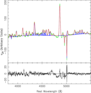
Figure 6.— Fitting of eigenspectrum 3. The top panel shows the mean eigenspectrum 3 (green) and the model (red), which consists of three components (blue), including a Legendre polynomial “continuum,” a set of Gaussians to represent Fe ii and Balmer lines, and a set of Gaussians with negative intensity to represent the [O iii] lines that arise from cross talk. The bottom panel shows the residuals.

As shown in Figure 6, the mean eigenspectrum 3 can be fitted well with the following three components. (1) A Legendre polynomial to model the “continuum.” (2) A set of single Gaussians with the same velocity shift and width, the intensities of which are free to vary. Each Gaussian is an emission line, including Balmer lines from H$\beta$ to H$\eta$, and Fe ii lines. We assemble the line list for Fe ii from Véron-Cetty et al. (2004) and Sigut & Pradhan (2003). (3) Another set of lines, each of which is modeled by a single Gaussian with negative intensity and fixed width and shift, to represent the cross-talk features at the location of [O iii] $\lambda\lambda$4959, 5007 and [Ne iii] $\lambda$3869.

Excluding the cross talk component (the third component above), the emission lines in eigenspectrum 3 can be fitted well using a single Gaussian with identical width and shift. This finding strongly supports our proposition, based on the phenomenological analysis in §4.1, that eigenspectrum 3 represents an independent, physically distinct emission component characterized by intermediate velocities.

Our fits yield a list of emission-line intensity ratios, one that, as in Véron-Cetty et al. (2004) and Dong et al. (2011), can be easily used as a template to model real quasar spectra. If only the Fe ii lines in the list are used, it works as an optical Fe ii template. This application will be discussed in the second paper of this series. A more interesting application is to combine both the Fe ii and the Balmer lines into a single template for the intermediate-line region. Such an approach would assume that the H$\beta$ to Fe ii intensity ratio is roughly constant in the intermediate-line region for different sources. This is possible if the clouds that emit intermediate-velocity lines have large column densities, as suggested by Ferland et al. (2009), who predict that the outward emission reaches an asymptotic value of Fe ii/H$\beta$ $\approx$ 3 (see their Figure 3). If this assumption is tenable, the Fe ii emission can be used to constrain the intermediate-width component of H$\beta$, thereby enabling a more physically motivated strategy for decomposing the H$\beta$ profile. This is relevant for black hole mass estimation and will be explored in the third paper of this series.

5. Simulations

Simulations with artificial spectra are used in the literature to test the validity and limitations of using the SPCA method for physical interpretation (e.g., Mittaz et al., 1990; Brotherton et al., 1994; Shang et al., 2003). While SPCA is successful in recognizing independent sets of correlated emission features, it is widely acknowledged that the interpretation is severely complicated by cross talk (e.g., the negative narrow features in our eigenspectrum 3; Figure 2(d)). More seriously, different eigenspectra, such as SPC1 and SPC3 in Shang et al. (2003) or the intermediate-line region component in Brotherton et al. (1994), cannot be uniquely attributed to distinct physical components. While these eigenspectra can be ascribed to independently varying components, as we do in our study, this interpretation is not unique. They can also be produced by a single emission-line component whose width becomes broader with lower peak flux (see Figure 13 of Shang et al. 2003).

In §3 above, we introduce the fractional-contribution spectra matrix $\mathbf{P}$ (calculated by Equation [C7] in Appendix C), which, as shown in §4.1, facilitates recognition of emission features in the eigenspectra. In this section we add $\mathbf{P}$ to simulations to investigate if it can be helpful in (1) distinguishing cross talk and (2) constraining the single emission-line region model.

In order to mimic real SDSS data, we generate artificial spectra using the same method described in §3.3 of Hu et al. (2008b). We add Gaussian random noise using a realistic noise pattern that is generated by scaling a real error array taken from SDSS observations to match the desired S/N of the simulation, and we adopt a realistic mask array. To match our SPCA sample, the redshift and S/N of the spectra are randomly set to be uniformly distributed as $z\sim\rm{U}(0.1,0.67)$ and $\rm{S/N}\sim\rm{U}(10,20)$. Fe ii emission is modeled by Gaussian broadening, scaling, and shifting the template constructed by Boroson & Green (1992). All the other emission-line components have a Gaussian profile. The distributions of EWs are chosen to be consistent with those in the real SDSS sample. In each case below, 1000 spectra are generated for SPCA. Table 3 summarizes the models and parameters of each simulation below.

Table 3Models and parameters of the simulations

	Power law	Fe ii	[O iii]	${\rm H}\beta_{\rm BC}^{1}$		${\rm H}\beta_{\rm BC}^{2}$
Case	$\alpha$	EW	EW	EW	FWHM	EW	Results
1(a)	0	$\rm{U}(25,75)$	$\rm{U}(0,20)$	$\cdots$	$\cdots$	$\cdots$	Fig. 7(a)
1(b)	0	$\rm{U}(25,75)$	20-0.2EW(Fe ii)	$\cdots$	$\cdots$	$\cdots$	Fig. 7(b)
1(c)	0	$\rm{U}(25,75)$	($\rm{U}(0,20)$ + 20-0.2EW(Fe ii))/2	$\cdots$	$\cdots$	$\cdots$	Fig. 7(c)
2	$\rm{U}(-2.5,-0.5)$	$\rm{U}(25,75)$	$\cdots$	$\rm{U}(20,100)$	$10^{3.35}$EW(H$\beta$)/EW(Fe ii)	$\cdots$	Fig. 10
3	$\rm{U}(-2.5,-0.5)$	$\rm{U}(25,75)$	$\rm{U}(0,20)$	0.5EW(Fe ii)	FWHM(Fe ii)	$-40\alpha$	Fig. 11

Note. —  $\cdots$  means not included in the specific model.

5.1. Cross Talk

The aim of the first series of simulations is to study the behavior of the fractional-contribution spectrum, to see whether it can help distinguish between cross talk from a genuine inverse correlation when absorption-like features such as those in eigenspectrum 3 are detected. We begin with the simplest case, a spectrum consisting of a continuum set to unity and only two emission-line components, Fe ii and [O iii]. The FWHMs of the lines are fixed to 1500 $\rm km~{}s^{-1}$ and 400 $\rm km~{}s^{-1}$, respectively, and no shifts are considered. Only the EWs vary: EW(Fe ii) $\sim\rm{U}(25,75)$ Å, and according to how EW([O iii]) is generated, three different simulations are performed (Table 3, case 1).

• The EW of [O iii] is independent from that of Fe ii:

  $${\rm EW}([\textsc{O iii}])={\rm EW}_{1}\sim{\rm U}(0,20)~{}\mathring{\rm A}.$$ (1)

• The EW of [O iii] is dependent on that of Fe ii:

  $${\rm EW}([\textsc{O iii}])={\rm EW}_{2}=20-0.2{\rm EW}({\rm Fe}~{}\textsc{ii}).$$ (2)

• The EW of [O iii] is semi-dependent on that of Fe ii:

  $${\rm EW}([\textsc{O iii}])=({\rm EW}_{1}+{\rm EW}_{2})/2.$$ (3)

Figure 7.— Results of the simulations for cross talk. Panels (a), (b), and (c) show the resultant eigenspectra when the EW of [O iii] depends differently on the EW of Fe ii, as indicated by the labels above the panels. Note the different fractional contribution ($p$) at the wavelength of [O iii].

Figure 7 shows the results of the three simulations. The three eigenspectra all show positive Fe ii emission and negative [O iii] lines. Although the strengths of the negative [O iii] features relative to Fe ii are different in the three cases, nothing essential can be distinguished. But the three fractional-contribution spectra show remarkable differences at the positions of [O iii] lines: zero in case (a), close to 100% in case (b), and $\sim$ 40% in case (c). Thus the fractional-contribution spectrum, which describes the contribution of eigenspectra to emission features, effectively distinguishes between cross talk and real correlation.

Figure 8.— EW of Fe ii versus EW of [O iii] for our sample used for SPCA analysis. The lack of a strong correlation suggests that the negative narrow [O iii] feature in our eigenspectrum 3 is not caused by BG92’s EV1.

Eigenspectrum 3 of our sample (Figure 2(d)) resembles case (a) here. The fractional-contribution spectrum goes almost to zero for [O iii], meaning that the negative [O iii] features arise only from cross talk and do not reflect any intrinsic inverse correlation between Fe ii and [O iii]. But where is BG92’s EV1 in our eigenspectra? We believe that this signature is absent from our sample because of selection effects. By design, our sample is biased toward objects with strong Fe ii (§2.2), and hence we do not expect to find a strong inverse correlation between the strengths of Fe ii and [O iii]. Figure 8 confirms this expectation; EW(Fe ii) and EW([O iii]) are only correlated at the level of $r_{\rm P}=-0.175$. This correlation is much weaker than those between Balmer lines, narrow emission lines, or Fe ii lines, thus will not appear in the first three eigenspectra.

5.2. The Single H$\beta$ Component Model

Figure 9.— Correlation diagram for FWHM(${\rm H}\beta_{\rm BC}$) versus $R_{\rm Fe}$. The solid line is the fit to the data as given in Equation (4).

Before describing the second simulation, which is aimed at ruling out the single Balmer line component model, we plot the correlation diagram for FWHM(${\rm H}\beta_{\rm BC}$) versus $R_{\rm Fe}$, defined as the ratio between the EW of Fe ii and the EW of ${\rm H}\beta_{\rm BC}$ (Figure 9). There is a rather strong inverse correlation ($r_{\rm P}=-0.507$), which, from an OLS bisector fit, can be described by

$${\rm FWHM}({\rm H}\beta_{\rm BC})=10^{(3.35\pm 0.01)}~{}{R_{\rm Fe}}^{(-1.05\pm 0.02)}.$$ (4)

This correlation has been found before (e.g., Boroson & Green, 1992; Sulentic et al., 2000a, and references therein), but its physical interpretation is still far from conclusive. There are two possible phenomenological interpretations. The straightforward explanation is that there is only a single H$\beta$ component whose width varies systematically with the relative strength of Fe ii and H$\beta$. Alternatively, H$\beta$ has two kinematic components, and the intensity of the narrower one scales with that of Fe ii by some fixed ratio, while the broader one varies independently. In this scenario, larger $R_{\rm Fe}$ means that H$\beta$ has a stronger narrow component relative to its broader component, making the whole H$\beta$ profile narrower. Previous SPCA studies have claimed that eigenspectra such as our eigenspectra 1 and 3 can be produced by either of the models above. There was no definitive way to discriminate between the two.

Here we aim to use our SPCA results to distinguish between these two phenomenological models, with the help of the fractional-contribution spectra $\mathbf{P}$. We generate artificial spectra that consist of three emission components (Table 3, case 2):

• Fe ii emission whose EW $\sim\rm{U}(25,75)$ Å;

• an H$\beta$ component whose EW $\sim\rm{U}(20,100)$ Å and FWHM $=10^{3.35}{R_{\rm Fe}}^{-1}$, according to Equation (4);

• a power-law continuum whose $f_{5100}$ flux density is fixed to unity but slope varies in the range $\alpha\sim\rm{U}(-2.5,-0.5)$.

A varying power law is added here to mimic real spectra more realistically than in the first series of simulations in the last subsection, and it helps us achieve our goal, as shown below.

Figure 10.— Results of the SPCA simulation for a single-component H$\beta$ line whose width correlates with $R_{\rm Fe}$. The labels are the same as those in Figure 2. While the mean spectrum resembles that of Figure 2, the first three eigenspectra and their corresponding fractional-contribution spectra differ. Note that the simulation here does not take into account the [O iii] lines. See text for details.

Figure 10 shows the mean spectra and the first three eigenspectra given by SPCA. As in Figure 2, the lower panels show the proportion of intrinsic variation and the fractional-contribution spectra. Considering that we do not account for the [O iii] lines in the simulation, the mean spectra and proportion of intrinsic variation here resembles that in Figure 2. There are three main differences between these SPCA results based on simulated spectra compared to those derived from real spectra. First, the eigenspectrum 1 here shows only a clean power law; some emission lines that correlate with the continuum are missing. Second, eigenspectrum 2 highlights the wings of the Balmer lines. And third, eigenspectrum 3, which contains Fe ii emission, shows a “W” shape at H$\beta$, and, as shown by the fractional-contribution spectrum, contributes a lot to the variation of H$\beta$ wings.

In conclusion, a single Balmer emission-line component whose width simply correlates with its strength with respective to Fe ii generates simulated eigenspectra that do not match well with our observed results in any of the first three eigenspectra and fractional-contribution spectra.

5.3. Reproduction of Our SPCA Results

The simulation above suggests that neither a single Balmer emission-line component nor two independently varying components can produce our SPCA results shown in Figure 2. A Balmer line component that correlates with the power-law continuum plus another that correlates with Fe ii emission are needed. We demonstrate this using the simulation below.

As listed on the last line of Table 3, the artificial spectra are composed of the following five components:

• a power-law continuum with specific flux density $f_{5100}$ fixed to unity but slope $\alpha\sim\rm{U}(-2.5,-0.5)$;

• Fe ii emission with EW $\sim\rm{U}(25,75)$ Å and a fixed FWHM = 1500 $\rm km~{}s^{-1}$;

• [O iii] emission with EW $\sim\rm{U}(0,20)$ Å  and a fixed FWHM = 400 $\rm km~{}s^{-1}$;

• a Balmer component with EW set to $0.5$EW(Fe ii) and FWHM fixed to that of Fe ii;

• a broader Balmer component with EW $=-40\alpha$ and a fixed FWHM $=4500$ $\rm km~{}s^{-1}$.

The fourth component depends on the second, and the fifth is determined by the first. Thus, there are only three free parameters: the slope of the power-law continuum, the strength of the Fe ii emission, and the strength of the narrow [O iii] lines.

Figure 11.— Results of the SPCA simulation aimed at reproducing the eigenspectra of the observed sample. The labels are the same as those in Figure 2. The first three eigenspectra are sufficient to account for the intrinsic variation. Ignoring the emission features that are not included in the simulation (e.g., [O ii] emission, higher order Balmer lines, Balmer continuum, etc.), the mean spectrum, the eigenspectra, and the fractional-contribution spectra closely resemble their observed counterparts in Figure 2.

Figure 11 shows the derived SPCA results. The first three eigenspectra, added up, account for 82.40% of the total variation, and are sufficient for describing the intrinsic variation (82.26% of the total). This is consistent with the number of free parameters included in the simulation. Comparing the results here with those in Figure 2, this simulation successfully reproduces the SPCA results for the real SDSS spectra, including almost all of the main features in the mean spectrum, the first three eigenspectra, and the fractional-contribution spectra.

These simulations strongly confirm the validity of the fractional-contribution spectrum and verify our interpretation of the eigenspectra in §4. They support the notion that two Balmer emission-line components are needed to reproduce our SPCA results: (1) a broader one that correlates with the power-law continuum and produces no Fe ii emission and (2) a narrower one that has the profile of, and correlates with, Fe ii.

6. Results for Large Fe ii Velocity Shifts

Aside from the primary sample of quasars with small Fe ii velocity shift, four other samples with larger Fe ii velocity shifts are also established in §2.2. This section presents the results of SPCA for these four samples, which can be understood easily in light of the analysis and simulations for the primary sample above.

Figure 12.— The first three eigenspectra and corresponding fractional-contribution spectra for the four bins of large Fe ii velocity shift. The range of Fe ii velocity shift in each bin is labeled on the left of each row. The percentage in each panel indicates the contribution of the eigenspectrum over the entire wavelength range. The number of objects in each of the four bins is given in the panels of the middle column.

Figure 12 shows the first three eigenspectra and corresponding fractional-contribution spectra for the four new velocity bins. Sample B (with Fe ii velocity shifts between 250 and 750 $\rm km~{}s^{-1}$) has roughly equal size (794 objects) as the primary sample. The results of SPCA for this sample resemble those for the primary sample, for example, in terms of the contributions of the eigenspectra over the entire wavelength range (59.9%, 15.3%, and 4.0%), the shapes and intensities of the first three eigenspectra, and fractional-contribution spectra. Thus, the first three eigenspectra represent the same emission components described in §4.1.

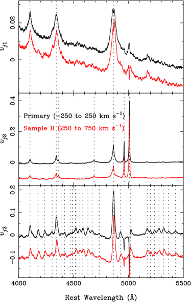
Figure 13.— Comparison between the first three eigenspectra of the primary sample (in black) and sample B (in red). The eigenspectra of sample B are shifted vertically for clarity. The dotted lines mark the rest wavelengths of major emission lines encoded in the eigenspectra (top panel: Balmer lines; middle panel: Balmer lines, He ii $\lambda$4686, [O iii] $\lambda$ 4363, and [O iii] $\lambda\lambda$4959, 5007; bottom panel: Balmer lines, and Fe ii lines). Note the redshift of eigenspectrum 3 of sample B.

In Figure 13, we compare the first three eigenspectra of sample B (in red, vertically shifted) to those of the primary sample (in black). The rest wavelengths of major emission lines are marked by dotted lines. Top and middle panels show that eigenspectra 1 and 2 of the two samples are almost the same. None of the major emission lines (very broad Balmer lines in eigenspectrum 1; narrow Balmer lines, He ii, and [O iii] lines in eigenspectrum 2) have a significant velocity shift between the two samples. The only notable difference is seen in eigenspectrum 3. The Fe ii lines and the intermediate-width Balmer lines of sample B are redshifted by $\sim 400$ $\rm km~{}s^{-1}$ with respect to the primary sample. This is expected because the two samples are divided by Fe ii velocity shift and the third eigenspectrum represents the intermediate-width emission lines, which mainly include Fe ii. It provides additional evidence that the measurement of Fe ii velocity shift in Hu et al. (2008b) is reliable in these two samples. Note that the negative features of [O iii] arise from cross talk, not redshift.

The three bins with larger Fe ii velocity shift contain relatively fewer objects: 338, 203, and 110 in samples C, D, and E, respectively. The eigenspectra and fractional-contribution spectra of these three samples are very similar. Their first two eigenspectra and fractional-contribution spectra resemble those of the primary sample (judging from the fractional-contribution spectra, note that the [O iii] lines in eigenspectra 1 arise just from cross talk), while fractional-contribution spectra 3 are different. Eigenspectra 3 of these three samples contribute little in terms of Fe ii emission. Their contributions over the entire wavelength range are also minimal. Thus, eigenspectra 3 of samples C, D, and E do not record the intermediate-width component. This is reasonable because EW(Fe ii) in the three samples is small and H$\beta$ is rather broad (Hu et al., 2008b) and tends to have single-Gaussian profiles (Figure 1(a) of Hu et al. 2008a). The intermediate-width component is expected to be weak, contributes little to the total variation, and can be easily smeared by nonlinear factors. This interpretation is supported by the fact that the first two eigenspectra have already contributed a larger proportion of variation ($\gtrsim$ 80%) than the first three eigenspectra of the primary sample (78.4%).

In conclusion, the results of SPCA for sample B resemble those for the primary sample, except that eigenspectrum 3 is redshifted. For the other three samples, only the first two eigenspectra are important; they record the power-law continuum $+$ very broad emission lines and narrow emission lines, respectively.

7. Discussion

Our SPCA analysis is based on the quasar sample of Hu et al. (2008b), which is intentionally biased toward objects with strong Fe ii emission [EW(Fe ii) $>25$ Å] to facilitate measurement of Fe ii velocity shifts. Given this situation, it is important to ask whether the principal result of this paper, namely that the Balmer lines contain two physically distinct components, is unique to our sample or applies to the quasar population in general. The key test of this scenario is to perform a detailed decomposition of the broad H$\beta$ profile, to isolate the two kinematic components. We defer this analysis to the second paper of this series, where we will explore the feasibility of using the eigenspectrum 3 derived here as a template to model the intermediate-velocity component of the spectrum.

In the meantime, we will use two samples selected differently from that used in our SPCA analysis to argue that our main conclusions are robust against sample selection effects.

7.1. Intermediate-line Region

Our analysis posits that the traditional BLR consists of two components, one with intermediate velocities in which H$\beta$ and Fe ii coexist with roughly constant relative intensity, and another characterized by larger velocities that emits H$\beta$ but no Fe ii. The relative contribution of these two components varies from source to source. A simple consequence of this picture is that the EW of the total broad H$\beta$ line should be larger than a factor times that of Fe ii. We construct a sample from the SDSS DR5 quasar catalog using the same criteria of Hu et al. (2008b), as described in §2.2, except that we impose no restriction based on EW(Fe ii). Thus, this sample is not biased toward objects with strong Fe ii emission.

Figure 14.— EW of ${\rm H}\beta_{\rm BC}$ versus that of Fe ii. This sample is selected from the SDSS DR5 quasar catalog by the same criteria of those in Hu et al. (2008b), except that no cut is made for EW(Fe ii). The solid line denotes EW(${\rm H}\beta_{\rm BC}$) $=0.5$ EW(Fe ii). Fewer than 1% of the sources lie below this line.

Figure 14 shows the relation between ${\rm H}\beta_{\rm BC}$ and Fe ii EWs for this sample. As in Figure 4, we measure ${\rm H}\beta_{\rm BC}$ by Gauss-Hermite fitting, which accounts for the full broad H$\beta$ profile. The distribution of points in the plot shows a clear lower boundary, which is approximately delineated by EW(${\rm H}\beta_{\rm BC}$) $=0.5$ EW(Fe ii). Only 47 sources out of 4757 (fewer than 1%) lie below the line. The existence of this bottom boundary is consistent with our two-component scenario if the strength of the intermediate-width H$\beta$ component is roughly a fixed fraction of Fe ii. Furthermore, our simulations confirm that such an assumption reproduces well the eigenspectra of the real data.

7.2. Correlation Between Strength of Very Broad H$\beta$ and $\alpha$

A correlation between the EW of broad H$\beta$ and the optical continuum slope $\alpha$ has seldom been reported in the literature, and the few papers that have mentioned it have given inconsistent results. Srianand & Kembhavi (1997), for example, found no correlation between optical spectral index and the EW of H$\beta$, but Francis et al. (2001) reported that the EW of H$\beta$ increases as the continuum becomes bluer. Our finding that the EW of very broad H$\beta$ correlates with $\alpha$ does not necessarily contradict with previous studies because no H$\beta$ decomposition was done before, not to mention that the samples are different. Richards et al. (2003) found that H$\beta$ line width decreases in quasars with redder continuum; this trend is qualitatively consistent with our scenario insofar as bluer objects exhibit a stronger very broad H$\beta$ component and hence a broader overall line profile.

The sources with EW(Fe ii) $<25$ Å in Figure 14 comprise quasars with weak Fe ii emission; they formally lie outside of the selection criterion of Hu et al. (2008b). Within the framework of this study, this subsample of weak-Fe ii sources should have a weak intermediate-width H$\beta$ component, and their broad H$\beta$ emission should be dominated by the very broad component. This subsample is convenient for testing the inverse correlation between the strength of the very broad H$\beta$ component and the slope of the power-law continuum, without having to perform accurate profile decomposition.

Figure 15.— Correlation diagram for the EW of entire broad H$\beta$ line versus the slope of the power-law continuum ($\alpha$, defined as $f_{\lambda}\propto\lambda^{\alpha}$) for sources with EW(Fe ii) $<25$ Å in Figure 14. The inverse correlation is strong. The solid line shows the OLS bisector fit.

Figure 15 confirms our expectations. We find a strong inverse correlation between EW(${\rm H}\beta_{\rm BC}$) and $\alpha$, with Pearson’s correlation coefficient $r_{\rm P}=-0.463$. An OLS bisector fit yields

$${\rm EW}({\rm H}\beta_{\rm BC})=(17.5\pm 2.7)-(41.6\pm 1.3)\alpha.$$ (5)

This empirical result motivated one of the input criteria (the fifth) for the simulation described in §5.3.

A bluer continuum has more ionizing photons relative to the non-ionizing continuum at 5100 Å, to which the EWs in the present paper all refer. Thus, an inverse correlation between the EW of an emission line and $\alpha$ arises naturally if the line-emitting clouds are optically thick to, and photoionized by, the same continuum that we see, and the clouds emits isotropically. On the other hand, the lack of any correlation between the intermediate-width component and the continuum slope reflects the complexity of the dynamics (Hu et al., 2008b) and physics (e.g., Baldwin et al., 2004; Ferland et al., 2009, and reference therein) of the Fe ii-producing gas. These two different dependences on spectral slope, in conjunction with the distinct locations and dynamics implied by their different velocity widths and shifts, indicate that the two components may respond very differently to continuum variations. This has been suggested by the reverberation analysis of Fe ii emission in Ark 120 (Kuehn et al., 2008), and also by recent studies that investigate the time delay between different velocity components of H$\beta$ and the continuum (Zhang, 2011; Wang & Li, 2011). Velocity-resolved time-delay measurements in some sources also show that H$\beta$ originates from structures more complicated than a single virialized region (e.g., Bentz et al., 2010; Denney et al., 2010, and reference therein).

The width of the broad H$\beta$ emission line has been widely used to estimate virial velocities to derive BH masses in AGNs. Our two-component model for the H$\beta$-emitting region raises an important question: which component better traces the virialized portion of the BLR? Our SPCA results suggest that the very broad component is more appropriate for BH mass estimation. We will investigate this problem in the third paper of this series.

8. Summary

We select a sample of 816 quasars with small Fe ii velocity shift from SDSS and perform spectral principal component analysis (SPCA) on this sample in rest wavelength range 3500–5500 Å. Apart from adjusting some details in the SPCA algorithm, we introduce, for the first time, a parameter called the fractional-contribution spectrum that measures the proportion of the variation accounted for by an eigenspectrum in a wavelength bin. We demonstrate the utility of this new parameter in helping to interpret the eigenspectra. We explore the correlations between the weights of the eigenspectra and various physical quantities to confirm the physical meaning of the eigenspectra. We perform a bootstrap analysis, spectral fitting of the eigenspectra, and Monte Carlo simulations to test the uncertainty of the eigenspectra, the validity of the fractional-contribution spectrum we introduced, and the two-component model of the H$\beta$-emitting region we propose.

Our principal findings from SPCA are as follows.

1. The first three eigenspectra have clear physical meanings. Eigenspectrum 1 represents the power-law continuum, very broad Balmer emission lines, and the correlation between them. Eigenspectrum 2 represents narrow emission lines. Eigenspectra 3 consists of Fe ii lines and Balmer lines with kinematically similar intermediate velocities.

2. The fractional-contribution spectrum is a powerful tool for diagnosing the emission features represented in each eigenspectrum, as well as for recognizing spurious features that arise from cross talk.

3. The broad H$\beta$ line consists of two physically distinct components: a very broad component whose strength correlates with the slope of the optical power-law continuum, and an intermediate-width component that has the profile of, and correlates with, Fe ii.

While our current sample is biased toward objects with strong Fe ii emission, we argue that our overall findings are immune from strong sample selection bias and are generally applicable to the general quasar population. This means that the strength of the intermediate-width H$\beta$ component varies from source to source and could vanish. In extreme cases H$\beta$ only has a single Gaussian component. We will rigorously test this conclusion in a forthcoming work, where we will perform detailed spectral decomposition using the new template spectrum for Fe ii emission and intermediate-velocity Balmer lines derived from eigenspectrum 3.

The two-component nature of the broad H$\beta$ line raises important concerns about the robustness of current virial BH mass estimates that make use of the H$\beta$ line width. This issue will be explored in another forthcoming publication.

Appendix A Evidence for Redshifted Fe ii Emission in Quasars from Composite Spectra

Sulentic et al. (2012) called into question the measurement of Fe ii velocity shifts ($v_{\rm Fe}$) in Hu et al. (2008b). They raised two criticisms. First, they argue that the majority of the sources in Hu et al. (2008b) do not have enough S/N to yield a reliable measurement of $v_{\rm Fe}$. Second, they note that Hu et al. (2008b) did not include He ii emission in their fits. Sulentic et al. (2012) generated composite spectra, which have high S/N, of several subsamples defined by their 4D Eigenvector 1 formalism, and then measured $v_{\rm Fe}$ from fits of the composite spectra that include the He ii line. They concluded that the Fe ii emission in their composite spectra do not have significant velocity shifts. In this Appendix, we adopt similar fitting methods, take He ii into consideration, measure $v_{\rm Fe}$ for the five composite spectra generated in Hu et al. (2008b), and test the statistical significance of our measurement of $v_{\rm Fe}$. We confirm that our redshift measurements of Fe ii are robust.

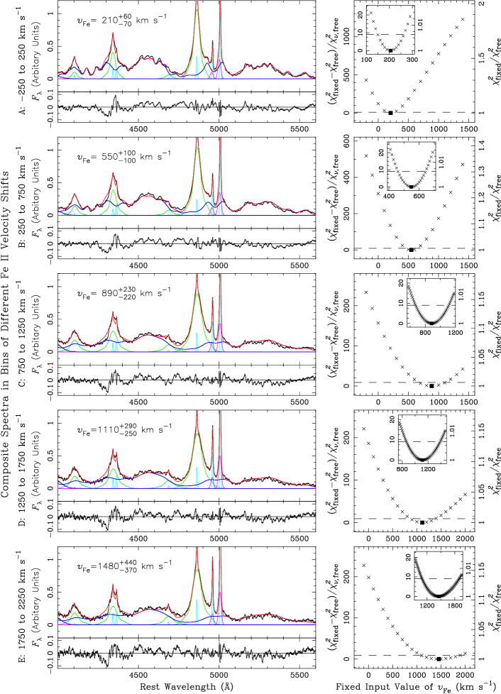
Figure 16.— (Left) Fits of composite spectra made by assuming $v_{\rm Fe}$ is free. The composite spectra were generated in Hu et al. (2008b) by stacking the spectra of quasars in bins of different measured $v_{\rm Fe}$. The range in each bin is labeled on the left of each row. For each bin, the top panel shows the continuum-subtracted composite spectrum (black) and best-fit model (red), including Fe ii emission (blue), broad emission lines (green), narrow emission lines (cyan), and wings of [O iii] lines (magenta). The bottom panel shows the residuals. (Right) $\chi^{2}$ curve (crosses) for the fits with fixed $v_{\rm Fe}$; the insert zooms in around the minimum. The horizontal dashed line marks where the difference in $\chi^{2}$ has 3$\sigma$ significance. The value of the best-fit $v_{\rm Fe}$ (solid square) and its 3$\sigma$ confidence interval (where the $\chi^{2}$ curve intersects the dashed line) are labeled in the panel showing the fit. Note that the range of the abscissa of the $\chi^{2}$ curves for the last two composite spectra are different with those for the first three.

The details of the five composite spectra are described in §4.6 of Hu et al. (2008b). Briefly, the composite spectra are geometric means (Vanden Berk et al., 2001) of the spectra of quasars in five bins of different $v_{\rm Fe}$ measured in Hu et al. (2008b): $-$250 to 250 $\rm km~{}s^{-1}$ (A, 1350 objects), 250 to 750 $\rm km~{}s^{-1}$ (B, 1362 objects), 750 to 1250 $\rm km~{}s^{-1}$ (C, 590 objects), 1250 to 1750 $\rm km~{}s^{-1}$ (D, 332 objects), and 1750 to 2250 $\rm km~{}s^{-1}$ (E, 180 objects). Our fitting method here resembles that in Hu et al. (2008b) but is improved in two aspects: (1) the He ii line is included and (2) the power-law continuum, Fe ii emission, and other lines are fitted simultaneously. The left column of Figure 16 shows our results. For each velocity shift bin, the top panel shows the continuum-subtracted composite spectrum (black) and best-fit model (red). Besides the power-law continuum, the model contains the following components: (1) Fe ii emission (blue) modeled by broadening, scaling, and shifting the I Zw 1 Fe template constructed by Boroson & Green (1992), (2) broad emission lines (green) modeled by a set of Gaussian-Hermite functions representing H$\beta$ $\lambda$4861, H$\gamma$ $\lambda$4340, H$\delta$ $\lambda$4102, and He ii $\lambda$4686, (3) narrow emission lines (cyan) modeled by a set of single Gaussians representing H$\beta$, H$\gamma$, H$\delta$, [O iii] $\lambda\lambda$4959, 5007, [O iii] $\lambda$4363, and He ii $\lambda$4686, and (4) wings of the [O iii] lines (magenta) modeled by a set of single Gaussians. The lines in each set have the same shape and shift, but different intensities. The bottom panel shows the residuals. The fitting is performed in the wavelength window 4000–5600 Å.

The significance of the measured $v_{\rm Fe}$ can be tested by using a $\chi^{2}$ statistic to determine whether the model with varying $v_{\rm Fe}$ fits the data better than the model with $v_{\rm Fe}$ fixed to a specific value (with other parameters left free). We use the $F$-test described in §11.4 of Bevington & Robinson (2003). In the fitting described above, if $v_{\rm Fe}$ is free to vary the best fit has chi-square $\chi^{2}_{\rm free}$ with 1435 degrees of freedom, and the reduced chi-square $\chi^{2}_{\nu,{\rm free}}=\chi^{2}_{\rm free}/1435$. If we fix $v_{\rm Fe}$ to a constant but allow all other parameters to vary and fit the composite spectra again, the new best fit has chi-square $\chi^{2}_{\rm fixed}$ with 1435$+$1 degrees of freedom. From Equation 11.50 of Bevington & Robinson (2003), the quantity

$$F_{\chi}=(\chi^{2}_{\rm fixed}-\chi^{2}_{\rm free})/\chi^{2}_{\nu,{\rm free}}$$ (A1)

follows a $F_{1,\nu_{2}}$ distribution, where $\nu_{2}=1435$ in this case. Thus, the probability that the model with varying $v_{\rm Fe}$ does not improve the fit compared to the model with $v_{\rm Fe}$ fixed to a specific value equals the probability of exceeding $F_{\chi}$ in an $F_{1,\nu_{2}}$ distribution, namely $P_{F}(F_{\chi};1,1435)$. From Figure C.5 of Bevington & Robinson (2003), the value of $F_{\chi}$ for $P_{F}(F_{\chi};1,1435)=1-99.73\%$ is approximately 9 (the $\nu_{2}=\infty$ curve); the precise number is 9.03. Thus, the best-fit value of $v_{\rm Fe}$ is significant at more than 3$\sigma$ confidence level if

$$(\chi^{2}_{\rm fixed}-\chi^{2}_{\rm free})/\chi^{2}_{\nu,{\rm free}}>9.03,$$ (A2)

or, equivalently,

$$\chi^{2}_{\rm fixed}/\chi^{2}_{\rm free}=F_{\chi}/dof+1>1.0063,$$ (A3)

where $dof$ is the number of degrees of freedom when $v_{\rm Fe}$ is free to vary (1435, in this case).

We fix $v_{\rm Fe}$ from $-$200 to 2000 $\rm km~{}s^{-1}$, obtain the best-fit chi-square $\chi^{2}_{\rm fixed}$ for each fixed input value of $v_{\rm Fe}$, and build up a $\chi^{2}$ curve for each composite spectrum, as shown in the right column of Figure 16 (crosses). For convenience, the chi-squares are plotted as $(\chi^{2}_{\rm fixed}-\chi^{2}_{\rm free})/\chi^{2}_{\nu,{\rm free}}$. The equivalent values of $\chi^{2}_{\rm fixed}/\chi^{2}_{\rm free}$ are also labeled on the right of the plot, for comparison with Figure 1 of Sulentic et al. (2012). The solid square marks the best-fit result when $v_{\rm Fe}$ is free to vary. The insert zooms in around the minimum of the $\chi^{2}$ curve. The 3$\sigma$ confidence interval of the $v_{\rm Fe}$ measurement can be determined by the two points when $(\chi^{2}_{\rm fixed}-\chi^{2}_{\rm free})/\chi^{2}_{\nu,{\rm free}}$ reaches 9.03 (marked by the horizontal dashed line). Fixing $v_{\rm Fe}$ to values outside of this velocity interval gives worse $\chi^{2}$ than setting $v_{\rm Fe}$ free, at 3$\sigma$ confidence level. The best-fit value of $v_{\rm Fe}$ when it is free to vary and its lower and upper 3$\sigma$ bounds are labeled in the panel on the left column.

For all five composite spectra the $\chi^{2}_{\rm fixed}$ when $v_{\rm Fe}$ is fixed to zero are significantly larger than $\chi^{2}_{\rm free}$ when $v_{\rm Fe}$ is allowed to vary. Thus, the Fe ii emission in the composite spectra do exhibit significant velocity shift. The resultant values of $v_{\rm Fe}$ (and its 3$\sigma$ confidence level) for the five composite spectra are $210_{-70}^{+60}$, $550_{-100}^{+100}$, $890_{-220}^{+230}$, $1110_{-250}^{+290}$, and $1480_{-370}^{+440}$ $\rm km~{}s^{-1}$. The measured $v_{\rm Fe}$ of the first three composite spectra are consistent with the velocity shift range of the bins, while those of the last two are slightly lower. This discrepancy is probably caused by the enhancement of the un-shifted spectral features (e.g., narrow emission lines and host galaxy component) during the stacking. Figure 12 of Hu et al. (2008b) shows that Ca ii absorption lines, produced by host galaxy starlight, are prominent in composites D and E. This shortcoming of the composite spectra has already been discussed in §4.6 of Hu et al. (2008b); it also explains why the velocity shifts of Fe ii cannot be seen by direct visual inspection.

He ii emission and host galaxy contamination may affect the $v_{\rm Fe}$ measurement in some individual cases. A thorough analysis of this problem, taking both factors into consideration, is beyond the scope of this paper. However, the fact that $v_{\rm Fe}$ is seen both in the composite spectra and it has a value similar to the velocity shift range used to stack the composite spectra suggest that the measurement of $v_{\rm Fe}$ in Hu et al. (2008b) is reliable for the majority of quasars. The values of $v_{\rm Fe}$ are thus suitable for the SPCA study in this paper. In fact, Hu et al. (2008b, their §3.3) had already tested the reliability of their $v_{\rm Fe}$ measurements for the S/N of SDSS spectra. Moreover, the influence of He ii emission is mitigated by the fact that Fe ii is fitted over a rather wide wavelength range.

We do not have a definitive explanation for the contradictory results obtained by Sulentic et al. (2012). Part of the problem may lie in the manner in which they constructed their composite spectra, which are defined by parameters of their 4D Eigenvector 1 formalism, namely H$\beta$ width and Fe ii/H$\beta$ intensity ratio. Figure 9 of Hu et al. (2008b) shows that these parameters are poorly correlated with $v_{\rm Fe}$. Thus, composite spectra generated in bins of these spectral properties are not equivalent to those constructed from bins in $v_{\rm Fe}$. We suspect that this may be the reason that Sulentic et al. (2012) failed to see the Fe ii velocity shifts reported by Hu et al. (2008b).

Appendix B Derivation of the Eigenspectra

This Appendix describe the detailed algorithm for deriving the eigenspectra. The algorithm basically follows that in Yip et al. (2004a).

After the three steps of spectra preprocessing described in §3, we prepare three $816\times 1962$ matrices: $\mathbf{F}$, $\boldsymbol{\Sigma}$, and $\mathbf{M}$, where $\mathbf{F}$ has element $f_{ij}$ as the flux of the $i$th mean-subtracted spectrum in the $j$th wavelength bin, and $\boldsymbol{\Sigma}$ and $\mathbf{M}$ specify the corresponding flux errors and masks given by the SDSS spectra. The goal of SPCA is to calculate the eigenvalues and eigenvectors of the correlation matrix $\mathbf{F}^{T}\cdot\mathbf{F}$:

$$(\mathbf{F}^{T}\cdot\mathbf{F})\cdot\mathbf{V}=\mathbf{V}\cdot(\boldsymbol{\Lambda}^{T}\cdot\boldsymbol{\Lambda}),$$ (B1)

where $\mathbf{F}^{T}$ denotes the transpose of matrix $\mathbf{F}$, $\mathbf{V}$ is an $n\times n$ orthogonal matrix whose columns ($\mathbf{v}_{k}$, $k=1,\ n$) are the eigenvectors of $\mathbf{F}^{T}\cdot\mathbf{F}$, $\boldsymbol{\Lambda}$ is an $n\times n$ diagonal matrix diag($\lambda_{1}\cdots\lambda_{n}$), and $\lambda_{k}^{2}$ are the eigenvalues of $\mathbf{F}^{T}\cdot\mathbf{F}$. This can be achieved using singular value decomposition (SVD):

$$\mathbf{F}=\mathbf{U}\cdot\boldsymbol{\Lambda}\cdot\mathbf{V}^{T},$$ (B2)

where $\mathbf{U}$ is an $m\times n$ column orthogonal matrix. Defining $\mathbf{W}=\mathbf{U}\cdot\boldsymbol{\Lambda}$, the mean-subtracted spectra can be reconstructed using the eigenspectra

$$\mathbf{F}=\mathbf{W}\cdot\mathbf{V}^{T},$$ (B3)

where $\mathbf{W}$ is an $m\times n$ matrix, $w_{ik}$ is the weight of the $k$th eigenspectrum for the $i$th mean-subtracted spectrum.

Next, we derive the eigenspectra iteratively, taking the errors $\boldsymbol{\Sigma}$ and masks $\mathbf{M}$ into account.

1. The bad pixels in the mean-subtracted spectra are initially corrected by mean interpolation, following Yip et al. (2004a). The flux of a bad pixel in any given spectrum is replaced by the mean of the fluxes of all the other spectra in the same wavelength bin, which is zero:

$$f_{ij}^{\rm c}=\sum_{i,\ {\rm good\ pixel}}f_{ij}~{}~{}~{}\bigg{/}\sum_{i,\ {\rm good\ pixel}}=0,$$ (B4)

for $i,j$ that $m_{ij}$ represents bad. The second equation holds because $\mathbf{F}$ is mean-subtracted. Actually, the choice of interpolation method for the initial bad pixel correction does not affect the resultant final eigenspectra. But the mean interpolation adopted here makes the convergence of eigenspectra faster (Yip et al., 2004a) and is quite simple (by just setting the flux to zero here).

2. The corrected flux matrix $\mathbf{F}^{\rm c}$ is then factorized in the form of Equation (B2) using the algorithm for SVD in chapter 2.6 of Press et al. (1992). Each column ($\mathbf{v}_{k}$) of the derived matrix $\mathbf{V}$ is an eigenspectrum; they are arranged in the order of decreasing eigenvalues $\lambda_{k}^{2}$.

3. The mean-subtracted spectra are reconstructed using the eigenspectra obtained, taking the errors and masks into account. For the $i$th spectrum, we find the set of $a_{ik}$ (the coefficient of the $k$th eigenspectra for the $i$th spectrum) by minimizing the quantity

$$\chi^{2}_{i}=\sum_{j,\ {\rm good\ pixel}}\left(\frac{f_{ij}-\sum_{k}a_{ik}v_{jk}}{\sigma_{ij}}\right)^{2}.$$ (B5)

This can be solved by Gauss-Jordan elimination (see §2 of Connolly & Szalay 1999 for details of the derivation). The reconstructed spectrum $f_{ij}^{\rm rec}=\sum_{k}a_{ik}v_{jk}$. In practice, only the first several tens eigenspectra are needed for reconstructing quasar spectra (Yip et al., 2004b; Boroson & Lauer, 2010). We find that the first 30 are sufficient for the case here (Figure 1 in §4.1).

4. The bad pixels in $\mathbf{F}$ are corrected again, using the reconstructed spectra obtained in the last step: $f_{ij}^{\rm c}=f_{ij}^{\rm rec}$. Then we cycle back to step 2 with the new $\mathbf{F}^{\rm c}$.

5. The loop in steps 2–4 iterates until the eigenspectra converge. Following Yip et al. (2004a), the commonality between the eigenspectra derived in the $n$th iteration ($\mathbf{V}^{n}$) and that in the $(n-1)$th iteration ($\mathbf{V}^{n-1}$) is defined as

$${\rm Tr}(\mathbf{S}^{n}\cdot\mathbf{S}^{n-1}\cdot\mathbf{S}^{n})/d,$$ (B6)

where Tr is the trace of a matrix, $d$ is the dimension of the two sets of eigenspectra for comparison, and $\mathbf{S}^{n}$ is the sum of the projection operators $\mathbf{V}^{n}$,

$$\mathbf{S}^{n}=\sum_{k=1}^{d}\mathbf{v}_{k}^{n}\cdot(\mathbf{v}_{k}^{n})^{T},$$ (B7)

where $\mathbf{v}_{k}^{n}$ is the $k$th eigenspectrum derived in the $n$th iteration. This quantity is unity if the two sets of eigenspectra are identical, and is zero if they are disjoint. It is not necessary to compare the entire set. We compare the first 30 eigenspectra for consistency with the reconstruction of the spectrum in step 3. After five iterations, ${\rm Tr}(\mathbf{S}^{5}\cdot\mathbf{S}^{4}\cdot\mathbf{S}^{5})/30=0.9997$ (see Figure 1 of Yip et al. 2004a for comparison). Thus, in this work, all eigenspectra are obtained with five iterations.

Appendix C The Fractional-contribution Spectrum

This paper introduces a new quantity, the fractional-contribution spectrum, which is useful for understanding eigenspectra. Here we present its definition in detail and compare it to other quantities widely used in the literature.

The total variation of the sample is defined as the sum of the squares of the differences between the normalized spectra and the mean spectrum:

$$var^{\rm tot}=\sum_{i,\ j}f_{ij}^{2}.$$ (C1)

It consists of two parts: one that accounts for the noise in the original spectra,

$$var^{\rm err}=\sum_{i,\ j}\sigma_{ij}^{2},$$ (C2)

and another that describes intrinsic variation, $var^{\rm int}=var^{\rm tot}-var^{\rm err}$. It is more straightforward to express them in percentages, such that $P^{\rm err}=var^{\rm err}/var^{\rm tot}$ and $P^{\rm int}=1-P^{\rm err}$.

The proportion of the variation accounted for by the $k$th eigenspectrum can be calculated as

$$P_{k}=\lambda_{k}^{2}/\sum_{l}\lambda_{l}^{2},$$ (C3)

where $\lambda_{k}^{2}$ is the eigenvalue for the $k$th eigenspectrum (Mittaz et al., 1990). This is the quantity used in previous SPCA studies, and it represents the contribution of an eigenspectrum to the total variation of the input spectra over the entire wavelength range. Thus, the first $n$th eigenspectra can account for $\sum_{k=1}^{n}P_{k}$ percentage of the total variation; it is called the cumulative proportion of variation and increases monotonically with $n$. When it reaches $P^{\rm int}$, it indicates that the first $n$ eigenspectra are sufficient for explaining the intrinsic variation in the sample, and the remaining higher order eigenspectra contribute only to noise and can be ignored for our purposes (see also §4.1).

The quantities defined above were widely used in previous SPCA studies, but they only refer to the average properties of the eigenspectra over the entire wavelength range. In this work, we develop these quantities to investigate the eigenspectra in each wavelength bin, as follows.

First, the total and noise variation in the $j$th wavelength bin can be simply defined as

$$var_{j}^{\rm tot}=\sum_{i}f_{ij}^{2},~{}~{}~{}var_{j}^{\rm err}=\sum_{i}\sigma_{ij}^{2};$$ (C4)

and

$$p^{\rm err}_{j}=var_{j}^{\rm err}/var_{j}^{\rm tot},~{}~{}~{}p^{\rm int}_{j}=1-p^{\rm err}_{j}.$$ (C5)

Second, after using the first $n$th eigenspectra for reconstruction, the residual variation in the $j$th wavelength bin is the sum of the square of the differences between the reconstructed spectra and mean-subtracted spectra in the specific wavelength bin:

$$var_{jn}^{\rm res}=\sum_{i}\left(f_{ij}-\sum_{k=1}^{n}a_{ik}v_{jk}\right)^{2}.$$ (C6)

The proportion of the variation accounted for by the $n$th eigenspectrum in the $j$th wavelength bin is

$$p_{jn}=\frac{var_{j(n-1)}^{\rm res}-var_{jn}^{\rm res}}{var_{j}^{\rm tot}}.$$ (C7)

As in the case applied to the entire wavelength range, these values are compared with $p_{j}^{\rm err}$ to determine the significance of each eigenspectrum.

Figure 17.— The sum of $p_{jk}$, weighted by $var_{j}^{\rm tot}$, versus $P_{k}$, expressed in percentage. $k$ increases from 1 to 30 from bottom left to top right. The two quantities, derived from our SPCA results, are almost equal. This implies that the previously used quantity $P_{k}$ can be considered as the $var_{j}^{\rm tot}$-weighted sum of $p_{jk}$. The new quantity $p_{jk}$ has the advantage that it contains more diagnostic power.

Thus, we obtain a matrix $\mathbf{P}$, which has the same shape as $\mathbf{V}$, whose element $p_{jk}$ represents the proportion of the variation accounted for by the $k$th eigenspectrum in the $j$th wavelength bin. Each column ($\mathbf{p}_{k}$) of $\mathbf{P}$ represents the contribution of the corresponding eigenspectrum and has the form of spectrum, we call it the fractional-contribution spectrum. Actually, as shown in Figure 17, the previously used $P_{k}$ can be considered as the sum of $p_{jk}$ weighted by $var_{j}^{\rm tot}$. The two quantities for the first 30 eigenspectra of our SPCA results are almost exactly equal ($k$ increases diagonally to the upper right).

References

- Adelman-McCarthy et al. (2007) Adelman-McCarthy, J. K., Agüeros, M. A., Allam, S. S., et al. 2007, ApJS, 172, 634
- Baldwin et al. (2004) Baldwin, J. A., Ferland, G. J., Korista, K. T., Hamann, F., & LaCluyzé, A. 2004, ApJ, 615, 610
- Bentz et al. (2010) Bentz, M. C., Walsh, J. L., Barth, A. J., et al. 2010, ApJ, 716, 993
- Bevington & Robinson (2003) Bevington, P. R., & Robinson, D. K. 2003, Data Reduction and Error Analysis for the Physical Sciences (3rd ed.; Boston, MA: McGraw-Hill)
- Boroson & Green (1992) Boroson, T. A., & Green, R. F. 1992, ApJS, 80, 109
- Boroson & Lauer (2010) Boroson, T. A., & Lauer, T. R. 2010, AJ, 140, 390
- Brotherton (1996) Brotherton, M. S. 1996, ApJS, 102, 1
- Brotherton et al. (1994) Brotherton, M. S., Wills, B. J., Francis, P. J., & Steidel, C. C. 1994, ApJ, 430, 495
- Cardelli et al. (1989) Cardelli, J. A., Clayton, G. C., & Mathis, J. S. 1989, ApJ, 345, 245
- Collin-Souffrin & Lasota (1988) Collin-Souffrin, S., & Lasota, J.-P. 1988, PASP, 100, 1041
- Connolly & Szalay (1999) Connolly, A. J., & Szalay, A. S. 1999, AJ, 117, 2052
- Connolly et al. (1995) Connolly, A. J., Szalay, A. S., Bershady, M. A., Kinney, A. L., & Calzetti, D. 1995, AJ, 110, 1071
- Denney et al. (2010) Denney, K. D., Peterson, B. M., Pogge, R. W., et al. 2010, ApJ, 721, 715
- Dong et al. (2011) Dong, X.-B., Wang, J.-G., Ho, L. C., et al. 2011, ApJ, 736, 86
- Ferland et al. (2009) Ferland, G. J., Hu, C., Wang, J.-M., et al. 2009, ApJ, 707, L82
- Francis et al. (2001) Francis, P. J., Drake, C. L., Whiting, M. T., Drinkwater, M. J., & Webster, R. L. 2001, PASA, 18, 221
- Francis et al. (1992) Francis, P. J., Hewett, P. C., Foltz, C. B., & Chaffee, F. H. 1992, ApJ, 398, 476
- Gaskell (1982) Gaskell, C. M. 1982, ApJ, 263, 79
- Hao et al. (2005) Hao, L., Strauss, M. A., Tremonti, C. A., et al. 2005, AJ, 129, 1783
- Hu et al. (2008a) Hu, C., Wang, J.-M., Ho, L. C., et al. 2008a, ApJ, 683, L115
- Hu et al. (2008b) Hu, C., Wang, J.-M., Ho, L. C., et al. 2008b, ApJ, 687, 78
- Isobe et al. (1990) Isobe, T., Feigelson, E. D., Akritas, M. G., & Babu, G. J. 1990, ApJ, 364, 104
- Kuehn et al. (2008) Kuehn, C. A., Baldwin, J. A., Peterson, B. M., & Korista, K. T. 2008, ApJ, 673, 69
- Ludwig et al. (2009) Ludwig, R. R., Wills, B., Greene, J. E., & Robinson, E. L. 2009, ApJ, 706, 995
- Mittaz et al. (1990) Mittaz, J. P. D., Penston, M. V., & Snijders, M. A. J. 1990, MNRAS, 242, 370
- Mullaney & Ward (2008) Mullaney, J. R., & Ward, M. J. 2008, MNRAS, 385, 53
- Netzer & Marziani (2010) Netzer, H., & Marziani, P. 2010, ApJ, 724, 318
- Netzer & Trakhtenbrot (2007) Netzer, H., & Trakhtenbrot, B. 2007, ApJ, 654, 754
- O’Donnell (1994) O’Donnell, J. E. 1994, ApJ, 422, 158
- Peterson & Wandel (1999) Peterson, B. M., & Wandel, A. 1999, ApJ, 521, L95
- Press et al. (1992) Press, W. H., Teukolsky, S. A., Vetterling, W. T., & Flannery, B. P. 1992, Numerical Recipes in FORTRAN (2nd ed.; Cambridge: Cambridge Univ. Press)
- R Core Team (2012) R Core Team (2012). R: A language and environment for statistical computing. R Foundation for Statistical Computing, Vienna, Austria. ISBN 3-900051-07-0, URL {http://www.R-project.org/}.
- Richards et al. (2003) Richards, G. T., Hall, P. B., Vanden Berk, D. E., et al. 2003, AJ, 126, 1131
- Richards et al. (2011) Richards, G. T., Kruczek, N. E., Gallagher, S. C., et al. 2011, AJ, 141, 167
- Salviander et al. (2007) Salviander, S., Shields, G. A., Gebhardt, K., & Bonning, E. W. 2007, ApJ, 662, 131
- Schneider et al. (2007) Schneider, D. P., Hall, P. B., Richards, G. T., et al. 2007, AJ, 134, 102
- Shang et al. (2003) Shang, Z., Wills, B. J., Robinson, E. L., et al. 2003, ApJ, 586, 52
- Sigut & Pradhan (2003) Sigut, T. A. A., & Pradhan, A. K. 2003, ApJS, 145, 15
- Spergel et al. (2007) Spergel, D. N., Bean, R., Doré, O., et al. 2007, ApJS, 170, 377
- Srianand & Kembhavi (1997) Srianand, R., & Kembhavi, A. 1997, ApJ, 478, 70
- Sulentic et al. (2000a) Sulentic, J. W., Marziani, P., & Dultzin-Hacyan, D. 2000a, ARA&A, 38, 521
- Sulentic et al. (2000b) Sulentic, J. W., Marziani, P., Zwitter, T., Dultzin-Hacyan, D., & Calvani, M. 2000, ApJ, 545, L15
- Sulentic et al. (2012) Sulentic, J. W., Marziani, P., Zamfir, S., & Meadows, Z. A. 2012, ApJ, 752, L7
- Vanden Berk et al. (2001) Vanden Berk, D. E., Richards, G. T., Bauer, A., et al. 2001, AJ, 122, 549
- Véron-Cetty et al. (2004) Véron-Cetty, M.-P., Joly, M., & Véron, P. 2004, A&A, 417, 515
- Vestergaard & Peterson (2005) Vestergaard, M., & Peterson, B. M. 2005, ApJ, 625, 688
- Wang & Li (2011) Wang, J., & Li, Y. 2011, ApJ, 742, L12
- Wang et al. (2011) Wang, L., Farrah, D., Connolly, B., et al. 2011, MNRAS, 411, 1809
- Yip et al. (2004a) Yip, C. W., Connolly, A. J., Szalay, A. S., et al. 2004a, AJ, 128, 585
- Yip et al. (2004b) Yip, C. W., Connolly, A. J., Vanden Berk, D. E., et al. 2004b, AJ, 128, 2603
- York et al. (2000) York, D. G., Adelman, J., Anderson Jr., J. E., et al. 2000, AJ, 120, 1579
- Zamfir et al. (2010) Zamfir, S., Sulentic, J. W., Marziani, P., & Dultzin, D. 2010, MNRAS, 403, 1759
- Zhang (2011) Zhang, X.-G. 2011, ApJ, 741, 104