Entropy-based Statistical Analysis of PolSAR Data

Abstract

Images obtained from coherent illumination processes are contaminated with speckle noise, with polarimetric synthetic aperture radar (PolSAR) imagery as a prominent example. With an adequacy widely attested in the literature, the scaled complex Wishart distribution is an acceptable model for PolSAR data. In this perspective, we derive analytic expressions for the Shannon, Rényi, and restricted Tsallis entropies under this model. Relationships between the derived measures and the parameters of the scaled Wishart law (i.e., the equivalent number of looks and the covariance matrix) are discussed. In addition, we obtain the asymptotic variances of the Shannon and Rényi entropies when replacing distribution parameters by maximum likelihood estimators. As a consequence, confidence intervals based on these two entropies are also derived and proposed as new ways of capturing contrast. New hypothesis tests are additionally proposed using these results, and their performance is assessed using simulated and real data. In general terms, the test based on the Shannon entropy outperforms those based on Rényi’s.

I Introduction

Polarimetric synthetic aperture radar (PolSAR) has been used to describe earth surface phenomena [1]. This technology uses coherent illumination which causes the interference pattern called ‘speckle’ [2], which is multiplicative by nature and, in the format here considered, is non-Gaussian. This fact precludes the use of conventional tools in PolSAR image analysis, requiring specialized techniques.

The scaled complex Wishart distribution has been successfully employed as a statistical model for homogeneous regions in PolSAR images. This law is at the core of segmentation [3], classification [4], and boundary detection [5] techniques.

The concepts of “information” and “entropy” were given formal mathematical definitions in the context of data communications by Shannon in 1948 [6]. Thenceforth, the proposition and application of information and entropy measures have become an active research field in several areas. Zografos and Nadarajah derived closed expressions for Shannon and Rényi entropies for several univariate [7], bivariate [8], and multivariate [9] distributions.

Exploring relationships associated with the log-likelihood function, Zong [10] applied the Rényi entropy to several univariate distributions. In fact, this entropy measure has been applied to image processing problems such as data mining, detection, segmentation, and classification [11, 12, 13]. Another prominent entropy measure is the restricted Tsallis entropy. This tool was introduced by Tsallis in [14, 15] and is related to the Rényi entropy. The restricted Tsallis entropy has found applications in statistical physics [16].

Among these information theoretical tools, the Shannon entropy has been applied to PolSAR imagery. Morio et al. [17] analyzed such entropy for the characterization of polarimetric targets under the complex, circular, and multidimensional Gaussian distribution.

Stochastic distances are also derived within the framework of information theory. A comprehensive examination of these measures is presented and applied to intensity SAR data in [18, 19], and to PolSAR models in [20].

In this paper, we derive analytic expressions for the Shannon, Rényi, and restricted Tsallis entropies under the scaled complex Wishart law. These measures are analyzed as particular cases of the ($h,\phi$)-entropy proposed by Salicrú et al. [21]. When parameters are replaced by maximum likelihood estimators, these entropies become random variables; expressions for the asymptotic variances of the Shannon and Rényi entropies are derived (the Tsallis entropy becomes analytically intractable and, thus, is no further considered).

Novel methodologies for testing hypotheses and constructing confidence intervals are proposed for quantifying contrast in PolSAR imagery using these results. Such measures can be used in PolSAR segmentation [3], classification [4], boundary detection [22, 23], and change detection [24]. Monte Carlo experiments are performed for assessing the performance of the discussed measures in synthetic data, and an application to real PolSAR data is performed.

The remainder of this paper is organized as follows. Section II recalls the scaled Wishart law. Selected information theoretic tools are summarized in Section III. Section IV presents the proposed entropies and the asymptotic variance of their estimators, along with an application. Section VI concludes the paper.

II The Complex Wishart distribution

Full-polarimetric SAR sensors record the complex scattering coefficient for the four combinations of the received and transmitted complex linear polarizations: $S_{\text{HH}}$ (horizontal-horizontal), $S_{\text{HV}}$ (horizontal-vertical), $S_{\text{VH}}$ (vertical-horizontal), and $S_{\text{VV}}$ (vertical-vertical). When natural targets are considered, the conditions of the reciprocity theorem [2, 25, 26] are satisfied and it can be assumed that $S_{\text{HV}}=S_{\text{VH}}$.

In general, we may consider systems with $m$ polarization elements, which constitute a complex random vector denoted by:

$$\boldsymbol{y}=[S_{1}\;S_{2}\;\cdots\;S_{m}]^{t},$$ (1)

where $(\cdot)^{t}$ is the transposition operator. It is commonly assumed that the scattering vector $\boldsymbol{y}$ follows a circular complex Gaussian law [27].

Multilook PolSAR data are usually formed in order to enhance the signal-to-noise ratio (SNR):

$$\boldsymbol{Z}=\frac{1}{L}\displaystyle\sum_{i=1}^{L}\boldsymbol{y}_{i}\boldsymbol{y}_{i}^{\text{H}},$$

where $(\cdot)^{\text{H}}$ is the Hermitian operator, $\boldsymbol{y}_{i}$ represents the scattering vector in the $i$th look, and $L$ is the number of looks, a parameter related to the noise effect in SAR imagery. Matrix $\boldsymbol{Z}$ is defined over the set of positive-definite Hermitian matrices $\mathcal{A}$. Moreover, Goodman showed that $L\boldsymbol{Z}$ follows the ordinary complex Wishart law [28] and, therefore, the density of the scaled random matrix $\boldsymbol{Z}$ is

$$f_{\boldsymbol{Z}}(\boldsymbol{Z}^{\prime};\boldsymbol{\Sigma},L)=\frac{L^{mL}|\boldsymbol{Z}^{\prime}|^{L-m}}{|\boldsymbol{\Sigma}|^{L}\Gamma_{m}(L)}\exp\big{[}-L\operatorname{tr}(\boldsymbol{\Sigma}^{-1}\boldsymbol{Z}^{\prime})\big{]},$$ (2)

where $m$ is the order of $\boldsymbol{\Sigma}$, $m\leq L$, $\Gamma_{m}(L)=\pi^{m(m-1)/2}\prod_{k=0}^{m-1}\Gamma(L-k)$, $\Gamma(\cdot)$ is the gamma function, $\boldsymbol{\Sigma}=\operatorname{E}\{\boldsymbol{y}\boldsymbol{y}^{\text{H}}\}$, and $\operatorname{E}\{\cdot\}$ is the expectation operator. This is denoted as $\boldsymbol{Z}\sim\mathcal{W}_{m}(\boldsymbol{\Sigma},L)$.

III Information Theory

Information theory provides important tools for statistical inference [29], data compression [30], and image processing [17], to name a few applications. In particular, entropy is a fundamental concept related to the notion of disorder in mechanical statistics [31]. Salicrú et al. [21] proposed the ($h,\phi$)-entropy class, which generalizes the original concept. In the following, we recall this definition and we derive entropies for positive-definite Hermitian random matrices.

Let $f_{\boldsymbol{Z}}(\boldsymbol{Z}^{\prime};\boldsymbol{\theta})$ be a probability density function with parameter vector $\boldsymbol{\theta}$ which characterizes the distribution of the random matrix $\boldsymbol{Z}$. The ($h,\phi$)-entropy relative to $\boldsymbol{Z}$ is defined by

$$H_{\phi}^{h}(\boldsymbol{\theta})=h\Big{(}\int_{\mathcal{A}}\phi(f_{\boldsymbol{Z}}(\boldsymbol{Z}^{\prime};\boldsymbol{\theta}))\mathrm{d}\boldsymbol{Z}^{\prime}\Big{)},$$

where either $\phi\colon\bigl{[}0,\infty\bigr{)}\rightarrow\mathbb{R}$ is concave and $h\colon\mathbb{R}\rightarrow\mathbb{R}$ is increasing, or $\phi$ is convex and $h$ is decreasing. The differential element $\mathrm{d}\boldsymbol{Z}^{\prime}$ is given by

$$\mathrm{d}\boldsymbol{Z}^{\prime}=\prod_{i=1}^{m}\mathrm{d}Z_{ii}\prod^{m}_{\underbrace{i,j=1}_{i<j}}\mathrm{d}\Re\{Z_{ij}\}\mathrm{d}\Im\{Z_{ij}\},$$

where $Z_{ij}$ is the $(i,j)$-th entry of matrix $\boldsymbol{Z}^{\prime}$, and $\Re$ and $\Im$ denote the real and imaginary parts, respectively [28]. Table I shows the specification of $h$ and $\phi$ for the three entropies we use in this article: Shannon, Rényi, and restricted Tsallis.

TABLE I: ($h,\phi$)-entropies and related functions

$(h,\phi)$-entropy	$h(y)$	$\phi(x)$
Shannon [21]	$y$	$-x\ln x$
Restricted Tsallis (order $\beta\in\mathbb{R}_{+}\,:\,\beta\neq 1$) [32]	$y$	$\frac{x^{\beta}-x}{1-\beta}$
Rényi (order $\beta\in\mathbb{R}_{+}\,:\,\beta\neq 1$) [33]	$\frac{\ln y}{1-\beta}$	$x^{\beta}$

The following result, derived by Pardo et al. [34], paves the way for the proposal of asymptotic statistical inference methods based on entropy.

Lemma 1

Let $\widehat{\boldsymbol{\theta}}=[\widehat{\theta_{1}}\;\widehat{\theta_{2}}\;\cdots\;\widehat{\theta_{p}}]^{t}$ be the ML estimate of the parameter vector $\boldsymbol{\theta}=[\theta_{1}\;\theta_{2}\;\cdots\;\theta_{p}]^{t}$ based on a random sample of size $N$ under the model $f(\boldsymbol{Z}^{\prime};\boldsymbol{\theta})$. Then

$$\sqrt{N}\big{[}H_{h}^{\phi}(\widehat{\boldsymbol{\theta}})-H_{h}^{\phi}(\boldsymbol{\theta})\big{]}\xrightarrow[N\rightarrow\infty]{\mathcal{D}}\mathcal{N}(0,\sigma_{H}^{2}(\boldsymbol{\theta})),$$

where $\mathcal{N}(\mu,\sigma^{2})$ is the Gaussian distribution with mean $\mu$ and variance $\sigma^{2}$, ‘$\xrightarrow[]{\mathcal{D}}$’ denotes convergence in distribution,

$$\sigma_{H}^{2}(\boldsymbol{\theta})=\boldsymbol{\delta}^{t}\mathcal{K}(\boldsymbol{\theta})^{-1}\boldsymbol{\delta},$$ (3)

$\mathcal{K}(\boldsymbol{\theta})=\operatorname{E}\{-\partial^{2}\ln f_{\boldsymbol{Z}}(\boldsymbol{Z};\boldsymbol{\theta})/\partial\boldsymbol{\theta}^{2}\}$ is the Fisher information matrix, and $\boldsymbol{\delta}=[\delta_{1}\;\delta_{2}\;\cdots\;\delta_{p}]^{t}$ such that $\delta_{i}=\partial H_{h}^{\phi}(\boldsymbol{\theta})/\partial\theta_{i}$ for $i=1,2,\ldots,p$.

In the following we introduce a methodology for hypothesis tests and confidence intervals based on entropy.

III-A Hypothesis test

Let $\boldsymbol{Z}_{i}$ be a positive-definite random matrix with probability density function defined over $\boldsymbol{\mathcal{A}}$ with parameter vector $\boldsymbol{\theta}_{i}$ for $i=1,2,\ldots,r$, where $r$ is the number of populations to be assessed. We are interested in testing the following hypotheses:

$$\left\{\begin{array}[]{r}\mathcal{H}_{0}\colon H_{h}^{\phi}(\boldsymbol{\theta}_{1})=H_{h}^{\phi}(\boldsymbol{\theta}_{2})=\cdots=H_{h}^{\phi}(\boldsymbol{\theta}_{r})=v,\\ \mathcal{H}_{1}\colon H_{h}^{\phi}(\boldsymbol{\theta}_{i})\neq H_{h}^{\phi}(\boldsymbol{\theta}_{j})\text{ for some }i\text{ and }j.\end{array}\right.$$

In other words, statistical evidence is sought for assessing whether at least one of the $r$ regions of a PolSAR image has different entropy when compared to the remaining regions.

Let $\widehat{\boldsymbol{\theta}_{i}}$ be the ML estimate for $\boldsymbol{\theta}_{i}$ based on a random sample of size $N_{i}$ under $\boldsymbol{Z}_{i}$, for $i=1,2,\ldots,r$. From Lemma 1 we have that

$$\frac{\sqrt{N_{i}}\big{(}H_{h}^{\phi}(\widehat{\boldsymbol{\theta}_{i}})-v\big{)}}{\sigma_{H}(\widehat{\boldsymbol{\theta}_{i}})}\xrightarrow[N_{i}\rightarrow\infty]{\mathcal{D}}\mathcal{N}(0,1)$$

for $i=1,2,\ldots,r$. Therefore,

$$\sum_{i=1}^{r}\frac{N_{i}\big{(}H_{h}^{\phi}(\widehat{\boldsymbol{\theta}_{i}})-v\big{)}^{2}}{\sigma_{H}^{2}(\widehat{\boldsymbol{\theta}_{i}})}\xrightarrow[N_{i}\rightarrow\infty]{\mathcal{D}}\chi^{2}_{r}.$$ (4)

Since $v$ is, in practice, unknown, in the following we modify this test statistic in order to take this into account. Considering an application of Cochran’s theorem [35], we obtain:

$$\sum_{i=1}^{r} \frac{N_{i}\big{(}H_{h}^{\phi}(\widehat{\boldsymbol{\theta}_{i}})-v\big{)}^{2}}{\sigma_{H}^{2}(\widehat{\boldsymbol{\theta}_{i}})}=$$

$$\sum_{i=1}^{r}\frac{N_{i}\big{(}H_{h}^{\phi}(\widehat{\boldsymbol{\theta}_{i}})-\overline{v}\big{)}^{2}}{\sigma_{H}^{2}(\widehat{\boldsymbol{\theta}_{i}})}+\sum_{i=1}^{r}\frac{N_{i}\big{(}\overline{v}-v\big{)}^{2}}{\sigma_{H}^{2}(\widehat{\boldsymbol{\theta}_{i}})},$$ (5)

where

$$\overline{v}=\bigg{[}\sum_{i=1}^{r}\frac{N_{i}}{\sigma_{H}^{2}(\widehat{\boldsymbol{\theta}_{i}})}\bigg{]}^{-1}\sum_{i=1}^{r}\frac{N_{i}H_{h}^{\phi}(\widehat{\boldsymbol{\theta}_{i}})}{\sigma_{H}^{2}(\widehat{\boldsymbol{\theta}_{i}})}.$$

Salicrú et al. [21] showed that the second summation in the right-hand side of Equation (5) is chi-square distributed with one degree of freedom. Since the left-hand side of (5) is chi-square distributed with $r$ degrees of freedom (cf. Equation (4)), we conclude that:

$$\sum_{i=1}^{r}\frac{N_{i}\big{(}H_{h}^{\phi}(\widehat{\boldsymbol{\theta}_{i}})-\overline{v}\big{)}^{2}}{\sigma_{H}^{2}(\widehat{\boldsymbol{\theta}_{i}})}\xrightarrow[N_{i}\rightarrow\infty]{\mathcal{D}}\chi^{2}_{r-1}.$$

In particular, consider the following test statistic:

$$S_{\phi}^{h}(\widehat{\boldsymbol{\theta}_{1}},\widehat{\boldsymbol{\theta}_{2}},\ldots,\widehat{\boldsymbol{\theta}_{r}})=\sum_{i=1}^{r}\frac{N_{i}\big{(}H_{h}^{\phi}(\widehat{\boldsymbol{\theta}_{i}})-\overline{v}\big{)}^{2}}{\sigma_{H}^{2}(\widehat{\boldsymbol{\theta}_{i}})}.$$ (6)

We are now in the position to state the following result.

Proposition 1

Let $N_{i}$, $i=1,2,\ldots,r$, be sufficiently large. If $S_{\phi}^{h}(\widehat{\boldsymbol{\theta}_{1}},\widehat{\boldsymbol{\theta}_{2}},\ldots,\widehat{\boldsymbol{\theta}_{r}})=s$, then the null hypothesis $\mathcal{H}_{0}$ can be rejected at a level $\alpha$ if $\Pr\bigl{(}\chi^{2}_{r-1}>s\bigr{)}\leq\alpha$.

III-B Confidence intervals

Let $\widehat{\boldsymbol{\theta}}$ be the ML estimate of $\boldsymbol{\theta}$ for a sufficiently large sample $N$. An approximate confidence interval for $H_{h}^{\phi}(\boldsymbol{\theta})$ at nominal level $\alpha$ is

$$H_{h}^{\phi}(\widehat{\boldsymbol{\theta}})\pm z_{\alpha/2}\sqrt{\frac{\sigma_{H}^{2}(\widehat{\boldsymbol{\theta}})}{N}},$$ (7)

where $z_{\alpha/2}$ is the $\alpha/2$ quantile of the standard Gaussian distribution.

Consider now $\widehat{\boldsymbol{\theta}_{1}}$ and $\widehat{\boldsymbol{\theta}_{2}}$, ML estimates based on large samples $N_{1}$ and $N_{2}$, respectively. An approximate confidence interval for $H_{h}^{\phi}(\widehat{\boldsymbol{\theta_{1}}})-H_{h}^{\phi}(\widehat{\boldsymbol{\theta_{2}}})$ is given by [34]

$$\bigl{[}H_{h}^{\phi}(\widehat{\boldsymbol{\theta}_{1}})-H_{h}^{\phi}(\widehat{\boldsymbol{\theta}_{2}})\bigr{]}\pm z_{\alpha/2}\sqrt{\frac{\sigma_{H}^{2}(\widehat{\boldsymbol{\theta}_{1}})}{N_{1}}+\frac{\sigma_{H}^{2}(\widehat{\boldsymbol{\theta}_{2}})}{N_{2}}}.$$

IV Results

In the following, we derive results for the Shannon, Rényi, and restricted Tsallis entropies, denoted as $H_{\text{S}}$, $H^{\beta}_{\text{R}}$, and $H^{\beta}_{\text{T}}$, respectively, under the scaled complex Wishart law. In particular, these measures are algebraically expressed, numerically evaluated, and assessed. We adopt $\boldsymbol{\theta}=[L,\operatorname{vec}(\boldsymbol{\Sigma})^{t}]^{t}$, where $\operatorname{vec}(\cdot)$ is the vectorisation operator, as the working parameter vector. Additionally, asymptotic results for these measures are computed. To that end, we derive analytic expressions for the variance of the considered entropies. The entropies were evaluated at the ML estimate values. Subsequently, hypothesis tests and confidence intervals are proposed based on Shannon and Rényi entropies.

IV-A Expressions for the complex Wishart distribution

We now present three schemes concerning the derivations of Shannon, restricted Tsallis, and Rényi entropies.

IV-A1 Shannon entropy

Using the expression of the Shannon entropy obtained applying $h$ and $\phi$ from Table I to the density given in Equation (2), we have that

$$H_{\text{S}}(\boldsymbol{\theta}) =-\int_{\boldsymbol{\mathcal{A}}}f_{\boldsymbol{Z}}(\boldsymbol{Z}^{\prime};\boldsymbol{\Sigma},L)\ln f_{\boldsymbol{Z}}(\boldsymbol{Z}^{\prime};\boldsymbol{\Sigma},L)\mathrm{d}\boldsymbol{Z}^{\prime}.$$

$$=\operatorname{E}\{-\ln f_{\boldsymbol{Z}}(\boldsymbol{Z})\}.$$

Minor manipulations yield the following result:

$$H_{\text{S}}(\boldsymbol{\theta})= -mL\ln L+(m-L)\operatorname{E}\{\ln|\boldsymbol{Z}|\}$$

$$+L\ln|\boldsymbol{\Sigma}|+\frac{m(m-1)}{2}\ln\pi+\sum_{k=0}^{m-1}\ln\Gamma(L-k)$$

$$+L\operatorname{E}\{\operatorname{tr}(\boldsymbol{\Sigma}^{-1}\boldsymbol{Z})\}.$$

In [36], Anfinsen et al. obtain the following identity:

$$\operatorname{E}\{\ln|\boldsymbol{Z}|\}=\ln|\boldsymbol{\Sigma}|+\psi_{m}^{(0)}(L)-m\ln L,$$

where $\psi_{m}^{(0)}(\cdot)$ is the term of order zero of the $v$th-order multivariate polygamma function given by

$$\psi_{m}^{(v)}(L)=\sum_{i=0}^{m-1}\psi^{(v)}(L-i),$$

$\psi^{(v)}(\cdot)$ is the ordinary polygamma function expressed by

$$\psi^{(v)}(L)=\frac{\partial^{v+1}\ln\Gamma(L)}{\partial L^{v+1}},$$

for $v\geq 0$ (in this case, $\psi^{(0)}$ is known as the digamma function). By the linearity of the expectation operator, the following holds true:

$$\operatorname{E}\big{\{}\operatorname{tr}(\boldsymbol{\Sigma}^{-1}\boldsymbol{Z})\big{\}}=\operatorname{tr}(\boldsymbol{\Sigma}^{-1}\operatorname{E}\{\boldsymbol{Z}\})=\operatorname{tr}\big{(}\boldsymbol{\Sigma}^{-1}\boldsymbol{\Sigma}\big{)}=m.$$

Thus, the Shannon entropy relative to the random variable $\boldsymbol{Z}\sim\mathcal{W}_{m}(\boldsymbol{\Sigma},L)$ is expressed by

$$H_{\text{S}} (\boldsymbol{\theta})=\frac{m(m-1)}{2}\ln\pi-m^{2}\ln L+m\ln|\boldsymbol{\Sigma}|+mL$$

$$\mbox{}+(m-L)\psi_{m}^{(0)}(L)+\displaystyle\sum_{k=0}^{m-1}\ln\Gamma(L-k).$$ (8)

IV-A2 Restricted Tsallis entropy

Based on Table I, the restricted Tsallis entropy is defined by

$$H_{\text{T}}^{\beta}(\boldsymbol{\theta})=(1-\beta)^{-1}(\widetilde{\mu}_{\beta}-1),$$

where $\widetilde{\mu}_{\beta}\triangleq\operatorname{E}\bigl{\{}f_{\boldsymbol{Z}}^{\beta-1}(\boldsymbol{Z})\bigr{\}}$ can be explicitly calculated:

$$\widetilde{\mu}_{\beta} =\int_{\mathcal{A}}\Bigg{[}\frac{L^{mL}}{|\boldsymbol{\Sigma}|^{L}\Gamma_{m}(L)}\Bigg{]}^{\beta}|\boldsymbol{Z}^{\prime}|^{\beta(L-m)}$$ (9)

$$\quad\quad\quad\quad\times\exp[-\beta L\operatorname{tr}(\boldsymbol{\Sigma}^{-1}\boldsymbol{Z}^{\prime})]\mathrm{d}\boldsymbol{Z}^{\prime}$$

$$=\Bigg{[}\frac{L^{mL}}{|\boldsymbol{\Sigma}|^{L}\Gamma_{m}(L)}\Bigg{]}^{\beta}\int_{\mathcal{A}}|\boldsymbol{Z}^{\prime}|^{(\beta-1)(L-m)}|\boldsymbol{Z}^{\prime}|^{L-m}$$

$$\quad\quad\quad\quad\quad\quad\quad\quad\times\exp[-L\operatorname{tr}(\beta\boldsymbol{\Sigma}^{-1}\boldsymbol{Z}^{\prime})]\mathrm{d}\boldsymbol{Z}^{\prime}$$

$$=\Bigg{[}\frac{L^{mL}}{|\boldsymbol{\Sigma}|^{L}\Gamma_{m}(L)}\Bigg{]}^{\beta}\Bigg{[}\frac{|\boldsymbol{\Sigma}/\beta|^{L}\Gamma_{m}(L)}{L^{mL}}\Bigg{]}\operatorname{E}\big{\{}|\boldsymbol{X}|^{(1-\beta)(m-L)}\big{\}}$$

$$=\frac{L^{mL(\beta-1)}\beta^{-mL}}{|\boldsymbol{\Sigma}|^{L(\beta-1)}\Gamma_{m}^{\beta-1}(L)}\operatorname{E}\big{\{}|\boldsymbol{X}|^{(m-L)(1-\beta)}\big{\}},$$ (10)

where $\boldsymbol{X}\sim\mathcal{W}_{m}(\boldsymbol{\Sigma}/\beta,L)$. Moreover, Anfinsen et al. [37] showed that

$$\operatorname{E}\bigl{\{}|\boldsymbol{Z}|^{s-m}\bigr{\}}=\frac{\Gamma_{m}(L+s-m)}{\Gamma_{m}(L)}\bigl{(}L^{-m}|\boldsymbol{\Sigma}|\bigr{)}^{s-m},$$ (11)

where $\boldsymbol{Z}\sim\mathcal{W}_{m}(\boldsymbol{\Sigma},L)$. Thus, applying (11) in (10), we have that

$$\widetilde{\mu}_{\beta}=\frac{\Gamma_{m}(L+(1-\beta)(m-L))}{\Gamma^{\beta}_{m}(L)\beta^{m[L+(1-\beta)(m-L)]}}\frac{|\boldsymbol{\Sigma}|^{(1-\beta)m}}{L^{m^{2}(1-\beta)}}.$$ (12)

IV-A3 Rényi entropy

From Table I, the Rényi entropy is given by

$$H_{\text{R}}^{\beta}(\boldsymbol{\theta})=(1-\beta)^{-1}\ln\widetilde{\mu}_{\beta}.$$

Notice that this measure also depends on $\widetilde{\mu}_{\beta}$, which was already computed in Equation (12).

Therefore, denoting $q=L+(1-\beta)(m-L)$, the Rényi entropy is expressed by

$$H_{\text{R}}^{\beta}(\boldsymbol{\theta})=\frac{m(m-1)}{2}\ln\pi-m^{2}\ln L+m\ln|\boldsymbol{\Sigma}|$$

$$-\frac{mq\ln\beta}{1-\beta}+\frac{\sum_{i=0}^{m-1}\bigr{[}\ln\Gamma(q-i)-\beta\ln\Gamma(L-i)\bigl{]}}{1-\beta}.$$ (13)

It is known that, as $\beta\rightarrow 1$, both the Rényi [38, p. 676] and Tsallis [39] entropies converge to the Shannon entropy. Thus:

$$\lim_{\beta\rightarrow 1}H_{\text{R}}^{\beta}(\boldsymbol{\theta})=H_{\text{S}}(\boldsymbol{\theta})=\lim_{\beta\rightarrow 1}H_{\text{T}}^{\beta}(\boldsymbol{\theta}).$$ (14)

These convergences hold true regardless the number of looks. Moreover, it is important to emphasize that the derived expressions can be related to the eigenvalues of the covariance matrix. This approach results in new expressions for $H_{\text{S}}$, $H_{\text{T}}^{\beta}$, and $H_{\text{R}}^{\beta}$ in terms of the geometrical and arithmetic mean of these eigenvalues as follows. Let $\lambda_{1},\lambda_{2},\ldots,\lambda_{p}$ be the eigenvalues of the covariance matrix $\boldsymbol{\Sigma}$. Following Mardia et al [40], $|\boldsymbol{\Sigma}|=\prod_{i=1}^{m}\lambda_{i}$ and $\operatorname{tr}(\boldsymbol{\Sigma})=\sum_{i=1}^{m}\lambda_{i}$, then

$$m\Big{|}\frac{\boldsymbol{\Sigma}}{\operatorname{tr}(\boldsymbol{\Sigma})}\Big{|}^{1/m}=\frac{\bigl{(}\prod_{i=1}^{m}\lambda_{i}\bigr{)}^{1/m}}{\bigl{(}\sum_{i=1}^{m}\lambda_{i}\bigr{)}/m}.$$

Thus, setting $\boldsymbol{\Sigma}^{\prime}={\boldsymbol{\Sigma}}/{\operatorname{tr}(\boldsymbol{\Sigma})}$ and adopting $\boldsymbol{\Sigma}^{\prime}$ as the covariance matrix in (8) and (13), we have new expressions that can be used in place of the ones proposed by Cloude and Pottier [41] and Yan et al. [42].

In the following, we examine the behavior of $H_{\text{S}}$, $H_{\text{T}}^{\beta}$, and $H_{\text{R}}^{\beta}$ in terms of $\boldsymbol{\Sigma}$ and $L$.

IV-A4 Case study

Frery et al. [22] observed the following covariance matrix on an urban area from the E-SAR image of Weßling (Bavaria, Germany):

$$\boldsymbol{\Sigma}_{U}=\left[\begin{array}[]{ccc}962892&19171-3579\textbf{i}&-154638+191388\textbf{i}\\ &56707&-5798+16812\textbf{i}\\ &&472251\end{array}\right];$$

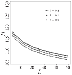
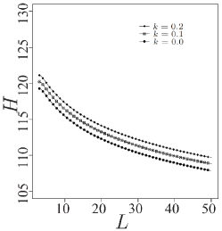
only the diagonal and the upper triangle values are shown. Fig. 1(a) depicts plots of the discussed entropies for $3\leq L\leq 50$, $\beta\in\{0.1,0.5,0.8\}$, and $\boldsymbol{\Sigma}_{U}$. Considering the same interval for the number of looks, Figs. 1(b), 1(c), and 1(d) show the Shannon, Tsallis (of order $\beta=1-10^{-3}$), and Rényi (of order $\beta=0.1$) entropies for the covariance matrix $(1+k)\boldsymbol{\Sigma}_{U}$, $k\in\{0,0.1,0.2\}$, respectively.

(a) $H_{\text{S}}$ and $H^{\beta}_{\text{R}}$ for covariance matrix $\boldsymbol{\Sigma}$

(b) $H_{\text{S}}$ and $(1+k)\boldsymbol{\Sigma}$

(c) $H_{\text{T}}^{1-10^{-3}}$ and $(1+k)\boldsymbol{\Sigma}$

(d) $H_{\text{R}}^{0.1}$ and $(1+k)\boldsymbol{\Sigma}$

(e) $H_{\text{S}}$ and $H_{\text{T}}^{\beta}$ and $\boldsymbol{\Sigma}$

Figure 1: Shannon, Tsallis, and Rényi entropies for several covariance matrices and number of looks.

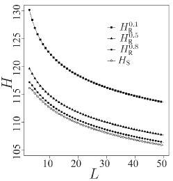
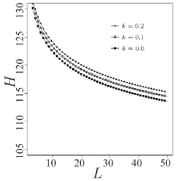
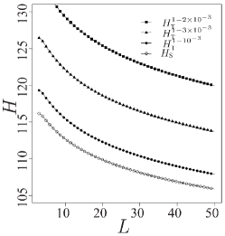
Figs. 1(a) and 1(e) illustrate the property stated in (14). In the case shown here, the convergences are from above, i.e., $H_{\text{S}}$ is always smaller than $H_{\text{R}}^{\beta}$ and $H_{\text{T}}^{\beta}$.

Figs. 1(b) and 1(d) suggest that multiplying the covariance matrix by a constant — hence increasing its determinant — also increases both Shannon and Rényi entropies. As expected, increasing the number of looks leads to smaller entropy values due to the increased SNR.

Although the restricted Tsallis entropy can be used in several fields of image processing [17], the derivation of its variance does not lead to a mathematically tractable expression. Thus, henceforth we focus our attention on the Shannon and Rényi entropies, which allow the necessary algebraic manipulations for the the method described in Section III. In the next section, we derive asymptotic variances for the Shannon and Rényi entropy estimates.

IV-B Asymptotic variances

Let $\boldsymbol{Z}$ be a random matrix which follows a scaled complex Wishart distribution with parameter $\boldsymbol{\theta}$ as already defined. Its log-likelihood is

$$\ell(\boldsymbol{\theta})= mL\ln L+(L-m)\ln|\boldsymbol{Z}|-L\ln|\boldsymbol{\Sigma}|$$

$$-\frac{m(m-1)}{2}\ln\pi-\sum_{k=0}^{m-1}\ln\Gamma(L-k)-L\operatorname{tr}(\boldsymbol{\Sigma}^{-1}\boldsymbol{Z}).$$

Since $\partial\ell(\boldsymbol{\theta})/\partial\operatorname{vec}(\boldsymbol{\Sigma})=\operatorname{vec}(\partial\ell(\boldsymbol{\theta})/\partial\boldsymbol{\Sigma})$ holds true [43], the score functions are given by

$$\ell_{L}=m(\ln L+1)+\ln|\boldsymbol{Z}|-\ln|\boldsymbol{\Sigma}|-\psi_{m}^{(0)}(L)-\operatorname{tr}\big{(}\boldsymbol{\Sigma}^{-1}\boldsymbol{Z}\big{)},$$

and $\ell_{\operatorname{vec}(\Sigma)}=L\operatorname{vec}\big{(}\boldsymbol{\Sigma}^{-1}\boldsymbol{Z}\boldsymbol{\Sigma}^{-1}-\boldsymbol{\Sigma}^{-1}\big{)}$.

The Hessian matrix $\mathcal{J}(\boldsymbol{\theta})$, the Fisher information matrix $\mathcal{K}(\boldsymbol{\theta})$, and the biased version (according to Anfinsen et al. [36]) for Cramér-Rao lower bound $\mathcal{C}(\boldsymbol{\theta})$ are necessary to obtain closed form expressions for the asymptotic entropy variance used in Equation (3). In particular, the following quantity plays a central role:

$$\mathcal{J}_{\Sigma\Sigma}=\frac{\partial}{\partial\operatorname{vec}(\boldsymbol{\Sigma})^{*}}\operatorname{vec}\bigg{(}\frac{\partial\ell(\boldsymbol{\theta})}{\partial\boldsymbol{\Sigma}}\bigg{)}^{t},$$

where $(\cdot)^{*}$ represents complex conjugation. Anfinsen et al. [36] showed that

$$T_{1} =-\frac{\partial(\boldsymbol{\Sigma}^{-1}\boldsymbol{Z}\boldsymbol{\Sigma}^{-1})}{\partial\boldsymbol{\Sigma}}$$

$$=-\boldsymbol{\Sigma}^{-1}\otimes\boldsymbol{\Sigma}^{-1}\boldsymbol{Z}\boldsymbol{\Sigma}^{-1}-\boldsymbol{\Sigma}^{-1}\otimes\boldsymbol{\Sigma}^{-1}\boldsymbol{\Sigma}^{-1}\boldsymbol{Z}.$$

Moreover, it is known that [43]

$$T_{2}=\partial\boldsymbol{\Sigma}^{-1}/\partial\boldsymbol{\Sigma}=-\boldsymbol{\Sigma}^{-1}\otimes\boldsymbol{\Sigma}^{-1}.$$

Thus, we have that

$$\mathcal{J}_{\Sigma\Sigma}= L(T_{2}-T_{1})=L(\boldsymbol{\Sigma}^{-1}\otimes\boldsymbol{\Sigma}^{-1}-\boldsymbol{\Sigma}^{-1}\otimes\boldsymbol{\Sigma}^{-1}\boldsymbol{Z}\boldsymbol{\Sigma}^{-1}$$

$$-\boldsymbol{\Sigma}^{-1}\otimes\boldsymbol{\Sigma}^{-1}\boldsymbol{\Sigma}^{-1}\boldsymbol{Z}).$$ (15)

From Equation (IV-B) we obtain:

$$\mathcal{K}_{\Sigma\Sigma}=\operatorname{E}\{-\mathcal{J}_{\Sigma\Sigma}\}=L\boldsymbol{\Sigma}^{-1}\otimes\boldsymbol{\Sigma}^{-1}.$$ (16)

The analytical expressions for $\mathcal{J}(\boldsymbol{\theta})$, $\mathcal{K}(\boldsymbol{\theta})$, and $\mathcal{C}(\boldsymbol{\theta})$ are, thus,

$$\mathcal{J}(\boldsymbol{\theta})=$$

$$\quad\Bigg{[}\begin{array}[]{cc}\frac{m}{L}-\psi_{m}^{(1)}(L)&\operatorname{vec}(\boldsymbol{\Sigma}^{-1}\boldsymbol{Z}\boldsymbol{\Sigma}^{-1}-\boldsymbol{\Sigma}^{-1})^{t}\\ \operatorname{vec}(\boldsymbol{\Sigma}^{-1}\boldsymbol{Z}\boldsymbol{\Sigma}^{-1}-\boldsymbol{\Sigma}^{-1})^{*}&\mathcal{J}_{\Sigma\Sigma}\end{array}\Bigg{]},$$

$$\mathcal{K}(\boldsymbol{\theta})=\operatorname{E}\{-\mathcal{J}(\boldsymbol{\theta})\}=$$

$$\quad\bigg{[}\begin{array}[]{cc}\psi_{m}^{(1)}(L)-\frac{m}{L}&\operatorname{vec}(\boldsymbol{0}_{m})^{t}\\ \operatorname{vec}(\boldsymbol{0}_{m})&L\boldsymbol{\Sigma}^{-1}\otimes\boldsymbol{\Sigma}^{-1}\end{array}\bigg{]},$$

$$\mathcal{C}(\boldsymbol{\theta})=\mathcal{K}(\boldsymbol{\theta})^{-1}=$$

$$\quad\left[\begin{array}[]{cc}[\psi_{m}^{(1)}(L)-\frac{m}{L}]^{-1}&\operatorname{vec}(\boldsymbol{0}_{m})^{t}\\ \operatorname{vec}(\boldsymbol{0}_{m})&L^{-1}\boldsymbol{\Sigma}\otimes\boldsymbol{\Sigma}\end{array}\right],$$

where $\boldsymbol{0}_{m}$ is the null square matrix of order $m$.

Anfinsen el al. [36] derived the Fisher information matrix for the unscaled complex Wishart law. That approach found that the parameters of such distribution are not orthogonal. Based on $\mathcal{J}(\boldsymbol{\theta})$, we conclude that $L$ and $\boldsymbol{\Sigma}$ become orthogonal under the scaling of the complex Wishart law. Among other benefits, such scaling makes the likelihood equations separable, as shown in the following.

Consider $\{\boldsymbol{Z}_{1},\boldsymbol{Z}_{2},\ldots,\boldsymbol{Z}_{N}\}$ a random sample of size $N$ obtained from $\boldsymbol{Z}\sim\mathcal{W}_{m}(\boldsymbol{\Sigma},L)$. Since $N^{-1}\sum_{k=1}^{N}\nabla\ell_{k}(\widehat{\boldsymbol{\theta}})=\boldsymbol{0}$, we have that

$$\widehat{\boldsymbol{\Sigma}}=\frac{1}{N}\sum_{k=1}^{N}{\boldsymbol{Z}_{k}}=\overline{\boldsymbol{Z}},$$

and

$$m\ln\widehat{L}+\frac{1}{N}\sum_{k=1}^{N}\ln|\boldsymbol{Z}_{k}|-\ln|\overline{\boldsymbol{Z}}|-\psi_{m}^{(0)}(\widehat{L})=0.$$ (17)

Thus, the ML estimator of $\boldsymbol{\Sigma}$ is the sample mean, while $\widehat{L}$ is obtained solving the system shown in Equation (17). The Newton-Raphson iterative method [44] can be used to solve this nonlinear system.

The asymptotic variance given by Equation (3) is determined by $\mathcal{C}(\boldsymbol{\theta})$ and by the term [34]

$$\boldsymbol{\delta}=\biggl{[}\frac{\partial H^{h}_{\phi}(\boldsymbol{\theta})}{\partial L}\;\operatorname{vec}\biggl{(}\frac{H^{h}_{\phi}(\boldsymbol{\theta})}{\partial\boldsymbol{\Sigma}}\biggr{)}^{t}\biggr{]}^{t}.$$

We denote the resulting $\boldsymbol{\delta}$ as $\boldsymbol{\delta}_{\text{S}}$ and $\boldsymbol{\delta}_{\text{R},\beta}$, when $H_{\text{S}}$ and $H^{\beta}_{\text{R}}$ are considered, respectively. We could not find a closed expression for the variance of the restricted Tsallis entropy, so it will not be further considered in the remainder of this work. Analogously, entropy variances are denoted as $\sigma_{\text{S}}^{2}$ and $\sigma_{\text{R},\beta}^{2}$. These quantities are given by expressions (18)-(21).

• Shannon entropy:

  $$\boldsymbol{\delta}_{\text{S}}=\Bigg{[}\begin{array}[]{c}(m-L)\psi_{m}^{(1)}(L)+m-\frac{m^{2}}{L}\\ m\operatorname{vec}\bigl{(}\boldsymbol{\Sigma}^{-1}\bigr{)}\end{array}\Bigg{]}$$ (18)

  and

  $$\sigma_{\text{S}}^{2}=\frac{\bigl{[}(m-L)\psi_{m}^{(1)}(L)+m-\frac{m^{2}}{L}\bigr{]}^{2}}{\psi_{m}^{(1)}(L)-\frac{m}{L}}+\frac{m^{2}}{L}\operatorname{vec}\bigl{(}\boldsymbol{\Sigma}^{-1}\bigr{)}^{t}\bigl{(}\boldsymbol{\Sigma}\otimes\boldsymbol{\Sigma}\bigr{)}\operatorname{vec}\bigl{(}\boldsymbol{\Sigma}^{-1}\bigr{)}.$$ (19)

• Rényi entropy:

  $$\boldsymbol{\delta}_{\text{R},\beta}=\Bigg{[}\begin{array}[]{c}\frac{\beta}{1-\beta}\bigl{[}\psi_{m}^{(0)}(q)-\psi_{m}^{(0)}(L)\bigr{]}-\frac{m\beta\ln(\beta)}{1-\beta}-\frac{m^{2}}{L}\\ m\operatorname{vec}\bigl{(}\boldsymbol{\Sigma}^{-1}\bigr{)}\end{array}\Bigg{]}$$ (20)

  and

  $$\sigma_{\text{R},\beta}^{2}=\frac{\Big{\{}\frac{\beta}{1-\beta}\bigl{[}\psi_{m}^{(0)}(q)-\psi_{m}^{(0)}(L)\bigr{]}-\frac{m\beta\ln(\beta)}{1-\beta}-\frac{m^{2}}{L}\Big{\}}^{2}}{\psi_{m}^{(1)}(L)-\frac{m}{L}}+\frac{m^{2}}{L}\operatorname{vec}\bigl{(}\boldsymbol{\Sigma}^{-1}\bigr{)}^{t}\bigl{(}\boldsymbol{\Sigma}\otimes\boldsymbol{\Sigma}\bigr{)}\operatorname{vec}\bigl{(}\boldsymbol{\Sigma}^{-1}\bigr{)}.$$ (21)

Note that, as expected from Equation (14), $\lim_{\beta\rightarrow 1}\sigma_{\text{R},\beta}^{2}=\sigma_{\text{S}}^{2}.$

The entropies, along with their variances, can be used as alternative goodness-of-fit tests to the one proposed in [45] for the Wishart distribution, specifying $r=1$ in Equation (4). Cintra et al. [19] showed that these statistics outperform the Kolmogorov-Smirnov nonparametric test in intensity SAR imagery. In this paper, we aim to quantify contrast in PolSAR images and situations with $r=2$. In the following, the proposed tests are applied to PolSAR imagery.

V Applications

In this section, we combine the entropies and variances derived in the previous section to form statistical tests, whose performance with respect to test size and power is assessed by Monte Carlo experiments. Finally, the discussed methodology is applied to real data.

V-A Entropy as a feature for discrimination

Fig. 2(a) shows the HH band of a PolSAR L-band image over Weßling, Germany. This image was obtained by the E-SAR sensor [46] with $3.2$ equivalent number of looks (ENL), which is a PolSAR parameter associated to the degree of averaging of SAR measurements during data formation [36]. Three regions were selected: $\text{A}_{1}$, $\text{A}_{2}$, and $\text{A}_{3}$, corresponding to areas with strong, moderate, and weak return, respectively. The image has approximately 3 m resolution.

(a) E-SAR intensity image (HH band)

(b) Data from region $\text{A}_{1}$

(c) Data from region $\text{A}_{2}$

(d) Data from region $\text{A}_{3}$

Figure 2: PolSAR image, selected regions, histograms (dot curve) and fitted scaled complex Wishart distributions: ${\mathcal{W}_{R}}(\widehat{\boldsymbol{\Sigma}},\widehat{L})$ (solid curve) and ${\mathcal{W}}(\widehat{\boldsymbol{\Sigma}},3.2)$ (dashed curve).

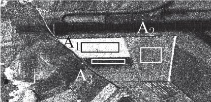
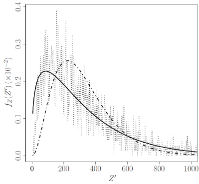
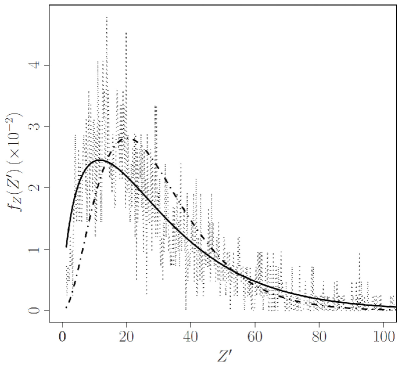
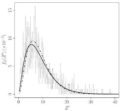
Table II shows the sample size $N$ and the ML estimates of the scaled Wishart distribution parameters for each region. The ENL estimates are close, suggesting similar levels of radar texture in the three regions; such levels are probably low, since the regions appear to be cropland. Notice that the smallest estimated number of looks and the highest value of determinant for the sample convariance matrix belong to region $\text{A}_{1}$, where the texture is more pronounced. Figs. 2(b)-2(d) present histograms and fitted densities from considered data for two distributions of the scaled complex Wishart family: ${\mathcal{W}}(\widehat{\boldsymbol{\Sigma}},3.2)$ and ${\mathcal{W}_{R}}(\widehat{\boldsymbol{\Sigma}},\widehat{L})$. Additionally, Table II also presents the Akaike information criterion (AIC), a measure of the goodness of these fits [47]. In all cases, the ${\mathcal{W}_{R}}$ distribution presented the best fit.

TABLE II: ML estimates for the samples from Figure 2(a) under the relaxed and original Wishart distributions, and their AIC values

Regions	$N$	$|\widehat{\boldsymbol{\Sigma}}|$	$\widehat{L}$	AIC
				${\mathcal{W}}(\widehat{\boldsymbol{\Sigma}},3.2)$	${\mathcal{W}_{R}}(\widehat{\boldsymbol{\Sigma}},\widehat{L})$
$\text{A}_{1}$	3708	355494.500	1.361	50769.93	49856.90
$\text{A}_{2}$	2088	3321.241	1.657	18353.35	17931.51
$\text{A}_{3}$	1079	274.189	2.557	6749.56	6629.15

Table III presents the asymptotic lower and upper bounds for the Shannon and Rényi entropies at the 95% level of confidence, as computed according to Equation (7). The intervals are disjoint, suggesting that the entropy can be used as a feature for region discrimination. The smallest entropies are associated with regions whose estimated covariance matrices have small determinants, in accordance with the case study presented in Section IV-A4.

Noting that (i) the entropy is a measure of randomness, which is associated to variability, and that (ii) PolSAR areas with high reflectance are more affected by speckle noise, even those with negligible texture, it is intuitive that the determinant of the covariance matrix and the entropy are positively correlated. Moreover, the expressions of entropies are also directly proportional to the determinant, i.e., $H_{\text{R}}^{\beta},H_{\text{S}}\propto m\ln|\boldsymbol{\Sigma}|$.

Goodman [48] defined the stochastic covariance matrix determinant as a generalized variance which is associated with the speckle variability, defined as the effect of the speckle noise resulting from multipath interference. Additionally, when there is texture variability it is due to the spatial variability in reflectance, and is associated with the “heterogeneity”, which is the usual measure of the texture level. This last source of variability can be captured by, for instance, the roughness parameter of the polarimetric $\mathcal{G}^{0}$ law [49, 50].

TABLE III: Estimated asymptotic intervals at 95% for the Shannon and Rényi entropies of samples from Figure 2(a)

Region	$\widehat{H_{\text{S}}}$		$\widehat{H_{\text{R}}^{0.1}}$		$\widehat{H_{\text{R}}^{0.8}}$
	Lower	Upper	Lower	Upper	Lower	Upper
$\text{A}_{1}$	37.979	38.432	61.083	61.332	44.045	44.364
$\text{A}_{2}$	30.079	30.541	45.563	45.867	36.124	37.049
$\text{A}_{3}$	19.611	19.949	35.000	35.346	20.901	21.230

V-B Synthetic Data

We quantify the performance of hypothesis tests based on Shannon and Rényi entropies with synthetic data following the scaled complex Wishart distribution, generated as suggested in [51].

The simulation employed the following parameters: (i) $L=3.2$; (ii) the estimated covariance matrices from regions $\text{A}_{1}$, $\text{A}_{2}$, and $\text{A}_{3}$, denoted as $\widetilde{\boldsymbol{\Sigma}}_{1},\widetilde{\boldsymbol{\Sigma}}_{2}$, and $\widetilde{\boldsymbol{\Sigma}}_{3}$, respectively; (iii) sample sizes $N=\{9,49,81,121,400\}$ (i.e., squared windows of side $\{3,7,9,11,20\}$ pixels); and (iv) significance levels $\alpha\in\{1\%,5\%,10\%\}$. After generating two samples of size $N$ from $\boldsymbol{X}\sim\mathcal{W}_{m}(\widetilde{\boldsymbol{\Sigma}}_{i},L)$ and $\boldsymbol{Y}\sim\mathcal{W}_{m}(\widetilde{\boldsymbol{\Sigma}}_{j},L)$, we tested the the null hypothesis $\mathcal{H}_{0}\colon(\widetilde{\boldsymbol{\Sigma}}_{i},L)=(\widetilde{\boldsymbol{\Sigma}}_{j},L)$ for $i,j=1,2,3$. Following [18], we run $5500$ replicas of the Monte Carlo simulation for every case. Empirical test size and power were employed as figures of merit. These quantities are defined as the rejection rates of $\mathcal{H}_{0}$ when this hypothesis is true and is false (i.e., $\boldsymbol{\Sigma}_{i}\neq\boldsymbol{\Sigma}_{j}$), respectively; they are also called Type I error and true positive rates.

Table IV presents the resulting empirical test sizes. From a purely statistical viewpoint, the ideal test is the one whose empirical size is exactly the nominal one for simulated data. Therefore, we conclude that the Rényi entropy for $\beta=0.1$ is generally outperformed by the Shannon and Rényi of order $0.8$, except for $N=9$. The two last hypothesis tests have empirical test sizes close to the nominal levels even for small sample sizes.

TABLE IV: Empirical test sizes based on Shannon and Rényi (of order $0.1$ and $0.8$) entropies for regions A₁, A₂, and A₃ from Figure 2(a); a good test is close to its nominal level.

	$\text{A}_{1}$			$\text{A}_{2}$			$\text{A}_{3}$
$N$	$1\%$	$5\%$	$10\%$	$1\%$	$5\%$	$10\%$	$1\%$	$5\%$	$10\%$
	Shannon entropy
9	1.35	6.15	11.76	1.36	6.16	12.02	1.44	6.20	12.05
49	1.38	5.53	10.44	1.38	5.65	10.35	1.35	5.47	10.44
81	1.33	5.51	9.75	1.35	5.47	9.84	1.35	5.36	10.07
121	1.18	5.56	10.58	1.15	5.51	10.51	1.15	5.49	10.44
400	1.35	5.38	10.33	1.38	5.47	10.40	1.40	5.51	10.22
	Rényi entropy with $\beta=0.8$
9	1.38	6.22	11.65	1.44	6.18	11.93	1.45	6.09	11.78
49	1.27	5.62	10.36	1.31	5.65	10.31	1.33	5.38	10.55
81	1.31	5.47	9.76	1.20	5.47	9.91	1.29	5.36	9.95
121	1.05	5.35	10.45	1.15	5.44	10.44	1.13	5.53	10.55
400	1.35	5.27	10.31	1.36	5.29	10.29	1.27	5.33	10.42
	Rényi entropy with $\beta=0.1$
9	0.69	4.04	8.80	0.76	4.15	8.65	0.82	4.04	8.55
49	0.71	3.62	7.82	0.75	3.87	7.89	0.69	3.45	7.73
81	0.53	3.69	7.51	0.56	3.84	7.49	0.55	3.62	7.51
121	0.60	3.73	7.58	0.60	3.40	7.47	0.53	3.58	7.64
400	0.56	3.84	7.65	0.67	3.82	7.64	0.67	3.62	7.65

Samples from different covariance matrices always led to rejecting the null hypothesis with the proposed statistical tests, thus leading to tests with unitary empirical test power. Table V shows the mean value of the statistics

$$\overline{S}(\text{A}_{i},\text{A}_{j})=\frac{1}{5500}\sum_{k=1}^{5500}S^{h}_{\phi}([\widehat{\boldsymbol{\Sigma}}_{i},\widehat{L}_{i}]_{k},[\widehat{\boldsymbol{\Sigma}}_{j},\widehat{L}_{j}]_{k}),$$

where $S^{h}_{\phi}$ is $S_{\text{S}}$ or $S_{\text{R}}$ as given in (6) and $[\widehat{\boldsymbol{\Sigma}}_{i},\widehat{L}_{i}]_{k}$ are the ML estimates based on generated data from population $A_{i}$ at the $k$th Monte Carlo replica. The table also shows the coefficient of variation (CV) of the test statistics under alternative hypotheses:

$$\operatorname{CV}(\text{A}_{i},\text{A}_{j})=$$

$$\frac{\sqrt{\sum_{k=1}^{5500}[S^{h}_{\phi}([\widehat{\boldsymbol{\Sigma}}_{i},\widehat{L}_{i}]_{k},[\widehat{\boldsymbol{\Sigma}}_{j},\widehat{L}_{j}]_{k})-\overline{S}(\text{A}_{i},\text{A}_{j})]^{2}}}{\overline{S}(\text{A}_{i},\text{A}_{j})\sqrt{5500}}.$$

TABLE V: Mean and coefficient of variation under alternative hypotheses of test statistics based on Shannon and Rényi (of order $0.1$ and $0.8$) entropies

	$\text{A}_{1}$-$\text{A}_{2}$		$\text{A}_{1}$-$\text{A}_{3}$		$\text{A}_{2}$-$\text{A}_{3}$
$N$	$\operatorname{CV}$	$\overline{S}$	$\operatorname{CV}$	$\overline{S}$	$\operatorname{CV}$	$\overline{S}$
	Shannon entropy
9	20.59	108.16	13.83	248.53	38.42	29.89
49	8.65	576.23	5.82	1329.19	16.38	156.21
81	6.70	949.51	4.52	2191.84	12.71	256.54
121	5.51	1418.22	3.71	3274.03	10.43	383.17
400	3.01	4687.29	2.02	10817.80	5.72	1265.69
	Rényi entropy with $\beta=0.8$
9	20.56	106.72	13.72	245.22	38.45	29.50
49	8.63	569.69	5.76	1314.11	16.40	154.43
81	6.67	938.93	4.47	2167.39	12.72	253.68
121	5.48	1402.43	3.66	3237.61	10.42	378.93
400	3.00	4635.65	2.00	10698.61	5.71	1251.74
	Rényi entropy with $\beta=0.1$
9	21.70	78.42	14.27	180.12	40.60	21.79
49	9.11	423.29	6.00	976.32	17.44	114.77
81	7.02	698.47	4.63	1612.06	13.50	188.81
121	5.73	1043.26	3.77	2408.63	11.00	282.06
400	3.15	3450.84	2.07	7963.98	6.03	931.79

The largest means $\overline{S}(\text{A}_{i},\text{A}_{j})$ correspond to the largest absolute values $\operatorname{abs}(|\widetilde{\boldsymbol{\Sigma}}_{i}|-|\widetilde{\boldsymbol{\Sigma}}_{j}|)$, leading to the following relations:

$$\overline{S}(\text{A}_{1},\text{A}_{3})>\overline{S}(\text{A}_{1},\text{A}_{2})>\overline{S}(\text{A}_{2},\text{A}_{3}).$$ (22)

Shannon test statistics produced the largest test statistics when contrasting samples from different areas.

V-C Real Data

Applying the methodology described above to real data, we obtained the results shown in Fig. 3. To that end, the following steps were followed:

1:for $j=1,2,\ldots,5500$ do

2:      Extract two regions $\boldsymbol{U}_{j}$ and $\boldsymbol{V}_{j}$ from areas $\text{A}_{1},\text{A}_{2},\text{ and }\text{A}_{3}$.

3:     By sampling without replacement, generate two $N$-point vectors $\boldsymbol{u}^{(j)}$ and $\boldsymbol{v}^{(j)}$ from $\boldsymbol{U}_{j}$ and $\boldsymbol{V}_{j}$, respectively, granting $\boldsymbol{u}^{(i)}\neq\boldsymbol{u}^{(j)}$ and $\boldsymbol{v}^{(i)}\neq\boldsymbol{v}^{(j)}$ for $i\neq j$.

4:     Estimate the parameter vectors $\widehat{\boldsymbol{\theta}}^{(j)}_{1}$ and $\widehat{\boldsymbol{\theta}}^{(j)}_{2}$ based on $\boldsymbol{u}^{(j)}$ and $\boldsymbol{v}^{(j)}$, respectively.

5:      Compute the decision from Proposition 1 for $\alpha=\{1\%,5\%,10\%\}$.

6:end for

7: Let $T$ be the number of times that the null hypothesis is rejected. Calculate the empirical test size ($\widehat{\alpha}_{1-\alpha}$) and power ($1-\widehat{\beta}_{1-\alpha}$) at level $\alpha$ as

$$\left\{\begin{array}[]{c}\widehat{\alpha}_{1-\alpha}=T/5500,\text{ if }\boldsymbol{V}_{j}=\boldsymbol{U}_{j},\\ 1-\widehat{\beta}_{1-\alpha}=T/5500,\text{ if }\boldsymbol{V}_{j}\neq\boldsymbol{U}_{j},\end{array}\right.$$

where $\widehat{\beta}_{1-\alpha}$ is the Type II error rate; i.e., the estimate for the probability of not rejection of $\mathcal{H}_{0}$ when the null hypothesis is false. We considered $N$ the number of observations in squared windows of size $\{3\times 3,4\times 4,\ldots,23\times 23\}$.

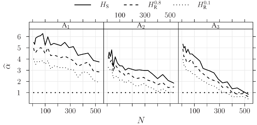
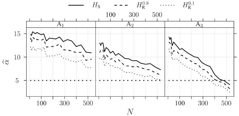
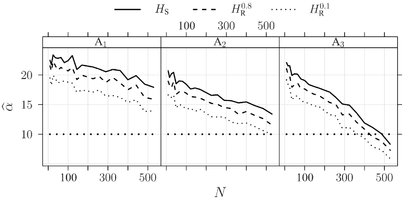
Fig. 3 shows the empirical test sizes, with the nominal test size $\alpha$ in dotted line. The behavior of $\widehat{\alpha}_{1-\alpha}$ is consistent across the three values of $\alpha$: the empirical test size is larger in Shannon than in Rényi $\beta=0.8$ which, in turn, is larger than Rényi $\beta=0.1$. The fastest convergence to $\alpha$ with respect to the sample size is consistently observed in area $\text{A}_{3}$. No test attains the nominal size in area $\text{A}_{1}$. This is probably due to its pronounced brightness and roughness, as noted in Table II.

(a) Size $1\%$

(b) Size $5\%$

(c) Size $10\%$

Figure 3: Empirical test size for different regions at several sample sizes and nominal levels.

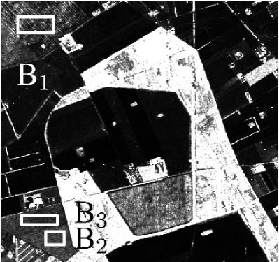
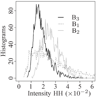
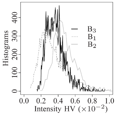
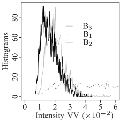
In the following we select visually similar regions, but with distinct statistical properties. To that end, Fig. 4(a) shows an EMISAR image of Foulum (Denmark) obtained with eight nominal looks over agricultural areas and sub 10 m resolution; three regions were selected for our study. Table VI presents the sample sizes and the ML estimates, while Figs. 4(b), 4(c) and 4(d) show empirical densities of different areas and channels. The empirical densities of B₂ and B₃ are the closest for all polarization channels, as well as their estimates of $L$.

(a) EMISAR Image

(b) HH Channel

(c) HV Channel

(d) VV Channel

Figure 4: PolSAR image, selected regions and their empirical densities in all polarizations.

TABLE VI: ML estimates for the samples from Figure 4(a)

Regions	$N$	$|\widehat{\boldsymbol{\Sigma}}|$	$\widehat{L}$
$\text{B}_{1}$	3192	$1.609\times 10^{-5}$	6.925
$\text{B}_{2}$	1408	$1.112\times 10^{-6}$	11.937
$\text{B}_{3}$	1848	$5.814\times 10^{-7}$	10.752

We quantify the discrimination between selected regions by means of $S_{\text{S}}$ and $S_{\text{R}}^{0.1}$ performing steps 1–7 with the Foulum samples. Since Rényi entropy converges to Shannon when the order tends to $1$, we omit the analysis of $S_{\text{R}}^{0.8}$ because it is similar to $S_{\text{S}}$, as illustrated in Fig. 5.

Figure 5: Empirical test power at the level $10\%$.

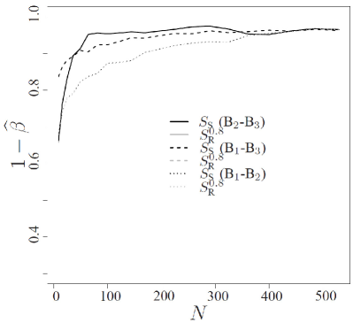
Figs. 6(a), 6(b) and 6(c) exhibit the empirical test power. In general terms, the estimated power increase quickly when sample sizes increase. The test based on the Shannon entropy outperforms the one based on Rényi’s.

(a) 1%

(b) 5%

(c) 10%

Figure 6: Empirical test power for different regions at several sample sizes and nominal levels; a good test has high power in these cases.

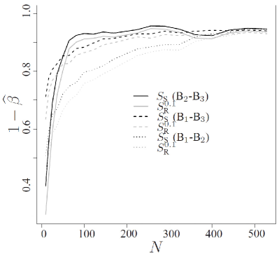
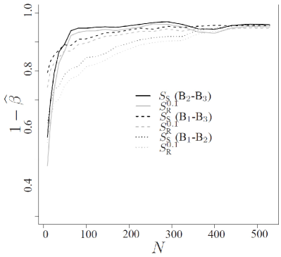
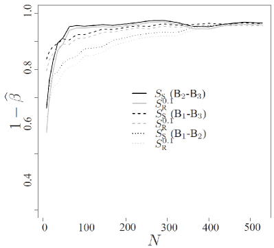
These results suggest that the test statistics in terms of the Shannon entropy is a more appropriate tool for change and boundary detection in PolSAR images than the measure based on the Rényi entropy.

VI Conclusions

In this paper, the closed expressions for Shannon, Rényi, and Tsallis entropies have been derived for data distributed according with the scaled complex Wishart distribution. The variances of the two first entropies were also derived when parameters are replaced by ML estimators, leading to the derivation of two test statistics with known asymptotic distributions. The statistics based on the Tsallis entropy were not derived since its variance could not be expressed in closed form.

New hypothesis tests and confidence intervals based on the ($h,\phi$)-family of entropies were derived for the scaled complex Wishart distribution. These new statistical tools provide means for contrasting $r\geq 2$ samples and verifying if they come from the same distribution. Such tools were derived by obtaining orthogonal maximum likelihood estimators for the scaled complex Wishart law, and by characterizing their asymptotic behavior.

Monte Carlo experiments were employed for quantifying the performance of the proposed hypotheses tests. The results provided evidence that the statistic based on the Shannon entropy is the most efficient in terms of empirical test size and power.

An application to actual data was also considered in order to assess the performance of the proposed hypothesis tests. The empirical test sizes observed with real data are relatively high when dealing with small samples, but they decrease as the sample size increases. As expected, the tests presented the worst results in the most heterogeneous situations. Nevertheless, they perform correctly when the sample size is increased.

The hypothesis test based on the Shannon entropy presented the smallest empirical test size. All test statistics detected differences among different regions at the specified levels. This is important for PolSAR image analysis, such as in boundary detection [22] and change detection [24].

As an overall conclusion, the Shannon entropy can be safely used for discriminating areas in PolSAR imagery. Moreover, the Shannon entropy it is not challenged in terms of simplicity either, which consolidates its position as the preferred entropy measure. However, care must be taken when small samples are analyzed. Indeed, in this case, the proposed tests are prone to classifying regions of similar natures as distinct, i.e., to incurring in Type I error. In practice, however, this issue is not severe, since PolSAR image processing often handles data with a large number of pixels.

Further research will consider models which include heterogeneity [49, 50, 22], robust, improved and nonparametric inference [52, 53, 54, 55], and small samples issues [56].

Alejandro C. Frery graduated in Electronic and Electrical Engineering from the Universidad de Mendoza, Argentina. His M.Sc. degree was in Applied Mathematics (Statistics) from the Instituto de Matemática Pura e Aplicada (Rio de Janeiro) and his Ph.D. degree was in Applied Computing from the Instituto Nacional de Pesquisas Espaciais (São José dos Campos, Brazil). He is currently with the Instituto de Computação, Universidade Federal de Alagoas, Maceió, Brazil. His research interests are statistical computing and stochastic modelling.

Renato J. Cintra earned his B.Sc., M.Sc., and D.Sc. degrees in Electrical Engineering from Universidade Federal de Pernambuco, Brazil, in 1999, 2001, and 2005, respectively. In 2005, he joined the Department of Statistics at UFPE. During 2008-2009, he worked at the University of Calgary, Canada, as a visiting research fellow. He is also a graduate faculty member of the Department of Electrical and Computer Engineering, University of Akron, OH. His long term topics of research include theory and methods for digital signal processing, communications systems, and applied mathematics.

Abraão D. C. Nascimento holds B.Sc.  M.Sc.  and D.Sc. degrees in Statistics from Universidade Federal de Pernambuco (UFPE), Brazil, in 2005, 2007, and 2012, respectively. In 2012, he joined the Department of Statistics at UFPE as Substitute Professor. His research interests are statistical information theory, inference on random matrices, and asymptotic theory.

References

- [1] J. S. Lee and E. Pottier, Polarimetric Radar Imaging: From Basics to Applications. Boca Raton: CRC, 2009.
- [2] F. T. Ulaby and C. Elachi, Radar Polarimetriy for Geoscience Applications. Norwood: Artech House, 1990.
- [3] J. M. Beaulieu and R. Touzi, “Segmentation of textured polarimetric SAR scenes by likelihood approximation,” IEEE Transactions on Geoscience and Remote Sensing, vol. 42, no. 10, pp. 2063–2072, 2004.
- [4] P. R. Kersten, J. S. Lee, and T. L. Ainsworth, “Unsupervised classification of polarimetric synthetic aperture radar images using fuzzy clustering and EM clustering,” IEEE Transactions on Geoscience and Remote Sensing, vol. 43, no. 3, pp. 519–527, 2005.
- [5] J. Schou, H. Skriver, A. H. Nielsen, and K. Conradsen, “CFAR edge detector for polarimetric SAR images,” IEEE Transactions on Geoscience and Remote Sensing, vol. 41, no. 1, pp. 20–32, 2003.
- [6] C. E. Shannon, “A mathematical theory of communication,” Bell System Technical Journal, vol. 27, pp. 379–423, July 1948.
- [7] S. Nadarajah and K. Zografos, “Formulas for Rényi information and related measures for univariate distributions,” Information Science, vol. 155, pp. 119–138, 2003.
- [8] ——, “Expressions for Rényi and Shannon entropies for bivariate distributions,” Information Sciences, vol. 170, no. 2-4, pp. 173–189, 2005.
- [9] K. Zografos and S. Nadarajah, “Expressions for Rényi and Shannon entropies for multivariate distributions,” Statistics & Probability Letters, vol. 71, no. 1, pp. 71–84, 2005.
- [10] K. S. Song, “Rényi information, log-likelihood and an intrinsic distribution measure,” Journal of Statistical Planning and Inference, vol. 93, pp. 51–69, 2001.
- [11] M. Basseville, “Distance measures for signal processing and pattern recognition,” Signal Processing, vol. 18, pp. 349–369, 1989.
- [12] S. J. Maybank, “Application of the Fisher-Rao metric to ellipse detection,” International Journal of Computer Vision, vol. 72, no. 3, pp. 287–307, 2007.
- [13] M. Liuni, A. Robel, M. Romito, and X. Rodet, “Rényi information measures for spectral change detection,” in IEEE International Conference on Acoustics, Speech and Signal Processing (ICASSP’2011), May 2011, pp. 3824–3827.
- [14] C. Tsallis, “Possible generalization of Boltzmann–Gibbs statistics,” Journal of Statistical Physics, vol. 52, pp. 479–487, 1988.
- [15] ——, “Entropic nonextensivity: a possible measure of complexity,” Chaos, Solitons, & Fractals, vol. 13, pp. 371–391, 2002.
- [16] G. Wilk and Z. Wlodarczyk, “Example of a possible interpretation of Tsallis entropy,” Physica A: Statistical Mechanics and its Applications, vol. 387, no. 19-20, pp. 4809–4813, 2008.
- [17] J. Morio, P. Réfrégier, F. Goudail, P. C. Dubois Fernandez, and X. Dupuis, “A characterization of Shannon entropy and Bhattacharyya measure of contrast in polarimetric and interferometric SAR image,” Proceedings of the IEEE (PIEEE), vol. 97, no. 6, pp. 1097–1108, June 2009.
- [18] A. D. C. Nascimento, R. J. Cintra, and A. C. Frery, “Hypothesis testing in speckled data with stochastic distances,” IEEE Transactions on Geoscience and Remote Sensing, vol. 48, no. 1, pp. 373–385, 2010.
- [19] R. J. Cintra, A. C. Frery, and A. D. C. Nascimento, “Parametric and nonparametric tests for speckled imagery,” Pattern Analysis and Applications, in press.
- [20] A. C. Frery, A. D. C. Nascimento, and R. J. Cintra, “Information theory and image understanding: An application to polarimetric SAR imagery,” Chilean Journal of Statistics, vol. 2, no. 2, pp. 81–100, 2011.
- [21] M. Salicrú, M. L. Mendéndez, and L. Pardo, “Asymptotic distribution of ()-entropy,” Communications in Statistics - Theory Methods, vol. 22, no. 7, pp. 2015–2031, 1993.
- [22] A. C. Frery, J. Jacobo-Berlles, J. Gambini, and M. Mejail, “Polarimetric SAR image segmentation with B-splines and a new statistical model,” Multidimensional Systems and Signal Processing, vol. 21, pp. 319–342, 2010.
- [23] J. Gambini, M. Mejail, J. Jacobo-Berlles, and A. C. Frery, “Accuracy of edge detection methods with local information in speckled imagery,” Statistics and Computing, vol. 18, no. 1, pp. 15–26, 2008.
- [24] J. Inglada and G. Mercier, “A new statistical similarity measure for change detection in multitemporal SAR images and its extension to multiscale change analysis,” IEEE Transactions on Geoscience and Remote Sensing, vol. 45, no. 5, pp. 1432–1445, 2007.
- [25] K. Conradsen, A. A. Nielsen, J. Schou, and H. Skriver, “A test statistic in the complex Wishart distribution and its application to change detection in polarimetric SAR data,” IEEE Transactions on Geoscience and Remote Sensing, vol. 41, no. 1, pp. 4–19, 2003.
- [26] C. Lopez-Martinez and X. Fabregas, “Polarimetric SAR speckle noise model,” IEEE Transactions on Geoscience and Remote Sensing, vol. 41, no. 10, pp. 2232–2242, 2003.
- [27] F. Goudail and P. Réfrégier, “Contrast definition for optical coherent polarimetric images,” IEEE Transactions on Pattern Analysis and Machine Intelligence, vol. 26, no. 7, pp. 947–951, July 2004.
- [28] N. R. Goodman, “Statistical analysis based on a certain complex Gaussian distribution (an introduction),” The Annals of Mathematical Statistics, vol. 34, pp. 152–177, 1963.
- [29] D. Blatt and A. O. Hero, “On tests for global maximum of the log-likelihood function,” IEEE Transactions on Information Theory, vol. 53, pp. 2510–2525, July 2007.
- [30] D. L. Donoho, M. Vetterli, R. A. DeVore, and I. Daubechies, “Data compression and harmonic analysis,” IEEE Transactions on Information Theory, vol. 44, no. 6, pp. 2435–2476, October 1998.
- [31] S. Kullback, Information Theory and Statistics. Dover, 1978.
- [32] J. Havrda and F. Chalvat, “Concept of structural -entropy,” Kybernetika, vol. 3, pp. 30–35, 1967.
- [33] A. Rényi, “On measures of entropy and information,” in 4th Berkeley Symposium on Mathematical Statistics and Probability, vol. 1, 1961, pp. 547–561.
- [34] L. Pardo, D. Morales, M. Salicrú, and M. L. Menéndez, “Large sample behavior of entropy measures when parameters are estimated,” Communications in Statistics - Theory and Methods, vol. 26, no. 2, pp. 483–501, 1997.
- [35] W. G. Cochran, “The distribution of quadratic forms in a normal system, with applications to the analysis of covariance,” Mathematical Proceedings of the Cambridge Philosophical Society, vol. 30, no. 2, pp. 178–191, 1934.
- [36] S. N. Anfinsen, A. P. Doulgeris, and T. Eltoft, “Estimation of the equivalent number of looks in polarimetric synthetic aperture radar imagery,” IEEE Transactions on Geoscience and Remote Sensing, vol. 47, no. 11, pp. 3795–3809, 2009.
- [37] S. N. Anfinsen and T. Eltoft, “Application of the matrix-variate Mellin transform to analysis of polarimetric radar images,” IEEE Transactions on Geoscience and Remote Sensing, vol. 49, no. 6, pp. 2281–2295, June 2011.
- [38] T. M. Cover and J. A. Thomas, Elements of Information Theory. New York: Wiley-Interscience, 1991.
- [39] D. Jiulin, “Property of Tsallis entropy and principle of entropy increase,” Bulletin of the Astronomical Society of India, vol. 35, pp. 691–696, 2010.
- [40] K. V. Mardia, J. M. Bibby, and J. T. Kent, Multivariate analysis, ser. Probability and mathematical statistics. Academic Press, 1982.
- [41] S. R. Cloude and E. Pottier, “An entropy based classification scheme for land application of polarimetric SAR,” IEEE Transactions on Geoscience and Remote Sensing, vol. 35, pp. 68–78, 1997.
- [42] W. Yan, W. Yang, Y. Liu, and H. Sun, “Unsupervised classification of PolinSAR image based on Shannon entropy characterization,” in Proceedings of the 2010 IEEE International Conference on Signal Processing (ICSP 2010), October 2010, pp. 2192 –2195.
- [43] A. Hjorungnes and D. Gesbert, “Complex-valued matrix differentiation: Techniques and key results,” IEEE Transactions on Signal Processing, vol. 55, no. 6, pp. 2740–2746, June 2007.
- [44] J. E. Gentle, Elements of Computational Statistics, ser. Statistics and computing. Springer, 2002.
- [45] S. N. Anfinsen, A. P. Doulgeris, and T. Eltoft, “Goodness-of-fit tests for multilook polarimetric radar data based on the Mellin transform,” IEEE Transactions on Geoscience and Remote Sensing, vol. 49, no. 7, pp. 2764 –2781, July 2011.
- [46] R. Horn, “The DLR airborne SAR project E-SAR,” in Geoscience and Remote Sensing Symposium, vol. 3. IEEE Press, 1996, pp. 1624–1628.
- [47] A. K. Seghouane and S. I. Amari, “The AIC criterion and symmetrizing the Kullback-Leibler divergence,” IEEE Transactions on Neural Networks, vol. 18, no. 1, pp. 97–106, 2007.
- [48] N. R. Goodman, “The distribution of determinant of a complex Wishart distributed matrix,” The Annals of Mathematical Statistics, vol. 34, pp. 178–180, 1963.
- [49] C. C. Freitas, A. C. Frery, and A. H. Correia, “The polarimetric distribution for SAR data analysis,” Environmetrics, vol. 16, no. 1, pp. 13–31, 2005.
- [50] A. C. Frery, A. H. Correia, and C. C. Freitas, “Classifying multifrequency fully polarimetric imagery with multiple sources of statistical evidence and contextual information,” IEEE Transactions on Geoscience and Remote Sensing, vol. 45, pp. 3098–3109, 2007.
- [51] J. S. Lee, M. R. Grunes, and R. Kwok, “Classification of multi-look polarimetric SAR imagery based on complex Wishart distribution,” International Journal of Remote Sensing, vol. 15, no. 11, pp. 2299–2311, September 1994.
- [52] H. Allende, A. C. Frery, J. Galbiati, and L. Pizarro, “M-estimators with asymmetric influence functions: the GA0 distribution case,” Journal of Statistical Computation and Simulation, vol. 76, no. 11, pp. 941–956, 2006.
- [53] E. Giron, A. C. Frery, and F. Cribari-Neto, “Nonparametric edge detection in speckled imagery,” Mathematics and Computers in Simulation, vol. 82, pp. 2182–2198, 2012.
- [54] M. Silva, F. Cribari-Neto, and A. C. Frery, “Improved likelihood inference for the roughness parameter of the GA0 distribution,” Environmetrics, vol. 19, no. 4, pp. 347–368, 2008.
- [55] K. L. P. Vasconcellos, A. C. Frery, and L. B. Silva, “Improving estimation in speckled imagery,” Computational Statistics, vol. 20, no. 3, pp. 503–519, 2005.
- [56] A. C. Frery, F. Cribari-Neto, and M. O. Souza, “Analysis of minute features in speckled imagery with maximum likelihood estimation,” EURASIP Journal on Applied Signal Processing, vol. 2004, no. 16, pp. 2476–2491, 2004.
![[Uncaptioned image]](/html/1210.4154/assets/x21.png) |