New developments in PJFry

Abstract:

We report on recent progress in numerical evaluation of one loop tensor integrals. A public C++ package PJFry [1, 2] implementing algorithms from Ref. [3] and its extension to hexagons up to rank 6 are presented.

1 Introduction

The stable numerical evaluation of tensor integrals is one of the central ingredients of one loop Feynman diagram calculations. It can also be efficiently applied in modern techniques like tensorial reconstruction at integrand level [4] or the Open Loops method [5].

The classic Passarino-Veltman reduction scheme allows to express tensor integrals in terms of a basis of (4-2$\epsilon$)-dimensional scalar 1-, 2-, 3- and 4-point integrals with kinematic coefficients [6, 7, 8]. While it works well for processes with up to 4 external states, for 5 and more legs the numerical stability of the reduction coefficients is spoiled by the appearance of inverse Gram determinants. A number of methods have been proposed to avoid inverse Gram determinants and to improve the numerical stability [9, 10, 11, 12, 13, 14, 15, 16, 3].

In this contribution we introduce the open-source tensor reduction package PJFry which avoids Gram determinant instability problems by using dimensional recurrence-based algorithms developed in [1, 2, 3, 14, 15, 16, 17, 18, 19, 20, 21, 22].

2 The reduction algorithm

We define dimensionally regulated n-point 1-loop tensor integral of rank R as

$$I_{n}^{\mu_{1}\dotsc\mu_{R}}=(2\pi\mu)^{2\epsilon}\int\frac{d^{d}k}{i\pi^{d/2}}\frac{k^{\mu_{1}}\dotsm k^{\mu_{R}}}{\left((k{-}q_{1})^{2}-m_{1}^{2}+i\epsilon\right)\dotsm\left((k{-}q_{n})^{2}-m_{n}^{2}+i\epsilon\right)}$$ (1)

where the chords $$q_{i}$$ are defined by the external momenta, see Fig. 2:

$$q_{1}=p_{1},\;q_{2}=p_{1}+p_{2},\;q_{3}=p_{1}+p_{2}+p_{3},\;\dotsc,\;q_{n}=\sum_{i=1}^{n}p_{i}$$ (2)

Any one loop tensor integral can be rewritten in terms of scalar tensor form-factors separating the Lorentz structure into products of external momenta and metric tensors:

$$I_{n}^{\mu_{1}\dotsc\mu_{R}}=\sum_{i_{1},\dotsc,i_{R}}^{n}q_{i_{1}}^{[\mu_{1}}\dotsm q_{i_{R}}^{\mu_{R}]}F^{(n)}_{i_{1}\dotsc i_{R}}+\sum_{i_{3},\dotsc,i_{R}}^{n}{g\mathstrut}^{[\mu_{1}\mu_{2}}q_{i_{3}}^{\mu_{3}}\dotsm q_{i_{R}}^{\mu_{R}]}F^{(n)}_{00i_{3}\dotsc i_{R}}+\dotsb$$ (3)

where square brackets denote non-equivalent symmetrization, which gives the set of all non-equivalent permutations.

Following Ref. [18] tensor form-factors can be mapped to scalar integrals in higher dimension and shifted powers of denominators:

$$F^{(n)}_{i} =-I_{n,i}^{[2]}, F^{(n)}_{ij} =n_{ij}I_{n,ij}^{[4]}, F^{(n)}_{00} =-\frac{1}{2}I_{n}^{[2]}, F^{(n)}_{ijk} =-n_{ijk}I_{n,ijk}^{[6]}, F^{(n)}_{00k} =\frac{1}{2}I_{n,k}^{[4]}.$$ (4)

where $I_{n,i_{1}i_{2}\dotsc}^{[2l],s_{1}s_{2}\dotsc}$ is a generalized scalar loop integral in shifted dimension:

$$I_{n,i_{1}i_{2}\dotsc}^{[2l],s_{1}s_{2}\dotsc}=(2\pi\mu)^{2\epsilon}\int\frac{d^{d+2l}k}{i\pi^{d/2+l}}\prod_{r=1}^{n}\frac{1}{\left((k-q_{r})^{2}-m_{r}^{2}+i\epsilon\right)^{1+\delta_{ri_{1}}+\delta_{ri_{2}}+\dotsb-\delta_{rs_{1}}-\delta_{rs_{2}}-\dotsb}}$$ (5)

The symbols $n_{i_{1}i_{2}\dotsc}$ in (4) are shorthand notations for combinatorial factors introduced in [16].

Now one can use dimensional recurrence relations derived in Ref. [19, 20] to express tensor form-factors in terms of (4-2$\epsilon$)-dimensional scalar integrals:

$$()_{n}(d+2l-\sum_{i=1}^{n}\nu_{i}+1)I_{n}^{[2(l+1)]} =\biggl{(}\begin{matrix}0\\ 0\end{matrix}\biggr{)}_{\!n}I_{n}^{[2l]}-\sum_{s=1}^{n}\biggl{(}\begin{matrix}0\\ s\end{matrix}\biggr{)}_{\!n}\mathbf{s}^{-}I_{n}^{[2l]}$$ (6)

$$()_{n}v_{j}\>\mathbf{j}^{+}I_{n}^{[2(l+1)]} =-\biggl{(}\begin{matrix}j\\ 0\end{matrix}\biggr{)}_{\!n}I_{n}^{[2l]}+\sum_{s=1}^{n}\biggl{(}\begin{matrix}j\\ s\end{matrix}\biggr{)}_{\!n}\mathbf{s}^{-}I_{n}^{[2l]}$$ (7)

where $\mathbf{s}^{-}$ is $s^{\text{th}}$ denominator power lowering operator, $\mathbf{j}^{+}$ is $j^{\text{th}}$ denominator power raising operator and $\nu_{j}$ is the power of the $j^{\text{th}}$ denominator.

However the direct application of eqs. (6) and (7) introduces inverse Gram determinants $()_{n}$ which will spoil numerical accuracy in large regions of the physical phase space.

The problem of inverse 5-point Gram determinants has been addressed, among others, in [3] where expressions for tensor pentagons have been derived using signed minor algebraic relations.

Figure 1: Basis integrals for the tensor reduction of pentagons

The basis shown in Fig. 1 can be further reduced using an additional recurrence relation:

$$\biggl{(}\begin{matrix}0\\ 0\end{matrix}\biggr{)}_{\!n}v_{j}\>\mathbf{j}^{+}I_{n}^{[2(l+1)]} =-\biggl{(}\begin{matrix}j\\ 0\end{matrix}\biggr{)}_{\!n}(d+2l-\sum_{i=1}^{n}\nu_{i}+1)I_{n}^{[2(l+1)]}+\sum_{s=1}^{n}\biggl{(}\begin{matrix}0s\\ 0j\end{matrix}\biggr{)}_{\!n}\mathbf{s}^{-}I_{n}^{[2l]}.$$ (8)

With the help of the above relation one can reduce powers of all denominators to $1$ without introduction of inverse Gram determinants, however it does not reduce the dimension. Thus we cannot recurse all the way down to standard (4-2$\epsilon$)-dimensional scalar integrals and we have to extend our integral basis:

$$I_{4}^{[8],s}, I_{4}^{[6],s}, I_{4}^{[4],s}, I_{4}^{[2],s}, I_{3}^{[8],st}, I_{3}^{[6],st}, I_{3}^{[4],st}, I_{3}^{[2],st}.$$ (9)

For the numerical evaluation of these additional integrals (9) we employ a series expansion in the small Gram region [3]. This method treats all mass-kinematic combinations uniformly with dimensional recurrence, therefore works equally well for both massive and massless cases.

Our expansion formula is easily derived from (6), which can be written in the following form:

$${X}(d+2l-n+1)I_{n}^{[2(l+1)]}=I_{n}^{[2l]}-Z_{n}^{[2l]},\qquad{X}=\frac{()_{n}}{\binom{0}{0}_{n}},\qquad Z_{n}^{[2l]}=\sum_{s=1}^{n}\frac{\binom{s}{0}_{n}}{\binom{0}{0}_{n}}I_{n}^{[2l],s}.$$ (10)

solving the recurrence we get

$${I_{n}^{[2l]}}=\sum_{m=0}^{M}a_{m}^{(l)}{X^{m}}{Z_{n}^{[2(l+m)]}}+\Bigl{[}a_{M}^{(l)}X^{M}I_{n}^{[2(l+M)}\Bigr{]},\qquad a_{m}^{(l)}=2^{m}\left(\!\frac{d+2l-n+1}{2}\!\right)_{\!m}$$ (11)

where $(a)_{m}=\Gamma(m+a)/\Gamma(a)$ is the Pochhammer symbol.

3 The PJFry reduction library

The PJFry package [1, 2] is an open source library for the numerical evaluation of one loop tensor integrals. Is is licensed under the GNU Lesser General Public License. The latest version can be obtained from the program webpage at https://github.com/Vayu/PJFry/.

The program needs an external library for the evaluation of (4-2$\epsilon$)-dimensional scalar integrals. Currently QCDLoop [23] and OneLOop [24] are supported. The tensor reduction formulae of the PJFry package rely essentially on Ref. [3], where the dimensional recurrence algorithms developed in Refs. [19, 20] were explored. Due to the recursive nature of the numerical algorithms in PJFry, one can greatly benefit from reusing building blocks throughout the calculation.

The main features of the current public version are:

• Reduction of up to rank 5 pentagon tensor integrals

• Any combination of real internal or external masses

• Leading Gram determinants are avoided by the reduction procedure

• Subleading small Gram determinants are treated with asymptotic expansions

• A cache system gives lower point tensor integrals at no extra cost

• Interfaces for C, FORTRAN, C++, Mathematica and GoSam [25].

The different algorithms used in the program are schematically illustrated for tensor pentagon form factors of ranks 2 and 3 in Fig. 3. The blue lines correspond to the reduction formulae of [3]. In the reduction of 4-point functions teal lines represent direct downward recursions for large Gram determinant (6), while the solid red paths represent an alternative scheme with Cayley determinants (8). Relations which are shared by both schemes are drawn with two-colored dashed lines. The small Gram series expansion procedure (11) is depicted for boxes by dotted red lines. Similarly for 3-point functions we use green lines for (6), solid magenta lines for (8) of $I_{3,i}^{[2]}$ and dotted magenta lines for the series expansions of scalar $I_{3}^{[2l]}$ in the small Gram case.

Due to the 4-dimensionality of space-time the problem of inverse Gram determinants does not appear beyond the 5-point case. Therefore after establishing stable numerical methods for the evaluation of pentagons we can use them to construct higher point functions without additional effort.

In PJFry we implemented a well known expression [14, 15, 20, 21, 22, 26] for tensor hexagons up to rank 6 written in terms of pentagons up to rank 5:

$$I_{6}^{\mu_{1}\ldots\mu_{R-1}\mu_{R}}=-\sum^{6}_{s=1}I_{5}^{\mu_{1}\ldots\mu_{R-1},s}\sum_{i=1}^{6}q_{i}^{\mu_{R}}\frac{\binom{0s}{0i}_{6}}{\binom{0}{0}_{6}}$$ (12)

Similar representations exist also for 7 and 8-point functions [27, 28]. For higher point functions one might consider using optimized expressions based on contracted tensors [29].

In addition to six point functions the upcoming version of PJFry supports complex internal masses and extended precision via the qd library [30]. Both options are available only if using OneLOop [24].

The installation is done via a configure script. See the INSTALL file for a detailed description of available options.

The Mathematica interface follows the conventions of LoopTools [31] (see Fig. 2) and can be called from a Mathematica session:

In:=   Install["PJFry"]
Out:=  PJFry MathLink
Out:=  Type Names["PJFry‘*"] to show exported names

The list of exported functions can be obtained by typing

In:=   Names["PJFry‘*"]
Out:=  {"A0v0", "B0v0", "B0v1", "B0v2", "C0v0", "C0v1", "C0v2",
        "C0v3", "ClearCache", "D0v0", "D0v1", "D0v2", "D0v3",
        "D0v4", "E0v0", "E0v1", "E0v2", "E0v3", "E0v4", "E0v5",
        "F0v0", "F0v1", "F0v2", "F0v3", "F0v4", "F0v5", "F0v6",
        "GetMu2", "SetMu2"}

All functions have a short help message which can be accessed by prepending the function name in a call with a question mark (e.g. ?F0v1).

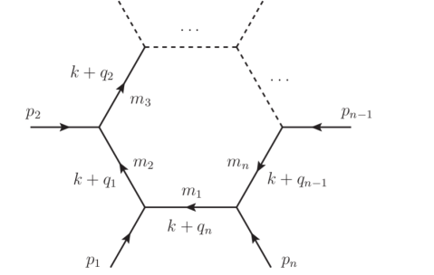
Figure 2: Momenta labeling

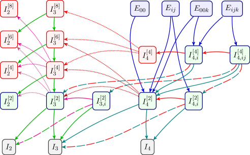
Figure 3: Rank 2 and 3 pentagon form-factors calculation flowchart

As an example we demonstrate a hexagon tensor form-factor evaluation for one selected phase-space point shown in Table 1.

$p_{1}$	2.1774554	0	0	2.1774554
$p_{2}$	2.1774554	0	0	-2.1774554
$p_{3}$	-2.0369414560538	-0.4757951224	0.4212682252	0.8409718065
$p_{4}$	-2.0907236589150	0.5521596147	-0.466920343	-0.9001008672
$p_{5}$	-0.068463307640486	0.0530631952	0.02969826743	-0.03145687079
$p_{6}$	-0.15878243799973	-0.1294276875	0.01595385037	0.09058593149
$m_{1}=0,\quad m_{2}=0,\quad m_{3}=0,\quad m_{4}=3.038049,\quad m_{5}=0,\quad m_{6}=0$

Table 1: An example phase-space point.

The scalar hexagon $F_{0}$:

In:=  k6 = Sequence @@ {ps1, ps2, ps3, ps4, ps5, ps6, s12, s23, s34,
           s45, s56, s16, s234, s345, s456, m1, m2, m3, m4, m5, m6};
In:=  Table[F0v0[k6, ep], {ep, 0, 2}]
Out:= {-30.3579 - 205.8213 I, -48.17500 - 42.76719 I, -10.58591}

The vector hexagon components $F^{\mu}$:

In:=  Transpose[Table[
        q1 F0v1[1, k6, ep] + q2 F0v1[2, k6, ep] + q3 F0v1[3, k6, ep]
      + q4 F0v1[4, k6, ep] + q5 F0v1[5, k6, ep], {ep, 0, 2}]]
Out:= {{4.76115 + 38.31618 I, 8.400862 + 7.559091 I, 1.748247},
       {5.93303 + 20.79025 I, 5.326493 + 4.122928 I, 1.080011},
       {0.162103 - 6.809284 I, -1.119560 - 1.201034 I, -0.2433933},
       {-4.02995 - 15.03100 I, -3.642480 - 3.047085 I, -0.7563652}}

4 Acknowledgments

V. Y. would like to thank the organizers of Loops and Legs 2012 for their warm hospitality and a perfectly organized conference.

References

- [1] V. Yundin, Massive loop corrections for collider physics. PhD thesis, Humboldt-Universität zu Berlin, 2012. http://edoc.hu-berlin.de/docviews/abstract.php?id=39163.
- [2] SM AND NLO MULTILEG and SM MC Working Groups Collaboration, J. Alcaraz Maestre et al., The SM and NLO Multileg and SM MC Working Groups: Summary Report, 1203.6803.
- [3] J. Fleischer and T. Riemann, A complete algebraic reduction of one-loop tensor Feynman integrals, Phys. Rev. D83 (2011) 073004, [1009.4436].
- [4] G. Heinrich, G. Ossola, T. Reiter, and F. Tramontano, Tensorial Reconstruction at the Integrand Level, JHEP 1010 (2010) 105, [1008.2441].
- [5] F. Cascioli, P. Maierhofer, and S. Pozzorini, Scattering Amplitudes with Open Loops, Phys.Rev.Lett. 108 (2012) 111601, [1111.5206].
- [6] L. M. Brown and R. P. Feynman, Radiative corrections to Compton scattering, Phys. Rev. 85 (1952) 231–244.
- [7] G. ’t Hooft and M. J. G. Veltman, Scalar One Loop Integrals, Nucl. Phys. B153 (1979) 365–401.
- [8] G. Passarino and M. J. G. Veltman, One Loop Corrections for Annihilation Into in the Weinberg Model, Nucl. Phys. B160 (1979) 151.
- [9] W. L. van Neerven and J. A. M. Vermaseren, Large Loop Integrals, Phys. Lett. B137 (1984) 241.
- [10] G. J. van Oldenborgh and J. A. M. Vermaseren, New Algorithms for One Loop Integrals, Z. Phys. C46 (1990) 425–438.
- [11] J. M. Campbell, E. W. N. Glover, and D. J. Miller, One-Loop Tensor Integrals in Dimensional Regularisation, Nucl. Phys. B498 (1997) 397–442, [hep-ph/9612413].
- [12] T. Binoth, J. P. Guillet, and G. Heinrich, Reduction formalism for dimensionally regulated one-loop N-point integrals, Nucl. Phys. B572 (2000) 361–386, [hep-ph/9911342].
- [13] W. T. Giele and E. W. N. Glover, A calculational formalism for one-loop integrals, JHEP 04 (2004) 029, [hep-ph/0402152].
- [14] A. Denner and S. Dittmaier, Reduction schemes for one-loop tensor integrals, Nucl. Phys. B734 (2006) 62–115, [hep-ph/0509141].
- [15] T. Binoth, J. P. Guillet, G. Heinrich, E. Pilon, and C. Schubert, An algebraic / numerical formalism for one-loop multi-leg amplitudes, JHEP 10 (2005) 015, [hep-ph/0504267].
- [16] T. Diakonidis, J. Fleischer, J. Gluza, K. Kajda, T. Riemann, and J. B. Tausk, A complete reduction of one-loop tensor 5- and 6-point integrals, Phys. Rev. D80 (2009) 036003, [0812.2134].
- [17] Z. Bern, L. J. Dixon, and D. A. Kosower, Dimensionally regulated pentagon integrals, Nucl. Phys. B412 (1994) 751–816, [hep-ph/9306240].
- [18] A. I. Davydychev, A Simple formula for reducing Feynman diagrams to scalar integrals, Phys. Lett. B263 (1991) 107–111.
- [19] O. V. Tarasov, Connection between Feynman integrals having different values of the space-time dimension, Phys. Rev. D54 (1996) 6479–6490, [hep-th/9606018].
- [20] J. Fleischer, F. Jegerlehner, and O. V. Tarasov, Algebraic reduction of one-loop Feynman graph amplitudes, Nucl. Phys. B566 (2000) 423–440, [hep-ph/9907327].
- [21] T. Diakonidis, J. Fleischer, J. Gluza, K. Kajda, T. Riemann, and J. B. Tausk, On the tensor reduction of one-loop pentagons and hexagons, Nucl. Phys. Proc. Suppl. 183 (2008) 109–115, [0807.2984].
- [22] T. Diakonidis, J. Fleischer, T. Riemann, and J. B. Tausk, A recursive reduction of tensor Feynman integrals, Phys. Lett. B683 (2010) 69–74, [0907.2115].
- [23] R. K. Ellis and G. Zanderighi, Scalar one-loop integrals for QCD, JHEP 02 (2008) 002, [0712.1851].
- [24] A. van Hameren, OneLOop: For the evaluation of one-loop scalar functions, Comput.Phys.Commun. 182 (2011) 2427–2438, [1007.4716].
- [25] G. Cullen, N. Greiner, G. Heinrich, G. Luisoni, P. Mastrolia, et al., Automated One-Loop Calculations with GoSam, Eur.Phys.J. C72 (2012) 1889, [1111.2034].
- [26] T. Diakonidis, J. Fleischer, T. Riemann, and B. Tausk, A Recursive Approach to the Reduction of Tensor Feynman Integrals, PoS RADCOR2009 (2010) 033, [1002.0529].
- [27] J. Fleischer and T. Riemann, A solution for tensor reduction of one-loop N-point functions with , Phys.Lett. B707 (2012) 375–380, [1111.5821].
- [28] J. Fleischer, T. Riemann, and V. Yundin, New Results for Algebraic Tensor Reduction of Feynman Integrals, 1202.0730.
- [29] J. Fleischer and T. Riemann, Calculating contracted tensor Feynman integrals, Phys.Lett. B701 (2011) 646–653, [1104.4067].
- [30] Y. Hida, X. S. Li, and D. H. Bailey. http://crd.lbl.gov/~dhbailey/mpdist/, 2010.
- [31] T. Hahn and M. Perez-Victoria, Automatized one-loop calculations in four and D dimensions, Comput. Phys. Commun. 118 (1999) 153–165, [hep-ph/9807565].