KA-TP-37-2012

MPP-2012-137

SFB/CPP-12-75

Electroweak corrections to $gg\to H^{-}t\bar{b}$ at the LHC

DAO Thi Nhung^a, Wolfgang HOLLIK^b and LE Duc Ninh^a

^aInstitut für Theoretische Physik, Karlsruher Institut für Technologie,
D-76128 Karlsruhe, Germany

^bMax-Planck-Institut für Physik (Werner-Heisenberg-Institut),
D-80805 München, Germany

1 Introduction

Charged Higgs boson production in association with a top quark is the dominant mechanism in charged-Higgs searches at the LHC. The leading order (LO) tree-level diagrams involve a gluon and a bottom quark in the initial state. The calculation of the cross section can be performed in two ways, by using the four- or the five-flavor schemes. In the 4-flavor scheme (4FS), the bottom density is zero and the leading contribution is $gg\to H^{\mp}tb$ whose total cross section contains large logarithm $\sim\ln\mu_{F}/m_{b}$, where the factorization scale $\mu_{F}$ is of the order of the charged Higgs mass. This correction arises from the splitting of a gluon into a collinear $b\bar{b}$ pair. In the 5-flavor scheme (5FS) the bottom density is non-zero and the leading contribution is $gb\to H^{\mp}t$. The large collinear corrections are resummed to all orders and are included in the bottom distribution functions. The two schemes should give the same result for the total cross section if the calculations are done to a sufficiently high order in perturbation theory. A comparison at next-to-leading order (NLO) has been done in [1]. The results of the two schemes are consistent within the scale uncertainties, with the central predictions in the 5FS being larger than those of the 4FS [1].

From an experimental point of view, the two final states $H^{\mp}t$ and $H^{\mp}tb$ can be separated by requiring $b$ tagging. For a heavy charged Higgs boson ($M_{H}^{\pm}>m_{t}$) decaying into $tb$, the signal contains $3b$s for the former and $4b$s for the latter. In general, the addition of a bottom quark to the final state reduces the signal rate, but the background is also lowered. The study in [2] (see also [3] and references therein) shows that a good signal-to-background ratio can be achieved by imposing $4$ $b$-tags and suitable cuts if $M_{H^{\pm}}$ is significantly larger than $m_{t}$. This study, however, is based on LO predictions and the large $\tan\beta$ (the ratio of the two vacuum expectation values of the two Higgs doublets) enhanced corrections to the bottom-Higgs couplings are not taken into account. Those large corrections, which can be resummed and easily included to the LO results by using the effective bottom-Higgs couplings, can significantly change the signal cross section, in particular for larger values of $\tan\beta$. It is therefore important to know the quality of this approximation and to have some idea about the remaining higher-order uncertainty. A comparison with the full NLO results is needed.

In the Minimal Supersymmetric Standard Model (MSSM), the NLO corrections to charged Higgs production in association with heavy quarks at the LHC have been studied to some extent. For the $H^{\mp}t$ production, both the QCD and the electroweak (EW) NLO corrections have been calculated [4, 5, 6, 7, 8], and some higher-order QCD corrections in [9, 10]. For the exclusive $H^{\mp}tb$ production, the QCD corrections have been considered in [11, 1], and the supersymmetric (SUSY) QCD corrections for $e^{+}e^{-}$ collider in [12]. The EW corrections are missing. All those studies assume that the soft-breaking parameters are real.

The purpose of this paper is to provide and study the EW corrections to the exclusive $H^{-}t\bar{b}$ production at the LHC for heavy $H^{\pm}$ (with $M_{H}^{\pm}>m_{t}$). The tagged bottom quark is required to satisfy the kinematic constraint:

$$p_{T,b}>20~{}\text{GeV},\quad|\eta_{b}|<2.5,$$ (1)

where $p_{T,b}$ is the transverse momentum and $\eta_{b}$ is the pseudorapidity. The cross section after cuts is still considerable. Our study is done in the MSSM with complex parameters (complex MSSM, or cMSSM). The impact of the important phases on the cross section will be quantified. It turns out that this effect is not small.

The paper is organized as follows. Section 2 is devoted to the tree-level study, including the issue of the effective bottom-Higgs couplings. The calculation of the NLO EW corrections to the process $gg\to H^{-}t\bar{b}$ is done in Section 3. Numerical results are presented in Section 4 and conclusions in Section 5.

2 Leading order consideration

At tree level, the $gg$ contributions of order ${\cal O}(\alpha_{s}^{2}\alpha)$ are dominant. Other contributions of the same order arising from $q\bar{q}$ ($q$ is a light quark) annihilations are much smaller, since they involve only the $s$ channel diagrams which are suppressed at high energy and the quark density is smaller than the gluon one at the LHC. We will, however, include those contributions at tree level. It is noted that the $q\bar{q}$ annihilations give also ${\cal O}(\alpha^{3})$ contributions coming from the tree-level EW Feynman diagrams. These small channels are neglected in our calculation.

We assume the 5FS with $b$ tagging (see the discussion below). The three classes of subprocesses of order ${\cal O}(\alpha_{s}^{2}\alpha)$ are

$$g+g \to H^{-}+t+\bar{b},$$ (2)

$$q+\bar{q} \to H^{-}+t+\bar{b},$$ (3)

$$b+\bar{b} \to H^{-}+t+\bar{b},$$ (4)

where $q=u,c,d,s$. The first two channels have been calculated in [13, 14, 2, 11, 1]. The corresponding Feynman diagrams of those subprocesses are shown in Fig. 1. The last process is expected to be small and will be shown to be numerically irrelevant. It should be noted that the $b\bar{b}$ annihilation containing the collinear splitting $b\to bg^{*}$ is suppressed by the $p_{T,b}$ cut.

(a)

(b)

(c)

Figure 1: The QCD tree-level diagrams: (a) for the $gg\to H^{-}t\bar{b}$ subprocess, (b) for the $q\bar{q}\to H^{-}t\bar{b}$ subprocesses ($q=u,c,d,s$) and (c) for the $b\bar{b}\to H^{-}t\bar{b}$ subprocess.

There exists also a contribution of order ${\cal O}(\alpha_{s}\alpha^{2})$ arising from the photon-induced process,

$$g+\gamma\to H^{-}+t+\bar{b},$$ (5)

according to the Feynman diagrams depicted in Fig. 2. Compared to the $gg$ fusion, a new EW splitting $\gamma\to H^{+}H^{-}$ appears. This splitting leads to contributions increasing with decreasing $M_{H}^{\pm}$. Although the $g\gamma$ cross section is larger than the one from $b\bar{b}$ annihilation, it turns out to be negligible as well, as we will show in our numerical analysis. The small $\gamma\gamma$ fusion contribution of ${\cal O}(\alpha^{3})$ is neglected.

Figure 2: The tree-level diagrams for the $g\gamma\to H^{-}t\bar{b}$ subprocess. The star means that the graphs with the two incoming particles interchanged also contribute.

We have a few comments on the 5FS assumption. In this paper, we are primarily concerned with the NLO EW corrections to the process $gg\rightarrow H^{-}t\bar{b}$; the issue of choosing the 4FS or the 5FS is numerically not important in this context. Basically, also the EW contributions are affected by this choice, since taking into account photon splitting into $b\bar{b}$ pairs in the evolution defines the 5FS scheme also in the context of QED. This point, however, is not relevant at the EW NLO level because the contributions arising from initial-state photons are small and the differences of the two schemes in the evolution are small, too. Using the 5FS here means in practice that we include the subprocess with initial-state bottom quarks at tree level (which is negligible as above said) and use the 5FS parton distribution functions (PDF) from the MRST2004qed set [15] which includes the EW effects and the photon density in the proton. This is, however, not an ideal choice for calculating the exclusive $H^{-}t\bar{b}$ production rate at the LHC. The use of the 5FS PDFs with large factorization scale $\mu_{F}\approx M_{H^{\pm}}$ implies that our calculation includes also the contributions with more than one $b$ quarks in the final state. Since these higher-order $b$ corrections enter in the same factorization manner in both the LO and the NLO results, they are expected to have a minor impact on the relative EW corrections. To get the best theoretical prediction, one has to include also the QCD corrections and this should be done in the framework of the 4FS in order to have a clean exclusive $H^{-}t\bar{b}$ final state, as discussed in [1].

All tree-level diagrams involve the Yukawa couplings of the charged Higgs bosons to the top and bottom quarks, which read as follows,

$$\lambda_{b\bar{t}H^{+}} = \frac{ie}{\sqrt{2}s_{W}M_{W}}\left(\frac{m_{t}}{{\tan{\beta}}}P_{L}+m_{b}{\tan{\beta}}P_{R}\right),$$

$$\lambda_{t\bar{b}H^{-}} = \frac{ie}{\sqrt{2}s_{W}M_{W}}\left(m_{b}{\tan{\beta}}P_{L}+\frac{m_{t}}{{\tan{\beta}}}P_{R}\right),$$ (6)

where $P_{L,R}=(1\mp\gamma_{5})/2$, $s_{W}=\sin\theta_{W}$. It is known that these couplings can get large Standard Model (SM) QCD, SUSY-QCD and EW corrections. The SM-QCD corrections are absorbed by the replacement $m_{b}\to m_{b}^{\overline{\text{DR}}}(\mu_{R})$ with $\mu_{R}$ being the renormalization scale, i.e. the running quark mass is used. The universal SUSY-QCD and EW corrections are resummed via the quantity $\Delta_{b}$. The exact definition of $m_{b}^{\overline{\text{DR}}}(\mu_{R})$ and $\Delta_{b}$ are given in [16]. We just want to emphasize here that the quantity $\Delta_{b}$ is proportional to $\tan\beta$ and depends on the mass of the SUSY particles. Including these corrections, the effective bottom-top-Higgs couplings read [17, 16, 18]:

$$\bar{\lambda}_{b\bar{t}H^{+}} = \frac{ie}{\sqrt{2}s_{W}M_{W}}\left(\frac{m_{t}}{{\tan{\beta}}}P_{L}+m_{b}^{\overline{\text{DR}}}{\tan{\beta}}\Delta_{b}^{3*}P_{R}\right),$$

$$\bar{\lambda}_{t\bar{b}H^{-}} = \frac{ie}{\sqrt{2}s_{W}M_{W}}\left(m_{b}^{\overline{\text{DR}}}{\tan{\beta}}\Delta_{b}^{3}P_{L}+\frac{m_{t}}{{\tan{\beta}}}P_{R}\right),$$ (7)

where

$$\Delta_{b}^{3} = \frac{1-\Delta_{b}/({\tan{\beta}})^{2}}{1+\Delta_{b}}.$$ (8)

The top-quark mass is considered as the pole mass which is an input parameter in our calculation. In the explicit one-loop calculations, we have to subtract the EW part of the $\Delta_{b}$ correction which has already been included in the tree-level contribution to avoid double counting. This can formally be done by adding the following counterterms

$$\delta m_{b}^{H^{+}} = m_{b}^{\overline{\text{DR}}}\left[1+\frac{1}{({\tan{\beta}})^{2}}\right](\Delta m_{b}^{\text{SEW}})^{*}P_{R},$$

$$\delta m_{b}^{H^{-}} = m_{b}^{\overline{\text{DR}}}\left[1+\frac{1}{({\tan{\beta}})^{2}}\right]\Delta m_{b}^{\text{SEW}}P_{L}$$ (9)

to $\delta m_{b}$ in the corresponding bottom-Higgs-coupling counterterms, as listed in Appendix B of [16]. The definition of $\Delta m_{b}^{\text{SEW}}$ is also given in [16].

To quantify the $\Delta_{b}$ effect we define the improved Born approximation (IBA) where the effective couplings in Eq. (7) are used. The LO cross section is computed with the tree-level couplings in Eq. (6) with $m_{b}=m_{b}^{\overline{\text{DR}}}(\mu_{R})$.

At the end, from the various partonic cross sections, either at LO or IBA, ${\hat{\sigma}}^{ij}_{\text{LO/IBA}}$, we obtain the corresponding LO and IBA hadronic cross sections in the following way,

$$\sigma^{pp}_{\text{LO/IBA}} = \sum_{i,j}\frac{1}{1+\delta_{ij}}\int{\textrm{d}}x_{1}{\textrm{d}}x_{2}\;[\,F_{i}^{p}(x_{1},\mu_{F})F_{j}^{p}(x_{2},\mu_{F})\;{\hat{\sigma}}^{ij}_{\text{LO/IBA}}(\alpha_{s}^{2}\alpha,\alpha_{s}\alpha^{2},\mu_{R})$$ (10)

$$\qquad\qquad\qquad\qquad\qquad+\;(1\leftrightarrow 2)\,]\,,$$

where $(i,j)=$ $(q,\bar{q})$, $(b,\bar{b})$, $(g,g)$, $(g,\gamma)$; $F_{i}^{p}(x,\mu_{F})$ denotes the distribution function of parton $i$ at momentum fraction $x$ and factorization scale $\mu_{F}$.

3 NLO electroweak contributions to $gg\to H^{-}t\bar{b}$

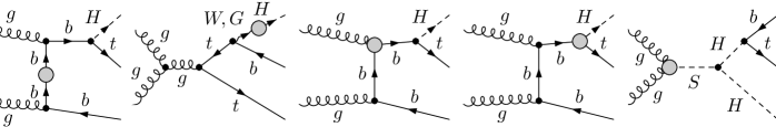
Figure 3: Representative one-loop self-energy and vertex diagrams. The shaded regions are the one-particle irreducible two- and three-point vertices including the counterterms. $G$ denotes the $W$ Goldstone bosons.

Figure 4: Representative diagrams with irreducible four- and five-point vertices. $S$ denotes a Higgs or Goldstone boson, $V$ an electroweak gauge boson, $\tilde{q}$ a squark, and $\tilde{\chi}$ a chargino or neutralino.

Figure 5: Representative diagrams for real photon emission.

In this section we discuss the NLO EW contributions to the $gg\to H^{-}t\bar{b}$ subprocess. These corrections are of order ${\cal O}(\alpha_{s}^{2}\alpha^{2})$. Other corrections of the same order arising from the remaining subprocesses in Eq. (3), Eq. (4) and Eq. (5) are much smaller and will be neglected.

The NLO EW contributions are composed of a virtual part and a real part. The virtual part comprises the contributions of bottom-quark and top-quark self-energies, of triangle, box and pentagon diagrams, and of wave-function corrections. For illustration, some generic classes of self-energy and vertex diagrams including the corresponding counterterms are shown in Fig. 3. The box and pentagon diagrams are UV finite, a representative sample is depicted in Fig. 4.

The virtual part contains UV divergences, soft, and collinear singularities. The UV divergences are canceled by renormalization, which requires the choice of a renormalization scheme. We use the same renormalization procedure as the one described in [16] for the process $\bar{b}b\rightarrow W^{\mp}H^{\pm}$. This is a hybrid of on-shell and $\overline{\text{DR}}$ schemes originally defined in [19]. We summarize here the main points and refer to [16] for more details. The calculation is done by using the technique of constrained differential renormalization [20] which is, at one-loop level, equivalent to regularization by dimensional reduction [21, 22]. The on-shell scheme is used for the fermion sector, the fine-structure constant, and the charged Higgs-boson mass. The charged Higgs field and $\tan\beta$ are renormalized in the $\overline{\text{DR}}$ scheme. Hence, the correct on-shell behavior of the external $H^{-}$ must be ensured by including the finite wave-function renormalization factor [23]

$$\sqrt{Z_{H^{-}H^{+}}}=1-\frac{1}{2}\operatorname{Re}\frac{\partial}{\partial p^{2}}\hat{\Sigma}_{H^{-}H^{+}}(p^{2})\big{|}_{p^{2}=M_{H^{\pm}}^{2}},$$ (11)

where $\hat{\Sigma}_{H^{-}H^{+}}(p^{2})$ is the $H^{\pm}$ renormalized self-energy, and the mixing of $H^{-}$ with $W$ and charged Goldstone bosons (see Fig. 3).

To make the EW corrections independent of $\ln m_{f}$ from the light fermions $f\neq t$, we use the fine-structure constant at $M_{Z}$, $\alpha=\alpha(M_{Z})$ as an input parameter. This means that we have to modify the counterterm according to

$$\delta Z_{e}^{\alpha(M_{Z})} = \delta Z_{e}^{\alpha(0)}-\frac{1}{2}\Delta\alpha(M_{Z}^{2}),$$

$$\Delta\alpha(M_{Z}^{2}) = \frac{\partial\Sigma_{T}^{AA}}{\partial k^{2}}\bigg{|}_{k^{2}=0}-\frac{\operatorname{Re}\Sigma_{T}^{AA}(M_{Z}^{2})}{M_{Z}^{2}},$$ (12)

with the photon self-energy from the light fermions only to avoid double counting. In the calculation of EW corrections, the couplings in Eq. (6) are used.

Concerning the bottom quark, the pole mass enters the kinematical variables of the matrix element and the phase space, whereas the $b$ Yukawa couplings are usually improved by using the running $m_{b}$ (as done e.g. in the calculation of NLO QCD contributions [1]). For NLO EW calculations, however, such a distinction is not possible since the $b$-quark mass is of EW origin. One has to use a common value for the kinematical variables and for the Yukawa couplings in order to obtain UV finiteness because of the interplay between the bottom-mass, the bottom-Goldstone and the bottom-Higgs couplings in the renormalization of the EW contributions. The use of different masses would violate important Ward identities involving $m_{b}$ (see e.g. [24]), leading to an incomplete cancellation of UV poles. Hence, one can either choose the pole mass or the running mass in all places. We have decided to take the running mass $m_{b}=m_{b}^{\overline{\text{DR}}}(\mu_{R})$ because a more accurate treatment of the Yukawa couplings is more significant than an accurate treatment of the kinematics. For infrared-safe observables the kinematical logarithms of $m_{b}$ cancel. For non-infrared-safe observables like in our case (see discussion below) some contribution of $\alpha\log(m_{b})$ remains. Ideally, this would be $\alpha\log(m_{b}^{\text{pole}})$. The difference $\alpha\log(m_{b}^{\overline{DR}}/m_{b}^{\text{pole}})$ is, however, of higher order and numerically very small, and hence can be neglected in our study. Moreover, if the hadronization of the $b$ quark is taken into account, the kinematical $m_{b}$ dependence is expected to be irrelevant and one can regard the kinematical $m_{b}$ as a regulator.

We classify the virtual part into two gauge-invariant groups. The first group consists of one-loop diagrams contributing to the process

$$g+g\to H^{-}+H^{+*}\to H^{-}+t+\bar{b},$$ (13)

where the virtual $H^{+*}$ can be on-shell, see Fig. 3 and Fig. 4 (box diagrams). The second group is the remainder, which is free of resonating propagators. The first group is UV and infrared finite since the channel $g+g\to H^{-}+H^{+*}$ does not occur at tree level. Because the intermediate $H^{+*}$ can be on-shell, special care has to be taken for the numerical integration over the phase space. The resonance propagator reads (zero-width approximation)

$$\Delta_{H^{\pm}}=\frac{1}{q^{2}-M_{H^{\pm}}^{2}+i\epsilon}=\text{PV}\left(\frac{1}{q^{2}-M_{H^{\pm}}^{2}}\right)-i\pi\delta(q^{2}-M_{H^{\pm}}^{2}),$$ (14)

where PV denotes the Cauchy principal value. The principal-value part can be calculated by imposing a small cut on $q^{2}$ around the pole. The contribution from the $\delta$ function part is nonvanishing because the imaginary part of the on-shell propagator can multiply by the imaginary part of the loop integrals, hence the corresponding one-loop amplitude can interfere with the tree-level amplitude. We have checked that this contribution is indeed nonzero, but small. A naive calculation taking into account only the principal value part would lead to an incorrect result. For practical purposes, a better method is introducing a small width in the resonance propagator,

$$\Delta_{H^{\pm}} = \frac{1}{q^{2}-M_{H^{\pm}}^{2}+iM_{H^{\pm}}\Gamma_{H^{\pm}}}.$$ (15)

We have checked that the result is practically independent of the small values of the width and agrees with the sum of the principal value and $\delta$ function contributions. We also notice that this method gives smaller integration error. As will be shown in the numerical study, the effect of the $H^{-}H^{+*}$ production mechanism is small at the cross section level, but is of importance for differential cross sections.

The real EW corrections arise from the photonic bremsstrahlung process,

$$g+g\to H^{-}+t+\bar{b}+\gamma,$$ (16)

with the corresponding Feynman diagrams shown in Fig. 5. This contribution is divergent in the soft limit ($p_{\gamma}^{0}\to 0$) and contains quasi-collinear corrections [25] proportional to $\alpha\log(m_{b}^{2}/E_{b}^{2})$, $E_{b}$ being the $b$-quark energy, in the limit $p_{b}p_{\gamma}\to{\cal O}(m_{b}^{2})$. The $b$-quark mass is used for regularization and to separate the singular terms. A fictitious photon mass ($\lambda_{\gamma}$) is used for regularization of the soft singularities. If we consider the total cross section, i.e.  without applying the cuts in Eq. (1), the soft and quasi-collinear singularities cancel completely in the sum of the virtual and the real contributions, according to the Kinoshita-Lee-Nauenberg theorem [26, 27]. This requires that we have to use $m_{b}=m_{b}^{\overline{\text{DR}}}(\mu_{R})$ as in the virtual amplitudes. If the cuts in Eq. (1) are imposed then the soft singularities still cancel, but the quasi-collinear singularities do not, since the cuts requiring bottom-photon separation are not collinear safe. In this case, some quasi-collinear singularities remain and are regularized by the bottom mass. Those left-over singularities can be separated, as discussed below. If a sufficiently collinear $b$-photon system is recombined before applying cuts then the quasi-collinear singularities cancel, but the result will depend on the recombination parameter. As done in the previous study for the NLO QCD corrections [1], we assume in this paper bottom-photon separation, and hence no photon recombination is applied.

The dipole subtraction method [28, 29, 25, 30] is used to extract the singularities from the real corrections and combine them with the virtual contribution. The subtraction method for doing the phase-space integration for the radiation process Eq. (16) arranges the integral in the following way,

$$\sigma_{\text{real}}=\int_{4}\left[\,d\sigma_{\text{real}}\;\theta(p_{b})-d\sigma_{\text{sub}}\;\theta(\tilde{p}_{b})\,\right]+\int_{4}d\sigma_{\text{sub}}\;\theta(\tilde{p}_{b}).$$ (17)

The subscript $4$ refers to the 4-body final state including the radiated photon, $\theta$ is a function to impose the kinematical cuts defined in Eq. (1), $\tilde{p}_{b}$ is a function of $p_{i}$ with $i=$ $H^{-}$, $t$, $b$, $\gamma$, with the definition given in [29, 25, 30]. The subtraction function $d\sigma_{\text{sub}}\theta(\tilde{p}_{b})$ has to be chosen such that the first integral is finite and the second one can be partially analytically integrated over the singular variables. The function $d\sigma_{\text{sub}}$ has the same singular structure as $d\sigma_{\text{real}}$ pointwise in the phase space. There are two ways to deal with the cut function.
i) We require that (the pseudorapidity cut is neglected to simplify the discussion)

$$\theta(\tilde{p}_{b})\to\theta(p_{b})\quad\text{or}\quad\tilde{p}_{b}\to p_{b}$$ (18)

in the singular limits (the soft limit is trivially satisfied), which implies that $\theta(\tilde{p}_{b})$ is not collinear safe, so that the first integral is soft and (quasi-)collinear finite. All soft and quasi-collinear singularities are contained in the second integral. All soft and some quasi-collinear singularities are canceled in the sum with the virtual contribution. The leftover quasi-collinear singularities, regularized by $m_{b}$, can be factorized and separated. A detailed procedure including the definition of $\tilde{p}_{b}$ is described in [30]. A consequence of the condition (18) is that, in the calculation of the first integral, we can set $m_{b}=0$ in the kinematics (but not in the Yukawa couplings).
ii) We require that the cut function $\theta(\tilde{p}_{b})$ is infrared safe as in [29, 25] so that the sum of the second integral and the virtual contribution is independent of soft and quasi-collinear singularities. Specifically, it means that the condition (18) is satisfied for the soft limit but not for the collinear limit. The first integral, therefore, contains the leftover quasi-collinear singularities. Since the result is finite one can do it numerically. In this approach, one has to keep $m_{b}$ everywhere. We have implemented both approaches and found good agreement for the cross section and the distributions. Moreover, the result of the dipole subtraction method is compared with the one of the phase-space slicing method, as illustrated in Fig. 6. In the numerical analysis, we will present the results of the dipole subtraction method because the integration errors are smaller.

The above treatment of the kinematical cuts in the dipole subtraction method is also applied for the bottom-quark histograms displayed in Section 4.4.

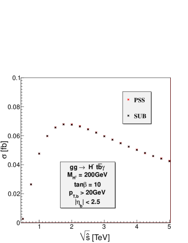
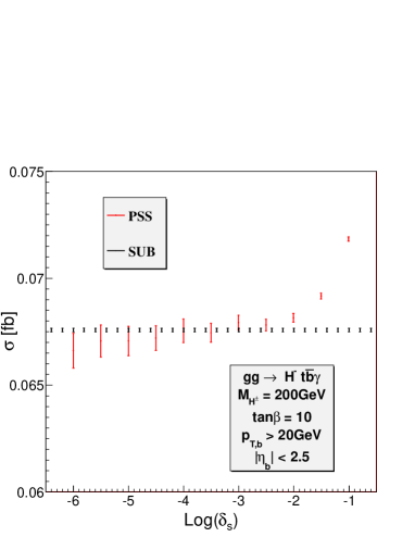
Figure 6: Partonic cross sections as functions of the center-of-mass energy $\sqrt{\hat{s}}$ in the left panel and of the cutoff parameter $\delta_{s}$ in the right panel are presented for the $gg\to H^{-}t\bar{b}\gamma$ process. The results are obtained by using the phase space slicing method (PSS) and the dipole subtraction method (SUB, straight line) in the CPX scenario. The photon mass regulator $\ln\lambda_{\gamma}$ is set to zero.

Finally, the hadronic cross section at NLO is written in the following way as the sum of the improved Born approximation and the genuine loop and radiation terms for the $gg$ subprocess,

$$\sigma^{pp}_{\text{NLO}} = \sigma^{pp}_{\text{IBA}}+\Delta^{pp/gg}_{\text{EW}}\,,$$ (19)

with

$$\Delta^{pp/gg}_{\text{EW}} = \int{\textrm{d}}x_{1}{\textrm{d}}x_{2}\;F_{g}^{p}(x_{1},\mu_{F})F_{g}^{p}(x_{2},\mu_{F})\;\Delta^{gg}_{\text{EW}}(\alpha_{s}^{2}\alpha^{2},\mu_{R})\,.$$ (20)

Thereby, $\Delta_{\text{EW}}^{gg}$ is the sum of the virtual and the real corrections at the partonic level, as discussed above. The IBA part of the cross section results from the various sources at the partonic level,

$$\sigma^{pp}_{\text{IBA}} = \sigma^{pp/gg}_{\text{IBA}}+\sigma^{pp/q\bar{q}}_{\text{IBA}}+\sigma^{pp/b\bar{b}}_{\text{IBA}}+\sigma^{pp/g\gamma}_{\text{IBA}}\,,$$ (21)

as discussed in Section 2.

4 Numerical studies

4.1 Input parameters

We use the same set of input parameters as in [16] for the sake of comparison. For the SM sector:

$$\alpha_{s}(M_{Z}) =0.1197,\hskip 8.53581pt \alpha(M_{Z}) =1/128.926,$$ (22)

$$M_{W} =80.398~{}\text{GeV},\hskip 8.53581pt M_{Z} =91.1876~{}\text{GeV},$$

$$m_{t} =173.1~{}\text{GeV},\hskip 8.53581pt \overline{m}_{b}(\overline{m}_{b}) =4.2~{}\text{GeV}.$$

We take here $\alpha_{s}=\alpha_{s}^{\overline{\text{MS}}}(\mu_{R})$ at three-loop order [31]. $\overline{m}_{b}(\overline{m}_{b})$ is the QCD-$\overline{\text{MS}}$ $b$-quark mass, while the top-quark mass is understood as the pole mass. The CKM matrix is approximated to be unity.

For the soft SUSY-breaking parameters, the adapted CP-violating benchmark scenario (CPX) [32, 33] is used,

$$\begin{aligned} |\mu|&=2~{}\text{TeV},|M_{2}|=200~{}\text{GeV},\,|M_{3}|=1~{}\text{TeV},\,|A_{t}|=|A_{b}|=|A_{\tau}|=900~{}\text{GeV},\\ M_{\tilde{Q}}&=M_{\tilde{D}}=M_{\tilde{U}}=M_{\tilde{L}}=M_{\tilde{E}}=M_{\text{SUSY}}=500~{}\text{GeV},\,|M_{1}|=5/3\tan^{2}\theta_{W}|M_{2}|.\end{aligned}$$ (23)

We set $A_{f}=0$ for $f=e,\mu,u,d,c,s$ since the Yukawa couplings of the first two fermion generations proportional to the small fermion masses are neglected in our calculations. With the convention that $M_{2}$ is real, the complex phases of the trilinear couplings $A_{t}$, $A_{b}$, $A_{\tau}$ and the gaugino-mass parameters $M_{1}$ and $M_{3}$ are chosen as default according to

$$\phi_{t}=\phi_{b}=\phi_{\tau}=\phi_{1}=\phi_{3}=\frac{\pi}{2},$$ (24)

unless specified otherwise. The phase of $\mu$ is chosen to be zero. This is consistent with the experimental data of the electric dipole moment and the explanation of the muon anomalous magnetic moment discrepancy between the present data and the standard model prediction (see e.g. [34]). We will study the dependence of our results on $\tan\beta$, $M_{H^{\pm}}$ and $\phi_{t}$ in the numerical analysis.

The scale of $\alpha_{s}$ in the SUSY-QCD resummation of the effective bottom-Higgs couplings in Eq. (9) of [16] is set to be $Q=(m_{\tilde{b}_{1}}+m_{\tilde{b}_{2}}+m_{\tilde{g}})/3$. This choice is justified by the two-loop results for the $\Delta_{b}$ corrections [35, 36, 37]. If not otherwise specified, we set the renormalization scale equal to the factorization scale, $\mu_{R}=\mu_{F}$, in all numerical results. Our default choice for the factorization scale is $\mu_{F0}=(m_{t}+M_{H^{\pm}})/3$, which is justified by the NLO QCD results [1]. We use the MRST2004qed code to calculate the PDFs.

Our study is done for the LHC at $7~{}\text{TeV}$, $8~{}\text{TeV}$ and $14~{}\text{TeV}$ center-of-mass energy ($\sqrt{s}$). In the following we show the dependence of the cross section on $\tan\beta$, $M_{H^{\pm}}$ and $\phi_{t}$, and various differential distributions for the default parameter point. Since the results of the different center-of-mass energies look quite similar in shape and differ mainly by the magnitude of the cross section, our discussion essentially applies to all displayed cases of the total energy.

4.2 Calculations and checks

The results in this paper have been obtained by two independent calculations. We have produced, with the help of FeynArts-3.4[38, 39] and FormCalc-6.0[22], two different Fortran 77 codes. The loop integrals contain five-point tensor integrals up to rank three, and four-point tensor integrals up to rank three. The pentagon integrals are reduced to the box integrals by using the reduction methods in [40, 41, 42]. The two-, three- and four-point tensor integrals are further reduced to the scalar integrals by using the Passarino-Veltman reduction method [43]. The loop integrals are evaluated with two independent libraries, LoopTools/FF[44, 45, 46] using the five-point reduction method of [40] and our in-house library LoopInts using the five-point reduction method of [42]. The latter uses the method of [47, 48, 49], treats all the internal masses as complex parameters and has an option to use quadruple precision, on the fly, when numerical instabilities are detected. The phase-space integration is done by using the Monte Carlo integrators BASES [50] and VEGAS [51]. The results of the two codes are in good agreement. On top, we have also performed a number of other checks:

For the process $gg\to H^{-}t\bar{b}$, we have verified that the results are QCD gauge invariant at LO, IBA and NLO. This nontrivial check, which can detect a bug in the Feynman rules and in the tensor reduction procedure, can be easily done in practice by changing the numerical value of the gluon polarization vector $\epsilon_{\mu}(p,q)$, where $p$ is the gluon momentum and $q$ is an arbitrary reference vector. QCD gauge invariance means that the squared amplitudes are independent of $q$. More details can be found in [52]. The common checks of UV and infrared finiteness are done for the NLO calculations.

4.3 LO, IBA and NLO cross sections

The LO, IBA and NLO cross sections as functions of $\tan\beta$, the phase $\phi_{t}$, and $M_{H^{\pm}}$ are shown at $14~{}\text{TeV}$ and $8~{}\text{TeV}$ on the left and right columns of Fig. 7, respectively, and at $7~{}\text{TeV}$ on the left column of Fig. 8. The relative corrections $\delta$, with respect to the LO cross section, are defined as $\delta=(\sigma_{\text{IBA/NLO}}-\sigma_{\text{LO}})/\sigma_{\text{LO}}$.

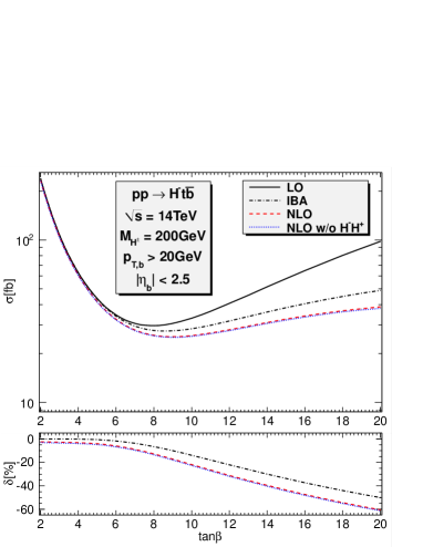
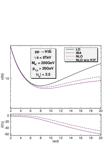
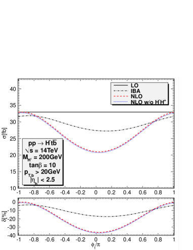
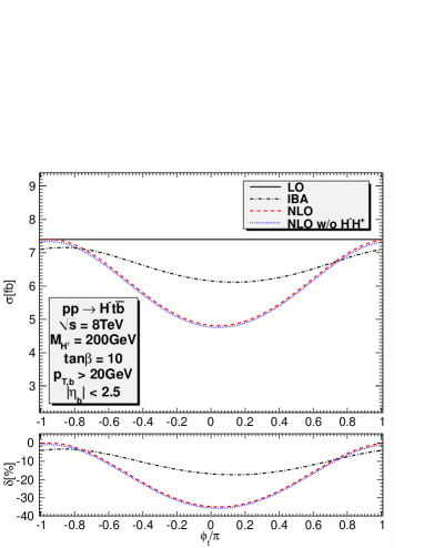
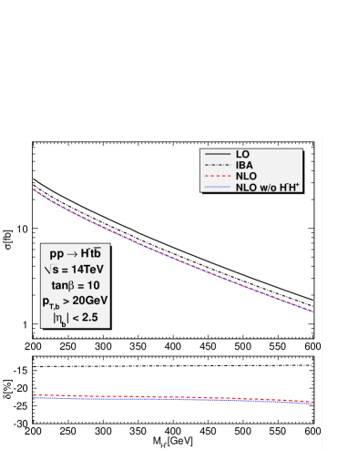
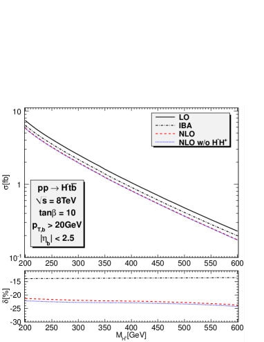
Figure 7: The cross section for $pp\to H^{-}t\bar{b}$ as function of $\tan\beta$, $\phi_{t}$, ${M_{H^{\pm}}}$ in various steps of approximation LO, IBA, and NLO, for $\sqrt{s}=14~{}\text{TeV}$ (left) and $\sqrt{s}=8~{}\text{TeV}$ (right). The lower part of each panel shows the relative corrections to the LO results. Also shown is the NLO result without the $H^{-}H^{+*}$ production mechanism.

We first study the effects of $\Delta_{b}$ resummation in the effective bottom-Higgs couplings. For small values of $\tan\beta$ the left-chirality contribution proportional to $m_{t}/\tan\beta$ is dominant while the right-chirality contribution proportional to $m_{b}\tan\beta$ dominates at large $\tan\beta$. The cross section has a minimum around $\tan\beta=8$. The effect of $\Delta_{b}$ resummation is best understood by comparing the phase-dependence plot and the others. The important point is that $\Delta_{b}$ is a complex number and only its real part can interfere with the LO amplitude. Thus, the $\Delta_{b}$ effect is minimum at $\phi_{t}=\pm\pi/2$ where the dominant contributions are purely imaginary and is largest at $\phi_{t}=0,\pm\pi$. The phase-dependence plot shows that the $\Delta m_{b}^{\text{SEW}}$ effect can be more than $10\%$. From the $\tan\beta$ dependence plots where $\Delta_{b}$ is mostly imaginary we see the effect of order ${\cal O}(\Delta_{b}^{2})$, which is about $-15\%$ at $\tan\beta=10$.

We now turn to the NLO cross sections, which include the complete EW corrections to the process $gg\to H^{-}t\bar{b}$. Fig. 7 also contains the effect of the $H^{-}H^{+*}$ resonance mechanism, which is almost invisible at the cross section level. The NLO cross section depends strongly on $\phi_{t}$. The IBA results are always closer to the NLO values rather than to the LO ones. In particular, for the phase dependence, the IBA shows the qualitative features of the NLO prediction while the LO cross section is a constant. After subtracting the $\Delta m_{b}^{\text{SEW}}$ corrections, the remaining NLO EW contributions are still sizeable. The relative correction increases with $\tan\beta$ and ${M_{H^{\pm}}}$ for the default value $\phi_{t}=\pi/2$; for fixed default values of $\tan\beta$ and ${M_{H^{\pm}}}$, it is maximal (about $40\%$) at $\phi_{t}=0$. As an aside, we remark that the IBA and NLO EW effects for the process $gg\to H^{-}t\bar{b}$ are similar to the ones found in the $b\bar{b}\to W^{-}H^{+}$ study [16]. The hierarchy of the LO, IBA and NLO contributions is also the same as the one found in [12].

Table 1: The total cross section in fb for $pp\to H^{-}t\bar{b}$ including the IBA of the four subprocesses and EW NLO corrections to $gg\to H^{-}t\bar{b}$ at $\sqrt{s}=14~{}\text{TeV}$. The charged Higgs-boson masses are given in GeV. The numbers in brackets show the integration uncertainty in the last digit when they are significant.

$\tan\beta$	$M_{H^{\pm}}$	$\sigma_{\text{IBA}}^{pp/gg}$		$\sigma_{\text{IBA}}^{pp/q\bar{q}}$		$\sigma_{\text{IBA}}^{pp/b\bar{b}}$		$\sigma_{\text{IBA}}^{pp/g\gamma}$		$\Delta_{\text{EW}}^{pp/gg}$		all
5	200	38.	833(7)	3.	581	0.	319	0.	559	-1.	522(5)	41.	770(8)
10	200	25.	447(5)	2.	372	0.	210	0.	367	-2.	642(4)	25.	754(6)
20	200	43.	992(8)	3.	973	0.	357	0.	630	-10.	24(1)	38.	71(1)
10	300	10.	740(2)	0.	457	0.	075	0.	139	-1.	126(2)	10.	285(3)
10	400	5.	207(1)	0.	143	0.	031	0.	064	-0.	556(1)	4.	889(2)
10	600	1.	4829(3)	0.	0244	0.	0069	0.	0183	-0.	1842(3)	1.	3483(5)

Table 2: Similar to Table 1 but for $\sqrt{s}=8~{}\text{TeV}$.

$\tan\beta$	$M_{H^{\pm}}$	$\sigma_{\text{IBA}}^{pp/gg}$		$\sigma_{\text{IBA}}^{pp/q\bar{q}}$		$\sigma_{\text{IBA}}^{pp/b\bar{b}}$		$\sigma_{\text{IBA}}^{pp/g\gamma}$		$\Delta_{\text{EW}}^{pp/gg}$		all
5	200	8.	197(2)	1.	314	0.	051	0.	151	-0.	315(1)	9.	399(2)
10	200	5.	369(1)	0.	871	0.	034	0.	099	-0.	548(2)	5.	826(2)
20	200	9.	295(2)	1.	456	0.	058	0.	171	-2.	115(7)	8.	864(8)
10	300	1.	9970(6)	0.	1377	0.	0101	0.	0332	-0.	2056(8)	1.	9724(10)
10	400	0.	8535(2)	0.	0361	0.	0035	0.	0137	-0.	0900(3)	0.	8169(4)
10	600	0.	18947(5)	0.	00444	0.	00056	0.	00315	-0.	02328(8)	0.	17435(10)

Table 3: Similar to Table 1 but for $\sqrt{s}=7~{}\text{TeV}$.

$\tan\beta$	$M_{H^{\pm}}$	$\sigma_{\text{IBA}}^{pp/gg}$		$\sigma_{\text{IBA}}^{pp/q\bar{q}}$		$\sigma_{\text{IBA}}^{pp/b\bar{b}}$		$\sigma_{\text{IBA}}^{pp/g\gamma}$		$\Delta_{\text{EW}}^{pp/gg}$		all
5	200	5.	3652(9)	0.	9885	0.	0311	0.	1058	-0.	2049(6)	6.	286(1)
10	200	3.	5138(6)	0.	6551	0.	0205	0.	0695	-0.	3552(5)	3.	9037(8)
20	200	6.	085(1)	1.	095	0.	035	0.	119	-1.	367(2)	5.	967(2)
10	300	1.	2570(2)	0.	0974	0.	0058	0.	0224	-0.	1292(2)	1.	2534(3)
10	400	0.	5164(1)	0.	0242	0.	0019	0.	0089	-0.	0544(1)	0.	4971(1)
10	600	0.	10583(2)	0.	00268	0.	00027	0.	00191	-0.	01295(2)	0.	09774(3)

Table 1 shows separately the IBA results for the various subprocesses together with the NLO EW corrections to $gg\to H^{-}t\bar{b}$ at $\sqrt{s}=14~{}\text{TeV}$ for different values of ${M_{H^{\pm}}}$ and $\tan\beta$. Similar results are presented in Table 2 and Table 3, but now for $\sqrt{s}=8~{}\text{TeV}$ and $\sqrt{s}=7~{}\text{TeV}$, respectively. We observe that the $gg$ contributions are dominant; they contribute more than $90\%$ ($83\%$) of the total IBA for $\sqrt{s}=14~{}\text{TeV}$ ($\sqrt{s}=7~{}\text{TeV}$). The contribution of the $b\bar{b}$ channel is below $1\%$; the $g\gamma$ channel contribution is slightly larger. The NLO EW contributions are comparable in size to the $q\bar{q}$ contributions, but with the opposite sign.

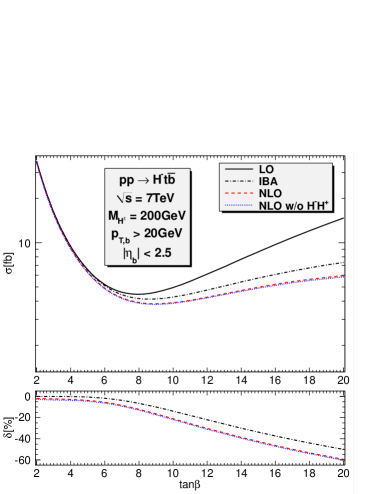
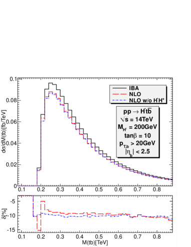
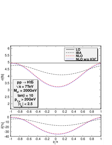
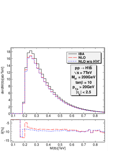
Figure 8: Left column: the LO, IBA and NLO cross section for $pp\to H^{-}t\bar{b}$ as function of $\tan\beta$, $\phi_{t}$, and ${M_{H^{\pm}}}$, for $\sqrt{s}=7~{}\text{TeV}$. Right column: the IBA and NLO EW invariant mass distributions of the $t\bar{b}$ system for $pp\to H^{-}t\bar{b}$ at $14$, $8$ and $7~{}\text{TeV}$. The lower panels show the relative corrections. Also shown is the NLO result without the $H^{-}H^{+*}$ production mechanism.

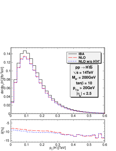
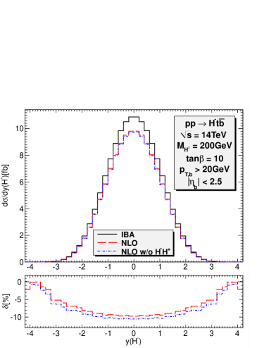
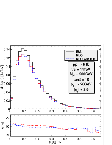
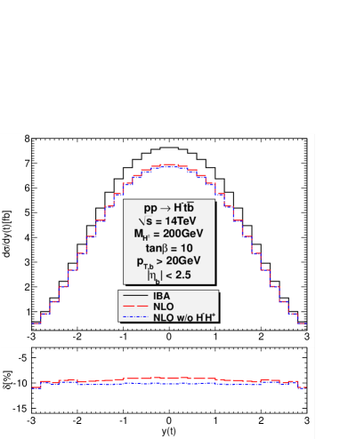
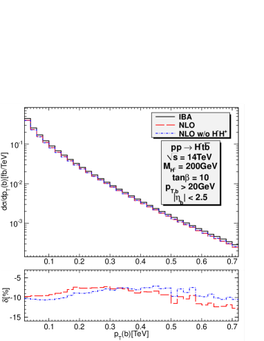
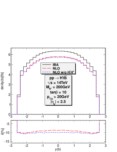
Figure 9: The IBA and NLO distributions of transverse momentum (left) and rapidity (right) for $H^{-}$, $t$, $\bar{b}$ at $14~{}\text{TeV}$. The lower panels show the relative corrections. Also shown is the NLO result without the $H^{-}H^{+*}$ production mechanism.

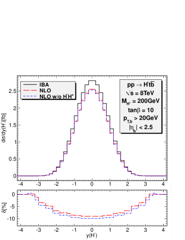
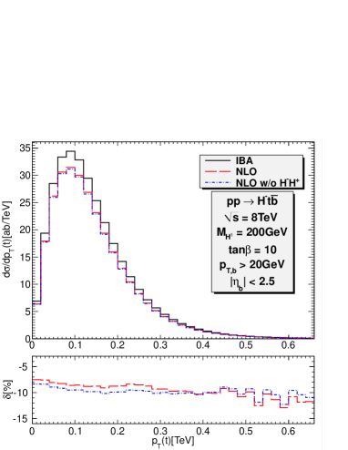
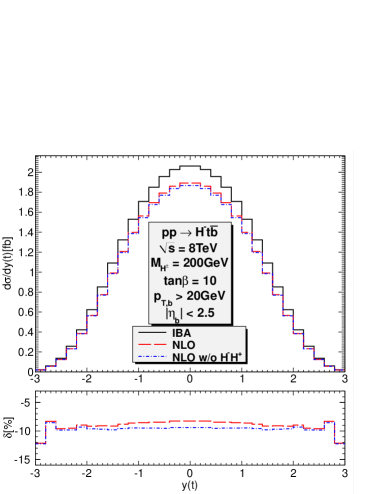
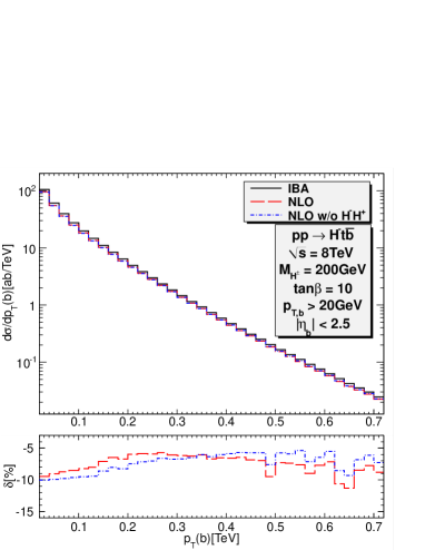
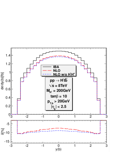
Figure 10: Similar to Fig. 9 but for $\sqrt{s}=8~{}\text{TeV}$.

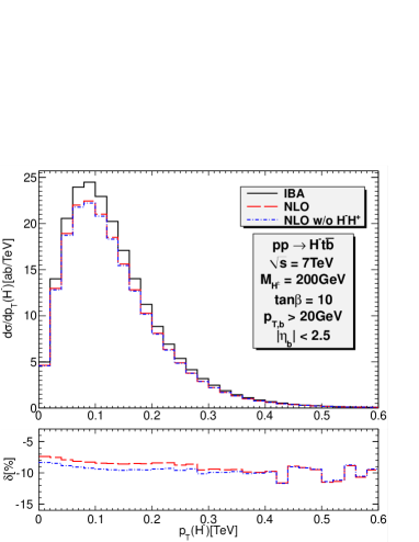
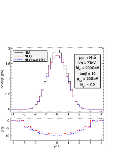
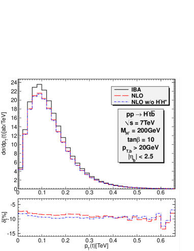
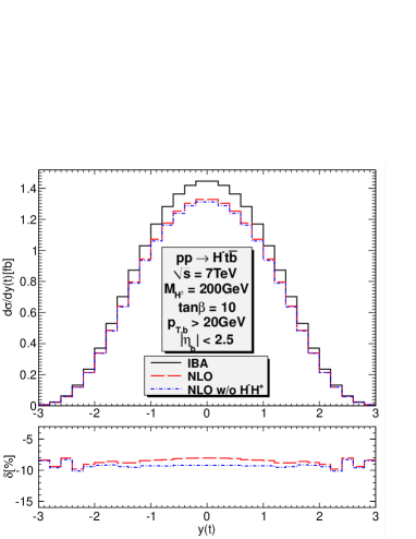
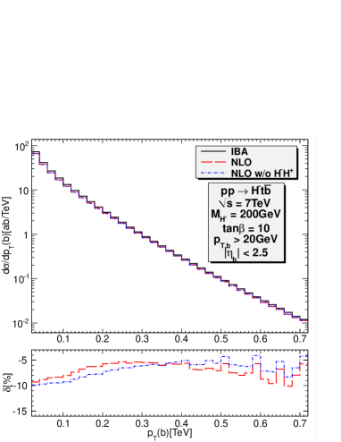
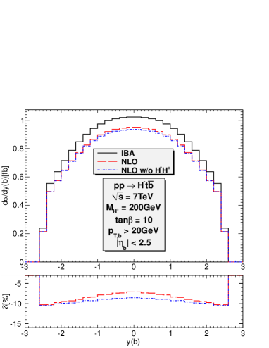
Figure 11: Similar to Fig. 9 but for $\sqrt{s}=7~{}\text{TeV}$.

4.4 Differential distributions

We now consider the differential distributions of various kinematical variables, in the IBA and including the NLO EW corrections. The relative correction is defined with respect to the IBA differential cross section, $\delta=(d\sigma_{\text{NLO}}-d\sigma_{\text{IBA}})/d\sigma_{\text{IBA}}$. All results are shown in the right column of Fig. 8 and in Figs. 9, 10 and 11.

The effect of the $H^{-}H^{+*}$ production mechanism is best seen in the right column of Fig. 8. The $t\bar{b}$ invariant mass distribution shows the singular pole structure at $M_{t\bar{b}}=M_{H^{\pm}}=200~{}\text{GeV}$ if this channel is included. This effect is also visible in other distributions.

Distributions for the individual particles separately are shown in Fig. 9. for $\sqrt{s}=14~{}\text{TeV}$, and in Figs. 10 and 11 for the lower energies 8 and 7 TeV. The results are very similar and differ essentially in the absolute size of the cross section at the different energies.

For the charged Higgs boson, the relative correction is negative, decreases with $p_{T}(H^{-})$ and has a minimum (about $-10\%$) at the central rapidity.

For the top quark, the behavior of the $p_{T}$ distribution is similar to the one of the charged Higgs boson. The EW corrections are negative and decrease with $p_{T}$, consistent with Sudakov corrections $\alpha\log^{n}(p_{T}^{2}/M_{W}^{2})$ with $n=1,2$. For the rapidity distribution, the relative correction is rather flat (about $-10\%$) in the region $|y_{t}|<3$.

The distributions of the bottom quark are quite different from the ones of the heavy particles. At tree level (see the IBA curve), the cross section is larger at low $p_{T}$ due to collinear bottom-quark radiation off gluons. The relative correction increases and reaches the maximal value at $p_{T}\approx 0.3~{}\text{TeV}$ and then follows the trend of decreasing with $p_{T}$ as for the other particles. This behavior can be explained by the interplay between the leading weak Sudakov correction $\alpha\log^{2}(p_{T}^{2}/M_{W}^{2})$ and the QED quasi-collinear correction $\alpha\log(m_{b}^{2}/p_{T}^{2})$ from photon radiation off the bottom quark. The latter is more important at low $p_{T}$ while the former dominates in the high energy regime. For the rapidity distribution, the correction is smallest in the central region.

5 Conclusions

In this paper we have studied the production of charged Higgs bosons in association with a top quark and a tagged bottom quark at the LHC in the context of the complex MSSM. Cuts on the transverse momentum and rapidity of the bottom quark are applied. At tree level, the $gg$ fusion is dominant among various subprocesses with quarks or photon in the initial state; for this parton process, the NLO EW corrections have been calculated and discussed.

Since the tree-level amplitudes are proportional to the top-bottom-Higgs coupling, we have examined the effective-coupling approximation and compared it to the full NLO result. The dependence of the cross section on $\tan\beta$, $M_{H^{\pm}}$ and the phase $\phi_{t}$ of the trilinear coupling $A_{t}$ has also been studied.

Numerical results have been presented for the CPX scenario. The production cross section shows a strong dependence on $\tan\beta$, $M_{H^{\pm}}$ and $\phi_{t}$. Large production rates occur for small $\tan\beta$, small $M_{H^{\pm}}$ and phases $\phi_{t}$ around $\pm\pi$. At LO, the cross section increases strongly with large $\tan\beta$. This behavior is, however, significantly reduced when NLO corrections are included. An interesting feature is the $\phi_{t}$ dependence: while the LO cross section is just a constant, the IBA and NLO results show a strong dependence with a minimum at $\phi_{t}=0$.

We have also presented various differential distributions of the final state particles, where the NLO EW corrections are usually negative.

Acknowledgments
D.T.N. and L.D.N. would like to thank the Max-Planck Insitut für Physik in Munich where most of this work has been done and acknowledge the support from the Deutsche Forschungsgemeinschaft via the Sonderforschungsbereich/Transregio SFB/TR-9 Computational Particle Physics. L.D.N. is partially supported by the Vietnam Academy of Science and Technology between the Vietnam-France collaboration program in particle physics under the grant VAST.HTQT.PHAP.04/2012-2013.

References

- [1] S. Dittmaier, M. Kramer, M. Spira, and M. Walser, Phys.Rev. D83, 055005 (2011), arXiv:0906.2648.
- [2] D. Miller, S. Moretti, D. Roy, and W. J. Stirling, Phys.Rev. D61, 055011 (2000), hep-ph/9906230.
- [3] D. Roy, AIP Conf.Proc. 805, 110 (2006), hep-ph/0510070.
- [4] S.-h. Zhu, Phys.Rev. D67, 075006 (2003), hep-ph/0112109.
- [5] G.-p. Gao, G.-r. Lu, Z.-h. Xiong, and J. M. Yang, Phys.Rev. D66, 015007 (2002), hep-ph/0202016.
- [6] T. Plehn, Phys.Rev. D67, 014018 (2003), hep-ph/0206121.
- [7] E. L. Berger, T. Han, J. Jiang, and T. Plehn, Phys.Rev. D71, 115012 (2005), hep-ph/0312286.
- [8] M. Beccaria, G. Macorini, L. Panizzi, F. Renard, and C. Verzegnassi, Phys.Rev. D80, 053011 (2009), arXiv:0908.1332.
- [9] N. Kidonakis, PoS HEP2005, 336 (2006), hep-ph/0511235.
- [10] N. Kidonakis, Phys.Rev. D82, 054018 (2010), arXiv:1005.4451.
- [11] W. Peng et al., Phys. Rev. D73, 015012 (2006), hep-ph/0601069, [Erratum-ibid.D80:059901,2009].
- [12] B. Kniehl, M. Maniatis, and M. Weber, Phys.Rev. D83, 015011 (2011), 1009.3929.
- [13] J. L. Diaz-Cruz and O. A. Sampayo, Phys. Rev. D50, 6820 (1994).
- [14] F. Borzumati, J. L. Kneur, and N. Polonsky, Phys. Rev. D60, 115011 (1999), hep-ph/9905443.
- [15] A. D. Martin, R. G. Roberts, W. J. Stirling, and R. S. Thorne, Eur. Phys. J. C39, 155 (2005), hep-ph/0411040.
- [16] T. N. Dao, W. Hollik, and D. N. Le, Phys. Rev. D83, 075003 (2011), arXiv:1011.4820.
- [17] M. S. Carena, D. Garcia, U. Nierste, and C. E. M. Wagner, Nucl. Phys. B577, 88 (2000), hep-ph/9912516.
- [18] T. N. Dao, Ph.D. thesis, Technische Universität München, 2012 .
- [19] M. Frank et al., JHEP 02, 047 (2007), hep-ph/0611326.
- [20] F. del Aguila, A. Culatti, R. Munoz Tapia, and M. Perez-Victoria, Nucl. Phys. B537, 561 (1999), hep-ph/9806451.
- [21] W. Siegel, Phys. Lett. B84, 193 (1979).
- [22] T. Hahn and M. Perez-Victoria, Comput. Phys. Commun. 118, 153 (1999), hep-ph/9807565.
- [23] W. Hollik and D. Nhung, JHEP 1101, 060 (2011), 1008.2659.
- [24] N. Baro, F. Boudjema, and A. Semenov, Phys.Rev. D78, 115003 (2008), 0807.4668.
- [25] S. Catani, S. Dittmaier, M. H. Seymour, and Z. Trocsanyi, Nucl. Phys. B627, 189 (2002), hep-ph/0201036.
- [26] T. Kinoshita, J. Math. Phys. 3, 650 (1962).
- [27] T. D. Lee and M. Nauenberg, Phys. Rev. 133, B1549 (1964).
- [28] S. Catani and M. H. Seymour, Nucl. Phys. B485, 291 (1997), hep-ph/9605323.
- [29] S. Dittmaier, Nucl. Phys. B565, 69 (2000), hep-ph/9904440.
- [30] S. Dittmaier, A. Kabelschacht, and T. Kasprzik, Nucl.Phys. B800, 146 (2008), arXiv:0802.1405.
- [31] Particle Data Group, C. Amsler et al., Phys. Lett. B667, 1 (2008).
- [32] K. E. Williams and G. Weiglein, Phys. Lett. B660, 217 (2008), arXiv:0710.5320.
- [33] M. S. Carena, J. R. Ellis, A. Pilaftsis, and C. E. M. Wagner, Phys. Lett. B495, 155 (2000), hep-ph/0009212.
- [34] D. Stockinger, J.Phys. G34, R45 (2007), hep-ph/0609168.
- [35] D. Noth and M. Spira, Phys.Rev.Lett. 101, 181801 (2008), arXiv:0808.0087.
- [36] D. Noth and M. Spira, JHEP 1106, 084 (2011), arXiv:1001.1935.
- [37] L. Mihaila and C. Reisser, JHEP 1008, 021 (2010), 1007.0693.
- [38] T. Hahn, Comput. Phys. Commun. 140, 418 (2001), hep-ph/0012260.
- [39] T. Hahn and C. Schappacher, Comput. Phys. Commun. 143, 54 (2002), hep-ph/0105349.
- [40] A. Denner and S. Dittmaier, Nucl.Phys. B658, 175 (2003), hep-ph/0212259.
- [41] T. Binoth, J. Guillet, G. Heinrich, E. Pilon, and C. Schubert, JHEP 0510, 015 (2005), hep-ph/0504267.
- [42] A. Denner and S. Dittmaier, Nucl.Phys. B734, 62 (2006), hep-ph/0509141.
- [43] G. Passarino and M. Veltman, Nucl.Phys. B160, 151 (1979).
- [44] T. Hahn and M. Perez-Victoria, Comput. Phys. Commun. 118, 153 (1999), hep-ph/9807565.
- [45] G. J. van Oldenborgh and J. A. M. Vermaseren, Z. Phys. C46, 425 (1990).
- [46] T. Hahn and M. Rauch, Nucl. Phys. Proc. Suppl. 157, 236 (2006), hep-ph/0601248.
- [47] G. ’t Hooft and M. J. G. Veltman, Nucl. Phys. B153, 365 (1979).
- [48] T. N. Dao and D. N. Le, Comput. Phys. Commun. 180, 2258 (2009), arXiv:0902.0325.
- [49] A. Denner and S. Dittmaier, Nucl.Phys. B844, 199 (2011), arXiv:1005.2076.
- [50] S. Kawabata, Comp. Phys. Commun. 88, 309 (1995).
- [51] G. P. Lepage, J. Comput. Phys. 27, 192 (1978).
- [52] F. Boudjema and D. N. Le, Phys. Rev. D77, 033003 (2008), arXiv:0711.2005.