The phase diagram of ice Ih, II, and III: a quasi-harmonic study

Abstract

The phase diagram of ice Ih, II, and III is studied by a quasi-harmonic approximation. The results of this approach are compared to phase diagrams previously derived by thermodynamic integration using path integral and classical simulations, as well as to experimental data. The studied models are based on both flexible (q-TIP4P/F) and rigid (TIP4P/2005, TIP4PQ/2005) descriptions of the water molecule. Many aspects of the simulated phase diagrams are reasonably reproduced by the quasi-harmonic approximation. Advantages of this simple approach are that it is free from the statistical errors inherent to computer simulations, both classical and quantum limits are easily accessible, and the error of the approximation is expected to decrease in the zero temperature limit. We find that the calculated phase diagram of ice Ih, II, and III depends strongly on the hydrogen disorder of ice III, at least for cell sizes typically used in phase coexistence simulations. Either ice II (in the classical limit) or ice III (in the quantum one) may become unstable depending upon the proton disorder in ice III. The comparison of quantum and classical limits shows that the stabilization of ice II is the most important quantum effect in the phase diagram. The lower vibrational zero-point energy of ice II, compared to either ice Ih or III, is the microscopic origin of this stabilization. The necessity of performing an average of the lattice energy over the proton disorder of ice III is discussed.

I Introduction

An outstanding property of water is the diversity of ice phases that are found in its phase diagram.Dunaeva et al. (2010) Sixteen different crystalline ice phases have been identified so far, a number that is likely to increase in the future. In all phases, except ice X, the water molecule appears as a well defined entity that is part of a network of molecules connected by H-bonds. In this network each water molecule is surrounded by four others in a more or less distorted tetrahedral coordination. The orientation of each molecule with respect to its four nearest neighbors satisfies the Bernal-Fowler ice rules. They state that the H₂O molecule is oriented so that its two protons point toward adjacent oxygen atoms and that there must be one and only one proton between two adjacent oxygen atoms.Bernal and Fowler (1933)

The existence of orientational disorder in the water molecules is a property of several ice phases. While the oxygen atoms display a full occupancy ($f$) of their crystallographic positions, the hydrogen atoms may display a disordered spatial distribution as evidenced by a fractional occupancy of their lattice sites. Ice Ih, the stable phase of ice under normal conditions, displays full proton disorder compatible with the Bernal-Fowler rules, i.e., occupancies of H-sites of $f=0.5$. However ice II is H-ordered, while ice III is characterized by a partial proton ordering, i.e., some fractional occupancies of H-sites are different from 0.5. Order-disorder transitions have been observed for several pairs of ice phases (Ih-XI, III-IX, V-XIII, VI-XV, VII-VIII, XII-XIV). The orientational ordering implies a whole reorganization of the H-bond network that is kinetically unfavorable. In several disordered phases this transition only occurs after doping with either bases (in the case of ice Ih) or acids (for ices V, VI, and XII). The creation of defects provides a mechanism favoring the rearrangement of the H-bond network.Singer and Knight (2011)

The simulation of the complex phase diagram of water is an interesting challenge. Large portions of the phase diagram have been simulated using rigid models (TIP4P,Sanz et al. (2004) TIP4P/2005,Abascal and Vega (2005) and TIP4PQ/2005McBride et al. (2012)), and smaller regions using a flexible water model (q-TIP4P/F)Habershon and Manolopoulos (2011a). Let us present a brief summary of these TIP4P-like models. The TIP4P potential is based on a point charge description of a rigid water molecule supplemented by an additional Lennard-Jones interaction between the oxygen centers. It was parameterized by Jorgensen et al. in 1983.Jorgensen et al. (1983) An optimized parameterization of the same model was labeled as TIP4P/2005.Abascal and Vega (2005) Both model potentials have been employed in classical simulations. Consideration of quantum effects by path integral simulations with the TIP4P/2005 model led to unphysical results, e.g., ice II was predicted to be more stable than ice Ih at low temperatures. Then, a small increase in the point charges was proposed to avoid this problem and the new parameterization was labeled as TIP4PQ/2005.McBride et al. (2009) An interesting recent contribution was to add to the rigid TIP4P/2005 model an anharmonic potential energy term to treat the molecular flexibility of water in quantum simulations, giving rise to the q-TIP4P/F model.Habershon et al. (2009) Summarizing, TIP4P/2005 and TIP4PQ/2005 are rigid water models intended for its use in classical and quantum simulations, respectively, while q-TIP4P/F is a flexible model for quantum simulations.

A comprehensive review of the calculation of free energies in water phases with the thermodynamic integration (TI) method can be found in Ref. Vega et al., 2008. The classical phase diagram of water, simulated with the TIP4P/2005 model, shows a reasonable qualitative agreement to the experimental one, in particular in the complex region of stability of ices Ih, II, III, V, and VI.Abascal and Vega (2005) The phase diagram of ice Ih, II, and III has been also investigated using the flexible water model (q-TIP4P/F) in the classical limit.Habershon and Manolopoulos (2011a) It was found that ice II is unstable, as its stability region was occupied by ice III. A plausible explanation of the difference in the stability of ice II found with the TIP4P/2005 and q-TIP4P/F models might be that the geometry, dipole and quadrupole moments of the molecules in the flexible model can vary between the different ice phases, which is not the case for a rigid model. The simulation of the phase diagram of water using quantum path integral simulations with the TIP4PQ/2005 model has been recently reported for a temperature range between 140 and 300 K, and pressures up to 1.2 GPa.McBride et al. (2012) The quantum results were compared to the classical expectation. One of the most streaking difference between the classical and quantum limits is the region of stability of ice III, which is much lower (and in better agreement to the experiment) in the quantum case.

Despite the overall agreement found between simulated and experimental phase diagrams of water, it is obvious that some properties can not be reproduced by the employed empirical models. Order-disorder transitions are a prominent example. It is well documented that these water models are unable to predict that ice XI (the ferroelectric ordered counterpart of ice Ih with $Cmc2_{1}$ spatial symmetry) is the most stable ice phase below 72 K at atmospheric pressure.Buch et al. (1998) Also the order-disorder transition between ice VII and VIII is poorly reproduced by the empirical models.Sanz et al. (2004) It seems that these effective potentials fail to describe the energetics of proton rearrangements in ice. Therefore the location of order-disorder transitions and the identity of the ordered low temperature phases is inadequately predicted.Singer and Knight (2011) An interesting question is to what extent the use of ab initio density functional theory (DFT) can improve these limitations. In this respect, DFT studies of liquid water and ice have revealed serious differences with experimental data in both diffusive and structural properties that seems to be related to the subtle contribution of van der Waals dispersion forces to the cohesive energy of the water phases. The application of new functionals specially designed to treat van der Waals interactions is focus of recent interest in modeling water.Dion et al. (2004); Wang et al. (2011); Santra et al. (2011)

The quasi-harmonic (QH) approximation (QHA) allows to compute the partition function of a solid phase as an analytic function of the crystal volume and the temperature.Srivastava (1990) Some advantages of this approach are the straightforward derivation of equilibrium thermodynamic properties, the absence of statistical errors (as opposed to any simulation method) and the possibility to account for finite size effects by a Brillouin zone integration of the phonon dispersion curves, rather than by increasing the size of the cell. The QHA in combination with ab initio DFT has allowed the explanation of the inverse isotope effect in the crystal volume of ice Ih at atmospheric pressure.(Pamuk et al., 2012) Also the negative thermal expansion of ice Ih at low temperatures has been studied by the QHA,(Tanaka, 2001) as well as the elastic moduli and mechanical stability of the H-ordered ice VIII.(Tse et al., 1999a) In addition, the mechanical stability of ice Ih under pressure has been studied by this approximation.(Tse et al., 1999b) The ice VII-VIII phase boundary has been studied by a QHA in a 16-molecule supercell with ab initio DFT calculations of total energies and phonon frequencies.Umemoto et al. (2010)

The validity of the QHA is restricted by the possible presence of anharmonic effects beyond those included in the approximation. Thus, a direct check of the QHA is the comparison to numerical simulations that fully consider the anharmonicity of the interatomic interactions. The QHA prediction of the volume, enthalpy, kinetic energy, and heat capacity, of ice Ih, II, and III has been compared to both quantum and classical simulations using the q-TIP4P/F model.Ramírez et al. (2012) The comparison in a ($T,P$) range up to 300 K and 1 GPa shows a remarkable overall agreement for the three ice phases. An interesting aspect of the QHA is that it is sensible enough to predict differences in the anharmonicity of different water models, that are in agreement to the corresponding fully anharmonic simulations. For example, the QHA predicts that the thermal expansion of ice Ih at low temperatures is negative for the q-TIP4P/F and TIP4P models but positive (or slightly negative) for the TIP5P and ST2 potentials.Ramírez et al. (2012); Koyama et al. (2004) Moreover, the isotope effect in the crystal volume of ice Ih is predicted by the QHA to be anomalous (as in the experiment) with a DFT functional, but normal with the q-TIP4P/F model.Pamuk et al. (2012) We stress that these QHA predictions of anharmonic effects are in agreement to results of available computer simulations. It may be somewhat surprising that the simple QHA approximation is able to reproduce the anharmonicity of complex ice phases with a similar accuracy as that shown for solids with much simpler crystal structures such as noble gases and elemental semiconductors (Si, Ge).Noya et al. (1997); Herrero and Ramírez (2000, 2005)

The purpose of the present paper is to check the capability of the QHA to predict the phase diagram of ice Ih, II, and III. The layout of the manuscript is as follows. A summary of the employed computational conditions is presented in Sec. II. The generation of the ice structures is introduced in Sec. III. The QH phase diagram is studied for the flexible q-TIP4P/F model in Sec. IV. The results for the rigid models, TIP4P/2005 and TIP4PQ/2005, are presented in Secs. V and VI, respectively. Our main focus of interest is the influence of proton disorder in the calculated phase diagram, the comparison of the QHA to previous simulation results, and the differences between the quantum and classical limits. The necessity of performing disorder averaging is discussed in Sec. VII. The paper closes with the conclusions.

II Computational conditions

The QHA employed for the ice phases has been introduced in Ref. Ramírez et al., 2012. We present here a brief summary. The Helmholtz free energy of an ice phase with $N$ water molecules in a cell of volume $V$ and at temperature $T$ is given by

$$F(V,T)=U_{S}(V)+F_{v}(V,T)-TS_{H}\;,$$ (1)

where $U_{S}(V)$ is the static zero-temperature classical energy, i.e., the minimum of the potential energy when the volume of the ice cell is $V$. The entropy $S_{H}$ is related to the disorder of hydrogen and it vanishes for ordered ice phases as ice II. $S_{H}$ was estimated by Pauling for fully disordered phases as (Pauling, 1935)

$$S_{H}=Nk_{B}\ln\frac{3}{2}\;.$$ (2)

$F_{v}(V,T)$ is the vibrational contribution to $F$. In the quantum limit is given by

$$F_{v}(V,T)=\sum_{k}\left(\frac{\hbar\omega_{k}}{2}+\frac{1}{\beta}\ln\left[1-\exp\left(-\beta\hbar\omega_{k}\right)\right]\right)\;.$$ (3)

Here $\beta$ is the inverse temperature: $1/k_{B}T$. $\omega_{k}$ are the wavenumbers of the harmonic lattice vibrations for the volume $V$, with $k$ combining the phonon branch index and the wave vector within the Brillouin zone. In the classical limit the vibrational contribution amounts to

$$F_{v,cla}(V,T)=\sum_{k}\frac{1}{\beta}\ln\left(\beta\hbar\omega_{k}\right)\;.$$ (4)

The Gibbs free energy, $G(T,P),$ is obtained by seeking for the volume, $V_{min}$, that minimizes the function $F(V,T)+PV$, as

$$G(T,P)=F(V_{min},T)+PV_{min}\;.$$ (5)

The implementation of the QHA for an ice phase follows these steps:Ramírez et al. (2012)

$i)$ Find the reference cell that minimizes the static energy $U_{S}$. This minimization implies optimization of both cell shape and atomic positions. The resulting volume is $V_{ref}$ and the corresponding static energy $U_{S,ref}$.

$ii)$ Select a grid of 50 volumes in a range of interest $\left[V_{min},V_{max}\right]$. The ice cell with volume $V_{i}$ is set by isotropic scaling of the reference cell. Subsequently, each ice cell is held fixed while minimizing the static energy $U_{S}(V_{i})$ with respect to the atomic positions. The crystal phonons, $\omega_{k}(V_{i})$, are obtained after the minimization.

$iii)$ Calculate the function $F(V_{i},T)$ by Eq. (1). The minimum of $F(V_{i},T)$ as a function of $V$ is determined by a fit to a 5th degree polynomial in $V$.

The phase diagram of the ice phases is derived by a brute force method, i.e., given a state point $(T,P)$ one calculates the Gibbs free energy of all ice phases and then the stable phase is selected as the one with the lowest value of $G$.

The crystal phonon calculation has been performed by the small-displacement method.(Kresse et al., 1995; Alfè et al., 2001) For the flexible water model the atomic displacement employed in this work is $\delta x=10^{-6}$ Å along each Cartesian direction. For the rigid water models the molecular displacements imply translations (by $10^{-6}$ Å along the Cartesian directions) and rotations (by $10^{-7}$ rad along the Cartesian axes) of the rigid molecules. See Ref. [Venkataraman and Sahni, 1970] for a full account of the calculation of the external phonon modes associated to rigid units. We have used a $\Gamma$ sampling ($\mathbf{k}=\mathbf{0}$) of the crystal phonons, as this condition is implicitly assumed in simulation studies using periodic boundary conditions.Ramírez et al. (2012) The Lennard-Jones interaction between oxygen centers was truncated at a distance of $r_{c}=8.5\textrm{ \AA}$, and standard long-range corrections for both potential energy and pressure were computed assuming that the pair-correlation function is unity for $r>r_{c}$.Johnson et al. (1993) Long-range electrostatic potential and forces were calculated with the Ewald method.

As a check for the assumption of isotropic expansion of the reference cell made in the step ii), we have performed a QHA of the Gibbs free energy of ice II by relaxing this constraint. To this aim we have derived a set of 50 cell volumes $V_{i}$ by performing an optimization of both cell shapes and atomic positions at 50 different pressures in the range [-1.7, 3] GPa. The new result for the free energy of ice II reveals that the assumption of isotropic scaling of the reference cell modifies the values of $G$ by less than 0.01 kJ/mol. This change in $G$ has a small effect in the phase diagram of ice reflected by rigid shifts of the calculated coexistence lines of ice II by less than 2 K.

III Ice structures

Supercells of similar size to those employed in recent simulationsHabershon and Manolopoulos (2011a); McBride et al. (2012) have been used in the QH derivation of the phase diagram. The number of molecules were $N$= 288 for ice Ih, and $N$= 324 for ice II and III. The ice Ih cell was orthorhombic with parameters $(4\mathbf{a}_{1},3\sqrt{3}\mathbf{a}_{1},3\mathbf{a}_{3})$, with $(\mathbf{a}_{1},\mathbf{a}_{3})$ being the standard hexagonal lattice vectors of ice Ih.(Hayward and Reimers, 1997) Ice II and III were studied by $3\times 3\times 3$ supercells of the crystallographic cell, which belong to the rhombohedral and the tetragonal crystal systems, respectively.(Kamb et al., 1971; Lobban et al., 2000) While ice II is proton ordered both ice Ih and III display orientational disorder of the water molecules. The algorithm proposed by Buch et al. was applied for the random generation of full proton disordered structures ($f=0.5$) with vanishing cell dipole moment.Buch et al. (1998) In the case of ice III, the neutron diffraction experiments show that only 1/3 of the H-sites has $f=0.5$, while the other 2/3 display occupancies of $f=0.35$ and $f=0.65$, respectively. Lobban et al. (2000) The Buch’s algorithm has been modified for the generation of random structures with partial H-disorder, i.e., having fractional occupancies different from $f=0.5.$MacDowell et al. (2004)

An interesting practical question is the importance of proton disorder in the evaluation of the partition function of the H-disordered phases, using a single H-isomer. This point has not been addressed earlier in the simulation of phase diagrams of ice using either TIP4P, TIP4P/2005, TIP4PQ/2005, or q-TIP4P/F models.Sanz et al. (2004); Abascal and Vega (2005); Habershon and Manolopoulos (2011a); McBride et al. (2012) These simulations used a single H-isomer of the disordered phases (ice Ih and III), generated by a random algorithm. Moreover, the H-isomer for ice III was selected either with partial H-disorder in the earlier simulation with the rigid TIP4P modelSanz et al. (2004) or with full H-disorder in more recent simulations with the q-TIP4P/F and TIP4PQ/2005 potentials.Habershon and Manolopoulos (2011a); McBride et al. (2009) The question to be addressed here is how large might be the influence of the selected H-isomer in the calculated phase diagram.

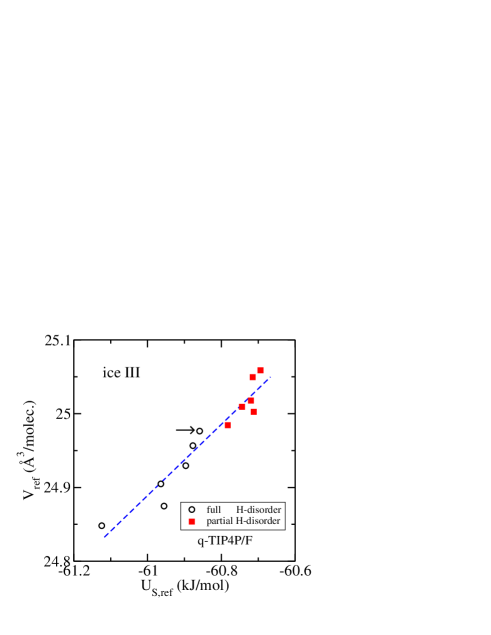
Figure 1: Minimum static energy and corresponding cell volume of randomly generated H-isomers of ice III. The H-isomers display either full (open circles) or partial (closed squares) H-disorder. The results correspond to the q-TIP4P/F model for a 324-molecule supercell. An arrow points to the H-isomer with full H-disorder and largest energy. This particular isomer is employed in the calculation of phase diagrams with different water models. The line is a linear fit to the data.

To this aim we have generated a random set of six H-isomers with full H-disorder and vanishing cell dipole moment for ice III. The result of their energy minimization with the flexible q-TIP4P/F potential is represented in Fig. 1. The volume, $V_{ref}$, and the corresponding minimized potential energy, $U_{S,ref}$, is displayed by open circles for each H-isomer. We note that the static energy, $U_{S,ref}$, of the six H-isomers spreads in an energy window of about 0.3 kJ/mol. The volume, $V_{ref}$, and the minimized potential energy, $U_{S,ref}$, are related in a nearly linear way. A second set of six random isomers with vanishing cell dipole moment has been generated by imposing the partial H-disorder encountered in the diffraction experiment of ice III.Lobban et al. (2000) The results of the energy minimization for the partially disordered structures are presented as closed squares in Fig. 1. All isomers having partial H-disorder display larger static energy than the isomers with full H-disorder.

Similar behavior to that shown in Fig. 1 is found if the minimization of the energy of the H-isomers is performed with the rigid TIP4P/2005 model. The main difference is that the dispersion of the $U_{S,ref}$ values increases slightly. Thus, two main conclusions can be derived from the results of the energy minimization in Fig. 1. The first is that the energetics associated to full versus partial H-disorder in ice III is incorrectly described by effective TIP4P-like models, i.e., full disorder is predicted to be more stable than partial one. Note that the configurational entropy $S_{H}$ will help to stabilize further the full disordered ice at any finite temperature, since $S_{H}$ in this case is larger than for the partial H-disorder. This behavior is in contradiction to the partial H-disorder experimentally found for ice III.Lobban et al. (2000) Our result is in line with the reported limitations of these effective potentials to reproduce the energetics of the H-bond rearrangement in the order-disorder transition of ice Ih-XI and VII-VIII.Buch et al. (1998); Singer and Knight (2011)

Our second conclusion is that the large dispersion in $U_{S,ref}$ obtained for ice III using cells with 324 molecules must affect the phase diagram whenever it is calculated with a single random H-isomer. The energy dispersion is caused by the proton disorder in the H-isomers. The sampling of this (large) dispersion of static cell energies with a single H-isomer can be considered the origin of a finite size effect. In the thermodynamic limit, the energy distribution of $U_{S,ref}$ should approximate a delta function centered at the energy corresponding to the most probable H-bond distribution. Therefore, the finite size effect caused by the insufficient sampling of the proton disorder (or the $U_{S,ref}$ energies) with a single H-isomer is expected to decrease as the size of the cell increases. An alternative way to reduce this finite size effect is to make a disorder averaging of the lattice energy of the employed ice cell. This point will be commented in Sec. VII.

In the case of ice Ih we have also generated a random set of six H-disordered structures. However, in this case the static energy, $U_{S,ref}$, of the H-isomers varies in a rather small energy window (of about 0.01 kJ/mol for the q-TIP4P/F model) and the corresponding volume changes by less than 0.04%. Thus, finite size effects related to the H-disorder are expected to be much lower in ice Ih than in ice III.

Table 1: Volume ($V_{ref}$) and static energy ($U_{S,ref}$) of the minimum energy configuration of the studied ice phases. The quantum QH results for the volume ($V_{0}$), static energy ($U_{S,0}$), zero-point energy ($U_{Z,0}$), and internal energy ($U_{0}$) are also given at $T=0$ and $P=0$. The data for ice III correspond to the H-isomer labeled by an arrow in Fig. 1. All results were derived with the q-TIP4P/F model. The last two columns show the difference with the data of ice II. $\left[V_{min},V_{max}\right]$ is the volume interval studied by the QHA for each phase.

$X$ (q-TIP4P/F)	Ih		II		III		$\Delta X$ (Ih-II)	$\Delta X$ (III-II)
$V_{ref}$ ($\textrm{\AA}^{3}/$molec.)	30.	96	24.	14	24.	99	6.82	0.85
$U_{S,ref}$ (kJ/mol)	-61.	98	-60.	84	-60.	86	-1.14	-0.02
$V_{0}$ ($\textrm{\AA}^{3}/$molec.)	32.	23	25.	11	25.	90	7.12	0.79
$U_{S,0}$ (kJ/mol)	-61.	74	-60.	60	-60.	77	-1.14	-0.17
$U_{Z,0}$ (kJ/mol)	68.	75	68.	08	68.	72	0.67	0.64
$U_{0}$ (kJ/mol)	7.	01	7.	47	7.	95	-0.46	0.47
$V_{min}$ ($\textrm{\AA}^{3}/$molec.)	29.	47	21.	75	22.	48
$V_{max}$ ($\textrm{\AA}^{3}/$molec.)	35.	05	27.	31	28.	22

A comparison of $V_{ref}$ and $U_{S,ref}$ calculated with the q-TIP4P/F model for ice Ih, II, and III are given in Tab. 1. The data for ice III correspond to the H-isomer labeled with an arrow in Fig. 1. The classical internal energy at zero temperature and pressure ($T=0$, $P=0$) is $U_{S,ref}$. The QH result in the quantum limit for the ice volume ($V_{0}$), static energy ($U_{S,0}$), and zero-point energy ($U_{Z,0}$) at $T=0$ and $P=0$ are also summarized in Tab. 1. The zero-point energy, $U_{Z,0}$, is calculated as

$$U_{Z,0}=\sum_{k}\frac{\hbar\omega_{k}(V_{0})}{2}\;.$$ (6)

Note that the zero-point energy of ice II is lower than that of ice Ih and III. In the quantum limit, the internal energy of the ice phases at $T=0$ and $P=0$ is

$$U_{0}=U_{S,0}+U_{Z,0}\;.$$ (7)

The ice structures studied in Tab. 1 have been analyzed also with the rigid TIP4P/2005 and TIP4PQ/2005 models. The corresponding results are presented in Tabs. 2 and 3. Note that the zero-point energy ($U_{Z,0}$) of the rigid models is about four times smaller than that of flexible water because of the neglect of intramolecular motion.

Table 2: Volume and energies of the studied ice phases as derived with the rigid TIP4P/2005 model at $T=0$ and $P=0$. The ice structures and variable labels are the same as those used in Tab. 1.

$X$ (TIP4P/2005)	Ih		II		III		$\Delta X$ (Ih-II)	$\Delta X$ (III-II)
$V_{ref}$ ($\textrm{\AA}^{3}/$molec.)	31.	34	24.	30	25.	26	7.04	0.96
$U_{S,ref}$ (kJ/mol)	-62.	99	-62.	13	-61.	86	-0.86	0.27
$V_{0}$ ($\textrm{\AA}^{3}/$molec.)	33.	20	25.	71	26.	76	7.59	1.05
$U_{S,0}$ (kJ/mol)	-62.	45	-61.	66	-61.	63	-0.79	0.03
$U_{Z,0}$ (kJ/mol)	16.	15	15.	10	16.	29	1.05	1.19
$U_{0}$ (kJ/mol)	-46.	30	-46.	56	-45.	33	0.26	1.23

Table 3: Volume and energies of the studied ice phases as derived with the rigid TIP4PQ/2005 model at $T=0$ and $P=0$. The ice structures and variable labels are the same as those used in Tab. 1.

$X$ (TIP4PQ/2005)	Ih		II		III		$\Delta X$ (Ih-II)	$\Delta X$ (III-II)
$V_{ref}$ ($\textrm{\AA}^{3}/$molec.)	30.	67	23.	85	24.	92	6.82	1.07
$U_{S,ref}$ (kJ/mol)	-68.	90	-67.	57	-67.	47	-1.33	0.10
$V_{0}$ ($\textrm{\AA}^{3}/$molec.)	32.	51	25.	16	26.	32	7.35	1.16
$U_{S,0}$ (kJ/mol)	-68.	35	-67.	11	-67.	24	-1.24	-0.13
$U_{Z,0}$ (kJ/mol)	17.	06	15.	91	17.	19	1.15	1.28
$U_{0}$ (kJ/mol)	-51.	30	-51.	20	-50.	05	-0.10	1.15

IV Flexible q-TIP4P/F model

In this section the QH phase diagram of ice Ih, II, and III is derived with the q-TIP4P/F model in both classical and quantum limits. Studied temperatures are in the interval [0,$300\;\mathrm{K}$] and pressures in the range [0, 0.35 GPa]. The calculation is done for each of the six random H-isomers of ice III having full H-disorder. A comparison to available TI simulations is provided in the classical limit.Habershon and Manolopoulos (2011a)

IV.1 Classical limit

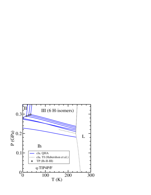
Figure 2: Phase diagram of ice Ih-II-III calculated with the q-TIP4P/F model in the classical limit. The full lines show the QH results. The QH calculation is done for six randomly chosen H-isomers having full H-disorder in a cell with 324 water molecules. The dotted lines are the classical TI results of Ref. Habershon and Manolopoulos, 2011a that include also the boundary with the liquid (L) phase. Circles show the position of the triple point (TP) for ice Ih-II-III.

The QH phase diagram of ice Ih, II, and III calculated in the classical limit is plotted in Fig. 2. Coexistence lines are displayed for each of the six studied H-isomers of ice III as continuous curves. We find that the finite size effect related to the H-disorder in ice III is important. In particular, the area where ice III is stable strongly depends upon the H-isomer. The dotted lines in Fig. 2 show the coexistence lines for ice Ih-III, Ih-liquid, and III-liquid as derived from the classical TI simulations of Ref. Habershon and Manolopoulos, 2011a with the q-TIP4P/F model. The coexistence line Ih-III is parallel to our QHA results.

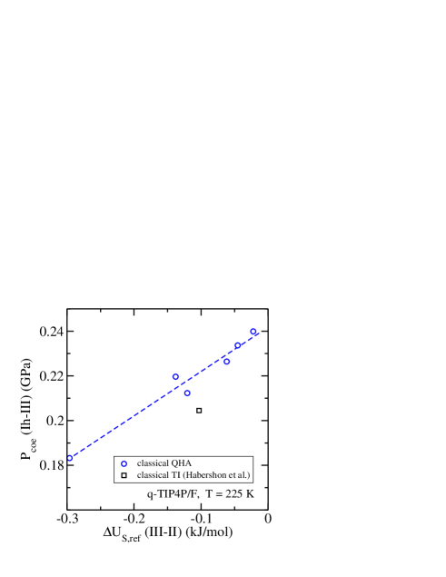
Figure 3: Coexistence pressure for ice Ih and III at 225 K as a function of the relative static energy of the H-isomers of ice III. The static energy of ice II has been taken as zero of the energy scale. Circles are results derived by the QHA using the q-TIP4P/F model. The square is the result of Ref. Habershon and Manolopoulos, 2011a based on the TI method with the same water potential. The line is a linear fit to the QH data.

For the various H-isomers, the ice Ih-III phase boundary is shifted by a nearly constant pressure. The dispersion of the static energy, $U_{S,ref}$, is the factor responsible for the different phase behavior of the H-isomers. Vibrational contributions to the free energy are however similar. The coexistence pressure for the Ih-III transition at the temperature of $T=225$ K is represented in Fig. 3 as a function of the relative static energy, $\Delta U_{S,ref}$, of the H-isomers of ice III. The relative energy is calculated with respect to the minimum potential energy of ice II, to allow for a comparison to available literature data.Habershon and Manolopoulos (2011a) The coexistence pressure varies in the interval 0.18-0.24 GPa at 225 K. There appears an approximate linear relation between the coexistence pressure and the static energy of the ice III isomer. The coexistence pressure reported using TI simulations deviates by less than 0.02 GPa (about 8%) from the linear fit based upon the QH results. This small deviation suggests that the QHA is reasonably realistic even at this relatively high temperature ($T=225$ K). The difference between the QHA and the TI simulations is caused by the presence of anharmonic effects not included in the QHA and also by the use of different H-isomers in both calculations. Unfortunately it is not possible to quantify the separate influence of both factors.

An interesting result from our QH phase diagram is that, for cells with 324 molecules, ice II may be either stable at low $T$ or unstable at all temperatures in the classical limit of the q-TIP4P/F water model. We find in Fig. 2 that ice II is unstable in the whole ($T,P$) region if the phase diagram is calculated with any of the three most stable H-isomers of ice III. Thus, the stability of ice II is determined by the static energy, $U_{S,ref}$, of the H-isomer of ice III.

Some differences in the phase diagrams calculated with TIP4P-like models might be caused by the differences in the static energy, $U_{S,ref}$, of the single H-isomer chosen to represent ice III. For example, the classical phase diagram for the rigid TIP4P model was calculated with a H-isomer of ice III with partial H-disorder.Sanz et al. (2004) We have seen in Fig. 1 that partial H-disorder is less stable (it has higher energy) than full H-disorder for TIP4P-like models. Thus, this choice helps to increase the stability region of ice II. On the contrary, the phase diagram for the flexible q-TIP4P/F model was calculated with full H-disorder for ice III. Here the increased stabilization of ice III (see Fig. 1) plays an important role for the reported instability of ice II.Habershon and Manolopoulos (2011a) Our QH calculation strongly suggests that the ice II instability is not a deficiency of the q-TIP4P/F model, but a finite size effect related to the particular H-isomer randomly selected for the simulation.

We turn now to the calculation of the QH phase diagram of ice Ih, II, and III for the quantum limit of the q-TIP4P/F model. In this case there are quantum TI results for the melting of ice Ih at atmospheric pressure,Ramírez and Herrero (2010); Habershon and Manolopoulos (2011b) but not for the coexistence between different ice phases.

IV.2 Quantum limit

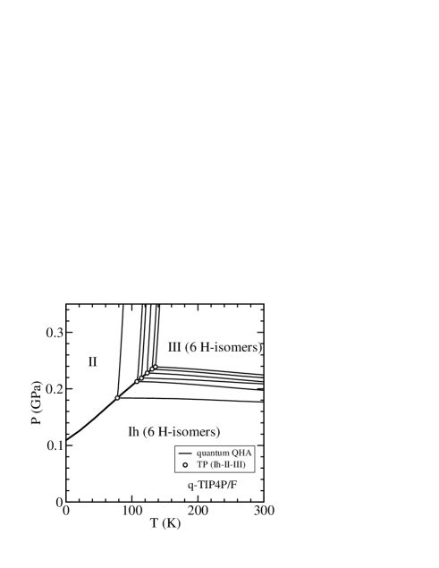
Figure 4: QH phase diagram of ice Ih-II-III calculated with the q-TIP4P/F model in the quantum limit. The multiple coexistence lines II-III and Ih-III show the results for the six studied H-isomers of ice III. The phase boundary Ih-II is a plot of six superimposed lines, each one calculated with a different random H-isomer of ice Ih. Circles show the position of the triple point (TP) for the ice phases.

The QH phase diagram of ice Ih, II, and III in the quantum limit is plotted in Fig. 4. Finite size effects related to proton disorder are very important for ice III ($N=324$). As in the classical limit, this effect is related to the differences in the static energy, $U_{S,ref}$, of the H-isomers of ice III. Vibrational contributions to the free energy are however similar, and then the coexistence lines calculated for the ice III isomers are nearly parallel.

In contrast, the QHA reveals that finite size effects related to H-disorder are vanishingly small for ice Ih ($N=288$). The coexistence line Ih-II was calculated for each of the six randomly generated H-isomers of ice Ih. In this case, the six calculated Ih-II phase boundaries appear superposed as a unique line at the scale of the figure. The coexistence lines Ih-III have been displayed for a single H-isomer of ice Ih.

Ice II is always a stable phase in the quantum phase diagram independently of the employed H-isomer of ice III. A triple point Ih-II-III appears for all studied H-isomers, in contrast to the classical results in Fig. 2. The triple point temperature, $T_{TP}$, is found in an interval 75-136 K depending upon the H-isomer of ice III. The triple point pressure, $P_{TP}$, appears in the interval 0.18-0.24 GPa. The magnitude of these intervals provides a quantitative estimation of the influence of the finite size effect of the proton disorder of ice III in the calculated phase diagram. We find that both quantities ($T_{TP},P_{TP}$) show a linear dependence as a function of the static energy, $U_{S,ref}$, of ice III, in a way very similar to that shown in Fig. 3 for the coexistence pressure between ice Ih and III.

IV.3 Comparison of quantum and classical limits

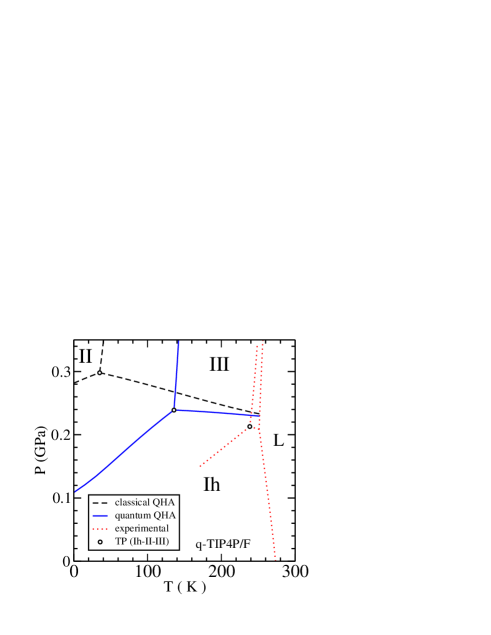
Figure 5: Comparison of the QH phase diagram of ice Ih, II, and III in the classical and quantum limits. Dotted lines correspond to experimental data from Ref. Dunaeva et al., 2010 that include the liquid (L) phase. Results derived with the q-TIP4P/F model. The calculation was performed with the H-isomer of ice III labeled with an arrow in Fig. 1. Circles show the position of the triple point for ice Ih-II-III.

The quantum and classical limits of the QH phase diagram for the q-TIP4P/F model are compared in Fig. 5. The H-isomer of ice III indicated by an arrow in Fig. 1 has been arbitrarily chosen for this comparison. The static energy of this H-isomer is the closest one to that of partial H-disorder structures. The most conspicuous quantum effect is the increased stability of ice II. The triple point Ih-II-III is found classically at (35 K, 0.3 GPa), while the quantum limit is (136 K, 0.24 GPa), i.e. a shift of about 100 K and -0.06 GPa due to the consideration of quantum vibrational effects. The experimental boundaries in this region of the phase diagram are shown in Fig. 5 by dotted lines. The experimental triple point Ih-II-III is found at (239 K, 0.21 GPa).Dunaeva et al. (2010)

IV.3.1 Coexistence Ih-II

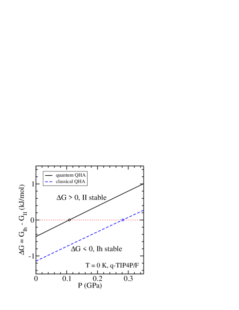
Figure 6: Gibbs free energy difference of ice Ih and II as a function of $P$ at $T=0$ K. Coexistence conditions are labeled by open symbols ($\Delta G=0$). Results derived with the q-TIP4P/F model in both classical and quantum limits.

In the quantum limit, ice II occupies a large portion of the region of stability found classically for ice Ih. Therefore, the coexistence line Ih-II is shifted to lower pressures with respect to the classical one (see Fig. 5). The Gibbs free energy difference between ice Ih and II,

$$\Delta G=G_{Ih}-G_{II}\;,$$ (8)

is plotted in Fig. 6 as a function of the pressure at $T=0$ K. The zero temperature condition implies that

$$\Delta G=\Delta U+P\Delta V\;.$$ (9)

The plot of $\Delta G$ in Fig. 6 is nearly linear in $P$. This fact, in the light of Eq. (9), implies that both $\Delta U$ and $\Delta V$ vary slowly with $P$ in the studied pressure interval.

The main difference between the quantum and classical result for $\Delta G$ is the value of the ordinate at the origin, $\Delta U_{0}$. Fig. 6 shows that in the classical limit

$$\Delta U_{0,cla}=-1.14\;\mathrm{kJ/mol}\left(\equiv\Delta U_{S,ref}\right)\;,$$ (10)

a value that corresponds to the difference in the static energies, $U_{S,ref},$ of ice Ih and II (see Tab. 1). In the quantum limit the ordinate at the origin is

$$\Delta U_{0}=-0.46\;\mathrm{kJ/mol}\left(\equiv\Delta U_{S,0}+\Delta U_{Z,0}\right)\;.$$ (11)

The quantum result differs from $\Delta U_{0,cla}$ by an energy increment that essentially corresponds to the difference in the zero-point energy, $U_{Z,0},$ of ice Ih and II at $T=0$ and $P=0$. The data in Tab. 1 show that

$$\Delta U_{Z,0}=U_{Z,0,Ih}-U_{Z,0,II}=0.67\;\mathrm{kJ/mol}\;,$$ (12)

i.e., the zero-point energy of ice II is 0.67 kJ/mol lower than that of ice Ih. This is the physical reason for the quantum shift in the coexistence pressure of the Ih-II transition (abscissa of the open circles in Fig. 6) and the origin of the increased stabilization of ice II in the quantum phase diagram.

Table 4: Average of the wavenumbers obtained with the q-TIP4P/F model for the volume $V_{0}$ of the studied ices. $V_{0}$ is the equilibrium volume in the quantum limit at $T=0$ and $P=0$. The last two columns show the ratio of the wavenumbers with respect to the data of ice II.

$\overline{\omega}_{k}$ (cm${}^{-1})$	Ih	II	III	Ih/II		III/II
$3N$ translations	186	176	189	1.	06	1.	07
$3N$ librations	747	684	738	1.	09	1.	08
$N$ bending	1684	1673	1682	1.	01	1.	01
$2N$ stretching	3506	3565	3512	0.	98	0.	99

Why is the $U_{Z,0}$ of ice II lower than that of ice Ih? $U_{Z,0}$ is proportional to the average of the vibrational frequencies, $\overline{\omega}_{k}$, of the ice cell [see Eq. (6)]. In Tab. 4, the average of translational, librational, bending and stretching modes is presented for the equilibrium cells of the ice phases. We observe that the largest difference in $\overline{\omega}_{k}$ between ice Ih and II is due to the librational modes, that are about 10% lower in ice II. The stretching modes show a competing behavior in the sense that they are larger for ice II. But the overall effect of all modes is the reduction of the zero-point energy of ice II in comparison to ice Ih by about 0.67 kJ/mol (1%). We can anticipate that for rigid water models this competing mechanism between librational and stretching modes is absent. Thus, the stabilization of ice II in the quantum phase diagram of rigid models should be even larger than in the flexible one.

IV.3.2 Coexistence II-III

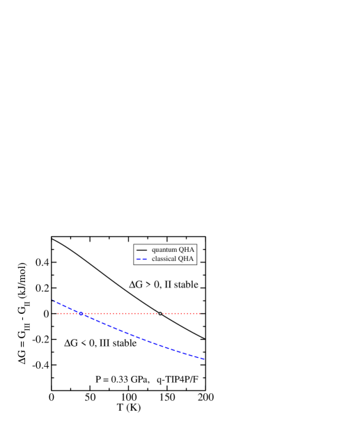
Figure 7: Gibbs free energy difference between ice III and II as a function of $T$ at $P=0.33$ GPa. Coexistence conditions are labeled by open symbols ($\Delta G=0$). Both classical and quantum limits were derived with the q-TIP4P/F model for the H-isomer of ice III labeled with an arrow in Fig. 1.

The Gibbs free energy difference between ice III and II is plotted as a function of the temperature in Fig. 7. Both classical and quantum QHA limits are displayed at a constant pressure of $P=0.33$ GPa. The coexistence temperature in the quantum limit is shifted by about 100 K toward higher temperatures, i.e., quantum effects play an important role in the stabilization of ice II. The zero-point energies in Tab. 1 show that $U_{Z}$ of ice II is significantly lower (about 0.6 kJ/mol) than that of ice III. The slope of the $\Delta G$ curves in Fig. 7 is always negative

$$\frac{\partial\left(\Delta G\right)}{\partial T}=-\Delta S=S_{II}-S_{III}<0\;,$$ (13)

which is consistent with the larger entropy of ice III due to its H-disorder. At a given temperature the slope of the quantum $\Delta G$ curve is larger (in absolute value) than in the classical result. This implies that the excess of entropy of ice III, with respect to ice II, is larger in the quantum limit, i.e., the quantum vibrational entropy contributes to stabilize ice III. Nevertheless, the overall quantum effect in $\Delta G$ implies a strong stabilization of ice II with respect to ice III, as a consequence of its lower zero-point energy.

V Rigid TIP4P/2005 model

The QH phase diagram of ice Ih, II, and III with the rigid TIP4P/2005 potential has been calculated using the same H-isomers as those employed for the q-TIP4P/F study in Fig. 5. Differences in the results should be attributed to the potential models (flexible versus rigid) and not to effects related to the selected H-isomers.

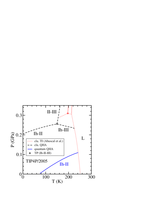
Figure 8: Comparison of the QH phase diagram of ice Ih, II, and III in the classical and quantum limits. Dotted lines correspond to the classical TI simulations of Ref. Abascal and Vega, 2005 that include the liquid (L) phase. These results were derived with the TIP4P/2005 model. Ice III is modeled with the same H-isomer as that employed in Fig. 5 for the q-TIP4P/F model. Circles show the position of the triple point for ice Ih-II-III.

The classical and quantum QH phase diagrams are presented in Fig. 8 as dashed and continuous curves, respectively. The phase diagram reported for the TIP4P/2005 model by classical TI simulations is shown by dotted lines. In the last case the coexistence with the liquid phase is also given. There are several aspects to be commented. First is the comparison between the classical QHA and the TI results. The coexistence lines between the ice phases are nearly parallel in both calculations. We recall that the slope of the coexistence lines is determined by the Clausius-Clapeyron relation

$$\frac{dP_{coe}}{dT_{coe}}=\frac{\Delta H}{T_{coe}\Delta V}=\frac{\Delta S}{\Delta V}\;,$$ (14)

where $\Delta H$ is the enthalpy difference (latent heat) between the two phases at equilibrium. It has been shown earlier that the QHA provides a realistic approximation for the enthalpy and volume of ice Ih, II, and III in a broad ($T,P$) interval.Ramírez et al. (2012) Therefore, the QHA shows a reasonable overall agreement to the classical TI results for the slopes of the coexistence lines. The largest deviation between the QH and TI slopes is found for the Ih-II transition at temperatures close to the triple point, where the slope of the QHA is lower. The larger stability region of ice III in the QHA is likely due to the finite size effect related to the different H-ordering of the studied H-isomers, although the approximate treatment of anharmonic effects by the QHA may be also the origin of this behavior.

The consideration of quantum vibrational effects changes dramatically the QH phase diagram. The main quantum effect is the stabilization of ice II. It has two important consequences. The first is that ice II becomes the stable phase at low temperatures even at $P=0$. The second is that ice III disappears as stable phase in the displayed region of the phase diagram. Both facts imply that the quantum QH phase diagram becomes in strong disagreement to experimental facts, as opposed to the classical one.

In the case of the TIP4P/2005 model there are not quantum TI results available for comparison. Nevertheless the QH prediction that ice II becomes the stable low temperature phase agrees with the quantum path integral simulations of ice Ih and II in Ref. McBride et al., 2009. The explanation given for this behavior was that the TIP4P/2005 model is parameterized to be used in a classical limit. The combination with quantum simulations implies some kind of overcounting of quantum effects that leads to unphysical results.

It is interesting to analyze the physical reason for the larger stabilization of ice II in the quantum phase diagram of Fig. 8 (rigid model) in comparison to Fig. 5 (flexible model). At $T=0$ and $P=0$ the shift in the coexistence pressure of ice Ih-II in the classical and quantum limits is proportional to the difference in the zero-point energy, $\Delta U_{Z,0}$, between both phases. For TIP4P/2005 we get (see Tab. 2 )

$$\Delta U_{Z.0}=U_{Z,0,Ih}-U_{Z,0,II}=1.05\;\mathrm{kJ/mol}\;,$$ (15)

i.e., the zero-point energy of ice II is more than 1 kJ/mol lower than that of ice Ih. This stabilization is about 50% larger than that of the flexible model [see Eq. (12)]. This fact is a consequence of the absence in a rigid model of competing contributions of librational and stretching modes to $\Delta U_{Z,0}$, as discussed in Subsec. IV.3.1. In conclusion, the stabilization of ice II by its lower zero-point energy is larger for the rigid model than for the flexible one. As a consequence ice II becomes the stable phase at low temperature and ice III is unstable in the quantum limit of the TIP4P/2005 model (see Fig. 8).

A last remark on the comparison of the QH phase diagrams of the rigid and flexible models. The most realistic results are obtained in the quantum limit for the flexible model (see Fig. 5), but in the classical limit for the rigid model (see Fig. 8). The models were parameterized to be used in either quantum (the flexible one)Habershon et al. (2009) or classical simulations (the rigid one).Abascal and Vega (2005) Thus, the best result correlates in each case with the conditions where the model was parameterized.

VI Rigid TIP4PQ/2005 model

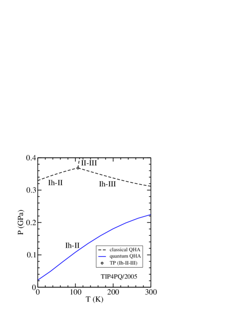
Figure 9: Comparison of the QHA phase diagram of ice Ih, II, and III in the classical and quantum limits. Results derived with the TIP4PQ/2005 model. Ice III is modeled with the same H-isomer as that employed in Fig. 8 for the TIP4P/2005 model. A circle shows the position of the triple point for ice Ih-II-III in the classical limit.

The rigid TIP4PQ/2005 model differs from TIP4P/2005 by an increase of about 4% in the point charges, i.e., the parameter $q_{H}$ is the only one that changes from 0.5564 $e$ to 0.5764 $e$.McBride et al. (2009) The QH phase diagram of ice Ih, II, and III for the rigid TIP4PQ/2005 potential has been calculated with the same H-isomers as those used in the studies shown in Fig. 5 (q-TIP4P/F) and Fig. 8 (TIP4P/2005). The results for TIP4PQ/2005 are displayed in Fig. 9.

We observe that the QH diagrams in Figs. 8 and 9 are qualitatively similar. In the classical case, there appears a triple point for the ices Ih-II-III. However, in the quantum limit, ice III is unstable and the phase diagram displays only the ice Ih-II transition. Another similarity of both phase diagrams is that the coexistence lines in Figs. 8 and 9 are nearly parallel.

The change in the point charges modifies the static energy, $U_{S,ref},$ of the ice phases (see Tabs. 2 and 3). This translates into a shift of the coexistence lines calculated with both rigid models. For example, in the quantum limit the transition Ih-II appears at higher pressures for TIP4PQ/2005, so that ice Ih becomes the stable low temperature phase (see Fig. 9). This result is in agreement with the path integral simulations of the TIP4PQ/2005 model in Ref. McBride et al., 2009.

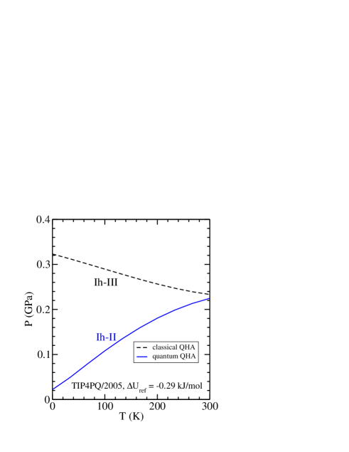
Figure 10: Comparison of the QH phase diagram of ice Ih, II, and III in the classical and quantum limits. Results derived with the TIP4PQ/2005 model. The results differ from those in Fig. 9 by an additional stabilization of ice III by a constant energy shift given by $\Delta U_{ref}$.

Classical and quantum phase diagrams of water, derived by TI simulations with the TIP4PQ/2005 model, have been reported recently.McBride et al. (2012) The results differ markedly from our QHA. We believe that the main reason of discrepancy is the finite size effect in the value of the static energy, $U_{S,ref}$, of ice III. As a check of this hypothesis, we have repeated our QHA calculation of the TIP4PQ/2005 phase diagram by shifting the internal energy of ice III by a constant amount. All other model parameters remain unchanged (i.e., static energies of ice Ih and II, and the vibrational properties of the three ice phases). We have analyzed the effect of setting the static energy of ice III as

$$U_{S,new}(V)=U_{S}(V)+\Delta U_{ref}\;,$$ (16)

where $\Delta U_{ref}$ is a constant energy shift. The QH phase diagram for $\Delta U_{ref}=0$ was displayed in Fig. 9. The phase diagrams derived for $\Delta U_{ref}=-0.29$ kJ/mol and $\Delta U_{ref}=-0.47$ kJ/mol are displayed in Figs. 10 and 11, respectively. The differences between these phase diagrams are caused by the artificial stabilization of ice III by the constant energy $\Delta U_{ref}$. Note that the selected energy shifts are in the order of the dispersion of $U_{S,ref}$ represented in the abscissa of Fig. 1 for the q-TIP4P/F model.

In the quantum limit, the phase diagram calculated with $\Delta U_{ref}=-0.29$ kJ/mol (Fig. 10), is identical to that shown for $\Delta U_{ref}=0$ (Fig. 9). The coexistence Ih-II is the only transition. The additional stabilization of ice III is not large enough to make it stable in the quantum limit. However, it does change drastically the classical limit of the phase diagram. Ice III becomes more stable than ice II in the whole region, and the classical phase diagram loses its triple point and now displays only the ice Ih-III transition. Note that for $\Delta U_{ref}=-0.29$ kJ/mol, the triple point Ih-II-III is missing in both classical and quantum limits.

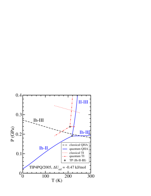
Figure 11: Comparison of the QH phase diagram of ice Ih, II, and III in the classical and quantum limits. Results derived with the TIP4PQ/2005 model. The results differ from those in Fig. 9 by an additional stabilization of ice III by a constant energy shift given by $\Delta U_{ref}$. Dotted (dashed-dotted) lines correspond to the classical (quantum) TI simulations of Ref. McBride et al., 2012. Circles show the position of the triple point for ice Ih-II-III.

Imposing a larger stabilization to ice III ($\Delta U_{ref}=-0.47$ kJ/mol), we obtain the QHA phase diagram shown in Fig. 11. In this plot we have represented also the classical and quantum phase diagrams for ice Ih, II, and III calculated by TI simulations in Ref. McBride et al., 2012. We observe that this additional stabilization brings the QHA in reasonable agreement to the TI results reported for this model. Now a triple point Ih-II-III is observed in the quantum limit, while the transition Ih-III is the only line in the classical case. Furthermore, we note that the slopes of the coexistence lines predicted by the QHA are in reasonable agreement to the TI results.

The sequence of phase diagrams shown in Figs. 9, 10, and 11 provides a vivid illustration of the dramatic changes in the ice phase diagram as a function of the stability of the employed H-isomer of ice III.

VII Average over proton disorder

In this Section we comment on the necessity of performing some form of proton disorder average, at least for ice III, prior to the calculation of the phase diagram. Assuming that the number of H-isomers for an ice cell is $M$, the canonical partition function of the ice phase can be expressed as

$$e^{-\beta F}=\sum_{i=1}^{M}e^{-\beta(U_{S,i}+F_{v,i})}\;,$$ (17)

where $U_{S,i}$ and $F_{v,i}$ are the static energy and the vibrational free energy of i’th H-isomer. Note that many of the $M$ H-isomers might be energetically degenerate as a consequence of the lattice symmetry. Eq. (17) is the formally correct way to average over the proton disorder of the ice phase. It has been applied to study order-disorder transitions of ice phases using small units cells.Singer and Knight (2011) Obviously for large unit cells the total number $M$ of H-isomers grows in such a way that the application of Eq. (17) becomes an impossible task.

The alternative for large unit cells is the use of Eq. (1), which is applied to a single H-isomer selected randomly from the set of $M$ available ones.Sanz et al. (2004); Abascal and Vega (2005); McBride et al. (2012); Habershon and Manolopoulos (2011a) Note that in this equation the average over proton disorder is introduced ad hoc by the term with the proton disorder entropy $S_{H}$. An implicit assumption in Eq. (1) is that the cell is so large that the static energy, $U_{S},$ and the vibrational free energy, $F_{v}$, of the single H-isomer do not require any further average over the proton disorder. This assumption is correct in the thermodynamic limit as the relative fluctuation of thermodynamic quantities is expected to decrease as $1/\sqrt{N}$.

However, we have shown that, for typical cell sizes used in simulations, the fluctuation of $U_{S}$ for ice III is far from its ideal thermodynamic limit. Therefore some form of proton disorder averaging of $U_{S}$ is necessary. A computational feasible proposal is to average only the term that shows the largest fluctuation as a function of the H-disorder, which is the potential energy of the reference cell $U_{S,ref}$ associated to the chosen H-isomer. Thus, a simple proposal to average over proton disorder is to modify the static energy in Eq. (1) by

$$U_{S,ave}(V)=U_{S}(V)+\Delta U_{ave}\;.$$ (18)

$\Delta U_{ave}$ here is a constant energy shift that modifies the stability of the single selected H-isomer of ice III by an amount determined by the average $\overline{U}_{S,ref}$ calculated over a random set of H-isomers, i.e.,

$$\Delta U_{ave}=\overline{U}_{S,ref}-U_{S,ref}\;.$$ (19)

Note that the proposed disorder averaging can be applied to the calculation of phase diagrams either by the QHA or by TI simulations.

The average of $U_{S,ref}$ over the set of six random H-isomers of ice III with full H-disorder studied in this work gives $\overline{U}_{S,ref}=-60.96\pm 0.04$ kJ/mol for the q-TIP4P/F model. We estimate that the error of the mean value, $\overline{U}_{S,ref}$, should be as low as 0.01 kJ/mol for a reasonable convergence over the proton disorder. Then the size of our random sampling should be increased by a factor of 16 to reduce our estimated error to this limit, i.e., for an ice III cell with 324 molecules one should increase the sampling of $U_{S,ref}$ to about 100 H-isomers. By using larger units cells, e.g., a $4\times 4\times 4$ supercell with 768 water molecules, the number of required H-isomers to obtained a converged value of $\overline{U}_{S,ref}$ should be lower than this. However, in terms of computational efficiency, the lower number of H-isomers may be overcompensated by the higher computational cost in the minimization of the cell energies.

In the case of the partially disordered ice III we get $\overline{U}_{S,ref}=-60.73\pm 0.01$ kJ/mol for our set of six random H-isomers with the q-TIP4P/F model. This value has achieved already the desired convergence. A last comment is that the proton disorder entropy $S_{H}$ for partially disordered phases is lower than the Pauling estimate in Eq. (2). The estimation of $S_{H}$ for the fractional H-occupancies experimentally determined for ice III amounts to about 90% of the Pauling result. This entropy lowering has a significant influence in the phase diagram.MacDowell et al. (2004) Numerical methods for the estimation of the proton disorder entropy of partially H-disordered phases can be found in Refs. MacDowell et al., 2004; Berg and Yang, 2007.

VIII Conclusions

In this work we have presented a detailed study of the phase diagram of ice Ih, II, and III calculated with the QHA and TIP4P-like models. Several advantages of the QHA are worth to be mentioned: its computational cost is low, it is free from the statistical errors inherent to any numerical simulation, it can be applied to both classical and quantum limits, and the most accurate results are expected in the low temperature limit, where anharmonicities are lower. These advantages make the QHA an appropriate option to study finite size effects that can become prohibitively expensive in numerical (Monte Carlo or molecular dynamics) simulations.

The effect of proton disorder in the phase diagram of TIP4P-like models has been a focus of our study. We have found that for the typical cell sizes employed in computer simulations, the finite size effect of H-disorder in ice Ih is very small. However, this effect is very large for ice III, so that the transitions II-III and Ih-III are strongly affected by it. The physical reason for this behavior is that the static energy of ice III may change by an amount of several tenths of kJ/mol depending on the considered H-configuration. Thus a randomly selected ice III structure makes the calculated phase diagram affected by an uncontrolled factor that can be highly significant for the final result. Crystallographic data of ice Ih and III reveal significant differences as a consequence of the larger structural complexity of ice III. As example, ice Ih is a network of hexagon rings of O-atoms, while in ice III there appear five-, seven, and eight-members rings. The tetragonal O-O-O angles deform from the ideal value of about 109^∘ in ice Ih into angles between 80^∘ and 140^∘ in ice III.Lobban et al. (2000) Thus the large finite size effect related to the H-disorder in ice III, in comparison to ice Ih, seems to correlate with its increased structural complexity. We have discussed the necessity of performing a disorder average of the lattice energy in order to reduce this effect.

Another aspect related to the H-disorder in ice III is that TIP4P-like models predict that full H-disorder is more stable than partial H-disorder. However, this result is against the data derived from diffraction experiments of ice III.Lobban et al. (2000) A phase diagram derived with ice III having partial H-disorder may be significantly different from that derived with full H-disorder, as a consequence of the differences in their static energies.

These findings allows us to rationalize previously contradictory results of phase diagrams calculated with TIP4P-like potentials. A significant example was the reported instability of ice II in the classical limit of the flexible q-TIP4P/F model.Habershon and Manolopoulos (2011a) This fact contrasts with the stability of ice II reported with rigid TIP4P and TIP4P/2005 models.Sanz et al. (2004); Abascal and Vega (2005) Our QH results show that the stability of ice II strongly depends upon the H-configuration of the chosen ice III isomer. The fact that ice III has been described either with partialSanz et al. (2004) or full H-disorderHabershon and Manolopoulos (2011a); McBride et al. (2012) makes difficult the comparison of phase diagrams with different models. It is not easy to discriminate from the reported simulations the effects due to the variable stability of the ice III isomers from those caused by the different water models.

The QH phase diagram of ices Ih-II-III for the q-TIP4P/F, TIP4P/2005 and TIP4PQ/2005 effective potentials has been able to reproduce qualitatively most features that had been previously studied by TI in both classical and quantum simulations. Our results are obtained using the same H-isomers for the three TIP4P-like models, allowing for an easier interpretation of the differences encountered in the phase diagrams. We have found that for the flexible model (q-TIP4P/F) the triple point Ih-II-III is shifted in the quantum limit by 100 K and -0.06 GPa with respect to the classical one. This effect is very large, specially in the temperature. Its physical origin is related to the lower zero-point energy of ice II, when compared to that of ice Ih and III. This fact translates in an increased stability of ice II when vibrational quantum effects are considered. The average frequency of molecular librations in the H-bond network are nearly 10% smaller in ice II than in the other ice phases. This causes a significant reduction of the zero-point energy. Interestingly, the intramolecular stretching modes of ice II are predicted at higher frequencies than those in ice Ih and III. This anticorrelation between libration and stretching modes has been often stressed in the literature, i.e., any factor that shifts librational frequencies in one direction acts also modifying the stretching frequencies in the opposite one.Pamuk et al. (2012) We find as net effect that librational modes dominate over stretching ones, leading to the stabilization of ice II by its lower zero-point energy.

The main difference between the QH phase diagrams obtained by the flexible and rigid models is associated to the absence of anticorrelation between H-bond librations and O-H stretchings in the rigid models. Obviously intramolecular bonds are frozen for rigid water. As a consequence, the stabilization of ice II by its zero-point energy is larger for the rigid models (TIP4P/2005, TIP4PQ/2005) than for the flexible one (q-TIP4P/F). It may be even so large that ice II becomes the stable phase at low temperatures. This result has been reported by quantum path integral simulations with the TIP4P/2005 potential in Ref. Abascal and Vega, 2005 and is also reproduced by our QHA. Another effect related to the large stabilization of ice II is that this phase may occupy the stability region of ice III in the quantum limit of the rigid models. Then the triple point Ih-II-III does not appear in the quantum phase diagram. This unphysical behavior, as displayed in the quantum phase diagrams of Figs. 8 and 9, can be avoided if the H-isomer of ice III is particularly stable, as was shown in the phase diagram of Fig. 11.

The present work can be extended along several directions. An obvious one is the analysis of the phase diagram of other ice phases with the flexible q-TIP4P/F model as well as the study of finite size effects in the proton disorder of other phases, as ice V, VI, and VII. A second aim is the use of DFT to avoid the limitations of the empirical potentials, in particular with respect to the energetics associated to proton rearrangements in ice phases.