Semi-classical theory for quantum quenches in the O(3) non-linear sigma model

Stefano Evangelisti1,2 1 The Rudolf Peierls Centre for Theoretical Physics, University of Oxford - Oxford OX1 3NP, United Kingdom 2 Department of Physics, University of Bologna and INFN, Via Irnerio 46, 40136, Bologna, Italy
Abstract

We use the semi-classical approach to study the non-equilibrium dynamics of the O(3) non-linear sigma model. For a class of quenches defined in the text, we obtain the order-parameter dynamical correlator in the thermodynamic limit. In particular we predict quench-dependent relaxation times and correlation lengths. The approach developed for the O(3) non-linear sigma model can also be applied to the transverse field Ising chain, where the semi-classical results can be directly compared to both the exact and the numerical ones, revealing the limits of the method.

1 Introduction

The out-of-equilibrium physics of many-body systems has attracted a lot of interest in recent years, not least because of the experimental realizations of ultracold atomic gases in optical lattices [1, 2, 3, 4, 5, 6]. These experiments have observed the dynamics of many-body systems on a long time scale after a quantum quench, finding essentially unitary time-evolution. In three-dimensional systems fast relaxation towards a thermal steady state has been observed. On the contrary, in quasi-one-dimensional systems the relaxation process is normally much slower and leads to a peculiar non-thermal stationary state [2]. These results have led to a huge theoretical push [3, 4, 5, 6, 7, 8, 9, 10, 11, 12, 13, 14, 15, 16, 17, 18, 19, 20, 21, 22, 23, 24, 25] to address fundamental questions such as whether there is an asymptotic stationary state, and, if it exists, which ensemble characterizes it. The belief is that observables of non-integrable systems effectively thermalize, which implies that their stationary state is characterized by a thermal Gibbs ensemble. Numerical works on non-integrable systems confirm this expectation, even if some contradictory results point out that some issues have not been completely understood yet [19, 20, 21, 26]. On the other hand, in integrable systems, because of the existence of local integrals of motion, the stationary state is expected to be described by a generalized Gibbs ensemble (GGE), where each mode associated with a conseved quantity is characterized by its own temperature. So far results on integrable systems have been focussed on free fermion models, such as the transverse field Ising chain and the quantum XY chain [27, 28, 29, 30, 31, 32, 33, 34, 35, 36, 37, 38, 39, 40, 41, 42, 43, 44].
For the transverse field Ising chain in thermal equilibrium Sachdev and Young first introduced a semi-classical description of the physical properties of the model in terms of ballistically moving quasi-particles [45]. This approach turned out to be incredibly accurate in predicting the temperature dependence of correlation length, relaxation time and in general to compute the order-parameter two point function in the ferromagnetic and paramagnetic phases. For global quenches this technique has been used to describe the dynamics of the transverse field Ising chain and the quantum XY model, with great accuracy [30, 37, 39, 44]. In these works quantitative features of the relaxation process have been explained with a quasi-particle picture, which had been introduced before in particular to study the evolution of the entanglement entropy [32, 46, 47, 48]. In practice the quench injects an extensive amount of energy into the system, which creates quasi-particles homogeneously in space, that then move ballistically with constant velocity. Because of momentum conservation, these quasi-particles are created in pairs with opposite momenta and are quantum entangled (within each pair). Their dynamics can be treated classically as long as they do not collide. But since collisions are unavoidable in one dimension, every scattering process has to be treated quantum mechanically. We shall use this semi-classical approach to calculate the dynamical correlation functions analytically for the O(3) non-linear sigma model. The dynamics of this model have already been studied at finite temperature in equilibrium [49, 50], where the order-parameter correlation function shows a universal form. Here we shall study its behaviour after a quantum quench, preparing the system in a state which is not an eigenstate of the Hamiltonian. In addition a section will be dedicated to the case of the transverse field Ising chain, whose order-parameter two-point correlation function can be derived straightforwardly from the general one obtained for the O(3) non-linear sigma model.
The paper is organized as follows: first we introduce the model and the general form of the initial states we shall consider throughout the whole article, before introducing and commenting the main result of the paper, concerning the O(3) non-linear sigma model. Then we describe the basic ideas behind the semi-classical technique and see in detail how to apply them in the present case.

2 The Model

Let us start by considering the one-dimensional Oโ€‹(3)๐‘‚3O(3) quantum rotor chain, which is described by the following Hamiltonian:

H^rotor=Jโ€‹g2โ€‹โˆ‘iL^i2โˆ’Jโ€‹โˆ‘in^iโ€‹n^i+1,superscript^๐ปrotor๐ฝ๐‘”2subscript๐‘–superscriptsubscript^๐ฟ๐‘–2๐ฝsubscript๐‘–subscript^๐‘›๐‘–subscript^๐‘›๐‘–1\hat{H}^{\rm rotor}=\frac{Jg}{2}\sum_{i}\hat{L}_{i}^{2}-J\sum_{i}\hat{n}_{i}\hat{n}_{i+1}, (1)

where n^isubscript^๐‘›๐‘–\hat{n}_{i} is the position operator of the rotor on site i=1,โ€ฆ,L๐‘–1โ€ฆ๐ฟi=1,\dots,L with the constraint n^i2=1superscriptsubscript^๐‘›๐‘–21\hat{n}_{i}^{2}=1โ€‰โˆ€isubscriptfor-all๐‘–\forall_{i}, and L^i=n^iร—p^isubscript^๐ฟ๐‘–subscript^๐‘›๐‘–subscript^๐‘๐‘–\hat{L}_{i}=\hat{n}_{i}\times\hat{p}_{i} is the angular momentum operator. J๐ฝJ is an overall energy scale and g๐‘”g is a positive coupling constant. The operators which appear in the Hamiltonian satisfy the usual commutation relations [L^iฮฑ,L^iฮฒ]=iโ€‹ฯตฮฑโ€‹ฮฒโ€‹ฮณโ€‹L^iฮณsuperscriptsubscript^๐ฟ๐‘–๐›ผsuperscriptsubscript^๐ฟ๐‘–๐›ฝ๐‘–subscriptitalic-ฯต๐›ผ๐›ฝ๐›พsuperscriptsubscript^๐ฟ๐‘–๐›พ[\hat{L}_{i}^{\alpha},\hat{L}_{i}^{\beta}]=i\epsilon_{\alpha\beta\gamma}\hat{L}_{i}^{\gamma} and [L^iฮฑ,n^iฮฒ]=iโ€‹ฯตฮฑโ€‹ฮฒโ€‹ฮณโ€‹n^iฮณsuperscriptsubscript^๐ฟ๐‘–๐›ผsuperscriptsubscript^๐‘›๐‘–๐›ฝ๐‘–subscriptitalic-ฯต๐›ผ๐›ฝ๐›พsuperscriptsubscript^๐‘›๐‘–๐›พ[\hat{L}_{i}^{\alpha},\hat{n}_{i}^{\beta}]=i\epsilon_{\alpha\beta\gamma}\hat{n}_{i}^{\gamma}, where ฮฑ,ฮฒ,ฮณ๐›ผ๐›ฝ๐›พ\alpha,\beta,\gamma represent the three spatial directions. The continuum limit of this lattice model is the O(3) non-linear sigma model (nlโ€‹ฯƒโ€‹mnl๐œŽm{\rm nl\sigma m}), whose Lagrangian density reads:

โ„’=12โ€‹g~โ€‹(โˆ‚ฮผn~i)2,n~i2=1,formulae-sequenceโ„’12~๐‘”superscriptsubscript๐œ‡subscript~๐‘›๐‘–2superscriptsubscript~๐‘›๐‘–21\mathcal{L}={\displaystyle\frac{1}{2\tilde{g}}(\partial_{\mu}\tilde{n}_{i})^{2}},\quad\tilde{n}_{i}^{2}=1, (2)

where n~i=n~iโ€‹(r,t)subscript~๐‘›๐‘–subscript~๐‘›๐‘–๐‘Ÿ๐‘ก\tilde{n}_{i}=\tilde{n}_{i}(r,t) are three scalar fields and g~~๐‘”\tilde{g} is a (bare) coupling constant. Here we have already set the maximal propagation velocity c=1๐‘1c=1. This model is O(3)-symmetric, renormalizable and asymptotically free, and it has three massive particles in the O(3)-multiplet. The exact ๐’ฎ๐’ฎ\mathcal{S}-matrix of this model is known [51], with any scattering event involving no particle production and the general n๐‘›n-particle ๐’ฎ๐’ฎ\mathcal{S}-matrix factorizes into a product of two-particle amplitudes. It is worth noticing that the O(3) non-linear sigma model also provides a description of the low-energy excitations of the one-dimensional antiferromagnetic S=1๐‘†1S=1 Heisenberg chain [52], whose dynamical correlation functionsโ€™ lineshape can be measured experimentally. In the gโ‰ซ1much-greater-than๐‘”1g\gg 1 limit, in the ground state of Hamiltonian (1) all rotors must be in the Li2=0superscriptsubscript๐ฟ๐‘–20L_{i}^{2}=0 state to minimize the kinetic energy. The low-energy excitations above the ground state form a triplet with quantum numbers Liz=(โˆ’1,0,1)superscriptsubscript๐ฟ๐‘–๐‘ง101L_{i}^{z}=(-1,0,1). It is worth remarking that the structure of the low-energy spectrum is the same for any g>0๐‘”0g>0 and the system has a gap ฮ”โ€‹(g)ฮ”๐‘”\Delta(g). A finite gap is a necessary condition to apply a semiclassical approximation, as we shall see in the next section (for a deeper introduction to the semi-classical method and its range of applicability see [50] and references therein).
In this article we study the dynamical correlator of the order parameter n~zsuperscript~๐‘›๐‘ง\tilde{n}^{z} after having prepared the system in a squeezed coherent state, namely111Here for a matter of simplicity we ignore the existence of zero-rapidity terms in the definition of |ฯˆโŸฉket๐œ“|\psi\rangle. In addition it is known that an integrable boundary state as written in equation (3) is typically not normalizable, because the amplitude K๐พK does not go to zero for large momenta. Therefore one has to introduce an extrapolation time in order to make the norm of the state finite, as was done for instance in [18].:

|ฯˆโŸฉ=expโก(โˆ‘a,b=0,ยฑ1โˆซ0โˆždโ€‹k2โ€‹ฯ€โ€‹Kaโ€‹bโ€‹(k)โ€‹Zaโ€ โ€‹(โˆ’k)โ€‹Zbโ€ โ€‹(k))โ€‹|0โŸฉ,ket๐œ“subscriptformulae-sequence๐‘Ž๐‘0plus-or-minus1superscriptsubscript0๐‘‘๐‘˜2๐œ‹superscript๐พ๐‘Ž๐‘๐‘˜subscriptsuperscript๐‘โ€ ๐‘Ž๐‘˜subscriptsuperscript๐‘โ€ ๐‘๐‘˜ket0|\psi\rangle=\exp{\left({\displaystyle\sum_{a,b=0,\pm 1}}\int_{0}^{\infty}\frac{dk}{2\pi}\,K^{ab}(k)Z^{{\dagger}}_{a}(-k)Z^{{\dagger}}_{b}(k)\right)}|0\rangle, (3)

where |0โŸฉket0|0\rangle is the ground state of the model, Kaโ€‹bโ€‹(k)superscript๐พ๐‘Ž๐‘๐‘˜K^{ab}(k) is the amplitude relative to the creation of a pair of particles with equal and opposite momenta, Zaโ€ โ€‹(k)subscriptsuperscript๐‘โ€ ๐‘Ž๐‘˜Z^{{\dagger}}_{a}(k) are creation operators of an excitation with quantum number a=(โˆ’1,0,1)๐‘Ž101a=(-1,0,1) (the z๐‘งz-component of the angular momentum) and momentum k๐‘˜k. The main reason for choosing such an initial state comes from its relation with boundary integrable states: as shown by [10, 47] some dynamical problems can be mapped into an equilibrium boundary problem defined in a strip geometry, where the initial state |ฯˆโŸฉket๐œ“|\psi\rangle acts as a boundary condition. In integrable field theories the most natural boundary states preserve the integrability of the bulk model, or in other words, do not spoil the integrals of motion. These boundary states were originally studied by Ghoshal and Zamolodchikov [53], and are supposed to capture the universal behaviour of all quantum quenches in integrable models. Furthermore in [18] it was shown that any quantum quench of an integrable field theory with this kind of initial states leads to a steady state which is described by a GGE ensemble. Precisely they show that long time limit of the one point function of a local operator can be described by a generalized Gibbs ensemble222A rigorous proof that the LeClair-Mussardo series work for the one-point functions in the case of a quench has been obtained in [54].. In short, their result is strong evidence that Rigol et al.โ€™s conjecture does hold for integrable field theories.
The amplitude Kaโ€‹bโ€‹(k)superscript๐พ๐‘Ž๐‘๐‘˜K^{ab}(k) in expression (3) is a regular function which must satisfy a set of constraints that depend on the ๐’ฎ๐’ฎ\mathcal{S}-matrix, such as crossing equations, boundary unitarity and boundary Yang Baxter equation. Different solutions of these equations form the set of integrable boundary conditions of the theory.333For instance for the case of the O(3) non-linear sigma model with free and fixed boundary conditions these states have been studied in [55].
The integrable boundary states belong to the class (3), but the semi-classical approach applies to the larger class of quenches whose initial states are expressed by a coherent superposition of particle pairs. In this case the only requirements on the amplitudes Kaโ€‹bโ€‹(k)superscript๐พ๐‘Ž๐‘๐‘˜K^{ab}(k) are that they must be peaked around k=0๐‘˜0k=0 and fast enough decreasing functions as kโ†’โˆžโ†’๐‘˜k\to\infty, so that we can properly define the probabilities in (13).
The order parameter n~zโ€‹(r)superscript~๐‘›๐‘ง๐‘Ÿ\tilde{n}^{z}(r) in (2) may be written as [50]:

n~zโ€‹(r,t)โˆ(Z0โ€ โ€‹(r,t)+Z0โ€‹(r,t))+โ€ฆproportional-tosuperscript~๐‘›๐‘ง๐‘Ÿ๐‘กsubscriptsuperscript๐‘โ€ 0๐‘Ÿ๐‘กsubscript๐‘0๐‘Ÿ๐‘กโ€ฆ\tilde{n}^{z}(r,t)\propto(Z^{{\dagger}}_{0}(r,t)+Z_{0}(r,t))+\dots (4)

where Z0โ€‹(r,t)subscript๐‘0๐‘Ÿ๐‘กZ_{0}(r,t) is the (time-dependent) Fourier transform of Z0โ€‹(k)subscript๐‘0๐‘˜Z_{0}(k) and the ellipses represent multiparticle creation or annihilation terms, which will be considered negligible because they are subdominat in the long-time limit. Relation (4) comes from the observation that the operator n~zโ€‹(r)superscript~๐‘›๐‘ง๐‘Ÿ\tilde{n}^{z}(r) either creates a quasiparticle (Li=1subscript๐ฟ๐‘–1L_{i}=1) with Liz=0superscriptsubscript๐ฟ๐‘–๐‘ง0L_{i}^{z}=0 at position r๐‘Ÿr with some velocity v๐‘ฃv or destroys one already present in the system, as will be discussed in the section (4).
The quench protocol is the following: At time t=0๐‘ก0t=0 we prepare the system in the initial state (3) and for t>0๐‘ก0t>0 this state evolves according to the Hamiltonian (1):

|ฯˆโ€‹(t)โŸฉ=expโก(โˆ’iโ€‹H^โ€‹t)โ€‹|ฯˆโŸฉket๐œ“๐‘ก๐‘–^๐ป๐‘กket๐œ“|\psi(t)\rangle=\exp{(-i\hat{H}t)}|\psi\rangle (5)

On the other side the time-evolution of an operator is written as:

O^โ€‹(r,t)=expโก(iโ€‹H^โ€‹t)โ€‹O^โ€‹(r)โ€‹expโก(โˆ’iโ€‹H^โ€‹t).^๐‘‚๐‘Ÿ๐‘ก๐‘–^๐ป๐‘ก^๐‘‚๐‘Ÿ๐‘–^๐ป๐‘ก\hat{O}(r,t)=\exp{(i\hat{H}t)}\hat{O}(r)\exp{(-i\hat{H}t)}. (6)

We are going to analyze the two-point correlator:

Cnlโ€‹ฯƒโ€‹mโ€‹(r1,t1;r2,t2)=โŸจฯˆ|n~zโ€‹(r2,t2)โ€‹n~zโ€‹(r1,t1)|ฯˆโŸฉ.superscript๐ถnl๐œŽmsubscript๐‘Ÿ1subscript๐‘ก1subscript๐‘Ÿ2subscript๐‘ก2quantum-operator-product๐œ“superscript~๐‘›๐‘งsubscript๐‘Ÿ2subscript๐‘ก2superscript~๐‘›๐‘งsubscript๐‘Ÿ1subscript๐‘ก1๐œ“C^{\rm nl\sigma m}(r_{1},t_{1};r_{2},t_{2})=\langle\psi|\tilde{n}^{z}(r_{2},t_{2})\tilde{n}^{z}(r_{1},t_{1})|\psi\rangle. (7)

The autocorrelation function is obtained for r1=r2=rโ€ฒsubscript๐‘Ÿ1subscript๐‘Ÿ2superscript๐‘Ÿโ€ฒr_{1}=r_{2}=r^{\prime}, whereas the equal-time correlation function is defined by imposing t1=t2=tโ€ฒsubscript๐‘ก1subscript๐‘ก2superscript๐‘กโ€ฒt_{1}=t_{2}=t^{\prime}, even though in this paper the emphasis will be given to the non-equal time case.

3 Summary and discussion of the results

In this section we summarize the main result of the paper. The semi-classical method is based upon the existence of a small parameter, namely the average density of excitation pairs with quantum numbers (a,b)๐‘Ž๐‘(a,b) naโ€‹bโ€‹(k)superscript๐‘›๐‘Ž๐‘๐‘˜n^{ab}(k), in the initial state |ฯˆโŸฉket๐œ“|\psi\rangle:

โŸจฯˆ|naโ€‹bโ€‹(k)|ฯˆโŸฉโŸจฯˆ|ฯˆโŸฉโ‰กfkaโ€‹bโ‰ˆ|Kaโ€‹bโ€‹(k)|2,quantum-operator-product๐œ“superscript๐‘›๐‘Ž๐‘๐‘˜๐œ“inner-product๐œ“๐œ“subscriptsuperscript๐‘“๐‘Ž๐‘๐‘˜superscriptsuperscript๐พ๐‘Ž๐‘๐‘˜2\frac{\langle\psi|n^{ab}(k)|\psi\rangle}{\langle\psi|\psi\rangle}\equiv f^{ab}_{k}\approx|K^{ab}(k)|^{2}, (8)

which is valid in the limit maxkโ€‹|Kaโ€‹bโ€‹(k)|2โ‰ช1much-less-thansubscriptmax๐‘˜superscriptsuperscript๐พ๐‘Ž๐‘๐‘˜21{\rm max}_{k}\,|K^{ab}(k)|^{2}\ll 1, โˆ€a,bfor-all๐‘Ž๐‘\forall a,b. This limit also defines what we call small quench, and it is also the first one we take in our semi-classical approach. The explicit computation of (8) will be carried out in appendix A. In the limit of small quenches we obtain the following expressions for the (non-equal time) two-point function of the order-parameter of the O(3) non-linear sigma model (7) in the limit Tโ‰กt2+t1โ†’โˆž๐‘‡subscript๐‘ก2subscript๐‘ก1โ†’T\equiv t_{2}+t_{1}\to\infty:

Cnlโ€‹ฯƒโ€‹mโ€‹(r;t)=Cpropagโ€‹(r,t)โ€‹Rโ€‹(r;t),superscript๐ถnl๐œŽm๐‘Ÿ๐‘กsubscript๐ถpropag๐‘Ÿ๐‘ก๐‘…๐‘Ÿ๐‘กC^{\rm nl\sigma m}(r;t)=C_{\rm propag}(r,t)\,R(r;t), (9)

where Cpropagโ€‹(r,t)subscript๐ถpropag๐‘Ÿ๐‘กC_{\rm propag}(r,t) corresponds to the coherent propagation of a quasipaticle, while Rโ€‹(r;t)๐‘…๐‘Ÿ๐‘กR(r;t) is the relaxation function, which describes the scattering with the excited quasiparticles. By definition tโ‰กt2โˆ’t1๐‘กsubscript๐‘ก2subscript๐‘ก1t\equiv t_{2}-t_{1} and r=r2โˆ’r1๐‘Ÿsubscript๐‘Ÿ2subscript๐‘Ÿ1r=r_{2}-r_{1} (without any loss of generality we assume both (r,t)๐‘Ÿ๐‘ก(r,t) to be positive). Whilst Cpropagโ€‹(r,t)subscript๐ถpropag๐‘Ÿ๐‘กC_{\rm propag}(r,t) is valid for all (r,t)๐‘Ÿ๐‘ก(r,t), the classical relaxation which yields the factor Rโ€‹(r,t)๐‘…๐‘Ÿ๐‘กR(r,t) makes sense only within the light-cone (cโ€‹t>r๐‘๐‘ก๐‘Ÿct>r). Strickly speaking the validity of formula (9) requires cโ€‹tโ‰ซrmuch-greater-than๐‘๐‘ก๐‘Ÿct\gg r, where multi-particle contributions are subdominant and can be neglected.444Taking into account multi-particle contributions in the semi-classical method would imply the computation of form-factors at any further order of approximation, which is beyond the purpose of the original semi-classical approach and the present analysis. In practice we shall see for the subcase of the Ising model that formula (9) works for almost everywhere, except for (r,t)๐‘Ÿ๐‘ก(r,t) very small. We expect this to be the case for the O(3) non-linear sigma-model as well. The pre-factor in (9) reads:

Cpropagโ€‹(r,t)=โˆซdโ€‹k2โ€‹ฯ€โ€‹Dโ€‹(k)โ€‹eiโ€‹kโ€‹rโˆ’iโ€‹ฯตโ€‹(k)โ€‹tsubscript๐ถpropag๐‘Ÿ๐‘ก๐‘‘๐‘˜2๐œ‹๐ท๐‘˜superscript๐‘’๐‘–๐‘˜๐‘Ÿ๐‘–italic-ฯต๐‘˜๐‘กC_{\rm propag}(r,t)={\displaystyle\int\frac{dk}{2\pi}D(k)e^{ikr-i\epsilon(k)t}} (10)

where Dโ€‹(k)๐ท๐‘˜D(k) is a form factor and ฯตโ€‹(k)=ฮ”2+(cโ€‹k)2italic-ฯต๐‘˜superscriptฮ”2superscript๐‘๐‘˜2\epsilon(k)=\sqrt{\Delta^{2}+(ck)^{2}}. For the general lattice model of equation (1) Dโ€‹(k)๐ท๐‘˜D(k) is not known. For our continuum theory, neglecting the multi-particle terms in the spectral density [56], we have:

Dโ€‹(k)=๐’œโ€‹c2โ€‹ฯตโ€‹(k),๐ท๐‘˜๐’œ๐‘2italic-ฯต๐‘˜D(k)={\displaystyle\frac{\mathcal{A}c}{2\epsilon(k)}}, (11)

where ๐’œ๐’œ\mathcal{A} is a non-universal quasiparticle residue. This gives Cpropagโ€‹(r,t)โˆK0โ€‹(ฮ”โ€‹r2โˆ’t2)proportional-tosubscript๐ถpropag๐‘Ÿ๐‘กsubscript๐พ0ฮ”superscript๐‘Ÿ2superscript๐‘ก2C_{\rm propag}(r,t)\propto K_{0}(\Delta\sqrt{r^{2}-t^{2}}), with K0subscript๐พ0K_{0} the modified Bessel function. The relaxation function Rโ€‹(r;t)๐‘…๐‘Ÿ๐‘กR(r;t) is instead given by:

Rโ€‹(r;t)=โˆซโˆ’ฯ€ฯ€dโ€‹ฯ•2โ€‹ฯ€โ€‹expโก(โˆ’tโ€‹(1โˆ’cosโกฯ•)โ€‹โˆซ0โˆždโ€‹kฯ€โ€‹fkโ€‹vkโ€‹ฮ˜โ€‹[vkโ€‹tโˆ’r])ร—expโก(โˆ’rโ€‹(1โˆ’cosโกฯ•)โ€‹โˆซ0โˆždโ€‹kฯ€โ€‹fkโ€‹ฮ˜โ€‹[rโˆ’vkโ€‹t])โ€‹cosโก(rโ€‹sinโกฯ•โ€‹โˆซ0โˆždโ€‹kฯ€โ€‹fk)ร—1+2โ€‹cosโก(ฯ•)โ€‹(P00โˆ’1)โ€‹Q+cosโก(2โ€‹ฯ•)โ€‹(Q2โˆ’P00)โˆ’P00โ€‹Q21โˆ’2โ€‹P00โ€‹cosโก(2โ€‹ฯ•)+(P00)2.๐‘…๐‘Ÿ๐‘กsuperscriptsubscript๐œ‹๐œ‹๐‘‘italic-ฯ•2๐œ‹๐‘ก1italic-ฯ•superscriptsubscript0๐‘‘๐‘˜๐œ‹subscript๐‘“๐‘˜subscript๐‘ฃ๐‘˜ฮ˜delimited-[]subscript๐‘ฃ๐‘˜๐‘ก๐‘Ÿmissing-subexpressionabsent๐‘Ÿ1italic-ฯ•superscriptsubscript0๐‘‘๐‘˜๐œ‹subscript๐‘“๐‘˜ฮ˜delimited-[]๐‘Ÿsubscript๐‘ฃ๐‘˜๐‘ก๐‘Ÿitalic-ฯ•superscriptsubscript0๐‘‘๐‘˜๐œ‹subscript๐‘“๐‘˜missing-subexpressionabsent12italic-ฯ•superscript๐‘ƒ001๐‘„2italic-ฯ•superscript๐‘„2superscript๐‘ƒ00superscript๐‘ƒ00superscript๐‘„212superscript๐‘ƒ002italic-ฯ•superscriptsuperscript๐‘ƒ002\begin{array}[]{l}\qquad\qquad\qquad R(r;t)={\displaystyle\int_{-\pi}^{\pi}\frac{d\phi}{2\pi}}\exp{\left(-t(1-\cos\phi){\displaystyle\int_{0}^{\infty}\frac{dk}{\pi}f_{k}\,v_{k}\Theta[v_{k}t-r]}\right)}\\ \\ \qquad\qquad\qquad\times\,\exp{\left(-r(1-\cos\phi){\displaystyle\int_{0}^{\infty}\frac{dk}{\pi}f_{k}\,\Theta[r-v_{k}t]}\right)}\cos\left(r\sin\phi{\displaystyle\int_{0}^{\infty}\frac{dk}{\pi}f_{k}}\right)\\ \\ \qquad\qquad\qquad\times\,{\displaystyle\frac{1+2\cos(\phi)(P^{00}-1)Q+\cos(2\phi)(Q^{2}-P^{00})-P^{00}Q^{2}}{1-2P^{00}\cos(2\phi)+(P^{00})^{2}}}.\end{array} (12)

Q๐‘„Q is defined by Q=โˆ‘ฮป=ยฑ1,0P0โ€‹ฮป๐‘„subscript๐œ†plus-or-minus10superscript๐‘ƒ0๐œ†Q={\displaystyle\sum_{\lambda=\pm 1,0}}P^{0\lambda}, fk=โˆ‘a,b=0,ยฑ1fkaโ€‹bsubscript๐‘“๐‘˜subscriptformulae-sequence๐‘Ž๐‘0plus-or-minus1superscriptsubscript๐‘“๐‘˜๐‘Ž๐‘f_{k}={\displaystyle\sum_{a,b=0,\pm 1}}f_{k}^{ab}, vksubscript๐‘ฃ๐‘˜v_{k} is the velocity of the particle with momentum k๐‘˜k and Paโ€‹b=โˆซ0โˆždโ€‹k2โ€‹ฯ€โ€‹Paโ€‹bโ€‹(k)superscript๐‘ƒ๐‘Ž๐‘superscriptsubscript0๐‘‘๐‘˜2๐œ‹superscript๐‘ƒ๐‘Ž๐‘๐‘˜P^{ab}=\int_{0}^{\infty}\frac{dk}{2\pi}P^{ab}(k), where

Paโ€‹bโ€‹(k)=fkaโ€‹bโˆ‘a,b=0,ยฑ1โˆซ0โˆždโ€‹k2โ€‹ฯ€โ€‹fkaโ€‹b.superscript๐‘ƒ๐‘Ž๐‘๐‘˜superscriptsubscript๐‘“๐‘˜๐‘Ž๐‘subscriptformulae-sequence๐‘Ž๐‘0plus-or-minus1superscriptsubscript0๐‘‘๐‘˜2๐œ‹superscriptsubscript๐‘“๐‘˜๐‘Ž๐‘P^{ab}(k)=\frac{{\displaystyle f_{k}^{ab}}}{{\displaystyle\sum_{a,b=0,\pm 1}\int_{0}^{\infty}\frac{dk}{2\pi}f_{k}^{ab}}}. (13)

Formula (12) is the main result of this article, and it describes the long-time behaviour of any initial state of the form (3). Nonetheless if we want the state |ฯˆโŸฉket๐œ“|\psi\rangle to respect the O(3)-symmetry we must impose P00=P1,โˆ’1=Pโˆ’1,1=1/3superscript๐‘ƒ00superscript๐‘ƒ11superscript๐‘ƒ1113P^{00}=P^{1,-1}=P^{-1,1}=1/3 (Q=1/3๐‘„13Q=1/3), and all other probabilities equal to zero.
The most general expression for the relaxation function Rโ€‹(r;t,T)๐‘…๐‘Ÿ๐‘ก๐‘‡R(r;t,T) for generic values of the times (t1,t2)subscript๐‘ก1subscript๐‘ก2(t_{1},t_{2}) will be given in the appendix B. Formula (12) defines the quench-specific time and length scales:

ฯ„โˆ’1=โˆซ0โˆždโ€‹kฯ€โ€‹vkโ€‹fkฮพโˆ’1=โˆซ0โˆždโ€‹kฯ€โ€‹fk.formulae-sequencesuperscript๐œ1superscriptsubscript0๐‘‘๐‘˜๐œ‹subscript๐‘ฃ๐‘˜subscript๐‘“๐‘˜superscript๐œ‰1superscriptsubscript0๐‘‘๐‘˜๐œ‹subscript๐‘“๐‘˜\tau^{-1}={\displaystyle\int_{0}^{\infty}\frac{dk}{\pi}v_{k}\,f_{k}}\qquad\qquad\xi^{-1}={\displaystyle\int_{0}^{\infty}\frac{dk}{\pi}f_{k}}. (14)

We also note that the correlator of equation (12) is never thermal unless one prepares the system at t=0๐‘ก0t=0 in a thermal inital state. This result confirms the belief that one-dimensional integrable systems relax towards a peculiar non-thermal distribution, namely the generalized Gibbs ensemble (GGE).

4 The Semi-classical Theory

4.1 From quantum correlators to classical probabilities

The main idea behind the semi-classical approach to the computation of out-of-the-equilibrium correlators is basically encoded in the following representation of the correlator (7):

Cnlโ€‹ฯƒโ€‹mโ€‹(r1,t1;r2,t2)โ‰ˆโˆ‘Mโˆ‘{ฮปฮฝ}โˆซโˆฮฝdโ€‹xฮฝโ€‹โˆฮฝdโ€‹kฮฝร—[Pโ€‹({xฮฝ,kฮฝ,ฮปฮฝ})โ€‹โŸจ{xฮฝ,kฮฝ,ฮปฮฝ}|n~zโ€‹(r2,t2)โ€‹n~zโ€‹(r1,t1)|{xฮฝ,kฮฝ,ฮปฮฝ}โŸฉ],superscript๐ถnl๐œŽmsubscript๐‘Ÿ1subscript๐‘ก1subscript๐‘Ÿ2subscript๐‘ก2subscript๐‘€subscriptsubscript๐œ†๐œˆsubscriptproduct๐œˆ๐‘‘subscript๐‘ฅ๐œˆsubscriptproduct๐œˆ๐‘‘subscript๐‘˜๐œˆabsentdelimited-[]๐‘ƒsubscript๐‘ฅ๐œˆsubscript๐‘˜๐œˆsubscript๐œ†๐œˆquantum-operator-productsubscript๐‘ฅ๐œˆsubscript๐‘˜๐œˆsubscript๐œ†๐œˆsuperscript~๐‘›๐‘งsubscript๐‘Ÿ2subscript๐‘ก2superscript~๐‘›๐‘งsubscript๐‘Ÿ1subscript๐‘ก1subscript๐‘ฅ๐œˆsubscript๐‘˜๐œˆsubscript๐œ†๐œˆ\begin{array}[]{l}C^{\rm nl\sigma m}(r_{1},t_{1};r_{2},t_{2})\approx{\displaystyle\sum_{M}\sum_{\{\lambda_{\nu}\}}\int\prod_{\nu}dx_{\nu}\prod_{\nu}dk_{\nu}}\\ \times\left[P(\{x_{\nu},k_{\nu},\lambda_{\nu}\})\langle\{x_{\nu},k_{\nu},\lambda_{\nu}\}|\tilde{n}^{z}(r_{2},t_{2})\tilde{n}^{z}(r_{1},t_{1})|\{x_{\nu},k_{\nu},\lambda_{\nu}\}\rangle\right],\end{array} (15)

where the function Pโ€‹({xฮฝ,kฮฝ,ฮปฮฝ})๐‘ƒsubscript๐‘ฅ๐œˆsubscript๐‘˜๐œˆsubscript๐œ†๐œˆP(\{x_{\nu},k_{\nu},\lambda_{\nu}\}), is the probability density of having quasiparticles at position xฮฝsubscript๐‘ฅ๐œˆx_{\nu} at time t=0๐‘ก0t=0 with momentum kฮฝsubscript๐‘˜๐œˆk_{\nu} and quantum number ฮปฮฝsubscript๐œ†๐œˆ\lambda_{\nu}, being M=N/2๐‘€๐‘2M=N/2 the total number of quasi-particle pairs in a given initial configuration. The matrix element in the equation represents the value of the correlator once we specify a particular initial configuration for the excitations, which is specified by the set {xฮฝ,kฮฝ,ฮปฮฝ}subscript๐‘ฅ๐œˆsubscript๐‘˜๐œˆsubscript๐œ†๐œˆ\{x_{\nu},k_{\nu},\lambda_{\nu}\}. The summation over {ฮปฮฝ}subscript๐œ†๐œˆ\{\lambda_{\nu}\} averages over all possible quantum numbers of the N๐‘N particles, which are the three possible values of Liz=(โˆ’1,0,1)superscriptsubscript๐ฟ๐‘–๐‘ง101L_{i}^{z}=(-1,0,1). We will start by assuming the system to be finite with free boundary conditions, and only later will we take the thermodynamic limit. In spite of this we will assume the system to be translationally invariant, corrispondingly corrections due to the presence of boundaries will be considered negligible (for large enough systems). Therefore the correlator of equation (7) becomes a function of |r2โˆ’r1|subscript๐‘Ÿ2subscript๐‘Ÿ1|r_{2}-r_{1}|, whilst the same cannot be said for the time dependence, contrary to the equilibrium case.
In equation (15) we have substituted a complicated time-dependent matrix element with a sum over all possibile initial states, which can be represented by pairs of ballistically-moving quasiparticles. This technique has already been used extensively to compute finite-temperature correlators (see for example [49, 50, 57]), and dynamical correlation functions [37, 39]. The general idea is the following: each quasiparticle carries a momentum kฮฝsubscript๐‘˜๐œˆk_{\nu} and a quantum number ฮปฮฝsubscript๐œ†๐œˆ\lambda_{\nu}, and it is created at time t=0๐‘ก0t=0 together with a partner with equal and opposite momentum. If the square modulus of Fourier transform |K~aโ€‹bโ€‹(r)|2superscriptsuperscript~๐พ๐‘Ž๐‘๐‘Ÿ2|\tilde{K}^{ab}(r)|^{2} of the amplitude Kaโ€‹bโ€‹(k)superscript๐พ๐‘Ž๐‘๐‘˜K^{ab}(k) is a fast enough decreasing function as |r|โ†’โˆžโ†’๐‘Ÿ|r|\to\infty, the probability of creating these quasiparticles far apart from each other becomes negligible. For this reason in the follow we will always assume quasiparticles to be created in pairs in the same position xฮฝsubscript๐‘ฅ๐œˆx_{\nu}, where the index ฮฝ๐œˆ\nu labels the quasiparticle pairs.
We start by considering this gas of quasiparticles to be very dilute by tuning the amplitudes Kaโ€‹bโ€‹(k)superscript๐พ๐‘Ž๐‘๐‘˜K^{ab}(k), therefore the quasiparticle are entangled only within each single Cooper pair. This means that the probability of a particular initial state {xฮฝ,kฮฝ,ฮปฮฝ}subscript๐‘ฅ๐œˆsubscript๐‘˜๐œˆsubscript๐œ†๐œˆ\{x_{\nu},k_{\nu},\lambda_{\nu}\} can be factorized in a product of single-pair probabilities:

Pโ€‹({xฮฝ,kฮฝ,ฮปฮฝ})=โˆฮฝPโ€‹(xฮฝ,kฮฝ,ฮปฮฝ)=1LMโ€‹โˆฮฝPโ€‹(kฮฝ,ฮปฮฝ),๐‘ƒsubscript๐‘ฅ๐œˆsubscript๐‘˜๐œˆsubscript๐œ†๐œˆsubscriptproduct๐œˆ๐‘ƒsubscript๐‘ฅ๐œˆsubscript๐‘˜๐œˆsubscript๐œ†๐œˆmissing-subexpression1superscript๐ฟ๐‘€subscriptproduct๐œˆ๐‘ƒsubscript๐‘˜๐œˆsubscript๐œ†๐œˆ\begin{array}[]{lcl}P(\{x_{\nu},k_{\nu},\lambda_{\nu}\})&=&{\displaystyle\prod_{\nu}}\,P(x_{\nu},k_{\nu},\lambda_{\nu})\\ &=&{\displaystyle\frac{1}{L^{M}}}{\displaystyle\prod_{\nu}P(k_{\nu},\lambda_{\nu})},\end{array} (16)

where in the last equality we made use that the system is homogeneous in space (corrections will be present close to the boundaries, but they are negligible in the thermodynamic limit). The quantity 1Lโ€‹Pโ€‹(kฮฝ,ฮปฮฝ)1๐ฟ๐‘ƒsubscript๐‘˜๐œˆsubscript๐œ†๐œˆ\frac{1}{L}P(k_{\nu},\lambda_{\nu}) is the probability for a single pair to be created at a certain position xฮฝsubscript๐‘ฅ๐œˆx_{\nu} with momenta (kฮฝ,โˆ’kฮฝ)subscript๐‘˜๐œˆsubscript๐‘˜๐œˆ(k_{\nu},-k_{\nu}) and quantum numbers (ฮปฮฝโ€ฒ,ฮปฮฝโ€ฒโ€ฒ)subscriptsuperscript๐œ†โ€ฒ๐œˆsubscriptsuperscript๐œ†โ€ฒโ€ฒ๐œˆ(\lambda^{\prime}_{\nu},\lambda^{\prime\prime}_{\nu}). When dealing with Cooper pairs it is convenient to introduce the notation Pฮปฮฝโ€ฒโ€‹ฮปฮฝโ€ฒโ€ฒโ€‹(kฮฝ)superscript๐‘ƒsubscriptsuperscript๐œ†โ€ฒ๐œˆsubscriptsuperscript๐œ†โ€ฒโ€ฒ๐œˆsubscript๐‘˜๐œˆP^{\lambda^{\prime}_{\nu}\lambda^{\prime\prime}_{\nu}}(k_{\nu}), whose meaning is:

Pฮปฮฝโ€ฒโ€‹ฮปฮฝโ€ฒโ€ฒโ€‹(kฮฝ)โ‰กPโ€‹(ฮปฮฝ,kฮฝ),ฮปฮฝโ‰ก(ฮปฮฝโ€ฒ,ฮปฮฝโ€ฒโ€ฒ),formulae-sequencesuperscript๐‘ƒsubscriptsuperscript๐œ†โ€ฒ๐œˆsubscriptsuperscript๐œ†โ€ฒโ€ฒ๐œˆsubscript๐‘˜๐œˆ๐‘ƒsubscript๐œ†๐œˆsubscript๐‘˜๐œˆsubscript๐œ†๐œˆsubscriptsuperscript๐œ†โ€ฒ๐œˆsubscriptsuperscript๐œ†โ€ฒโ€ฒ๐œˆP^{\lambda^{\prime}_{\nu}\lambda^{\prime\prime}_{\nu}}(k_{\nu})\equiv P(\lambda_{\nu},k_{\nu}),\qquad\lambda_{\nu}\equiv(\lambda^{\prime}_{\nu},\lambda^{\prime\prime}_{\nu}), (17)

where (ฮปฮฝโ€ฒ,ฮปฮฝโ€ฒโ€ฒ)subscriptsuperscript๐œ†โ€ฒ๐œˆsubscriptsuperscript๐œ†โ€ฒโ€ฒ๐œˆ(\lambda^{\prime}_{\nu},\lambda^{\prime\prime}_{\nu}) are the quantum numbers associated to the two particles in the Cooper pair. This notation is graphically represented in figure (1).
Without any loss of generality we can also suppose r1=0subscript๐‘Ÿ10r_{1}=0, thanks to the (quasi)-translational invariance of the system.

Refer to caption
Figure 1: Graphical representation of the probability function Paโ€‹bโ€‹(k)superscript๐‘ƒ๐‘Ž๐‘๐‘˜P^{ab}(k).

Calculating the matrix elements for the operator n~zsuperscript~๐‘›๐‘ง\tilde{n}^{z} (which, as a classical vector would be proportional to the cosine of the azimuthal angle ฮธ๐œƒ\theta) with the first few sherical harmonics, one finds that this operator either creates a quasiparticle with Liz=ฮป=0superscriptsubscript๐ฟ๐‘–๐‘ง๐œ†0L_{i}^{z}=\lambda=0 (Li=1subscript๐ฟ๐‘–1L_{i}=1) at r=r1๐‘Ÿsubscript๐‘Ÿ1r=r_{1} and t=t1๐‘กsubscript๐‘ก1t=t_{1} with some velocity v๐‘ฃv or destroys one already present in the initial state {xฮฝ,kฮฝ,ฮปฮฝ}subscript๐‘ฅ๐œˆsubscript๐‘˜๐œˆsubscript๐œ†๐œˆ\{x_{\nu},k_{\nu},\lambda_{\nu}\}. We assume the latter to be negligible, because the excitations are very dilute in space and therefore their density is very small (in other words we will use Kaโ€‹bโ€‹(k)superscript๐พ๐‘Ž๐‘๐‘˜K^{ab}(k) as an expansion parameter). This adjoint particle can be created by n~zโ€‹(r1,t1)superscript~๐‘›๐‘งsubscript๐‘Ÿ1subscript๐‘ก1\tilde{n}^{z}(r_{1},t_{1}) either inbetween two different quasiparticle pairs or within two quasiparticle that belong to the same Cooper pair (i.e., two quasiparticles that originated in the same point xฮฝsubscript๐‘ฅ๐œˆx_{\nu} at time t=0๐‘ก0t=0). A possible dynamical scenario is pictured in figure (2). Due to the collisions with the other excited particles there are only certain configurations where the quantum mechanical overlap in โŸจฯˆ|n~zโ€‹(r2,t2)โ€‹n~zโ€‹(r1,t1)|ฯˆโŸฉquantum-operator-product๐œ“superscript~๐‘›๐‘งsubscript๐‘Ÿ2subscript๐‘ก2superscript~๐‘›๐‘งsubscript๐‘Ÿ1subscript๐‘ก1๐œ“\langle\psi|\tilde{n}^{z}(r_{2},t_{2})\tilde{n}^{z}(r_{1},t_{1})|\psi\rangle will be non-zero. Similar to other models the Oโ€‹(3)๐‘‚3O(3) non-linear sigma model in the long-wavelength limit has a purely reflective scattering matrix [56]:

๐’ฎฮป1โ€‹ฮป2ฮป1โ€ฒโ€‹ฮป2โ€ฒโŸถ(โˆ’1)โ€‹ฮดฮป1ฮป2โ€ฒโ€‹ฮดฮป2ฮป1โ€ฒ.โŸถsuperscriptsubscript๐’ฎsubscript๐œ†1subscript๐œ†2subscriptsuperscript๐œ†โ€ฒ1subscriptsuperscript๐œ†โ€ฒ21superscriptsubscript๐›ฟsubscript๐œ†1subscriptsuperscript๐œ†โ€ฒ2superscriptsubscript๐›ฟsubscript๐œ†2subscriptsuperscript๐œ†โ€ฒ1\mathcal{S}_{\lambda_{1}\lambda_{2}}^{\lambda^{\prime}_{1}\lambda^{\prime}_{2}}\,\longrightarrow\,(-1)\,\delta_{\lambda_{1}}^{\lambda^{\prime}_{2}}\delta_{\lambda_{2}}^{\lambda^{\prime}_{1}}. (18)

This means that in this limit the particles are impenetrable and the sequence of {ฮปฮฝ}subscript๐œ†๐œˆ\{\lambda_{\nu}\} does not change in time (see figure (1)). Here we are implicitly assuming that the momentum distribution fksubscript๐‘“๐‘˜f_{k} is a peaked function around zero. The operator n~zโ€‹(r1,t1)superscript~๐‘›๐‘งsubscript๐‘Ÿ1subscript๐‘ก1\tilde{n}^{z}(r_{1},t_{1}) creates a quasiparticle with a probability amplitude e0โ€‹(k)subscript๐‘’0๐‘˜e_{0}(k), where the subscript 0 refers to the quantum number of the created particle and k๐‘˜k is its momentum. This particle, together with the other quasiparticles, propagates under the action of expโก(โˆ’iโ€‹H^โ€‹t)๐‘–^๐ป๐‘ก\exp{(-i\hat{H}t)} and collides with them (in one-dimensional systems collisions amongst particles can never be ignored). The ๐’ฎ๐’ฎ\mathcal{S}-matrix takes on an exchange form (18), and therefore particles only exchange their velocities while conserving their internal quantum numbers (see figure (2)).
As a consequence, at any time tโ‰ฅt1๐‘กsubscript๐‘ก1t\geq t_{1} precisely one of the particles will have the velocity v๐‘ฃv of the particle which was created by n~zโ€‹(r1,t1)superscript~๐‘›๐‘งsubscript๐‘Ÿ1subscript๐‘ก1\tilde{n}^{z}(r_{1},t_{1}), and will be at position r1+vโ€‹(tโˆ’t1)subscript๐‘Ÿ1๐‘ฃ๐‘กsubscript๐‘ก1r_{1}+v(t-t_{1}). This very particle must be annihilated at time t2subscript๐‘ก2t_{2} by n~zโ€‹(r2,t2)superscript~๐‘›๐‘งsubscript๐‘Ÿ2subscript๐‘ก2\tilde{n}^{z}(r_{2},t_{2}), otherwise the final state after the action of expโก(iโ€‹H^โ€‹t)๐‘–^๐ป๐‘ก\exp{(i\hat{H}t)} will be orthogonal to the initial one. The probability amplitude that this particle is annihilated is proportional to (eฮปโ€ฒโ€‹(k))โˆ—โ€‹eiโ€‹kโ€‹(r2โˆ’r1)superscriptsubscript๐‘’superscript๐œ†โ€ฒ๐‘˜superscripte๐‘–๐‘˜subscript๐‘Ÿ2subscript๐‘Ÿ1(e_{\lambda^{\prime}}(k))^{*}{\rm e}^{ik(r_{2}-r_{1})}, where ฮปโ€ฒsuperscript๐œ†โ€ฒ\lambda^{\prime} is the quantum number of the particle that is removed by n~zโ€‹(r2,t2)superscript~๐‘›๐‘งsubscript๐‘Ÿ2subscript๐‘ก2\tilde{n}^{z}(r_{2},t_{2}). As we shall see below, ฮปโ€ฒsuperscript๐œ†โ€ฒ\lambda^{\prime} has to be equal to zero. This request is automatically guaranteed by another requirement, namely that the internal quantum numbers in the final state be exactly the same as those of the initial one. If this does not happen the final state is orthogonal to the initial one, and that particular configuration of quasiparticles does not contribute to the average (15).

Refer to caption
Figure 2: Propagation and scattering of quasiparticles in the semi-classical picture of the Oโ€‹(3)๐‘‚3O(3) non-linear sigma model. Lines drawn with different colours represent trajectories of different particles. The two states before and after the forward and backward time evolution must be identical, and this imposes constraints on the quantum numbers of the particles. Notice that in this example the particle with label p+2๐‘2p+2 is removed at time t2subscript๐‘ก2t_{2}.

Let us now consider the case in which at time t=0๐‘ก0t=0 the point r1=0subscript๐‘Ÿ10r_{1}=0 is located inbetween particle with quantum numbers ฮปpsubscript๐œ†๐‘\lambda_{p} and ฮปp+1subscript๐œ†๐‘1\lambda_{p+1} (see figure (2)). Consider now a line connecting the points (0,0)00(0,0) and (0,t1)0subscript๐‘ก1(0,t_{1}) (this line does not correspond to any real particle trajectory). Define nโ€ฒ=N+โ€ฒโˆ’Nโˆ’โ€ฒsuperscript๐‘›โ€ฒsubscriptsuperscript๐‘โ€ฒsubscriptsuperscript๐‘โ€ฒn^{\prime}=N^{\prime}_{+}-N^{\prime}_{-} as the number of intersections between this line and the other lines which correspond to particle trajectories, where N+โ€ฒsubscriptsuperscript๐‘โ€ฒN^{\prime}_{+} are intersections from the right and Nโˆ’โ€ฒsubscriptsuperscript๐‘โ€ฒN^{\prime}_{-} those from the left. By definition nโ€ฒsuperscript๐‘›โ€ฒn^{\prime} is given by:

nโ€ฒ=โˆ‘ฮฝM{ฮ˜โ€‹[0โˆ’xฮฝ1โ€‹(t1)]+ฮ˜โ€‹[0โˆ’xฮฝ2โ€‹(t1)]โˆ’2โ€‹ฮ˜โ€‹[0โˆ’xฮฝ]},superscript๐‘›โ€ฒsuperscriptsubscript๐œˆ๐‘€ฮ˜delimited-[]0superscriptsubscript๐‘ฅ๐œˆ1subscript๐‘ก1ฮ˜delimited-[]0superscriptsubscript๐‘ฅ๐œˆ2subscript๐‘ก12ฮ˜delimited-[]0subscript๐‘ฅ๐œˆn^{\prime}={\displaystyle\sum_{\nu}^{M}}\left\{\Theta[0-x_{\nu}^{1}(t_{1})]+\Theta[0-x_{\nu}^{2}(t_{1})]-2\Theta[0-x_{\nu}]\right\}, (19)

where the labels (1,2) correspond to the trajectories of two quasiparticle originated at the same point and ฮ˜ฮ˜\Thetaโ€™s are Heaviside step functions. Then at time t=t1๐‘กsubscript๐‘ก1t=t_{1} the operator n~zโ€‹(0,t1)subscript~๐‘›๐‘ง0subscript๐‘ก1\tilde{n}_{z}(0,t_{1}) creates a quasiparticle (Lฮฝ=1subscript๐ฟ๐œˆ1L_{\nu}=1) with Lฮฝz=ฮปฮฝ=0superscriptsubscript๐ฟ๐œˆ๐‘งsubscript๐œ†๐œˆ0L_{\nu}^{z}=\lambda_{\nu}=0 at r1=0subscript๐‘Ÿ10r_{1}=0 with some momentum k๐‘˜k. The adjoint particle will be created inbetween particles ฮปp+nโ€ฒsubscript๐œ†๐‘superscript๐‘›โ€ฒ\lambda_{p+n^{\prime}} and ฮปp+nโ€ฒ+1subscript๐œ†๐‘superscript๐‘›โ€ฒ1\lambda_{p+n^{\prime}+1}. Suppose that nโ€ฒโ‰ฅ0superscript๐‘›โ€ฒ0n^{\prime}\geq 0. The generalization of the following results to the case of negative nโ€ฒsuperscript๐‘›โ€ฒn^{\prime} is straightforward. The action of the operator n~zโ€‹(0,t1)subscript~๐‘›๐‘ง0subscript๐‘ก1\tilde{n}_{z}(0,t_{1}) on the initial sequence of quantum numbers may be written as:

n~zโ€‹(0,t1):{โ€ฆ,ฮปp+nโ€ฒ,ฮปp+nโ€ฒ+1,โ€ฆ}โ†ฆ{โ€ฆ,ฮปp+nโ€ฒ,ฮป0,ฮปp+nโ€ฒ+1,โ€ฆ}.superscript~๐‘›๐‘ง0subscript๐‘ก1:โ€ฆsubscript๐œ†๐‘superscript๐‘›โ€ฒsubscript๐œ†๐‘superscript๐‘›โ€ฒ1โ€ฆmissing-subexpressionmaps-toโ€ฆsubscript๐œ†๐‘superscript๐‘›โ€ฒsubscript๐œ†0subscript๐œ†๐‘superscript๐‘›โ€ฒ1โ€ฆ\begin{array}[]{lcl}\tilde{n}^{z}(0,t_{1})&:&\{\dots,\lambda_{p+n^{\prime}},\lambda_{p+n^{\prime}+1},\dots\}\\ &\mapsto&\{\dots,\lambda_{p+n^{\prime}},\lambda_{0},\lambda_{p+n^{\prime}+1},\dots\}.\end{array} (20)

At time t=t2๐‘กsubscript๐‘ก2t=t_{2} the operator n~zโ€‹(rโ‰กr2,t2)subscript~๐‘›๐‘ง๐‘Ÿsubscript๐‘Ÿ2subscript๐‘ก2\tilde{n}_{z}(r\equiv r_{2},t_{2}) will remove the particle with label p+nโ€ฒ+n๐‘superscript๐‘›โ€ฒ๐‘›p+n^{\prime}+n from the set of excitations, where n=N+โˆ’Nโˆ’๐‘›subscript๐‘subscript๐‘n=N_{+}-N_{-} is the difference between the number of intersections from the right and those from the left of the line connecting points (0,t1)0subscript๐‘ก1(0,t_{1}) and (r,t2)๐‘Ÿsubscript๐‘ก2(r,t_{2}). This quantity is given by:

n=โˆ‘ฮฝM{ฮ˜โ€‹[rโˆ’xฮฝ1โ€‹(t2)]+ฮ˜โ€‹[rโˆ’xฮฝ2โ€‹(t2)]โˆ’ฮ˜โ€‹[0โˆ’xฮฝ1โ€‹(t1)]โˆ’ฮ˜โ€‹[0โˆ’xฮฝ2โ€‹(t1)]}.๐‘›superscriptsubscript๐œˆ๐‘€ฮ˜delimited-[]๐‘Ÿsuperscriptsubscript๐‘ฅ๐œˆ1subscript๐‘ก2ฮ˜delimited-[]๐‘Ÿsuperscriptsubscript๐‘ฅ๐œˆ2subscript๐‘ก2ฮ˜delimited-[]0superscriptsubscript๐‘ฅ๐œˆ1subscript๐‘ก1ฮ˜delimited-[]0superscriptsubscript๐‘ฅ๐œˆ2subscript๐‘ก1n={\displaystyle\sum_{\nu}^{M}}\left\{\Theta[r-x_{\nu}^{1}(t_{2})]+\Theta[r-x_{\nu}^{2}(t_{2})]-\Theta[0-x_{\nu}^{1}(t_{1})]-\Theta[0-x_{\nu}^{2}(t_{1})]\right\}. (21)

This number tells us which particle is moving along this line at time t=t2๐‘กsubscript๐‘ก2t=t_{2}, particle that will be removed by the action of n~zโ€‹(r,t2)subscript~๐‘›๐‘ง๐‘Ÿsubscript๐‘ก2\tilde{n}_{z}(r,t_{2}):

n~zโ€‹(r,t2):{โ€ฆ,ฮปp+nโ€ฒ,ฮป0,ฮปp+nโ€ฒ+1,โ€ฆ,ฮปp+nโ€ฒ+nโˆ’1,ฮปp+nโ€ฒ+n,ฮปp+nโ€ฒ+n+1,โ€ฆ}โ†ฆ{โ€ฆ,ฮปp+nโ€ฒ,ฮป0,ฮปp+nโ€ฒ+1,โ€ฆ,ฮปp+nโ€ฒ+nโˆ’1,ฮปp+nโ€ฒ+n+1,โ€ฆ}.superscript~๐‘›๐‘ง๐‘Ÿsubscript๐‘ก2:โ€ฆsubscript๐œ†๐‘superscript๐‘›โ€ฒsubscript๐œ†0subscript๐œ†๐‘superscript๐‘›โ€ฒ1โ€ฆsubscript๐œ†๐‘superscript๐‘›โ€ฒ๐‘›1subscript๐œ†๐‘superscript๐‘›โ€ฒ๐‘›subscript๐œ†๐‘superscript๐‘›โ€ฒ๐‘›1โ€ฆmissing-subexpressionmaps-toโ€ฆsubscript๐œ†๐‘superscript๐‘›โ€ฒsubscript๐œ†0subscript๐œ†๐‘superscript๐‘›โ€ฒ1โ€ฆsubscript๐œ†๐‘superscript๐‘›โ€ฒ๐‘›1subscript๐œ†๐‘superscript๐‘›โ€ฒ๐‘›1โ€ฆ\begin{array}[]{lcl}\quad\tilde{n}^{z}(r,t_{2})&:&\{\dots,\lambda_{p+n^{\prime}},\lambda_{0},\lambda_{p+n^{\prime}+1},\dots,\lambda_{p+n^{\prime}+n-1},\lambda_{p+n^{\prime}+n},\lambda_{p+n^{\prime}+n+1},\dots\}\\ &\mapsto&\{\dots,\lambda_{p+n^{\prime}},\lambda_{0},\lambda_{p+n^{\prime}+1},\dots,\lambda_{p+n^{\prime}+n-1},\lambda_{p+n^{\prime}+n+1},\dots\}.\end{array} (22)

Comparing the very last sequence of quantum numbers with the initial one (that at time t=0๐‘ก0t=0), we end up with the following constraint on the set of quantum numbers:

\boxedโ€‹ฮป0โ‰กฮปp+nโ€ฒ+1โ‰กฮปp+nโ€ฒ+2โ€‹โ€ฆโ‰กฮปp+nโ€ฒ+n\boxedsubscript๐œ†0subscript๐œ†๐‘superscript๐‘›โ€ฒ1subscript๐œ†๐‘superscript๐‘›โ€ฒ2โ€ฆsubscript๐œ†๐‘superscript๐‘›โ€ฒ๐‘›\boxed{\lambda_{0}\equiv\lambda_{p+n^{\prime}+1}\equiv\lambda_{p+n^{\prime}+2}\dots\equiv\lambda_{p+n^{\prime}+n}} (23)

In practice we have a sequence of n๐‘›n quantum numbers that must all be equal to ฮป0=0subscript๐œ†00\lambda_{0}=0, which starts at position p+nโ€ฒ๐‘superscript๐‘›โ€ฒp+n^{\prime}. To identify the contribution of a particular configuration of quasiparticles we must consider the phase factors. Quasiparticles in the initial state generate a phase factor expโก(โˆ’iโ€‹t2โ€‹โˆ‘ฮฝฯตโ€‹(vฮฝ))๐‘–subscript๐‘ก2subscript๐œˆitalic-ฯตsubscript๐‘ฃ๐œˆ\exp{(-it_{2}\sum_{\nu}\epsilon(v_{\nu}))} under the action of expโก(โˆ’iโ€‹t2โ€‹H^)๐‘–subscript๐‘ก2^๐ป\exp{(-it_{2}\hat{H})} (ฯตโ€‹(v)italic-ฯต๐‘ฃ\epsilon(v) being the particle energy). This phase factor, however, completely cancels under the action of expโก(iโ€‹t2โ€‹H^)๐‘–subscript๐‘ก2^๐ป\exp{(it_{2}\hat{H})}, except for the quasiparticle added by the operator n~zโ€‹(0,t1)superscript~๐‘›๐‘ง0subscript๐‘ก1\tilde{n}^{z}(0,t_{1}). This gives a factor expโก(โˆ’iโ€‹(t2โˆ’t1)โ€‹ฯตโ€‹(v))๐‘–subscript๐‘ก2subscript๐‘ก1italic-ฯต๐‘ฃ\exp{(-i(t_{2}-t_{1})\epsilon(v))}. Moreover every collision results in a sign change of the many-body wave function, but all these signs cancel under the forward and backward propagations, except those that are associated with collisions with the extra particle. These give an extra sign (โˆ’1)N++Nโˆ’superscript1subscript๐‘subscript๐‘(-1)^{N_{+}+N_{-}}, which can be conveniently re-expressed as:

(โˆ’1)N++Nโˆ’=(โˆ’1)N+โˆ’Nโˆ’=(โˆ’1)n.superscript1subscript๐‘subscript๐‘superscript1subscript๐‘subscript๐‘superscript1๐‘›(-1)^{N_{+}+N_{-}}=(-1)^{N_{+}-N_{-}}=(-1)^{n}. (24)

Collecting all these pieces together we obtain the following expression for the general correlation function (7):

Cnlโ€‹ฯƒโ€‹mโ€‹(r1,t1;r2,t2)=(โˆซ(e0โ€‹(k)โˆ—โ€‹e0โ€‹(k))โ€‹eโˆ’iโ€‹(kโ€‹(r2โˆ’r1)โˆ’ฯตโ€‹(k)โ€‹(t2โˆ’t1))โ€‹๐‘‘k)ร—Rโ€‹(r1,t1;r2,t2),superscript๐ถnl๐œŽmsubscript๐‘Ÿ1subscript๐‘ก1subscript๐‘Ÿ2subscript๐‘ก2subscript๐‘’0superscript๐‘˜subscript๐‘’0๐‘˜superscripte๐‘–๐‘˜subscript๐‘Ÿ2subscript๐‘Ÿ1italic-ฯต๐‘˜subscript๐‘ก2subscript๐‘ก1differential-d๐‘˜๐‘…subscript๐‘Ÿ1subscript๐‘ก1subscript๐‘Ÿ2subscript๐‘ก2\quad C^{\rm nl\sigma m}(r_{1},t_{1};r_{2},t_{2})=\left({\displaystyle\int(e_{0}(k)^{*}e_{0}(k)){\rm e}^{-i(k(r_{2}-r_{1})-\epsilon(k)(t_{2}-t_{1}))}dk}\right)\times R(r_{1},t_{1};r_{2},t_{2}), (25)

where Rโ€‹(r1,t1;r2,t2)๐‘…subscript๐‘Ÿ1subscript๐‘ก1subscript๐‘Ÿ2subscript๐‘ก2R(r_{1},t_{1};r_{2},t_{2}) is the relaxation function, which is given by:

R(r1,t1;r2,t2)=โŸจโˆ‘n=โˆ’โˆž+โˆžโˆ‘nโ€ฒ=โˆ’โˆž+โˆž(โˆ’1)nฮดnโ€ฒ,โˆ‘ฮฝ1[โ€ฆ]ฮดn,โˆ‘ฮฝ2[โ€ฆ]\displaystyle R(r_{1},t_{1};r_{2},t_{2})=\langle{\displaystyle\sum_{n=-\infty}^{+\infty}\sum_{n^{\prime}=-\infty}^{+\infty}}(-1)^{n}\delta_{n^{\prime},\sum_{\nu_{1}}[\dots]}\delta_{n,\sum_{\nu_{2}}[\dots]} (26)
ร—[ฮดฮป0,ฮปp+nโ€ฒ+1ฮดฮปp+nโ€ฒ+1,ฮปp+nโ€ฒ+2โ€ฆฮดฮปp+nโ€ฒ+nโˆ’1,ฮปp+nโ€ฒ+n]โŸฉ{xฮฝ,kฮฝ,ฮปฮฝ},\displaystyle\times\left[\delta_{\lambda_{0},\lambda_{p+n^{\prime}+1}}\delta_{\lambda_{p+n^{\prime}+1},\lambda_{p+n^{\prime}+2}}\dots\delta_{\lambda_{p+n^{\prime}+n-1},\lambda_{p+n^{\prime}+n}}\right]\rangle_{\{x_{\nu},k_{\nu},\lambda_{\nu}\}},

where the sums with indices ฮฝ1subscript๐œˆ1\nu_{1} and ฮฝ2subscript๐œˆ2\nu_{2} are given by equations (19) and (21) respectively, while the index p๐‘p is configuration-dependent, signaling where the adjoint particle is created in each set {xฮฝ,kฮฝ,ฮปฮฝ}subscript๐‘ฅ๐œˆsubscript๐‘˜๐œˆsubscript๐œ†๐œˆ\{x_{\nu},k_{\nu},\lambda_{\nu}\}555Note that once the set {xฮฝ,kฮฝ,ฮปฮฝ}subscript๐‘ฅ๐œˆsubscript๐‘˜๐œˆsubscript๐œ†๐œˆ\{x_{\nu},k_{\nu},\lambda_{\nu}\} and the position of the first n~zsubscript~๐‘›๐‘ง\tilde{n}_{z} have been specified also the index p๐‘p is uniquely determined.. The (โˆ’1)nsuperscript1๐‘›(-1)^{n} appearing in the previous equation is exactly that introduced in (24). The average โŸจโ€ฆโŸฉ{xฮฝ,kฮฝ,ฮปฮฝ}subscriptdelimited-โŸจโŸฉโ€ฆsubscript๐‘ฅ๐œˆsubscript๐‘˜๐œˆsubscript๐œ†๐œˆ\langle\dots\rangle_{\{x_{\nu},k_{\nu},\lambda_{\nu}\}} reads:

โŸจโ€ฆโŸฉ{xฮฝ,kฮฝ,ฮปฮฝ}โ‰กโˆ‘Mโˆซโˆ’L/2L/2dโ€‹x1Lโ€‹dโ€‹x2Lโ€‹โ€ฆโ€‹dโ€‹xMLโ€‹โˆ‘k1>0ฮป1โ€ฒ,ฮป1โ€ฒโ€ฒโˆ‘k2>0ฮป2โ€ฒ,ฮป2โ€ฒโ€ฒโ€ฆโ€‹โˆ‘kM>0ฮปMโ€ฒ,ฮปMโ€ฒโ€ฒโˆฮฝMPฮปฮฝโ€ฒโ€‹ฮปฮฝโ€ฒโ€ฒโ€‹(kฮฝ)โ€‹โ€ฆ.subscriptdelimited-โŸจโŸฉโ€ฆsubscript๐‘ฅ๐œˆsubscript๐‘˜๐œˆsubscript๐œ†๐œˆsubscript๐‘€superscriptsubscript๐ฟ2๐ฟ2๐‘‘subscript๐‘ฅ1๐ฟ๐‘‘subscript๐‘ฅ2๐ฟโ€ฆ๐‘‘subscript๐‘ฅ๐‘€๐ฟsubscriptsuperscriptsubscript๐‘˜10subscriptsuperscript๐œ†โ€ฒ1subscriptsuperscript๐œ†โ€ฒโ€ฒ1subscriptsuperscriptsubscript๐‘˜20subscriptsuperscript๐œ†โ€ฒ2subscriptsuperscript๐œ†โ€ฒโ€ฒ2โ€ฆsubscriptsuperscriptsubscript๐‘˜๐‘€0subscriptsuperscript๐œ†โ€ฒ๐‘€subscriptsuperscript๐œ†โ€ฒโ€ฒ๐‘€superscriptsubscriptproduct๐œˆ๐‘€superscript๐‘ƒsubscriptsuperscript๐œ†โ€ฒ๐œˆsubscriptsuperscript๐œ†โ€ฒโ€ฒ๐œˆsubscript๐‘˜๐œˆโ€ฆ\langle\dots\rangle_{\{x_{\nu},k_{\nu},\lambda_{\nu}\}}\equiv{\displaystyle\sum_{M}\int_{-L/2}^{L/2}\frac{dx_{1}}{L}\frac{dx_{2}}{L}\dots\frac{dx_{M}}{L}\sum_{\stackrel{{\scriptstyle\lambda^{\prime}_{1},\lambda^{\prime\prime}_{1}}}{{k_{1}>0}}}\sum_{\stackrel{{\scriptstyle\lambda^{\prime}_{2},\lambda^{\prime\prime}_{2}}}{{k_{2}>0}}}\dots\sum_{\stackrel{{\scriptstyle\lambda^{\prime}_{M},\lambda^{\prime\prime}_{M}}}{{k_{M}>0}}}\prod_{\nu}^{M}P^{\lambda^{\prime}_{\nu}\lambda^{\prime\prime}_{\nu}}(k_{\nu})\dots}. (27)

From equation (26) we can immediately see that only those configurations which have a sequence of n๐‘›n quantum numbers all equal to ฮป0โ‰ก0subscript๐œ†00\lambda_{0}\equiv 0 contribute to the correlator (7). We first tackle the problem of explicitly computing the average over the quantum numbers ฮปฮฝsubscript๐œ†๐œˆ\lambda_{\nu} in equation (26), keeping the total number of quasi-particle pairs M๐‘€M fixed. In the next section we shall see how to release this constraint. Let us consider separately the four cases in which (nโ€ฒ,n)superscript๐‘›โ€ฒ๐‘›(n^{\prime},n) are even and/or odd numbers, which are labelled from 111 to 444.

  • โ€ข

    Case 111 ( nโ€ฒ=superscript๐‘›โ€ฒabsentn^{\prime}= even and n=๐‘›absentn= even): when nโ€ฒsuperscript๐‘›โ€ฒn^{\prime} is an even integer the adjoint particle is created inbetween two different quasiparticle pairs, thus we have a sequence of n/2๐‘›2n/2 quasiparticle pairs which are all forced to have their quantum numbers equal to ฮป0โ‰ก0subscript๐œ†00\lambda_{0}\equiv 0. The average over the set of quantum numbers can be written as:

    P1โ€‹({kฮฝ})=โˆ‘ฮป1โ€ฒ,ฮป1โ€ฒโ€ฒโˆ‘ฮป2โ€ฒ,ฮป2โ€ฒโ€ฒโ€ฆโ€‹โˆ‘ฮปMโ€ฒ,ฮปMโ€ฒโ€ฒโˆฮฝ=1MPฮปฮฝโ€ฒโ€‹ฮปฮฝโ€ฒโ€ฒโ€‹(kฮฝ)ร—[ฮด0,ฮปp+nโ€ฒ+1โ€‹ฮดฮปp+nโ€ฒ+1,ฮปp+nโ€ฒ+2โ€‹โ€ฆโ€‹ฮดฮปp+nโ€ฒ+nโˆ’1,ฮปp+nโ€ฒ+n].subscript๐‘ƒ1subscript๐‘˜๐œˆsubscriptsubscriptsuperscript๐œ†โ€ฒ1subscriptsuperscript๐œ†โ€ฒโ€ฒ1subscriptsubscriptsuperscript๐œ†โ€ฒ2subscriptsuperscript๐œ†โ€ฒโ€ฒ2โ€ฆsubscriptsubscriptsuperscript๐œ†โ€ฒ๐‘€subscriptsuperscript๐œ†โ€ฒโ€ฒ๐‘€superscriptsubscriptproduct๐œˆ1๐‘€superscript๐‘ƒsubscriptsuperscript๐œ†โ€ฒ๐œˆsubscriptsuperscript๐œ†โ€ฒโ€ฒ๐œˆsubscript๐‘˜๐œˆmissing-subexpressionmissing-subexpressionabsentdelimited-[]subscript๐›ฟ0subscript๐œ†๐‘superscript๐‘›โ€ฒ1subscript๐›ฟsubscript๐œ†๐‘superscript๐‘›โ€ฒ1subscript๐œ†๐‘superscript๐‘›โ€ฒ2โ€ฆsubscript๐›ฟsubscript๐œ†๐‘superscript๐‘›โ€ฒ๐‘›1subscript๐œ†๐‘superscript๐‘›โ€ฒ๐‘›\begin{array}[]{lcl}P_{1}(\{k_{\nu}\})&=&{\displaystyle\sum_{\lambda^{\prime}_{1},\lambda^{\prime\prime}_{1}}\sum_{\lambda^{\prime}_{2},\lambda^{\prime\prime}_{2}}\dots\sum_{\lambda^{\prime}_{M},\lambda^{\prime\prime}_{M}}\prod_{\nu=1}^{M}}\,P^{\lambda^{\prime}_{\nu}\lambda^{\prime\prime}_{\nu}}(k_{\nu})\\ &&\times\left[\delta_{0,\lambda_{p+n^{\prime}+1}}\delta_{\lambda_{p+n^{\prime}+1},\lambda_{p+n^{\prime}+2}}\dots\delta_{\lambda_{p+n^{\prime}+n-1},\lambda_{p+n^{\prime}+n}}\right].\end{array} (28)

    It is worth noticing that the labels in the Kronecker deltas in the previous equation refer to the quasiparticles, while the labels in the summations and in the integrals refer to quasiparticle pairs. In order not to mix up these two different notations we recognize that in this case p+nโ€ฒ๐‘superscript๐‘›โ€ฒp+n^{\prime} is an even number, therefore particle with label p+nโ€ฒ+1๐‘superscript๐‘›โ€ฒ1p+n^{\prime}+1 belongs to the p+nโ€ฒ2+1๐‘superscript๐‘›โ€ฒ21\frac{p+n^{\prime}}{2}+1 pair, and so on. From this pair to the right we have a sequence of n/2๐‘›2n/2 quasiparticle pairs all with quantum numbers ฮป=0๐œ†0\lambda=0. In addition the probability distribution factorizes into single-pair probabilities. Let us remember that the average is taken over all possible initial conditions, therefore kฮฝsubscript๐‘˜๐œˆk_{\nu} specifies the value of the momentum of the particle at time t=0+ฯต๐‘ก0italic-ฯตt=0+\epsilon, where ฯตitalic-ฯต\epsilon is a small positive quantity. Roughly speaking kฮฝsubscript๐‘˜๐œˆk_{\nu} is the value of the momentum of a particle right after time t=0๐‘ก0t=0 and before the first scattering process. Equation (28) can be easily evaluated to give:

    P1โ€‹({kฮฝ})=Pโ€‹(k1)โ€‹โ€ฆโ€‹Pโ€‹(kp+nโ€ฒ2)โ€‹P00โ€‹(kp+nโ€ฒ2+1)โ€‹โ€ฆโ€‹P00โ€‹(kp+nโ€ฒ2+n2)โŸ|n|2โ€‹timesร—Pโ€‹(kp+nโ€ฒ2+n2+1)โ€‹โ€ฆโ€‹Pโ€‹(kM),subscript๐‘ƒ1subscript๐‘˜๐œˆ๐‘ƒsubscript๐‘˜1โ€ฆ๐‘ƒsubscript๐‘˜๐‘superscript๐‘›โ€ฒ2subscriptโŸsuperscript๐‘ƒ00subscript๐‘˜๐‘superscript๐‘›โ€ฒ21โ€ฆsuperscript๐‘ƒ00subscript๐‘˜๐‘superscript๐‘›โ€ฒ2๐‘›2๐‘›2timesmissing-subexpressionmissing-subexpressionabsent๐‘ƒsubscript๐‘˜๐‘superscript๐‘›โ€ฒ2๐‘›21โ€ฆ๐‘ƒsubscript๐‘˜๐‘€\begin{array}[]{lcl}P_{1}(\{k_{\nu}\})&=&P(k_{1})\dots P\left(k_{\frac{p+n^{\prime}}{2}}\right)\underbrace{P^{00}\left(k_{\frac{p+n^{\prime}}{2}+1}\right)\dots P^{00}\left(k_{\frac{p+n^{\prime}}{2}+\frac{n}{2}}\right)}_{\frac{\left|n\right|}{2}{\rm times}}\\ &&\times P\left(k_{\frac{p+n^{\prime}}{2}+\frac{n}{2}+1}\right)\dots P(k_{M}),\end{array} (29)

    where Pโ€‹(k)=โˆ‘a,b=0,ยฑ1Paโ€‹bโ€‹(k)๐‘ƒ๐‘˜subscriptformulae-sequence๐‘Ž๐‘0plus-or-minus1superscript๐‘ƒ๐‘Ž๐‘๐‘˜P(k)={\displaystyle\sum_{a,b=0,\pm 1}}P^{ab}(k).

    Refer to caption
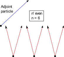
    Figure 3: Computation of P1โ€‹({kฮฝ})subscript๐‘ƒ1subscript๐‘˜๐œˆP_{1}(\{k_{\nu}\}): an example with n=6๐‘›6n=6. Red trajectories represent those particles whose quantum number must be equal to ฮป0=0subscript๐œ†00\lambda_{0}=0.
  • โ€ข

    Case 222 (nโ€ฒ=superscript๐‘›โ€ฒabsentn^{\prime}= even and n=๐‘›absentn= odd): also in this case the adjoint particle is created inbetween two different pairs, but when n๐‘›n is odd the result of equation (28) becomes:

    P2โ€‹({kฮฝ})=Pโ€‹(k1)โ€‹โ€ฆโ€‹Pโ€‹(kp+nโ€ฒ2)โ€‹P00โ€‹(kp+nโ€ฒ2+1)โ€‹โ€ฆโ€‹P00โ€‹(kp+nโ€ฒ2+nโˆ’12)โŸ|n|โˆ’12โ€‹timesร—โˆ‘ฮป=0,ยฑ1P0โ€‹ฮปโ€‹(kp+nโ€ฒ2+nโˆ’12+1)โ€‹Pโ€‹(kp+nโ€ฒ2+nโˆ’12+2)โ€‹โ€ฆโ€‹Pโ€‹(kM).subscript๐‘ƒ2subscript๐‘˜๐œˆ๐‘ƒsubscript๐‘˜1โ€ฆ๐‘ƒsubscript๐‘˜๐‘superscript๐‘›โ€ฒ2subscriptโŸsuperscript๐‘ƒ00subscript๐‘˜๐‘superscript๐‘›โ€ฒ21โ€ฆsuperscript๐‘ƒ00subscript๐‘˜๐‘superscript๐‘›โ€ฒ2๐‘›12๐‘›12timesmissing-subexpressionsubscript๐œ†0plus-or-minus1superscript๐‘ƒ0๐œ†subscript๐‘˜๐‘superscript๐‘›โ€ฒ2๐‘›121๐‘ƒsubscript๐‘˜๐‘superscript๐‘›โ€ฒ2๐‘›122โ€ฆ๐‘ƒsubscript๐‘˜๐‘€\begin{array}[]{lcl}P_{2}(\{k_{\nu}\})&=&P(k_{1})\dots P\left(k_{\frac{p+n^{\prime}}{2}}\right)\underbrace{P^{00}\left(k_{\frac{p+n^{\prime}}{2}+1}\right)\dots P^{00}\left(k_{\frac{p+n^{\prime}}{2}+\frac{n-1}{2}}\right)}_{\frac{|n|-1}{2}{\rm times}}\\ &\times&{\displaystyle\sum_{\lambda=0,\pm 1}}P^{0\lambda}\left(k_{\frac{p+n^{\prime}}{2}+\frac{n-1}{2}+1}\right)P\left(k_{\frac{p+n^{\prime}}{2}+\frac{n-1}{2}+2}\right)\dots P(k_{M}).\end{array} (30)

    In practice the last particle of the sequence of ฮปฮฝ=0subscript๐œ†๐œˆ0\lambda_{\nu}=0 belongs to a pair whose right-side partner can carry all possible quantum numbers.

  • โ€ข

    Case 333 (nโ€ฒ=superscript๐‘›โ€ฒabsentn^{\prime}= odd and n=๐‘›absentn= even): let us consider the case in which nโ€ฒsuperscript๐‘›โ€ฒn^{\prime} is an odd integer. In this case the adjoint particle is created within a quasiparticle pair, and the average over quantum numbers gives (nโ‰ 0๐‘›0n\neq 0):

    P3โ€‹({kฮฝ})=Pโ€‹(k1)โ€‹โ€ฆโ€‹Pโ€‹(kp+nโ€ฒโˆ’12)โ€‹โˆ‘ฮป=0,ยฑ1Pฮปโ€‹0โ€‹(kp+nโ€ฒโˆ’12+1)ร—P00โ€‹(kp+nโ€ฒโˆ’12+2)โ€‹โ€ฆโ€‹P00โ€‹(kp+nโ€ฒโˆ’12+n2)โŸ|n|2โˆ’1โ€‹tโ€‹iโ€‹mโ€‹eโ€‹sร—โˆ‘ฮป=0,ยฑ1P0โ€‹ฮปโ€‹(kp+nโ€ฒโˆ’12+n2+1)โ€‹Pโ€‹(kp+nโ€ฒโˆ’12+n2+2)โ€‹โ€ฆโ€‹Pโ€‹(kM).subscript๐‘ƒ3subscript๐‘˜๐œˆ๐‘ƒsubscript๐‘˜1โ€ฆ๐‘ƒsubscript๐‘˜๐‘superscript๐‘›โ€ฒ12subscript๐œ†0plus-or-minus1superscript๐‘ƒ๐œ†0subscript๐‘˜๐‘superscript๐‘›โ€ฒ121missing-subexpressionsubscriptโŸsuperscript๐‘ƒ00subscript๐‘˜๐‘superscript๐‘›โ€ฒ122โ€ฆsuperscript๐‘ƒ00subscript๐‘˜๐‘superscript๐‘›โ€ฒ12๐‘›2๐‘›21timesmissing-subexpressionsubscript๐œ†0plus-or-minus1superscript๐‘ƒ0๐œ†subscript๐‘˜๐‘superscript๐‘›โ€ฒ12๐‘›21๐‘ƒsubscript๐‘˜๐‘superscript๐‘›โ€ฒ12๐‘›22โ€ฆ๐‘ƒsubscript๐‘˜๐‘€\begin{array}[]{lcl}P_{3}(\{k_{\nu}\})&=&P(k_{1})\dots P\left(k_{\frac{p+n^{\prime}-1}{2}}\right){\displaystyle\sum_{\lambda=0,\pm 1}}P^{\lambda 0}\left(k_{\frac{p+n^{\prime}-1}{2}+1}\right)\\ &\times&\underbrace{P^{00}\left(k_{\frac{p+n^{\prime}-1}{2}+2}\right)\dots P^{00}\left(k_{\frac{p+n^{\prime}-1}{2}+\frac{n}{2}}\right)}_{\frac{|n|}{2}-1{\rm times}}\\ &\times&{\displaystyle\sum_{\lambda=0,\pm 1}}P^{0\lambda}\left(k_{\frac{p+n^{\prime}-1}{2}+\frac{n}{2}+1}\right)P\left(k_{\frac{p+n^{\prime}-1}{2}+\frac{n}{2}+2}\right)\dots P(k_{M}).\end{array} (31)

    The case n=0๐‘›0n=0 simply gives a sequence of M๐‘€M different Pโ€‹(kฮฝ)๐‘ƒsubscript๐‘˜๐œˆP(k_{\nu})โ€™s. When nโ€ฒsuperscript๐‘›โ€ฒn^{\prime} is odd and n๐‘›n even in the sequence of quantum numbers with ฮปฮฝ=0subscript๐œ†๐œˆ0\lambda_{\nu}=0 the first and the last one belong to pairs whose partner has no constraint on its quantum number ฮป๐œ†\lambda. This is the reason for the factors โˆ‘ฮป=0,ยฑ1P0โ€‹ฮปโ€‹(k)subscript๐œ†0plus-or-minus1superscript๐‘ƒ0๐œ†๐‘˜{\displaystyle\sum_{\lambda=0,\pm 1}}P^{0\lambda}(k) and โˆ‘ฮป=0,ยฑ1Pฮปโ€‹0โ€‹(k)subscript๐œ†0plus-or-minus1superscript๐‘ƒ๐œ†0๐‘˜{\displaystyle\sum_{\lambda=0,\pm 1}}P^{\lambda 0}(k) in the previous expression.

  • โ€ข

    Case 444 (nโ€ฒ=superscript๐‘›โ€ฒabsentn^{\prime}= odd and n=๐‘›absentn= odd): in this case the average over the set of quantum numbers gives:

    P4โ€‹({kฮฝ})=Pโ€‹(k1)โ€‹โ€ฆโ€‹Pโ€‹(kp+nโ€ฒโˆ’12)โ€‹โˆ‘ฮป=0,ยฑ1Pฮปโ€‹0โ€‹(kp+nโ€ฒโˆ’12+1)ร—P00โ€‹(kp+nโ€ฒโˆ’12+2)โ€‹โ€ฆโ€‹P00โ€‹(kp+nโ€ฒโˆ’12+nโˆ’12+1)โŸ|n|โˆ’12โ€‹timesร—Pโ€‹(kp+nโ€ฒโˆ’12+nโˆ’12+2)โ€‹โ€ฆโ€‹Pโ€‹(kM).subscript๐‘ƒ4subscript๐‘˜๐œˆ๐‘ƒsubscript๐‘˜1โ€ฆ๐‘ƒsubscript๐‘˜๐‘superscript๐‘›โ€ฒ12subscript๐œ†0plus-or-minus1superscript๐‘ƒ๐œ†0subscript๐‘˜๐‘superscript๐‘›โ€ฒ121missing-subexpressionsubscriptโŸsuperscript๐‘ƒ00subscript๐‘˜๐‘superscript๐‘›โ€ฒ122โ€ฆsuperscript๐‘ƒ00subscript๐‘˜๐‘superscript๐‘›โ€ฒ12๐‘›121๐‘›12timesmissing-subexpression๐‘ƒsubscript๐‘˜๐‘superscript๐‘›โ€ฒ12๐‘›122โ€ฆ๐‘ƒsubscript๐‘˜๐‘€\begin{array}[]{lcl}P_{4}(\{k_{\nu}\})&=&P(k_{1})\dots P\left(k_{\frac{p+n^{\prime}-1}{2}}\right){\displaystyle\sum_{\lambda=0,\pm 1}}P^{\lambda 0}\left(k_{\frac{p+n^{\prime}-1}{2}+1}\right)\\ &\times&\underbrace{P^{00}\left(k_{\frac{p+n^{\prime}-1}{2}+2}\right)\dots P^{00}\left(k_{\frac{p+n^{\prime}-1}{2}+\frac{n-1}{2}+1}\right)}_{\frac{|n|-1}{2}{\rm times}}\\ &\times&P\left(k_{\frac{p+n^{\prime}-1}{2}+\frac{n-1}{2}+2}\right)\dots P(k_{M}).\end{array} (32)

We are now ready to write down the global expression for the quantum number average:

โˆ‘ฮป1โ€ฒ,ฮป1โ€ฒโ€ฒโˆ‘ฮป2โ€ฒ,ฮป2โ€ฒโ€ฒโ€ฆโ€‹โˆ‘ฮปMโ€ฒ,ฮปMโ€ฒโ€ฒโˆฮฝ=1MPฮปฮฝโ€ฒโ€‹ฮปฮฝโ€ฒโ€ฒโ€‹(kฮฝ)โ€‹ฮด0,ฮปp+nโ€ฒ+1โ€‹ฮดฮปp+nโ€ฒ+1,ฮปp+nโ€ฒ+2โ€‹โ€ฆโ€‹ฮดฮปp+nโ€ฒ+nโˆ’1,ฮปp+nโ€ฒ+n=1+(โˆ’1)nโ€ฒ2โ€‹[1+(โˆ’1)n2โ€‹P1โ€‹({kฮฝ})+1โˆ’(โˆ’1)n2โ€‹P2โ€‹({kฮฝ})]+1โˆ’(โˆ’1)nโ€ฒ2โ€‹[1+(โˆ’1)n2โ€‹P3โ€‹({kฮฝ})+1โˆ’(โˆ’1)n2โ€‹P4โ€‹({kฮฝ})].subscriptsubscriptsuperscript๐œ†โ€ฒ1subscriptsuperscript๐œ†โ€ฒโ€ฒ1subscriptsubscriptsuperscript๐œ†โ€ฒ2subscriptsuperscript๐œ†โ€ฒโ€ฒ2โ€ฆsubscriptsubscriptsuperscript๐œ†โ€ฒ๐‘€subscriptsuperscript๐œ†โ€ฒโ€ฒ๐‘€superscriptsubscriptproduct๐œˆ1๐‘€superscript๐‘ƒsubscriptsuperscript๐œ†โ€ฒ๐œˆsubscriptsuperscript๐œ†โ€ฒโ€ฒ๐œˆsubscript๐‘˜๐œˆsubscript๐›ฟ0subscript๐œ†๐‘superscript๐‘›โ€ฒ1subscript๐›ฟsubscript๐œ†๐‘superscript๐‘›โ€ฒ1subscript๐œ†๐‘superscript๐‘›โ€ฒ2โ€ฆsubscript๐›ฟsubscript๐œ†๐‘superscript๐‘›โ€ฒ๐‘›1subscript๐œ†๐‘superscript๐‘›โ€ฒ๐‘›absent1superscript1superscript๐‘›โ€ฒ2delimited-[]1superscript1๐‘›2subscript๐‘ƒ1subscript๐‘˜๐œˆ1superscript1๐‘›2subscript๐‘ƒ2subscript๐‘˜๐œˆ1superscript1superscript๐‘›โ€ฒ2delimited-[]1superscript1๐‘›2subscript๐‘ƒ3subscript๐‘˜๐œˆ1superscript1๐‘›2subscript๐‘ƒ4subscript๐‘˜๐œˆ\begin{array}[]{l}{\displaystyle\sum_{\lambda^{\prime}_{1},\lambda^{\prime\prime}_{1}}\sum_{\lambda^{\prime}_{2},\lambda^{\prime\prime}_{2}}\dots\sum_{\lambda^{\prime}_{M},\lambda^{\prime\prime}_{M}}\prod_{\nu=1}^{M}}\,P^{\lambda^{\prime}_{\nu}\lambda^{\prime\prime}_{\nu}}(k_{\nu})\,\delta_{0,\lambda_{p+n^{\prime}+1}}\delta_{\lambda_{p+n^{\prime}+1},\lambda_{p+n^{\prime}+2}}\dots\delta_{\lambda_{p+n^{\prime}+n-1},\lambda_{p+n^{\prime}+n}}\\ ={\displaystyle\frac{1+(-1)^{n^{\prime}}}{2}}\left[{\displaystyle\frac{1+(-1)^{n}}{2}}P_{1}(\{k_{\nu}\})+{\displaystyle\frac{1-(-1)^{n}}{2}}P_{2}(\{k_{\nu}\})\right]\\ +{\displaystyle\frac{1-(-1)^{n^{\prime}}}{2}}\left[{\displaystyle\frac{1+(-1)^{n}}{2}}P_{3}(\{k_{\nu}\})+{\displaystyle\frac{1-(-1)^{n}}{2}}P_{4}(\{k_{\nu}\})\right].\end{array} (33)

This expression is a function of (n,nโ€ฒ)๐‘›superscript๐‘›โ€ฒ(n,n^{\prime}) and the set of quantum momenta of a particular quasiparticle configuration. It is worth noticing that n๐‘›n and nโ€ฒsuperscript๐‘›โ€ฒn^{\prime} enter the expression for Pisubscript๐‘ƒ๐‘–P_{i}, i=1,โ€ฆ,4๐‘–1โ€ฆ4i=1,\dots,4 in different ways. While n๐‘›n tells us how long the sequence is, nโ€ฒsuperscript๐‘›โ€ฒn^{\prime} gives us information about the starting point of the sequence and can easily be absorbed into the definition of p๐‘p. As we shall see, for the actual computation of the relaxation function R๐‘…R the starting position of the sequence is not important, what matters is only the length of the sequence itself.
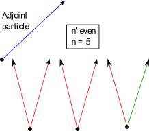
Refer to caption
Figure 4: Computation of P2โ€‹({kฮฝ})subscript๐‘ƒ2subscript๐‘˜๐œˆP_{2}(\{k_{\nu}\}): an example with n=5๐‘›5n=5.

4.2 The semi-classical average in action

We must now compute the average of the previous quantity over all possible initial positions and momenta. Namely we must take the following average:

โˆซโˆ’L/2L/2dโ€‹x1Lโ€‹โ€ฆโ€‹dโ€‹xMLโ€‹โˆ‘k1>0โ€ฆโ€‹โˆ‘kM>0โˆ‘n=โˆ’โˆž+โˆž(โˆ’1)nโ€‹ฮดn,โˆ‘ฮฝ2โ€‹[โ€ฆ]โ€‹โˆ‘nโ€ฒ=โˆ’โˆž+โˆžฮดnโ€ฒ,โˆ‘ฮฝ1โ€‹[โ€ฆ],superscriptsubscript๐ฟ2๐ฟ2๐‘‘subscript๐‘ฅ1๐ฟโ€ฆ๐‘‘subscript๐‘ฅ๐‘€๐ฟsubscriptsubscript๐‘˜10โ€ฆsubscriptsubscript๐‘˜๐‘€0superscriptsubscript๐‘›superscript1๐‘›subscript๐›ฟ๐‘›subscriptsubscript๐œˆ2delimited-[]โ€ฆsuperscriptsubscriptsuperscript๐‘›โ€ฒsubscript๐›ฟsuperscript๐‘›โ€ฒsubscriptsubscript๐œˆ1delimited-[]โ€ฆ\qquad{\displaystyle\int_{-L/2}^{L/2}\frac{dx_{1}}{L}\dots\frac{dx_{M}}{L}\sum_{k_{1}>0}\dots\sum_{k_{M}>0}}\,\,{\displaystyle\sum_{n=-\infty}^{+\infty}}(-1)^{n}\delta_{n,\sum_{\nu_{2}}}\left[\dots\right]{\displaystyle\sum_{n^{\prime}=-\infty}^{+\infty}}\delta_{n^{\prime},\sum_{\nu_{1}}}\left[\dots\right], (34)

where the quantity in the square brackets is given by equation (33). We can split this average into four pieces, let us call them A,B,C๐ด๐ต๐ถA,B,C and D๐ทD, one for each Piโ€‹({kฮฝ})subscript๐‘ƒ๐‘–subscript๐‘˜๐œˆP_{i}(\{k_{\nu}\}) respectively, where i=1,โ€ฆ,4๐‘–1โ€ฆ4i=1,\dots,4. We shall do the computation of the term which contains P1โ€‹({kฮฝ})subscript๐‘ƒ1subscript๐‘˜๐œˆP_{1}(\{k_{\nu}\}) in some detail; the other cases are straightforward modifications.
Let us compute explicity A๐ดA, the first addend of the right side of equation (33), where the first summation over nโ€ฒsuperscript๐‘›โ€ฒn^{\prime} gets immediately canceled out by the corresponding Kronecker delta because nโ€ฒsuperscript๐‘›โ€ฒn^{\prime} itself enters the function P1โ€‹({kฮฝ})subscript๐‘ƒ1subscript๐‘˜๐œˆP_{1}(\{k_{\nu}\}) trivially, therefore we have:

A=โˆซโˆ’L/2L/2dโ€‹x1Lโ€‹โ€ฆโ€‹dโ€‹xMLโ€‹โˆ‘k1>0โ€ฆโ€‹โˆ‘kM>0โˆ‘n=โˆ’โˆž+โˆž(โˆ’1)nโ€‹ฮดn,โˆ‘ฮฝ2โ€‹[โ€ฆ]ร—(1+(โˆ’1)โˆ‘ฮฝ1[โ€ฆ]2โ€‹1+(โˆ’1)n2โ€‹P1โ€‹({kฮฝ})),๐ดsuperscriptsubscript๐ฟ2๐ฟ2๐‘‘subscript๐‘ฅ1๐ฟโ€ฆ๐‘‘subscript๐‘ฅ๐‘€๐ฟsubscriptsubscript๐‘˜10โ€ฆsubscriptsubscript๐‘˜๐‘€0superscriptsubscript๐‘›superscript1๐‘›subscript๐›ฟ๐‘›subscriptsubscript๐œˆ2delimited-[]โ€ฆmissing-subexpressionmissing-subexpressionabsent1superscript1subscriptsubscript๐œˆ1delimited-[]โ€ฆ21superscript1๐‘›2subscript๐‘ƒ1subscript๐‘˜๐œˆ\begin{array}[]{lcl}A&=&{\displaystyle\int_{-L/2}^{L/2}\frac{dx_{1}}{L}\dots\frac{dx_{M}}{L}\sum_{k_{1}>0}\dots\sum_{k_{M}>0}}\,\,{\displaystyle\sum_{n=-\infty}^{+\infty}}(-1)^{n}\delta_{n,\sum_{\nu_{2}}}\left[\dots\right]\\ &&\times\left({\displaystyle\frac{1+(-1)^{\sum_{\nu_{1}}[\dots]}}{2}}{\displaystyle\frac{1+(-1)^{n}}{2}}P_{1}(\{k_{\nu}\})\right),\end{array} (35)
Refer to caption
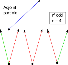
Figure 5: Computation of P3โ€‹({kฮฝ})subscript๐‘ƒ3subscript๐‘˜๐œˆP_{3}(\{k_{\nu}\}): an example with nโ€ฒsuperscript๐‘›โ€ฒn^{\prime} odd and n=4๐‘›4n=4.

where โˆ‘ฮฝ1[โ€ฆ]subscriptsubscript๐œˆ1delimited-[]โ€ฆ\sum_{\nu_{1}}[\dots] is specified by (19). A๐ดA can itself be splitted into two pieces, say A1subscript๐ด1A_{1} and A2subscript๐ด2A_{2}, with A=A1+A2๐ดsubscript๐ด1subscript๐ด2A=A_{1}+A_{2} which correspond to the two contributions to the integration of the terms into the bracket, namely:

A1=โˆซโˆ’L/2L/2dโ€‹x1Lโ€‹โ€ฆโ€‹dโ€‹xMLโ€‹โˆ‘k1>0โ€ฆโ€‹โˆ‘kM>0โˆ‘n=โˆ’โˆž+โˆž(โˆ’1)nโ€‹ฮดn,โˆ‘ฮฝ2โ€‹[โ€ฆ]ร—(1+(โˆ’1)n4โ€‹P1โ€‹({kฮฝ})),subscript๐ด1superscriptsubscript๐ฟ2๐ฟ2๐‘‘subscript๐‘ฅ1๐ฟโ€ฆ๐‘‘subscript๐‘ฅ๐‘€๐ฟsubscriptsubscript๐‘˜10โ€ฆsubscriptsubscript๐‘˜๐‘€0superscriptsubscript๐‘›superscript1๐‘›subscript๐›ฟ๐‘›subscriptsubscript๐œˆ2delimited-[]โ€ฆmissing-subexpressionmissing-subexpressionabsent1superscript1๐‘›4subscript๐‘ƒ1subscript๐‘˜๐œˆ\begin{array}[]{lcl}A_{1}&=&{\displaystyle\int_{-L/2}^{L/2}\frac{dx_{1}}{L}\dots\frac{dx_{M}}{L}\sum_{k_{1}>0}\dots\sum_{k_{M}>0}}\,\,{\displaystyle\sum_{n=-\infty}^{+\infty}}(-1)^{n}\delta_{n,\sum_{\nu_{2}}}\left[\dots\right]\\ &&\times\left({\displaystyle\frac{1+(-1)^{n}}{4}}P_{1}(\{k_{\nu}\})\right),\end{array} (36)

and

A2=โˆซโˆ’L/2L/2dโ€‹x1Lโ€‹โ€ฆโ€‹dโ€‹xMLโ€‹โˆ‘k1>0โ€ฆโ€‹โˆ‘kM>0โˆ‘n=โˆ’โˆž+โˆž(โˆ’1)nโ€‹ฮดn,โˆ‘ฮฝ2โ€‹[โ€ฆ]ร—((โˆ’1)โˆ‘ฮฝ1[โ€ฆ]2โ€‹1+(โˆ’1)n2โ€‹P1โ€‹({kฮฝ})).subscript๐ด2superscriptsubscript๐ฟ2๐ฟ2๐‘‘subscript๐‘ฅ1๐ฟโ€ฆ๐‘‘subscript๐‘ฅ๐‘€๐ฟsubscriptsubscript๐‘˜10โ€ฆsubscriptsubscript๐‘˜๐‘€0superscriptsubscript๐‘›superscript1๐‘›subscript๐›ฟ๐‘›subscriptsubscript๐œˆ2delimited-[]โ€ฆmissing-subexpressionmissing-subexpressionabsentsuperscript1subscriptsubscript๐œˆ1delimited-[]โ€ฆ21superscript1๐‘›2subscript๐‘ƒ1subscript๐‘˜๐œˆ\begin{array}[]{lcl}A_{2}&=&{\displaystyle\int_{-L/2}^{L/2}\frac{dx_{1}}{L}\dots\frac{dx_{M}}{L}\sum_{k_{1}>0}\dots\sum_{k_{M}>0}}\,\,{\displaystyle\sum_{n=-\infty}^{+\infty}}(-1)^{n}\delta_{n,\sum_{\nu_{2}}}\left[\dots\right]\\ &&\times\left({\displaystyle\frac{(-1)^{\sum_{\nu_{1}}[\dots]}}{2}}{\displaystyle\frac{1+(-1)^{n}}{2}}P_{1}(\{k_{\nu}\})\right).\end{array} (37)

Let us start by computing the contribution of A1subscript๐ด1A_{1}. By making use of the following integral representation of the Kronecker delta

ฮดn,โˆ‘ฮฝ[โ€ฆ]=12โ€‹ฯ€โ€‹โˆซโˆ’ฯ€ฯ€๐‘‘ฯ•โ€‹eiโ€‹ฯ•โ€‹(nโˆ’โˆ‘ฮฝ[โ€ฆ]),subscript๐›ฟ๐‘›subscript๐œˆdelimited-[]โ€ฆ12๐œ‹superscriptsubscript๐œ‹๐œ‹differential-ditalic-ฯ•superscripte๐‘–italic-ฯ•๐‘›subscript๐œˆdelimited-[]โ€ฆ\delta_{n,\sum_{\nu}[\dots]}=\frac{1}{2\pi}{\displaystyle\int_{-\pi}^{\pi}}d\phi\,{\rm e}^{i\phi(n-\sum_{\nu}[\dots])}, (38)

we can write A1subscript๐ด1A_{1} as:

โˆซโˆ’ฯ€ฯ€dโ€‹ฯ•2โ€‹ฯ€โ€‹โˆ‘n=โˆ’โˆž+โˆž(โˆ’1)nโ€‹eiโ€‹nโ€‹ฯ•โ€‹1+(โˆ’1)n2โ€‹โˆ‘k1>0โ€ฆโ€‹โˆ‘kM>0โˆซโˆ’L/2L/2dโ€‹x1Lโ€‹โ€ฆโ€‹dโ€‹xMLโ€‹eโˆ’iโ€‹ฯ•โ€‹โˆ‘ฮฝ2[โ€ฆ]โ€‹P1โ€‹({kฮฝ})2.superscriptsubscript๐œ‹๐œ‹๐‘‘italic-ฯ•2๐œ‹superscriptsubscript๐‘›superscript1๐‘›superscripte๐‘–๐‘›italic-ฯ•1superscript1๐‘›2subscriptsubscript๐‘˜10โ€ฆsubscriptsubscript๐‘˜๐‘€0superscriptsubscript๐ฟ2๐ฟ2๐‘‘subscript๐‘ฅ1๐ฟโ€ฆ๐‘‘subscript๐‘ฅ๐‘€๐ฟsuperscripte๐‘–italic-ฯ•subscriptsubscript๐œˆ2delimited-[]โ€ฆsubscript๐‘ƒ1subscript๐‘˜๐œˆ2\quad\int_{-\pi}^{\pi}\frac{d\phi}{2\pi}{\displaystyle\sum_{n=-\infty}^{+\infty}}(-1)^{n}{\rm e}^{in\phi}{\displaystyle\frac{1+(-1)^{n}}{2}}{\displaystyle\sum_{k_{1}>0}\dots\sum_{k_{M}>0}}\,\,{\displaystyle\int_{-L/2}^{L/2}\frac{dx_{1}}{L}\dots\frac{dx_{M}}{L}}\,{\rm e}^{-i\phi\sum_{\nu_{2}}[\dots]}\,\frac{P_{1}(\{k_{\nu}\})}{2}. (39)

Now we first compute the spatial integration in equation 39, then the integral over the momenta and finally the sum over n๐‘›n.

Refer to caption
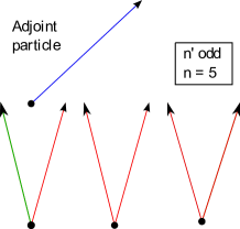
Figure 6: Computation of P4โ€‹({kฮฝ})subscript๐‘ƒ4subscript๐‘˜๐œˆP_{4}(\{k_{\nu}\}): an example with nโ€ฒsuperscript๐‘›โ€ฒn^{\prime} odd and n=5๐‘›5n=5.

The spatial integration.

Now we want to compute the spatial integral, remembering that the sum โˆ‘ฮฝ2[โ€ฆ]subscriptsubscript๐œˆ2delimited-[]โ€ฆ\sum_{\nu_{2}}[\dots] is specified in equation (21). We begin by considering x>0๐‘ฅ0x>0, t2>t1subscript๐‘ก2subscript๐‘ก1t_{2}>t_{1} and x<vmโ€‹aโ€‹xโ€‹(t2โˆ’t1)๐‘ฅsubscript๐‘ฃ๐‘š๐‘Ž๐‘ฅsubscript๐‘ก2subscript๐‘ก1x<v_{max}(t_{2}-t_{1}), where vmโ€‹aโ€‹xsubscript๐‘ฃ๐‘š๐‘Ž๐‘ฅv_{max} is the maximal velocity of the excitations of the model (in the appendix B we will show the general result for arbitrary times and distances). We will refer to this situation as the within-the-light-cone case. The spatial integral factorizes in a straightforward way, thus we can write:

โˆซโˆ’L/2L/2dโ€‹x1Lโ€ฆdโ€‹xMLeโˆ’iโ€‹ฯ•โ€‹โˆ‘ฮฝ2[โ€ฆ]=โˆฮฝ=1M{1โˆ’2โ€‹vkฮฝโ€‹tL(1โˆ’cosฯ•)ฮ˜[vkฮฝtโˆ’x]โˆ’2โ€‹iโ€‹xโ€‹sinโกฯ•Lโ€‹ฮ˜โ€‹[vkฮฝโ€‹tโˆ’x]โˆ’2โ€‹xLโ€‹(iโ€‹sinโกฯ•+2โ€‹sin2โก(ฯ•/2))โ€‹ฮ˜โ€‹[xโˆ’vkฮฝโ€‹t]โ€‹ฮ˜โ€‹[vkฮฝโ€‹Tโˆ’x]โˆ’(vkฮฝโ€‹TL(1+cos(2ฯ•)โˆ’isin(2ฯ•)โˆ’cosฯ•+isinฯ•)+xL(isin(2ฯ•)+2sin2ฯ•))ฮ˜[xโˆ’vkฮฝT]},\begin{array}[]{l}\quad{\displaystyle\int_{-L/2}^{L/2}\frac{dx_{1}}{L}\dots\frac{dx_{M}}{L}}\,{\rm e}^{-i\phi\sum_{\nu_{2}}[\dots]}={\displaystyle\prod_{\nu=1}^{M}}\left\{1-\frac{2v_{k_{\nu}}t}{L}(1-\cos\phi)\Theta[v_{k_{\nu}}t-x]\right.\\ \\ \quad\left.-\frac{2ix\sin\phi}{L}\Theta[v_{k_{\nu}}t-x]-\frac{2x}{L}\left(i\sin\phi+2\sin^{2}(\phi/2)\right)\Theta[x-v_{k_{\nu}}t]\Theta[v_{k_{\nu}}T-x]\right.\\ \\ \quad-\left.\left(\frac{v_{k_{\nu}}T}{L}(1+\cos(2\phi)-i\sin(2\phi)-\cos\phi+i\sin\phi)+\frac{x}{L}(i\sin(2\phi)+2\sin^{2}\phi)\right)\Theta[x-v_{k_{\nu}}T]\right\},\end{array} (40)

where vkฮฝsubscript๐‘ฃsubscript๐‘˜๐œˆv_{k_{\nu}} is the particle velocity defined by vkโ‰กโˆ‚ฯตโ€‹(k)โˆ‚ksubscript๐‘ฃ๐‘˜italic-ฯต๐‘˜๐‘˜v_{k}\equiv\frac{\partial\epsilon(k)}{\partial k}, tโ‰กt2โˆ’t1๐‘กsubscript๐‘ก2subscript๐‘ก1t\equiv t_{2}-t_{1} and Tโ‰กt2+t1๐‘‡subscript๐‘ก2subscript๐‘ก1T\equiv t_{2}+t_{1}. Let us notice the following definition of the probability Pโ€‹(k)๐‘ƒ๐‘˜P(k):

Pโ€‹(k)โ‰กfkM,M=โˆ‘k>0fk,formulae-sequence๐‘ƒ๐‘˜subscript๐‘“๐‘˜๐‘€๐‘€subscript๐‘˜0subscript๐‘“๐‘˜P(k)\equiv{\displaystyle\frac{f_{k}}{M}},\qquad M=\sum_{k>0}f_{k}, (41)

where fksubscript๐‘“๐‘˜f_{k} is the occupation number of the k๐‘˜k-mode. Furthermore, the following identities can be useful in taking the thermodynamic limit:

โˆ‘k>0Pโ€‹(k)โ€‹vkLโ‰กโˆ‘k>0fkโ€‹vkLโ€‹โˆ‘k>0fkโŸถโˆซ0โˆždโ€‹k2โ€‹ฯ€โ€‹fkโ€‹vkM,โˆ‘k>0Pโ€‹(k)Lโ‰กโˆ‘k>0fkLโ€‹โˆ‘k>0fkโŸถโˆซ0โˆždโ€‹k2โ€‹ฯ€โ€‹fkM.formulae-sequencesubscript๐‘˜0๐‘ƒ๐‘˜subscript๐‘ฃ๐‘˜๐ฟsubscript๐‘˜0subscript๐‘“๐‘˜subscript๐‘ฃ๐‘˜๐ฟsubscript๐‘˜0subscript๐‘“๐‘˜โŸถsuperscriptsubscript0๐‘‘๐‘˜2๐œ‹subscript๐‘“๐‘˜subscript๐‘ฃ๐‘˜๐‘€subscript๐‘˜0๐‘ƒ๐‘˜๐ฟsubscript๐‘˜0subscript๐‘“๐‘˜๐ฟsubscript๐‘˜0subscript๐‘“๐‘˜โŸถsuperscriptsubscript0๐‘‘๐‘˜2๐œ‹subscript๐‘“๐‘˜๐‘€\quad{\displaystyle\frac{{\displaystyle\sum_{k>0}P(k)v_{k}}}{L}}\equiv{\displaystyle\frac{{\displaystyle\sum_{k>0}f_{k}v_{k}}}{L{\displaystyle\sum_{k>0}f_{k}}}}\longrightarrow{\displaystyle\frac{{\displaystyle\int_{0}^{\infty}\frac{dk}{2\pi}f_{k}v_{k}}}{M}},\qquad\qquad{\displaystyle\frac{{\displaystyle\sum_{k>0}P(k)}}{L}}\equiv{\displaystyle\frac{{\displaystyle\sum_{k>0}f_{k}}}{L{\displaystyle\sum_{k>0}f_{k}}}}\longrightarrow{\displaystyle\frac{{\displaystyle\int_{0}^{\infty}\frac{dk}{2\pi}f_{k}}}{M}}. (42)

Integration over the momenta.

Let us now compute the average over the momenta of the previous result, taking the limit L,Mโ†’โˆžโ†’๐ฟ๐‘€L,M\to\infty (M/Lโ‰กฯ๐‘€๐ฟ๐œŒM/L\equiv\rho fixed). The basic idea behind this limit is that we can replace M๐‘€M by the average particle number, Mโ†’ฯโ€‹Lโ†’๐‘€๐œŒ๐ฟM\to\rho L without changing the final result. Namely we have:

limM,Lโ†’โˆžโˆ‘k1>0โ€ฆโ€‹โˆ‘kM>0P1โ€‹({kฮฝ})โ€‹โˆฮฝ=1M{โ€ฆ},subscriptโ†’๐‘€๐ฟsubscriptsubscript๐‘˜10โ€ฆsubscriptsubscript๐‘˜๐‘€0subscript๐‘ƒ1subscript๐‘˜๐œˆsuperscriptsubscriptproduct๐œˆ1๐‘€โ€ฆ{\displaystyle\lim_{M,L\to\infty}}{\displaystyle\sum_{k_{1}>0}\dots\sum_{k_{M}>0}}P_{1}(\{k_{\nu}\}){\displaystyle\prod_{\nu=1}^{M}}\left\{\dots\right\}, (43)

where P1โ€‹({kฮฝ})subscript๐‘ƒ1subscript๐‘˜๐œˆP_{1}(\{k_{\nu}\}) is given by (29) and the {โ€ฆ}โ€ฆ\{\dots\} are the right-hand terms of equation (40). This expression can be simply evaluated to yield:

limM,Lโ†’โˆžโˆ‘{kฮฝ>0}P1โ€‹({kฮฝ})โ€‹โˆฮฝ=1M(โ€ฆ)=expโก{โˆ’tโ€‹(1โˆ’cosโกฯ•)โ€‹โˆซ0โˆždโ€‹kฯ€โ€‹fkโ€‹vkโ€‹ฮ˜โ€‹[vkโ€‹tโˆ’x]โˆ’2โ€‹xโ€‹sin2โก(ฯ•/2)โ€‹โˆซ0โˆždโ€‹kฯ€โ€‹fkโ€‹ฮ˜โ€‹[xโˆ’vkโ€‹t]โ€‹ฮ˜โ€‹[vkโ€‹Tโˆ’x]}ร—expโก{โˆ’Tโ€‹(1+cosโก(2โ€‹ฯ•)โˆ’iโ€‹sinโก(2โ€‹ฯ•)โˆ’2โ€‹cosโกฯ•+2โ€‹iโ€‹sinโกฯ•)โ€‹โˆซ0โˆždโ€‹k2โ€‹ฯ€โ€‹fkโ€‹ฮ˜โ€‹[xโˆ’vkโ€‹T]}ร—expโก{โˆ’iโ€‹xโ€‹sinโกฯ•โ€‹โˆซ0โˆždโ€‹kฯ€โ€‹fkโ€‹(ฮ˜โ€‹[vkโ€‹tโˆ’x]+ฮ˜โ€‹[xโˆ’vkโ€‹t]โ€‹ฮ˜โ€‹[vkโ€‹Tโˆ’x])}ร—expโก{โˆ’xโ€‹(2โ€‹sin2โกฯ•+iโ€‹sinโก(2โ€‹ฯ•))โ€‹โˆซ0โˆždโ€‹k2โ€‹ฯ€โ€‹fkโ€‹ฮ˜โ€‹[xโˆ’vkโ€‹T]}โ€‹(P00)|n|/2,subscriptโ†’๐‘€๐ฟsubscriptsubscript๐‘˜๐œˆ0subscript๐‘ƒ1subscript๐‘˜๐œˆsuperscriptsubscriptproduct๐œˆ1๐‘€โ€ฆabsent๐‘ก1italic-ฯ•superscriptsubscript0๐‘‘๐‘˜๐œ‹subscript๐‘“๐‘˜subscript๐‘ฃ๐‘˜ฮ˜delimited-[]subscript๐‘ฃ๐‘˜๐‘ก๐‘ฅ2๐‘ฅsuperscript2italic-ฯ•2superscriptsubscript0๐‘‘๐‘˜๐œ‹subscript๐‘“๐‘˜ฮ˜delimited-[]๐‘ฅsubscript๐‘ฃ๐‘˜๐‘กฮ˜delimited-[]subscript๐‘ฃ๐‘˜๐‘‡๐‘ฅabsent๐‘‡12italic-ฯ•๐‘–2italic-ฯ•2italic-ฯ•2๐‘–italic-ฯ•superscriptsubscript0๐‘‘๐‘˜2๐œ‹subscript๐‘“๐‘˜ฮ˜delimited-[]๐‘ฅsubscript๐‘ฃ๐‘˜๐‘‡absent๐‘–๐‘ฅitalic-ฯ•superscriptsubscript0๐‘‘๐‘˜๐œ‹subscript๐‘“๐‘˜ฮ˜delimited-[]subscript๐‘ฃ๐‘˜๐‘ก๐‘ฅฮ˜delimited-[]๐‘ฅsubscript๐‘ฃ๐‘˜๐‘กฮ˜delimited-[]subscript๐‘ฃ๐‘˜๐‘‡๐‘ฅabsent๐‘ฅ2superscript2italic-ฯ•๐‘–2italic-ฯ•superscriptsubscript0๐‘‘๐‘˜2๐œ‹subscript๐‘“๐‘˜ฮ˜delimited-[]๐‘ฅsubscript๐‘ฃ๐‘˜๐‘‡superscriptsuperscript๐‘ƒ00๐‘›2\begin{array}[]{l}{\displaystyle\lim_{M,L\to\infty}}\,{\displaystyle\sum_{\{k_{\nu}>0\}}P_{1}(\{k_{\nu}\})}{\displaystyle\prod_{\nu=1}^{M}}\left(\dots\right)\\ =\exp{\left\{-t(1-\cos\phi){\displaystyle\int_{0}^{\infty}\frac{dk}{\pi}f_{k}\,v_{k}}\Theta[v_{k}t-x]-2x\sin^{2}(\phi/2){\displaystyle\int_{0}^{\infty}\frac{dk}{\pi}f_{k}}\,\Theta[x-v_{k}t]\Theta[v_{k}T-x]\right\}}\\ \quad\times\exp{\left\{-T(1+\cos(2\phi)-i\sin(2\phi)-2\cos\phi+2i\sin\phi){\displaystyle\int_{0}^{\infty}\frac{dk}{2\pi}f_{k}}\,\Theta[x-v_{k}T]\right\}}\\ \quad\times\exp{\left\{-ix\sin\phi{\displaystyle\int_{0}^{\infty}\frac{dk}{\pi}f_{k}}\,(\Theta[v_{k}t-x]+\Theta[x-v_{k}t]\Theta[v_{k}T-x])\right\}}\\ \quad\times\exp{\left\{-x(2\sin^{2}\phi+i\sin(2\phi)){\displaystyle\int_{0}^{\infty}\frac{dk}{2\pi}f_{k}}\,\Theta[x-v_{k}T]\right\}}(P^{00})^{|n|/2},\\ \\ \end{array} (44)

where P00=โˆซ0โˆždโ€‹k2โ€‹ฯ€โ€‹P00โ€‹(k)superscript๐‘ƒ00superscriptsubscript0๐‘‘๐‘˜2๐œ‹superscript๐‘ƒ00๐‘˜P^{00}=\int_{0}^{\infty}\frac{dk}{2\pi}P^{00}(k) and P00โ€‹(k)superscript๐‘ƒ00๐‘˜P^{00}(k) is now a probability density. We can now take the limit when T๐‘‡T is very large (x/Tโ‰ชvmโ€‹aโ€‹xmuch-less-than๐‘ฅ๐‘‡subscript๐‘ฃ๐‘š๐‘Ž๐‘ฅx/T\ll v_{max}), assuming that Tโ€‹โˆซ0โˆždโ€‹k2โ€‹ฯ€โ€‹fkโ€‹vkโ€‹ฮ˜โ€‹[xโˆ’vkโ€‹T]โ†’0โ†’๐‘‡superscriptsubscript0๐‘‘๐‘˜2๐œ‹subscript๐‘“๐‘˜subscript๐‘ฃ๐‘˜ฮ˜delimited-[]๐‘ฅsubscript๐‘ฃ๐‘˜๐‘‡0T\int_{0}^{\infty}\frac{dk}{2\pi}f_{k}v_{k}\,\Theta[x-v_{k}T]\to 0, so the previous expression simplifies, giving:

โ€ฆ=expโก{โˆ’tโ€‹(1โˆ’cosโกฯ•)โ€‹โˆซ0โˆždโ€‹kฯ€โ€‹fkโ€‹vkโ€‹ฮ˜โ€‹[vkโ€‹tโˆ’x]โˆ’2โ€‹xโ€‹sin2โก(ฯ•/2)โ€‹โˆซ0โˆždโ€‹kฯ€โ€‹fkโ€‹ฮ˜โ€‹[xโˆ’vkโ€‹t]}ร—expโก{โˆ’iโ€‹xโ€‹sinโกฯ•โ€‹โˆซ0โˆždโ€‹kฯ€โ€‹fk}โ€‹(P00)|n|/2.โ€ฆ๐‘ก1italic-ฯ•superscriptsubscript0๐‘‘๐‘˜๐œ‹subscript๐‘“๐‘˜subscript๐‘ฃ๐‘˜ฮ˜delimited-[]subscript๐‘ฃ๐‘˜๐‘ก๐‘ฅ2๐‘ฅsuperscript2italic-ฯ•2superscriptsubscript0๐‘‘๐‘˜๐œ‹subscript๐‘“๐‘˜ฮ˜delimited-[]๐‘ฅsubscript๐‘ฃ๐‘˜๐‘กmissing-subexpression๐‘–๐‘ฅitalic-ฯ•superscriptsubscript0๐‘‘๐‘˜๐œ‹subscript๐‘“๐‘˜superscriptsuperscript๐‘ƒ00๐‘›2\begin{array}[]{lcl}\dots&=&\exp{\left\{-t(1-\cos\phi){\displaystyle\int_{0}^{\infty}\frac{dk}{\pi}f_{k}\,v_{k}}\Theta[v_{k}t-x]-2x\sin^{2}(\phi/2){\displaystyle\int_{0}^{\infty}\frac{dk}{\pi}f_{k}}\,\Theta[x-v_{k}t]\right\}}\\ &\times&\exp{\left\{-ix\sin\phi{\displaystyle\int_{0}^{\infty}\frac{dk}{\pi}f_{k}}\right\}}\,(P^{00})^{|n|/2}.\end{array} (45)

Before computing the sum over n๐‘›n it is convenient to obtain the analogy of equation (45) for the case A2subscript๐ด2A_{2}, and see which contributions survive in the limit of T๐‘‡T very large . For A2subscript๐ด2A_{2} we start with:

โˆ‘k1>0โ€ฆโ€‹โˆ‘kM>0โˆซโˆ’L/2L/2dโ€‹x1Lโ€‹โ€ฆโ€‹dโ€‹xMLโ€‹eโˆ’iโ€‹ฯ•โ€‹โˆ‘ฮฝ2[โ€ฆ]โ€‹P1โ€‹({kฮฝ})โ€‹(โˆ’1)โˆ‘ฮฝ1[โ€ฆ],subscriptsubscript๐‘˜10โ€ฆsubscriptsubscript๐‘˜๐‘€0superscriptsubscript๐ฟ2๐ฟ2๐‘‘subscript๐‘ฅ1๐ฟโ€ฆ๐‘‘subscript๐‘ฅ๐‘€๐ฟsuperscripte๐‘–italic-ฯ•subscriptsubscript๐œˆ2delimited-[]โ€ฆsubscript๐‘ƒ1subscript๐‘˜๐œˆsuperscript1subscriptsubscript๐œˆ1delimited-[]โ€ฆ{\displaystyle\sum_{k_{1}>0}\dots\sum_{k_{M}>0}}\,{\displaystyle\int_{-L/2}^{L/2}\frac{dx_{1}}{L}\dots\frac{dx_{M}}{L}}\,{\rm e}^{-i\phi\sum_{\nu_{2}}[\dots]}\,P_{1}(\{k_{\nu}\})\,(-1)^{\sum_{\nu_{1}}[\dots]}, (46)

then by repeating the same steps we end up with:

limMโ†’โˆžโˆ‘k1>0โ€ฆโ€‹โˆ‘kM>0P1โ€‹({kฮฝ})โ€‹โˆฮฝ=1M(โ€ฆ)=expโก(โˆ’(Tโˆ’tโ€‹cosโกฯ•)โ€‹โˆซ0โˆždโ€‹k2โ€‹ฯ€โ€‹fkโ€‹vkโˆ’iโ€‹xโ€‹sinโกฯ•โ€‹โˆซ0โˆždโ€‹k2โ€‹ฯ€โ€‹fkโ€‹ฮ˜โ€‹[vkโ€‹tโˆ’x])ร—expโก(โˆ’iโ€‹tโ€‹sinโกฯ•โ€‹โˆซ0โˆždโ€‹k2โ€‹ฯ€โ€‹fkโ€‹vkโ€‹ฮ˜โ€‹[xโˆ’vkโ€‹t])โ€‹(P00)|n|/2.subscriptโ†’๐‘€subscriptsubscript๐‘˜10โ€ฆsubscriptsubscript๐‘˜๐‘€0subscript๐‘ƒ1subscript๐‘˜๐œˆsuperscriptsubscriptproduct๐œˆ1๐‘€โ€ฆabsent๐‘‡๐‘กitalic-ฯ•superscriptsubscript0๐‘‘๐‘˜2๐œ‹subscript๐‘“๐‘˜subscript๐‘ฃ๐‘˜๐‘–๐‘ฅitalic-ฯ•superscriptsubscript0๐‘‘๐‘˜2๐œ‹subscript๐‘“๐‘˜ฮ˜delimited-[]subscript๐‘ฃ๐‘˜๐‘ก๐‘ฅabsent๐‘–๐‘กitalic-ฯ•superscriptsubscript0๐‘‘๐‘˜2๐œ‹subscript๐‘“๐‘˜subscript๐‘ฃ๐‘˜ฮ˜delimited-[]๐‘ฅsubscript๐‘ฃ๐‘˜๐‘กsuperscriptsuperscript๐‘ƒ00๐‘›2\begin{array}[]{l}{\displaystyle\lim_{M\to\infty}}\,{\displaystyle\sum_{k_{1}>0}\dots\sum_{k_{M}>0}}P_{1}(\{k_{\nu}\}){\displaystyle\prod_{\nu=1}^{M}}\left(\dots\right)\\ =\exp{\left(-(T-t\cos\phi){\displaystyle\int_{0}^{\infty}\frac{dk}{2\pi}f_{k}v_{k}}-ix\sin\phi{\displaystyle\int_{0}^{\infty}\frac{dk}{2\pi}f_{k}\,\Theta[v_{k}t-x]}\right)}\\ \times\exp{\left(-it\sin\phi{\displaystyle\int_{0}^{\infty}\frac{dk}{2\pi}f_{k}v_{k}\,\Theta[x-v_{k}t]}\right)}\,(P^{00})^{|n|/2}.\end{array} (47)

We immediately see that this contribution is exponentially decreasing as T๐‘‡T becomes large, therefore we neglect it in this limit.

Summation over n๐‘›n.

Performing now the summation over n๐‘›n, the global contribution from term A๐ดA to the relaxation function (26) is given by:

A=lim\substackโ€‹L,Mโ†’โˆžโŸจโˆ‘n=โˆ’โˆž+โˆž(โˆ’1)nโ€‹ฮดn,โˆ‘ฮฝ2[โ€ฆ]โ€‹(1+(โˆ’1)โˆ‘ฮฝ12โ€‹1+(โˆ’1)n2โ€‹P1โ€‹({kฮฝ}))โŸฉ{xฮฝ,kฮฝ}=โˆซโˆ’ฯ€+ฯ€dโ€‹ฯ•4โ€‹ฯ€โ€‹eโˆ’tโ€‹(1โˆ’cosโกฯ•)โ€‹โˆซ0โˆždโ€‹kฯ€โ€‹fkโ€‹vkโ€‹ฮ˜โ€‹[vkโ€‹tโˆ’x]โ€‹eโˆ’2โ€‹xโ€‹sin2โก(ฯ•/2)โ€‹โˆซ0โˆždโ€‹kฯ€โ€‹fkโ€‹ฮ˜โ€‹[xโˆ’vkโ€‹t]ร—cosโก(xโ€‹sinโกฯ•โ€‹โˆซ0โˆždโ€‹kฯ€โ€‹fk)โ€‹1โˆ’(P00)21โˆ’2โ€‹P00โ€‹cosโก(2โ€‹ฯ•)+(P00)2,๐ดsubscriptโ†’\substack๐ฟ๐‘€subscriptdelimited-โŸจโŸฉsuperscriptsubscript๐‘›superscript1๐‘›subscript๐›ฟ๐‘›subscriptsubscript๐œˆ2delimited-[]โ€ฆ1superscript1subscriptsubscript๐œˆ121superscript1๐‘›2subscript๐‘ƒ1subscript๐‘˜๐œˆsubscript๐‘ฅ๐œˆsubscript๐‘˜๐œˆabsentsuperscriptsubscript๐œ‹๐œ‹๐‘‘italic-ฯ•4๐œ‹superscripte๐‘ก1italic-ฯ•superscriptsubscript0๐‘‘๐‘˜๐œ‹subscript๐‘“๐‘˜subscript๐‘ฃ๐‘˜ฮ˜delimited-[]subscript๐‘ฃ๐‘˜๐‘ก๐‘ฅsuperscripte2๐‘ฅsuperscript2italic-ฯ•2superscriptsubscript0๐‘‘๐‘˜๐œ‹subscript๐‘“๐‘˜ฮ˜delimited-[]๐‘ฅsubscript๐‘ฃ๐‘˜๐‘กabsent๐‘ฅitalic-ฯ•superscriptsubscript0๐‘‘๐‘˜๐œ‹subscript๐‘“๐‘˜1superscriptsuperscript๐‘ƒ00212superscript๐‘ƒ002italic-ฯ•superscriptsuperscript๐‘ƒ002\begin{array}[]{l}A={\displaystyle\lim_{\substack{L,M\to\infty}}}\left\langle{\displaystyle\sum_{n=-\infty}^{+\infty}}(-1)^{n}\delta_{n,\sum_{\nu_{2}}[\dots]}\left(\frac{1+(-1)^{\sum_{\nu_{1}}}}{2}\frac{1+(-1)^{n}}{2}P_{1}(\{k_{\nu}\})\right)\right\rangle_{\{x_{\nu},k_{\nu}\}}\\ \quad\>\>\,={\displaystyle\int_{-\pi}^{+\pi}\frac{d\phi}{4\pi}}\,\,{\rm e}^{-t(1-\cos\phi)\int_{0}^{\infty}\frac{dk}{\pi}f_{k}\,v_{k}\Theta[v_{k}t-x]}\,{\rm e}^{-2x\sin^{2}(\phi/2)\int_{0}^{\infty}\frac{dk}{\pi}f_{k}\,\Theta[x-v_{k}t]}\\ \quad\>\>\,\times\cos\left(x\sin\phi\int_{0}^{\infty}\frac{dk}{\pi}f_{k}\right){\displaystyle\frac{1-(P^{00})^{2}}{1-2P^{00}\cos(2\phi)+(P^{00})^{2}}},\end{array} (48)

which in the large T๐‘‡T limit depends only on t๐‘กt. Repeating all the steps we did for the term containing P1โ€‹({kฮฝ})subscript๐‘ƒ1subscript๐‘˜๐œˆP_{1}(\{k_{\nu}\}), we can then compute the contributions from the terms containing P2โ€‹({kฮฝ})subscript๐‘ƒ2subscript๐‘˜๐œˆP_{2}(\{k_{\nu}\}), P3โ€‹({kฮฝ})subscript๐‘ƒ3subscript๐‘˜๐œˆP_{3}(\{k_{\nu}\}) and P4โ€‹({kฮฝ})subscript๐‘ƒ4subscript๐‘˜๐œˆP_{4}(\{k_{\nu}\}) (namely B๐ตB, C๐ถC, and D๐ทD). Here we list the results of these computations (always in the limit x/Tโ‰ชvmโ€‹aโ€‹xmuch-less-than๐‘ฅ๐‘‡subscript๐‘ฃ๐‘š๐‘Ž๐‘ฅx/T\ll v_{max}):

B=lim\substackโ€‹L,Mโ†’โˆžโŸจโˆ‘n=โˆ’โˆž+โˆž(โˆ’1)nโ€‹ฮดn,โˆ‘ฮฝ2[โ€ฆ]โ€‹(1+(โˆ’1)โˆ‘ฮฝ12โ€‹1โˆ’(โˆ’1)n2โ€‹P2โ€‹({kฮฝ}))โŸฉ{xฮฝ,kฮฝ}=โˆซโˆ’ฯ€+ฯ€dโ€‹ฯ•4โ€‹ฯ€โ€‹eโˆ’tโ€‹(1โˆ’cosโกฯ•)โ€‹โˆซ0โˆždโ€‹kฯ€โ€‹fkโ€‹vkโ€‹ฮ˜โ€‹[vkโ€‹tโˆ’x]โ€‹eโˆ’2โ€‹xโ€‹sin2โก(ฯ•/2)โ€‹โˆซ0โˆždโ€‹kฯ€โ€‹fkโ€‹ฮ˜โ€‹[xโˆ’vkโ€‹t]ร—cosโก(xโ€‹sinโกฯ•โ€‹โˆซ0โˆždโ€‹kฯ€โ€‹fk)โ€‹2โ€‹cosโกฯ•โ€‹(P00โˆ’1)1โˆ’2โ€‹P00โ€‹cosโก(2โ€‹ฯ•)+(P00)2โ€‹โˆ‘ฮปP0โ€‹ฮป,๐ตsubscriptโ†’\substack๐ฟ๐‘€subscriptdelimited-โŸจโŸฉsuperscriptsubscript๐‘›superscript1๐‘›subscript๐›ฟ๐‘›subscriptsubscript๐œˆ2delimited-[]โ€ฆ1superscript1subscriptsubscript๐œˆ121superscript1๐‘›2subscript๐‘ƒ2subscript๐‘˜๐œˆsubscript๐‘ฅ๐œˆsubscript๐‘˜๐œˆabsentsuperscriptsubscript๐œ‹๐œ‹๐‘‘italic-ฯ•4๐œ‹superscripte๐‘ก1italic-ฯ•superscriptsubscript0๐‘‘๐‘˜๐œ‹subscript๐‘“๐‘˜subscript๐‘ฃ๐‘˜ฮ˜delimited-[]subscript๐‘ฃ๐‘˜๐‘ก๐‘ฅsuperscripte2๐‘ฅsuperscript2italic-ฯ•2superscriptsubscript0๐‘‘๐‘˜๐œ‹subscript๐‘“๐‘˜ฮ˜delimited-[]๐‘ฅsubscript๐‘ฃ๐‘˜๐‘กabsent๐‘ฅitalic-ฯ•superscriptsubscript0๐‘‘๐‘˜๐œ‹subscript๐‘“๐‘˜2italic-ฯ•superscript๐‘ƒ00112superscript๐‘ƒ002italic-ฯ•superscriptsuperscript๐‘ƒ002subscript๐œ†superscript๐‘ƒ0๐œ†\begin{array}[]{l}B={\displaystyle\lim_{\substack{L,M\to\infty}}}\left\langle{\displaystyle\sum_{n=-\infty}^{+\infty}}(-1)^{n}\delta_{n,\sum_{\nu_{2}}[\dots]}\left(\frac{1+(-1)^{\sum_{\nu_{1}}}}{2}\frac{1-(-1)^{n}}{2}P_{2}(\{k_{\nu}\})\right)\right\rangle_{\{x_{\nu},k_{\nu}\}}\\ \quad\>\>\,\,={\displaystyle\int_{-\pi}^{+\pi}\frac{d\phi}{4\pi}}\,{\rm e}^{-t(1-\cos\phi)\int_{0}^{\infty}\frac{dk}{\pi}f_{k}\,v_{k}\Theta[v_{k}t-x]}\,\,{\rm e}^{-2x\sin^{2}(\phi/2)\int_{0}^{\infty}\frac{dk}{\pi}f_{k}\,\Theta[x-v_{k}t]}\\ \quad\>\>\,\,\times\cos\left(x\sin\phi\int_{0}^{\infty}\frac{dk}{\pi}f_{k}\right){\displaystyle\frac{2\cos\phi(P^{00}-1)}{1-2P^{00}\cos(2\phi)+(P^{00})^{2}}}{\displaystyle\sum_{\lambda}P^{0\lambda}},\end{array} (49)

and

C=lim\substackโ€‹L,Mโ†’โˆžโŸจโˆ‘n=โˆ’โˆž+โˆž(โˆ’1)nโ€‹ฮดn,โˆ‘ฮฝ2[โ€ฆ]โ€‹(1โˆ’(โˆ’1)โˆ‘ฮฝ12โ€‹1+(โˆ’1)n2โ€‹P3โ€‹({kฮฝ}))โŸฉ{xฮฝ,kฮฝ}=โˆซโˆ’ฯ€+ฯ€dโ€‹ฯ•4โ€‹ฯ€โ€‹eโˆ’tโ€‹(1โˆ’cosโกฯ•)โ€‹โˆซ0โˆždโ€‹kฯ€โ€‹fkโ€‹vkโ€‹ฮ˜โ€‹[vkโ€‹tโˆ’x]โ€‹eโˆ’2โ€‹xโ€‹sin2โก(ฯ•/2)โ€‹โˆซ0โˆždโ€‹kฯ€โ€‹fkโ€‹ฮ˜โ€‹[xโˆ’vkโ€‹t]ร—cosโก(xโ€‹sinโกฯ•โ€‹โˆซ0โˆždโ€‹kฯ€โ€‹fk)โ€‹1+2โ€‹cosโก(2โ€‹ฯ•)โ€‹[(โˆ‘ฮปP0โ€‹ฮป)2โˆ’P00]โˆ’2โ€‹P00โ€‹(โˆ‘ฮปP0โ€‹ฮป)2+(P00)21โˆ’2โ€‹P00โ€‹cosโก(2โ€‹ฯ•)+(P00)2,๐ถsubscriptโ†’\substack๐ฟ๐‘€subscriptdelimited-โŸจโŸฉsuperscriptsubscript๐‘›superscript1๐‘›subscript๐›ฟ๐‘›subscriptsubscript๐œˆ2delimited-[]โ€ฆ1superscript1subscriptsubscript๐œˆ121superscript1๐‘›2subscript๐‘ƒ3subscript๐‘˜๐œˆsubscript๐‘ฅ๐œˆsubscript๐‘˜๐œˆabsentsuperscriptsubscript๐œ‹๐œ‹๐‘‘italic-ฯ•4๐œ‹superscripte๐‘ก1italic-ฯ•superscriptsubscript0๐‘‘๐‘˜๐œ‹subscript๐‘“๐‘˜subscript๐‘ฃ๐‘˜ฮ˜delimited-[]subscript๐‘ฃ๐‘˜๐‘ก๐‘ฅsuperscripte2๐‘ฅsuperscript2italic-ฯ•2superscriptsubscript0๐‘‘๐‘˜๐œ‹subscript๐‘“๐‘˜ฮ˜delimited-[]๐‘ฅsubscript๐‘ฃ๐‘˜๐‘กabsent๐‘ฅitalic-ฯ•superscriptsubscript0๐‘‘๐‘˜๐œ‹subscript๐‘“๐‘˜122italic-ฯ•delimited-[]superscriptsubscript๐œ†superscript๐‘ƒ0๐œ†2superscript๐‘ƒ002superscript๐‘ƒ00superscriptsubscript๐œ†superscript๐‘ƒ0๐œ†2superscriptsuperscript๐‘ƒ00212superscript๐‘ƒ002italic-ฯ•superscriptsuperscript๐‘ƒ002\begin{array}[]{l}C={\displaystyle\lim_{\substack{L,M\to\infty}}}\left\langle{\displaystyle\sum_{n=-\infty}^{+\infty}}(-1)^{n}\delta_{n,\sum_{\nu_{2}}[\dots]}\left(\frac{1-(-1)^{\sum_{\nu_{1}}}}{2}\frac{1+(-1)^{n}}{2}P_{3}(\{k_{\nu}\})\right)\right\rangle_{\{x_{\nu},k_{\nu}\}}\\ \quad\>\>\,\,={\displaystyle\int_{-\pi}^{+\pi}\frac{d\phi}{4\pi}}\,{\rm e}^{-t(1-\cos\phi)\int_{0}^{\infty}\frac{dk}{\pi}f_{k}\,v_{k}\Theta[v_{k}t-x]}\,\,{\rm e}^{-2x\sin^{2}(\phi/2)\int_{0}^{\infty}\frac{dk}{\pi}f_{k}\,\Theta[x-v_{k}t]}\\ \quad\>\>\,\,\times\cos\left(x\sin\phi\int_{0}^{\infty}\frac{dk}{\pi}f_{k}\right){\displaystyle\frac{1+2\cos(2\phi)[(\sum_{\lambda}P^{0\lambda})^{2}-P^{00}]-2P^{00}(\sum_{\lambda}P^{0\lambda})^{2}+(P^{00})^{2}}{1-2P^{00}\cos(2\phi)+(P^{00})^{2}}},\end{array} (50)

where we have assumed P0โ€‹ฮปโ‰กPฮปโ€‹0superscript๐‘ƒ0๐œ†superscript๐‘ƒ๐œ†0P^{0\lambda}\equiv P^{\lambda 0}, and finally

D=lim\substackโ€‹L,Mโ†’โˆžโŸจโˆ‘n=โˆ’โˆž+โˆž(โˆ’1)nโ€‹ฮดn,โˆ‘ฮฝ2โ€‹(1โˆ’(โˆ’1)โˆ‘ฮฝ12โ€‹1โˆ’(โˆ’1)n2โ€‹P4โ€‹({kฮฝ}))โŸฉ{xฮฝ,kฮฝ}=โˆซโˆ’ฯ€+ฯ€dโ€‹ฯ•4โ€‹ฯ€โ€‹eโˆ’tโ€‹(1โˆ’cosโกฯ•)โ€‹โˆซ0โˆždโ€‹kฯ€โ€‹fkโ€‹vkโ€‹ฮ˜โ€‹[vkโ€‹tโˆ’x]โ€‹eโˆ’2โ€‹xโ€‹sin2โก(ฯ•/2)โ€‹โˆซ0โˆždโ€‹kฯ€โ€‹fkโ€‹ฮ˜โ€‹[xโˆ’vkโ€‹t]ร—cosโก(xโ€‹sinโกฯ•โ€‹โˆซ0โˆždโ€‹kฯ€โ€‹fk)โ€‹2โ€‹cosโกฯ•โ€‹(P00โˆ’1)1โˆ’2โ€‹P00โ€‹cosโก(2โ€‹ฯ•)+(P00)2โ€‹โˆ‘ฮปP0โ€‹ฮป.๐ทsubscriptโ†’\substack๐ฟ๐‘€subscriptdelimited-โŸจโŸฉsuperscriptsubscript๐‘›superscript1๐‘›subscript๐›ฟ๐‘›subscriptsubscript๐œˆ21superscript1subscriptsubscript๐œˆ121superscript1๐‘›2subscript๐‘ƒ4subscript๐‘˜๐œˆsubscript๐‘ฅ๐œˆsubscript๐‘˜๐œˆabsentsuperscriptsubscript๐œ‹๐œ‹๐‘‘italic-ฯ•4๐œ‹superscripte๐‘ก1italic-ฯ•superscriptsubscript0๐‘‘๐‘˜๐œ‹subscript๐‘“๐‘˜subscript๐‘ฃ๐‘˜ฮ˜delimited-[]subscript๐‘ฃ๐‘˜๐‘ก๐‘ฅsuperscripte2๐‘ฅsuperscript2italic-ฯ•2superscriptsubscript0๐‘‘๐‘˜๐œ‹subscript๐‘“๐‘˜ฮ˜delimited-[]๐‘ฅsubscript๐‘ฃ๐‘˜๐‘กabsent๐‘ฅitalic-ฯ•superscriptsubscript0๐‘‘๐‘˜๐œ‹subscript๐‘“๐‘˜2italic-ฯ•superscript๐‘ƒ00112superscript๐‘ƒ002italic-ฯ•superscriptsuperscript๐‘ƒ002subscript๐œ†superscript๐‘ƒ0๐œ†\begin{array}[]{l}D={\displaystyle\lim_{\substack{L,M\to\infty}}}\left\langle{\displaystyle\sum_{n=-\infty}^{+\infty}}(-1)^{n}\delta_{n,\sum_{\nu_{2}}}\left(\frac{1-(-1)^{\sum_{\nu_{1}}}}{2}\frac{1-(-1)^{n}}{2}P_{4}(\{k_{\nu}\})\right)\right\rangle_{\{x_{\nu},k_{\nu}\}}\\ \quad\>\>\,\,={\displaystyle\int_{-\pi}^{+\pi}\frac{d\phi}{4\pi}}\,{\rm e}^{-t(1-\cos\phi)\int_{0}^{\infty}\frac{dk}{\pi}f_{k}\,v_{k}\Theta[v_{k}t-x]}\,\,{\rm e}^{-2x\sin^{2}(\phi/2)\int_{0}^{\infty}\frac{dk}{\pi}f_{k}\,\Theta[x-v_{k}t]}\\ \quad\>\>\,\,\times\cos\left(x\sin\phi\int_{0}^{\infty}\frac{dk}{\pi}f_{k}\right){\displaystyle\frac{2\cos\phi(P^{00}-1)}{1-2P^{00}\cos(2\phi)+(P^{00})^{2}}}{\displaystyle\sum_{\lambda}P^{0\lambda}}.\end{array} (51)

Plugging all the pieces together, A๐ดA+B๐ตB+C๐ถC+D๐ทD, we end up with the expression (12) for the relaxation function :

Rโ€‹(x;t)=โˆซโˆ’ฯ€ฯ€dโ€‹ฯ•2โ€‹ฯ€โ€‹expโก(โˆ’tโ€‹(1โˆ’cosโกฯ•)โ€‹โˆซ0โˆždโ€‹kฯ€โ€‹fkโ€‹vkโ€‹ฮ˜โ€‹[vkโ€‹tโˆ’x])ร—expโก(โˆ’xโ€‹(1โˆ’cosโกฯ•)โ€‹โˆซ0โˆždโ€‹kฯ€โ€‹fkโ€‹ฮ˜โ€‹[xโˆ’vkโ€‹t])โ€‹cosโก(xโ€‹sinโกฯ•โ€‹โˆซ0โˆždโ€‹kฯ€โ€‹fk)ร—1+2โ€‹cosโก(ฯ•)โ€‹(P00โˆ’1)โ€‹Q+cosโก(2โ€‹ฯ•)โ€‹(Q2โˆ’P00)โˆ’P00โ€‹Q21โˆ’2โ€‹P00โ€‹cosโก(2โ€‹ฯ•)+(P00)2,๐‘…๐‘ฅ๐‘กsuperscriptsubscript๐œ‹๐œ‹๐‘‘italic-ฯ•2๐œ‹๐‘ก1italic-ฯ•superscriptsubscript0๐‘‘๐‘˜๐œ‹subscript๐‘“๐‘˜subscript๐‘ฃ๐‘˜ฮ˜delimited-[]subscript๐‘ฃ๐‘˜๐‘ก๐‘ฅmissing-subexpressionabsent๐‘ฅ1italic-ฯ•superscriptsubscript0๐‘‘๐‘˜๐œ‹subscript๐‘“๐‘˜ฮ˜delimited-[]๐‘ฅsubscript๐‘ฃ๐‘˜๐‘ก๐‘ฅitalic-ฯ•superscriptsubscript0๐‘‘๐‘˜๐œ‹subscript๐‘“๐‘˜missing-subexpressionabsent12italic-ฯ•superscript๐‘ƒ001๐‘„2italic-ฯ•superscript๐‘„2superscript๐‘ƒ00superscript๐‘ƒ00superscript๐‘„212superscript๐‘ƒ002italic-ฯ•superscriptsuperscript๐‘ƒ002\begin{array}[]{l}\qquad\qquad\qquad R(x;t)={\displaystyle\int_{-\pi}^{\pi}\frac{d\phi}{2\pi}}\exp{\left(-t(1-\cos\phi){\displaystyle\int_{0}^{\infty}\frac{dk}{\pi}f_{k}\,v_{k}\Theta[v_{k}t-x]}\right)}\\ \\ \qquad\qquad\qquad\times\,\exp{\left(-x(1-\cos\phi){\displaystyle\int_{0}^{\infty}\frac{dk}{\pi}f_{k}\,\Theta[x-v_{k}t]}\right)}\cos\left(x\sin\phi{\displaystyle\int_{0}^{\infty}\frac{dk}{\pi}f_{k}}\right)\\ \\ \qquad\qquad\qquad\times\,{\displaystyle\frac{1+2\cos(\phi)(P^{00}-1)Q+\cos(2\phi)(Q^{2}-P^{00})-P^{00}Q^{2}}{1-2P^{00}\cos(2\phi)+(P^{00})^{2}}},\end{array} (52)

where Q=โˆ‘ฮป=ยฑ1,0P0โ€‹ฮป๐‘„subscript๐œ†plus-or-minus10superscript๐‘ƒ0๐œ†Q=\sum_{\lambda=\pm 1,0}P^{0\lambda}. It would be useful to have an obvious comparison between this semi-classical result and a direct GGE computation of the same correlator for the case of the O(3) non-linear sigma model, as was done for the transverse field Ising model and the XY chain in transverse field. The new approach to these kinds of problems introduced in [58],[59] and [60] may be a missing tool in this respect.
Formula (52) can be tested in several ways, for instance by choosing a thermally-populated initial state, with fkโˆeโˆ’ฮฒโ€‹k2proportional-tosubscript๐‘“๐‘˜superscripte๐›ฝsuperscript๐‘˜2f_{k}\propto{\rm e}^{-\beta k^{2}}, and the same probability for each quantum number to appear. This check can be done both analytically and numerically. In the former case, starting from expression (52) and plugging in a thermal distribution for fksubscript๐‘“๐‘˜f_{k} and the quantum numbers, we find the same universal analytical result of Reference [57], whereas in the latter case we have performed a numerical average in the same spirit as that in Reference [56]. In practice we randomly generate semi-classical configurations in order to compute the average in equation (26), starting with a system size of L=400ร—ฮพ๐ฟ400๐œ‰L=400\times\xi and imposing fixed boundary conditions. The density in these units is unity and so the initial state is populated by 400400400 particles with their initial positions drawn from a uniform ensemble. The system size is large enough that finite-size effects are negligible for our present purposes. We assign to each particle a velocity from the classical thermal ensemble, and we do the average over the spin values analytically. With this protocol in hand, calculating Rโ€‹(r,t)๐‘…๐‘Ÿ๐‘กR(r,t) reduces to some simple bookkeeping that keeps track of the two integers n๐‘›n and nโ€ฒsuperscript๐‘›โ€ฒn^{\prime} for a given configuration C๐ถC. We have implemented the numerical average by averaging over 106superscript10610^{6} configurations drawn from the appropriate distribution. The statistical error results to be of order 10โˆ’4superscript10410^{-4}, while the results are shown in figure (7), indicating a perfect agreement between the analitycal and numerical prediction.
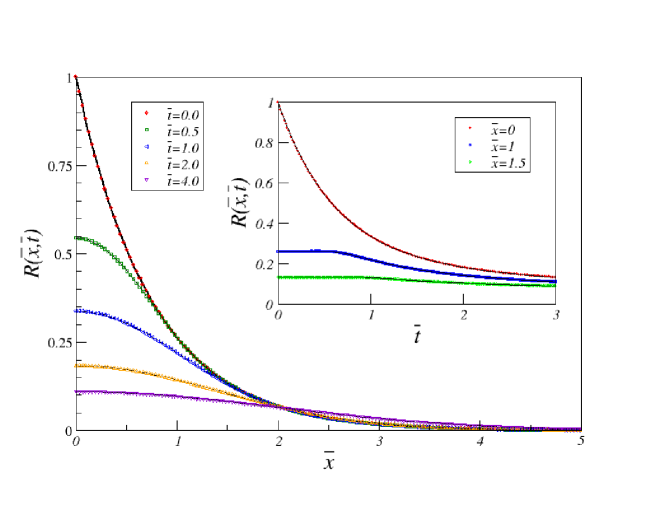
Refer to caption
Figure 7: The relaxation function Rโ€‹(xยฏ,tยฏ)๐‘…ยฏ๐‘ฅยฏ๐‘กR(\bar{x},\bar{t}) for fk=Aโ€‹eโˆ’ฮฒโ€‹k2subscript๐‘“๐‘˜๐ดsuperscripte๐›ฝsuperscript๐‘˜2f_{k}=A\,{\rm e}^{-\beta k^{2}} (where A=0.1๐ด0.1A=0.1 and ฮฒ=0.8๐›ฝ0.8\beta=0.8 have been used in this case) and Pa,b=1/9superscript๐‘ƒ๐‘Ž๐‘19P^{a,b}=1/9 for any choice of quantum numbers. Space and time are measured in unit of ฮพ๐œ‰\xi and ฯ„๐œ\tau respectively. Data points are numerical results and the solid line is the analytical prediction for the two-point function of a thermal initial state, see Eq. (52).

5 The dynamics of the transverse field Ising model

5.1 The paramagnetic phase

Another important check of formula (52) is represented by the transverse field Ising chain limit (TFIC). Briefly, we now focus on the dynamics after a quantum quench in the TFIC, whose Hamiltonian reads:

H^=โˆ’Jโ€‹(โˆ‘i=1Lโˆ’1ฯƒixโ€‹ฯƒi+1xโˆ’hโ€‹โˆ‘i=1Lฯƒiz),^๐ป๐ฝsuperscriptsubscript๐‘–1๐ฟ1superscriptsubscript๐œŽ๐‘–๐‘ฅsuperscriptsubscript๐œŽ๐‘–1๐‘ฅโ„Žsuperscriptsubscript๐‘–1๐ฟsuperscriptsubscript๐œŽ๐‘–๐‘ง\hat{H}=-J\left({\displaystyle\sum_{i=1}^{L-1}\sigma_{i}^{x}\sigma_{i+1}^{x}}-h{\displaystyle\sum_{i=1}^{L}\sigma_{i}^{z}}\right), (53)

where ฯƒiฮฑsuperscriptsubscript๐œŽ๐‘–๐›ผ\sigma_{i}^{\alpha} are the Pauli matrices at site i๐‘–i, J>0๐ฝ0J>0 is the energy scale, hโ„Žh the transverse magnetic field, and we impose free boundary conditions (for the moment we assume the system to be large but finite). The goal is to determine the dynamical order-parameter two-point function:

CIsingโ€‹(x,T,t)=โŸจฯˆ|ฯƒx2xโ€‹(t2)โ€‹ฯƒx1xโ€‹(t1)|ฯˆโŸฉ,superscript๐ถIsing๐‘ฅ๐‘‡๐‘กquantum-operator-product๐œ“superscriptsubscript๐œŽsubscript๐‘ฅ2๐‘ฅsubscript๐‘ก2superscriptsubscript๐œŽsubscript๐‘ฅ1๐‘ฅsubscript๐‘ก1๐œ“C^{\rm Ising}(x,T,t)=\langle\psi|\sigma_{x_{2}}^{x}(t_{2})\sigma_{x_{1}}^{x}(t_{1})|\psi\rangle, (54)

where x=x2โˆ’x1๐‘ฅsubscript๐‘ฅ2subscript๐‘ฅ1x=x_{2}-x_{1}, T=t1+t2๐‘‡subscript๐‘ก1subscript๐‘ก2T=t_{1}+t_{2} and t=t2โˆ’t1๐‘กsubscript๐‘ก2subscript๐‘ก1t=t_{2}-t_{1}. The action of the operator ฯƒixโ€‹(t)superscriptsubscript๐œŽ๐‘–๐‘ฅ๐‘ก\sigma_{i}^{x}(t) on the paramagnetic ground state is akin to that of the operator n~zsuperscript~๐‘›๐‘ง\tilde{n}^{z} in the O(3) non-linear sigma model, that is, it either creates an excitation or it destroys one already present. For this reason the semi-classical approach developed in the previous section is easily generalizable. For this model the K๐พK matrix in the definition of |ฯˆโŸฉket๐œ“|\psi\rangle is known and equal to Kโ€‹(k)=โˆ’i2โ€‹tanโก[ฮธkโˆ’ฮธkโ€ฒ2]๐พ๐‘˜๐‘–2subscript๐œƒ๐‘˜subscript๐œƒsuperscript๐‘˜โ€ฒ2K(k)=-\frac{i}{2}\tan\left[\frac{\theta_{k}-\theta_{k^{\prime}}}{2}\right], where the ฮธ๐œƒ\thetaโ€™s are the Bogoliubov angles defined in (57) before and after the quench respectively. In order to obtain (54), without rederiving everything from the beginning, one should formally replace Pa,b=1/(qโˆ’1)2superscript๐‘ƒ๐‘Ž๐‘1superscript๐‘ž12P^{a,b}=1/(q-1)^{2} and then take the limit qโ†’2โ†’๐‘ž2q\to 2. Otherwise we can start again from (33), and take into account that for the TFIC excitations do not have internal quantum numbers (this is true both in the ordered and disordered phases). This feature greatly simplifies the algebra of the derivation, and we end up with the following general expression for the correlator of equation (54), valid in the thermodynamic limit:

CIsingโ€‹(x,T,t)=CT=0Isingโ€‹(x,t)โ€‹expโก(โˆ’2โ€‹tโ€‹โˆซ0ฯ€dโ€‹kฯ€โ€‹fkโ€‹vkโ€‹ฮ˜โ€‹[vkโ€‹tโˆ’x])ร—expโก(โˆ’2โ€‹Tโ€‹โˆซ0ฯ€dโ€‹kฯ€โ€‹fkโ€‹vkโ€‹ฮ˜โ€‹[xโˆ’vkโ€‹T])โ€‹expโก(โˆ’2โ€‹xโ€‹โˆซ0ฯ€dโ€‹kฯ€โ€‹fkโ€‹ฮ˜โ€‹[xโˆ’vkโ€‹t]โ€‹ฮ˜โ€‹[vkโ€‹Tโˆ’x]),superscript๐ถIsing๐‘ฅ๐‘‡๐‘กsubscriptsuperscript๐ถIsing๐‘‡0๐‘ฅ๐‘ก2๐‘กsuperscriptsubscript0๐œ‹๐‘‘๐‘˜๐œ‹subscript๐‘“๐‘˜subscript๐‘ฃ๐‘˜ฮ˜delimited-[]subscript๐‘ฃ๐‘˜๐‘ก๐‘ฅabsent2๐‘‡superscriptsubscript0๐œ‹๐‘‘๐‘˜๐œ‹subscript๐‘“๐‘˜subscript๐‘ฃ๐‘˜ฮ˜delimited-[]๐‘ฅsubscript๐‘ฃ๐‘˜๐‘‡2๐‘ฅsuperscriptsubscript0๐œ‹๐‘‘๐‘˜๐œ‹subscript๐‘“๐‘˜ฮ˜delimited-[]๐‘ฅsubscript๐‘ฃ๐‘˜๐‘กฮ˜delimited-[]subscript๐‘ฃ๐‘˜๐‘‡๐‘ฅ\begin{array}[]{l}C^{\rm Ising}(x,T,t)=C^{\rm Ising}_{T=0}(x,t)\,\exp{\left(-2t{\displaystyle\int_{0}^{\pi}\frac{dk}{\pi}f_{k}v_{k}\Theta[v_{k}t-x]}\right)}\\ \qquad\qquad\times\exp{\left(-2T{\displaystyle\int_{0}^{\pi}\frac{dk}{\pi}f_{k}v_{k}\Theta[x-v_{k}T]}\right)}\exp{\left(-2x{\displaystyle\int_{0}^{\pi}\frac{dk}{\pi}f_{k}\Theta[x-v_{k}t]\Theta[v_{k}T-x]}\right)},\\ \end{array} (55)

where CT=0Isingโ€‹(x,t)subscriptsuperscript๐ถIsing๐‘‡0๐‘ฅ๐‘กC^{\rm Ising}_{T=0}(x,t) is given by (neglecting multi-particle terms in the spectral density [45]):

CT=0Isingโ€‹(x,t)โˆโˆซโˆ’ฯ€ฯ€dโ€‹k2โ€‹ฯ€โ€‹eโˆ’iโ€‹ฯตโ€‹(k)โ€‹t+iโ€‹kโ€‹xฯตโ€‹(k),proportional-tosubscriptsuperscript๐ถIsing๐‘‡0๐‘ฅ๐‘กsuperscriptsubscript๐œ‹๐œ‹๐‘‘๐‘˜2๐œ‹superscripte๐‘–italic-ฯต๐‘˜๐‘ก๐‘–๐‘˜๐‘ฅitalic-ฯต๐‘˜C^{\rm Ising}_{T=0}(x,t)\propto{\displaystyle\int_{-\pi}^{\pi}\frac{dk}{2\pi}\,\frac{{\rm e}^{-i\epsilon(k)t+ikx}}{\epsilon(k)}}, (56)

where again as long as we work on the lattice the energy-momentum relation is ฯตโ€‹(k)=[(hโˆ’cosโก(k))2+sin2โก(k)]1/2italic-ฯต๐‘˜superscriptdelimited-[]superscriptโ„Ž๐‘˜2superscript2๐‘˜12\epsilon(k)=[(h-\cos(k))^{2}+\sin^{2}(k)]^{1/2}. Once you take the proper scaling limit aโ†’0โ†’๐‘Ž0a\to 0, then ฯตโ€‹(k)italic-ฯต๐‘˜\epsilon(k) becomes relativistic and you can replace the general prefactor with a Bessel function K0subscript๐พ0K_{0}. Comparisons between theory and numerical data are shown in figures (8) and (9). We note that in expression (55) T๐‘‡T is arbitrary (with the constraint T>t>0๐‘‡๐‘ก0T>t>0), and not necessarily much longer than the Fermi time tf=x/vmโ€‹aโ€‹xsubscript๐‘ก๐‘“๐‘ฅsubscript๐‘ฃ๐‘š๐‘Ž๐‘ฅt_{f}=x/v_{max}, as was in (52).

Refer to caption
Refer to caption
Figure 8: The real and imaginary parts of the non-equal-time two point function after a quantum quench in the disordered phase, from h0=5subscriptโ„Ž05h_{0}=5 to h=2โ„Ž2h=2. By definition tยฏ=t/tfยฏ๐‘ก๐‘กsubscript๐‘ก๐‘“\bar{t}=t/t_{f} and Tยฏ=T/tfยฏ๐‘‡๐‘‡subscript๐‘ก๐‘“\bar{T}=T/t_{f}. Data points represent the numerical data extrapolated in the thermodynamic limit (Lโ†’โˆžโ†’๐ฟL\to\infty), while the solid line is given by equation (55). If we look at the inset in the plot of the real part, we notice that the semi-classical formula does not capture well the behaviour of the correlator outside of the light-cone (the same plot for the imaginary part shows a better agreement, even if at very small values of tยฏยฏ๐‘ก\bar{t} numerical errors do not allow us to compare analytical result with the numerical ones).

For larger quenches the semiclassical prediction, with fksubscript๐‘“๐‘˜f_{k} equal to |Kโ€‹(k)|2/(1+|Kโ€‹(k)|2)superscript๐พ๐‘˜21superscript๐พ๐‘˜2|K(k)|^{2}/(1+|K(k)|^{2}) is not accurate. Indeed one has to take into account that for arbitrary values of the magnetic field h>1โ„Ž1h>1 generic excitations are no longer single spin-flips (even if this is not the only source of error, see below).
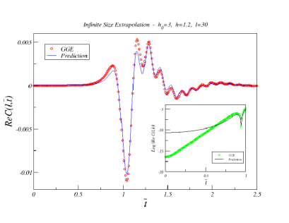
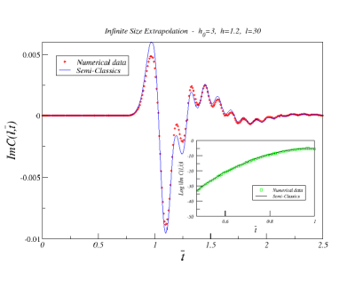
Refer to caption
Refer to caption
Figure 9: The real and imaginary parts of the non-equal-time two point function after a quantum quench in the disordered phase, from h0=3subscriptโ„Ž03h_{0}=3 to h=1.2โ„Ž1.2h=1.2. By definition tยฏ=t/tfยฏ๐‘ก๐‘กsubscript๐‘ก๐‘“\bar{t}=t/t_{f} and Tยฏ/tfโ‰ซ1much-greater-thanยฏ๐‘‡subscript๐‘ก๐‘“1\bar{T}/t_{f}\gg 1. Data points represent the numerical data extrapolated in the thermodynamic limit (Lโ†’โˆžโ†’๐ฟL\to\infty), while the solid line is given by equation (55). The same considerations made for (8) hold true here. In addition we notice that as this quench is closer to the critical point, the agreement is only qualitative at small tยฏยฏ๐‘ก\bar{t}, despite the substitution fkโ†’โˆ’1/2โ€‹logโก|cosโก(ฮ”k)|โ†’subscript๐‘“๐‘˜12subscriptฮ”๐‘˜f_{k}\to-1/2\log|\cos(\Delta_{k})|. To improve the agreement we should correct the expression for the pre-factor of equation (55), following the exact results of reference [61].

In general their shape is given by a superposition of states with an arbitrary number of spin-flips, with coefficients depending on the value of hโ„Žh itself. Only when hโ‰ซ1much-greater-thanโ„Ž1h\gg 1 are single excitations well-approximated by single-spin flips, as you treat them in the semi-classical approach. A first correction to the semiclassical results corresponds to substituting fkโ†’โˆ’1/2โ€‹logโก|cosโก(ฮ”k)|โ†’subscript๐‘“๐‘˜12subscriptฮ”๐‘˜f_{k}\to-1/2\log|\cos(\Delta_{k})|, where ฮ”ksubscriptฮ”๐‘˜\Delta_{k} is the Bogoliubov angle given by:

cosโก(ฮ”k)=h0โ€‹hโˆ’(h0+h)โ€‹cosโก(k)+1ฯตh0โ€‹(k)โ€‹ฯตhโ€‹(k).subscriptฮ”๐‘˜subscriptโ„Ž0โ„Žsubscriptโ„Ž0โ„Ž๐‘˜1subscriptitalic-ฯตsubscriptโ„Ž0๐‘˜subscriptitalic-ฯตโ„Ž๐‘˜\cos(\Delta_{k})={\displaystyle\frac{h_{0}h-(h_{0}+h)\cos(k)+1}{\epsilon_{h_{0}}(k)\epsilon_{h}(k)}}. (57)

This substitution, which follows from asymptotically exact techniques (see [40]), increases the agreement between the theoretical predictions and numerical data, expecially close to the quantum critical point h=1โ„Ž1h=1 where excitations are no longer localized objects. However in some plots mismatch between theory and numerics is still present, and we believe that it is due to the hypothesis of particle-number conservation of the pure semi-classical approach (i.e., the number of quasiparticles is conserved during the dynamical evolution of any configuration). If we considered the possibility of creating or destroying particles during the time evolution (which is realized by an operator insertion), we would get time-dependent corrections to the prefactor (56). Roughly speaking this would mean going beyond the leading order in the semi-classical approximation, a topic that is not addressed in detail in this paper. In the recent article [61] the dynamic correlators after a quantum quench were studied by using the form-factor technique, finding that the prefactor of expression (55) can be written as:

CT=0Isingโ€‹(x,t)โˆโˆซโˆ’ฯ€ฯ€dโ€‹k2โ€‹ฯ€โ€‹eiโ€‹kโ€‹xฯตโ€‹(k)โ€‹[eโˆ’iโ€‹ฯตkโ€‹t+2โ€‹iโ€‹tanโก(ฮ”k2)โ€‹cosโก(ฯตkโ€‹(T))โ€‹sgnโ€‹(xโˆ’ฯตkโ€ฒโ€‹t)].proportional-tosubscriptsuperscript๐ถIsing๐‘‡0๐‘ฅ๐‘กsuperscriptsubscript๐œ‹๐œ‹๐‘‘๐‘˜2๐œ‹superscripte๐‘–๐‘˜๐‘ฅitalic-ฯต๐‘˜delimited-[]superscripte๐‘–subscriptitalic-ฯต๐‘˜๐‘ก2๐‘–subscriptฮ”๐‘˜2subscriptitalic-ฯต๐‘˜๐‘‡sgn๐‘ฅsubscriptsuperscriptitalic-ฯตโ€ฒ๐‘˜๐‘กC^{\rm Ising}_{T=0}(x,t)\propto{\displaystyle\int_{-\pi}^{\pi}\frac{dk}{2\pi}\,\frac{{\rm e}^{ikx}}{\epsilon(k)}\left[{\rm e}^{-i\epsilon_{k}t}+2i\tan(\frac{\Delta_{k}}{2})\cos(\epsilon_{k}(T)){\rm sgn}(x-\epsilon^{\prime}_{k}t)\right]}. (58)

Outside the light-cone (when x>vmโ€‹aโ€‹xโ€‹t๐‘ฅsubscript๐‘ฃ๐‘š๐‘Ž๐‘ฅ๐‘กx>v_{max}t) the first contribution in (58) is exponentially small, whereas the second one behaves as a power law. This observation explains in turn why the pure semi-classical approximation typically fails when applied to this regime. In particular the semi-classics is not able to capture the behaviour of the equal-time correlator, that represents the extreme out-of-the light-cone case.

5.2 The ferromagnetic phase

Formula (52) cannot be directly used to derive the correlator of the Ising model in the ferromagnetic phase. In this case excitations are no longer spin-flips, in fact when h<1โ„Ž1h<1 these are domain walls (kinks). Following the general approach of F. Igloi and H. Reiger [37, 39] we can easily obtain the two-point correlation function for arbitrary value of times and distances. The key ideas of this method have already been extensively discussed in their works (even if these authors did not consider explicitly the case of dynamical correlators), here we just show the final result:

CIsingโ€‹(x,T,t)=Cโ€‹(h0,h)โ€‹Rโ€‹(x,T,t)superscript๐ถIsing๐‘ฅ๐‘‡๐‘ก๐ถsubscriptโ„Ž0โ„Ž๐‘…๐‘ฅ๐‘‡๐‘กC^{\rm Ising}(x,T,t)=C(h_{0},h)\,R(x,T,t) (59)

where the relaxation function in the ferromegnetic phase is equal to that in the paramagnetic phases while the multiplicative constant, as introduced in [42, 43] reads as:

Cโ€‹(h0,h)=1โˆ’hโ€‹h0+(1โˆ’h2)โ€‹(1โˆ’h02)2โ€‹1โˆ’hโ€‹h0โ€‹1โˆ’h024.๐ถsubscriptโ„Ž0โ„Ž1โ„Žsubscriptโ„Ž01superscriptโ„Ž21superscriptsubscriptโ„Ž0221โ„Žsubscriptโ„Ž041superscriptsubscriptโ„Ž02C(h_{0},h)={\displaystyle\frac{1-hh_{0}+\sqrt{(1-h^{2})(1-h_{0}^{2})}}{2\sqrt{1-hh_{0}}\sqrt[4]{1-h_{0}^{2}}}}. (60)

In addition it is worth noticing that the semi-classical two-point correlator in the ordered phase of the Ising model is always a real function, as was the dominant contribution of the form-factor result at large (x,T๐‘ฅ๐‘‡x,T) in [61]. In the ferromagnetic phase the equal-time correlators can also be described by the semi-classic approach, in contrast to the paramagnetic phase, as is shown in the inset of figure (10)
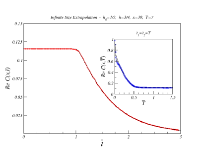
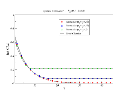
Refer to caption
Refer to caption
Figure 10: Left panel (inset): real part of the non-equal-time (equal-time) two point function in the ordered phase. Again the numerical data are extrapolated in the thermodynamic limit (Lโ†’โˆžโ†’๐ฟL\to\infty). In this phase, unlike in the paramagnetic one, the agreement between the semi-classics and the numerics works well also for the equal-time correlator. Right panel: spatial correlation at equal times.

6 Conclusions

We have developed a semi-classical theory for the out-of-equilibrium quantum relaxation of the O(3) non-linear sigma model, after having prepared the system in a coherent superposition of Cooper pairs, a structure that is in agreement with the integrability of the theory in the bulk. For such quenches we analyzed the two-point function of the order parameter n~zsubscript~๐‘›๐‘ง\tilde{n}_{z} and argued that, in the long time limit its expression is given by formula (52), while for arbitrary times by equation (76). The method employed here is a generalization of that used for studying the finite-temperature behaviour of a series of one-dimensional chains [49, 50, 57]. As was already observed in other integrable models, the long-time behaviour of this two-point function after a quantum quench is not thermal. For equal times (t2=t1โ‰ซx/vmโ€‹aโ€‹xsubscript๐‘ก2subscript๐‘ก1much-greater-than๐‘ฅsubscript๐‘ฃ๐‘š๐‘Ž๐‘ฅt_{2}=t_{1}\gg x/v_{max}) the relaxation (52) reaches a stationary state, while for non-equal times (t2โ‰ t1subscript๐‘ก2subscript๐‘ก1t_{2}\neq t_{1}) it is expressed as a function of the time difference t๐‘กt. These features are strong indications that the long-time limit of the two-point function (7) can be described by a statistical ensemble, and we expect it to be the GGE, being the model integrable. It would be interesting to have an independent and explicit result in the GGE framework, in order to check the general belief also for the O(3) non-linear sigma model. The main difficulty here consists in finding an analytical expression for the lagrangian parameters of the GGE Hamiltonian, in order to explicitly carry out the statistical average.
The semi-classical approach has also been applied to predict the dynamics of the order-parameter two-point function of the transverse field Ising chain, in both phases. In this case results for the auto-correlation and for the equal-time correlation are already present in literature [30, 37], the novelty here is the generalization of the semi-classical method to the case of different-times correlators. Yet, the exact results recently obtained in [61], have allowed us to explore the limit of the pure semi-classics. This technique works very well within the ferromagnetic phase (also for pretty large quenches), whilst it is in the paramagnetic phase where it shows its real limits: it fails in predicting the equal-time two-point correlation functions, and in general the agreement in the out-of-the-light-cone case (see the insets of figures (8) and (9)) is only qualitative. Furthermore in the proximity of the critical point, the method - which in general is supposed to work well only for small quenches - needs to be improved with the substitution fkโ†’โˆ’1/2โ€‹logโก|cosโก(ฮ”k)|โ†’subscript๐‘“๐‘˜12subscriptฮ”๐‘˜f_{k}\to-1/2\log|\cos(\Delta_{k})|, which takes into account the real shape of the excitations.
Nevertheless, our semi-classical theory can be applied straightforwardly to several other models, integrable and non-integrable, including the q-Potts model and the sine-Gordon theory, in order to compute correlators. These models will generate different combinatorial problems (the nature of the excitations is, of course, model-dependent), but the main ideas remain the same.

I am extremely grateful to Fabian Essler for the suggestion of working on this problem and for all the instructive discussions we have had over the last year. Without his support this work would have never seen the light of day. I am also in great debt to Maurizio Fagotti for his priceless help and for the huge number of useful hints he gave me.
Finally I want to thank N.J. Robinson, J. Cardy, A.M. Tsvelik, R.M. Konik and S. Sotiriadis for fruitful and pleasant discussions.

Appendix A Occupation numbers and mode probabilities

In this appendix we compute the occupation numbers and the probability distributions for each mode, starting from the definition of the squeezed coherent state (3) and the operator algebra of the operators (Z,Zโ€ )๐‘superscript๐‘โ€ (Z,Z^{{\dagger}}). Let us recall the definition of the initial state |ฯˆโŸฉket๐œ“|\psi\rangle:

|ฯˆโŸฉ=expโก(โˆ‘a,bโˆซ0โˆždโ€‹k2โ€‹ฯ€โ€‹Kaโ€‹bโ€‹(k)โ€‹Zaโ€ โ€‹(โˆ’k)โ€‹Zbโ€ โ€‹(k))โ€‹|0โŸฉ,ket๐œ“subscript๐‘Ž๐‘superscriptsubscript0๐‘‘๐‘˜2๐œ‹superscript๐พ๐‘Ž๐‘๐‘˜subscriptsuperscript๐‘โ€ ๐‘Ž๐‘˜subscriptsuperscript๐‘โ€ ๐‘๐‘˜ket0|\psi\rangle=\exp{\left(\sum_{a,b}\int_{0}^{\infty}\frac{dk}{2\pi}\,K^{ab}(k)Z^{{\dagger}}_{a}(-k)Z^{{\dagger}}_{b}(k)\right)}|0\rangle, (61)

The Z๐‘Z operators obey the Zamolodchikov-Faddeev (ZF) algebra, namely:

Zaโ€‹(k1)โ€‹Zbโ€‹(k2)โˆ’๐’ฎaโ€‹bcโ€‹dโ€‹(k1,k2)โ€‹Zdโ€‹(k2)โ€‹Zcโ€‹(k1)=0Zaโ€ โ€‹(k1)โ€‹Zbโ€ โ€‹(k2)โˆ’๐’ฎaโ€‹bcโ€‹dโ€‹(k1,k2)โ€‹Zdโ€ โ€‹(k2)โ€‹Zcโ€ โ€‹(k1)=0Zaโ€‹(k1)โ€‹Zbโ€ โ€‹(k2)โˆ’๐’ฎcโ€‹baโ€‹dโ€‹(k1,k2)โ€‹Zdโ€ โ€‹(k2)โ€‹Zcโ€‹(k1)=ฮดaโ€‹bโ€‹ฮดโ€‹(k1โˆ’k2).subscript๐‘๐‘Žsubscript๐‘˜1subscript๐‘๐‘subscript๐‘˜2superscriptsubscript๐’ฎ๐‘Ž๐‘๐‘๐‘‘subscript๐‘˜1subscript๐‘˜2subscript๐‘๐‘‘subscript๐‘˜2subscript๐‘๐‘subscript๐‘˜10superscriptsubscript๐‘๐‘Žโ€ subscript๐‘˜1superscriptsubscript๐‘๐‘โ€ subscript๐‘˜2superscriptsubscript๐’ฎ๐‘Ž๐‘๐‘๐‘‘subscript๐‘˜1subscript๐‘˜2superscriptsubscript๐‘๐‘‘โ€ subscript๐‘˜2superscriptsubscript๐‘๐‘โ€ subscript๐‘˜10subscript๐‘๐‘Žsubscript๐‘˜1superscriptsubscript๐‘๐‘โ€ subscript๐‘˜2superscriptsubscript๐’ฎ๐‘๐‘๐‘Ž๐‘‘subscript๐‘˜1subscript๐‘˜2superscriptsubscript๐‘๐‘‘โ€ subscript๐‘˜2subscript๐‘๐‘subscript๐‘˜1subscript๐›ฟ๐‘Ž๐‘๐›ฟsubscript๐‘˜1subscript๐‘˜2\begin{array}[]{l}Z_{a}(k_{1})Z_{b}(k_{2})-\mathcal{S}_{ab}^{cd}(k_{1},k_{2})Z_{d}(k_{2})Z_{c}(k_{1})=0\\ Z_{a}^{{\dagger}}(k_{1})Z_{b}^{{\dagger}}(k_{2})-\mathcal{S}_{ab}^{cd}(k_{1},k_{2})Z_{d}^{{\dagger}}(k_{2})Z_{c}^{{\dagger}}(k_{1})=0\\ Z_{a}(k_{1})Z_{b}^{{\dagger}}(k_{2})-\mathcal{S}_{cb}^{ad}(k_{1},k_{2})Z_{d}^{{\dagger}}(k_{2})Z_{c}(k_{1})=\delta_{ab}\,\delta(k_{1}-k_{2}).\end{array} (62)

Intuitively this means that the exchange of two quasiparticle is realized by the two-particle scattering matrix ๐’ฎโ€‹(k1,k2)๐’ฎsubscript๐‘˜1subscript๐‘˜2\mathcal{S}(k_{1},k_{2}). In the present case we assume the form (18) for the ๐’ฎ๐’ฎ\mathcal{S} matrix, and thus the ZF algebra becomes:

Zaโ€‹(k1)โ€‹Zbโ€‹(k2)+Zaโ€‹(k2)โ€‹Zbโ€‹(k1)=0Zaโ€ โ€‹(k1)โ€‹Zbโ€ โ€‹(k2)+Zaโ€ โ€‹(k2)โ€‹Zbโ€ โ€‹(k1)=0Zaโ€‹(k1)โ€‹Zbโ€ โ€‹(k2)=[โˆ’โˆ‘cZcโ€ โ€‹(k2)โ€‹Zcโ€‹(k1)+ฮดโ€‹(k1โˆ’k2)]โ€‹ฮดaโ€‹b.subscript๐‘๐‘Žsubscript๐‘˜1subscript๐‘๐‘subscript๐‘˜2subscript๐‘๐‘Žsubscript๐‘˜2subscript๐‘๐‘subscript๐‘˜10superscriptsubscript๐‘๐‘Žโ€ subscript๐‘˜1superscriptsubscript๐‘๐‘โ€ subscript๐‘˜2superscriptsubscript๐‘๐‘Žโ€ subscript๐‘˜2superscriptsubscript๐‘๐‘โ€ subscript๐‘˜10subscript๐‘๐‘Žsubscript๐‘˜1superscriptsubscript๐‘๐‘โ€ subscript๐‘˜2delimited-[]subscript๐‘superscriptsubscript๐‘๐‘โ€ subscript๐‘˜2subscript๐‘๐‘subscript๐‘˜1๐›ฟsubscript๐‘˜1subscript๐‘˜2subscript๐›ฟ๐‘Ž๐‘\begin{array}[]{l}Z_{a}(k_{1})Z_{b}(k_{2})+Z_{a}(k_{2})Z_{b}(k_{1})=0\\ Z_{a}^{{\dagger}}(k_{1})Z_{b}^{{\dagger}}(k_{2})+Z_{a}^{{\dagger}}(k_{2})Z_{b}^{{\dagger}}(k_{1})=0\\ Z_{a}(k_{1})Z_{b}^{{\dagger}}(k_{2})=[-\sum_{c}Z_{c}^{{\dagger}}(k_{2})Z_{c}(k_{1})+\delta(k_{1}-k_{2})]\delta_{ab}.\end{array} (63)

The ground state |0โŸฉket0|0\rangle satisfies Zaโ€‹(k)โ€‹|0โŸฉ=0subscript๐‘๐‘Ž๐‘˜ket00Z_{a}(k)|0\rangle=0, โˆ€afor-all๐‘Ž\forall{a} โˆ€kfor-all๐‘˜\forall{k}. From equations (62) it is clear that this algebra encodes the fact that the order of quantum number is preserved in time. The main quantities we want to compute are the occupation numbers fkaโ€‹bsuperscriptsubscript๐‘“๐‘˜๐‘Ž๐‘f_{k}^{ab}, which are defined by:

โŸจฯˆ|Zaโ€ โ€‹(โˆ’k)โ€‹Zbโ€ โ€‹(k)โ€‹Zbโ€‹(k)โ€‹Zaโ€‹(โˆ’k)|ฯˆโŸฉโŸจฯˆ|ฯˆโŸฉโ‰กfkaโ€‹b.quantum-operator-product๐œ“superscriptsubscript๐‘๐‘Žโ€ ๐‘˜superscriptsubscript๐‘๐‘โ€ ๐‘˜subscript๐‘๐‘๐‘˜subscript๐‘๐‘Ž๐‘˜๐œ“inner-product๐œ“๐œ“superscriptsubscript๐‘“๐‘˜๐‘Ž๐‘\frac{\langle\psi|Z_{a}^{{\dagger}}(-k)Z_{b}^{{\dagger}}(k)Z_{b}(k)Z_{a}(-k)|\psi\rangle}{\langle\psi|\psi\rangle}\equiv f_{k}^{ab}. (64)

This quantity is exactly the number of quasiparticle pairs of kind (a,b)๐‘Ž๐‘(a,b) with momenta (โˆ’k,k)๐‘˜๐‘˜(-k,k) (see figure (3)), and it is directly connected to the probabilities Pฮปโ€‹ฮปโ€ฒsuperscript๐‘ƒ๐œ†superscript๐œ†โ€ฒP^{\lambda\lambda^{\prime}} we defined in the body of the paper. The idea is to treat the K๐พK-matrix as an expansion parameter, but working from the beginning in the thermodynamic limit the squeezed state does not have a good expansion. Divergences appear in the expansion terms, in the form of square Dirac delta-functions. In general there are two different methods of regularizing these divergences: one directly regulates the integral expressions in the infinite volume whereas the other operates through subtracting divergences in a large, finite volume. These two techniques were proposed and compared in [63]. In the follow we shall use the second method.
Let us start by analysing the expansion of the denominator of (64). First Taylor expand the squezeed state as:

|ฯˆโŸฉ=(1+โˆ‘a,bk>0Kaโ€‹bโ€‹(k)โ€‹Zaโ€ โ€‹(โˆ’k)โ€‹Zbโ€ โ€‹(k)+12!โ€‹(โˆ‘a,bk>0Kaโ€‹bโ€‹(k)โ€‹Zaโ€ โ€‹(โˆ’k)โ€‹Zbโ€ โ€‹(k))2+โ€ฆ)โ€‹|0โŸฉ,ket๐œ“1subscriptsuperscript๐‘Ž๐‘๐‘˜0superscript๐พ๐‘Ž๐‘๐‘˜subscriptsuperscript๐‘โ€ ๐‘Ž๐‘˜subscriptsuperscript๐‘โ€ ๐‘๐‘˜12superscriptsubscriptsuperscript๐‘Ž๐‘๐‘˜0superscript๐พ๐‘Ž๐‘๐‘˜subscriptsuperscript๐‘โ€ ๐‘Ž๐‘˜subscriptsuperscript๐‘โ€ ๐‘๐‘˜2โ€ฆket0|\psi\rangle=(1+\sum_{\stackrel{{\scriptstyle k>0}}{{a,b}}}K^{ab}(k)Z^{{\dagger}}_{a}(-k)Z^{{\dagger}}_{b}(k)+\frac{1}{2!}(\sum_{\stackrel{{\scriptstyle k>0}}{{a,b}}}K^{ab}(k)Z^{{\dagger}}_{a}(-k)Z^{{\dagger}}_{b}(k))^{2}+\dots)|0\rangle, (65)

therefore we have:

โŸจฯˆ|ฯˆโŸฉ=1+Z1+Z2+โ€ฆ,inner-product๐œ“๐œ“1subscript๐‘1subscript๐‘2โ€ฆ\langle\psi|\psi\rangle=1+Z_{1}+Z_{2}+\dots, (66)

where

Z1=โˆ‘a,bk>0โˆ‘c,dฮพ>0(Kaโ€‹bโ€‹(k))โˆ—โ€‹Kcโ€‹dโ€‹(ฮพ)โ€‹โŸจ0|Zbโ€‹(k)โ€‹Zaโ€‹(โˆ’k)โ€‹Zcโ€ โ€‹(โˆ’ฮพ)โ€‹Zdโ€ โ€‹(ฮพ)|0โŸฉ=โˆ‘a,bk>0|Kaโ€‹bโ€‹(k)|2.subscript๐‘1subscriptsuperscript๐‘Ž๐‘๐‘˜0subscriptsuperscript๐‘๐‘‘๐œ‰0superscriptsuperscript๐พ๐‘Ž๐‘๐‘˜superscript๐พ๐‘๐‘‘๐œ‰quantum-operator-product0subscript๐‘๐‘๐‘˜subscript๐‘๐‘Ž๐‘˜superscriptsubscript๐‘๐‘โ€ ๐œ‰superscriptsubscript๐‘๐‘‘โ€ ๐œ‰0subscriptsuperscript๐‘Ž๐‘๐‘˜0superscriptsuperscript๐พ๐‘Ž๐‘๐‘˜2Z_{1}=\sum_{\stackrel{{\scriptstyle k>0}}{{a,b}}}\sum_{\stackrel{{\scriptstyle\xi>0}}{{c,d}}}(K^{ab}(k))^{*}K^{cd}(\xi)\langle 0|Z_{b}(k)Z_{a}(-k)Z_{c}^{{\dagger}}(-\xi)Z_{d}^{{\dagger}}(\xi)|0\rangle=\sum_{\stackrel{{\scriptstyle k>0}}{{a,b}}}|K^{ab}(k)|^{2}. (67)

As expected this term is proportional to the volume L๐ฟL. the higher orders will be proportional to L2superscript๐ฟ2L^{2}, L3superscript๐ฟ3L^{3} et cetera. Let us consider the expansion of the numerator of (64):

โŸจฯˆ|Zฮฑโ€ โ€‹(โˆ’ฮพ)โ€‹Zฮฒโ€ โ€‹(ฮพ)โ€‹Zฮฒโ€‹(ฮพ)โ€‹Zฮฑโ€‹(โˆ’ฮพ)|ฯˆโŸฉ=W1+14โ€‹W2+โ€ฆ,quantum-operator-product๐œ“superscriptsubscript๐‘๐›ผโ€ ๐œ‰superscriptsubscript๐‘๐›ฝโ€ ๐œ‰subscript๐‘๐›ฝ๐œ‰subscript๐‘๐›ผ๐œ‰๐œ“subscript๐‘Š114subscript๐‘Š2โ€ฆ\langle\psi|Z_{\alpha}^{{\dagger}}(-\xi)Z_{\beta}^{{\dagger}}(\xi)Z_{\beta}(\xi)Z_{\alpha}(-\xi)|\psi\rangle=W_{1}+\frac{1}{4}W_{2}+\dots, (68)

where the first term W1subscript๐‘Š1W_{1}is given by:

W1=โˆ‘a,bk1>0โˆ‘c,dk2>0โŸจ0|Zcโ€‹(k2)โ€‹Zdโ€‹(โˆ’k2)โ€‹Zฮฑโ€ โ€‹(โˆ’ฮพ)โ€‹Zฮฒโ€ โ€‹(ฮพ)โ€‹Zฮฒโ€‹(ฮพ)โ€‹Zฮฑโ€‹(โˆ’ฮพ)โ€‹Zaโ€ โ€‹(โˆ’k1)โ€‹Zbโ€ โ€‹(k1)|0โŸฉ=|Kฮฑโ€‹ฮฒโ€‹(ฮพ)|2.subscript๐‘Š1subscriptsuperscript๐‘Ž๐‘subscript๐‘˜10subscriptsuperscript๐‘๐‘‘subscript๐‘˜20quantum-operator-product0subscript๐‘๐‘subscript๐‘˜2subscript๐‘๐‘‘subscript๐‘˜2superscriptsubscript๐‘๐›ผโ€ ๐œ‰superscriptsubscript๐‘๐›ฝโ€ ๐œ‰subscript๐‘๐›ฝ๐œ‰subscript๐‘๐›ผ๐œ‰superscriptsubscript๐‘๐‘Žโ€ subscript๐‘˜1superscriptsubscript๐‘๐‘โ€ subscript๐‘˜10superscriptsuperscript๐พ๐›ผ๐›ฝ๐œ‰2W_{1}=\sum_{\stackrel{{\scriptstyle k_{1}>0}}{{a,b}}}\sum_{\stackrel{{\scriptstyle k_{2}>0}}{{c,d}}}\langle 0|Z_{c}(k_{2})Z_{d}(-k_{2})Z_{\alpha}^{{\dagger}}(-\xi)Z_{\beta}^{{\dagger}}(\xi)Z_{\beta}(\xi)Z_{\alpha}(-\xi)Z_{a}^{{\dagger}}(-k_{1})Z_{b}^{{\dagger}}(k_{1})|0\rangle=|K^{\alpha\beta}(\xi)|^{2}. (69)

This quantity is finite, also in the infinite volume limit Lโ†’โˆžโ†’๐ฟL\to\infty, whilst W2subscript๐‘Š2W_{2} is proportional to L๐ฟL. We now need the expression of W2subscript๐‘Š2W_{2} to see how these divergences cancel against the normalization of the boundary state. By definition we have:

W2=โˆ‘a,bk1>0โˆ‘c,dk2>0โˆ‘e,fk3>0โˆ‘g,hk4>0โŸจ0|โ€‹Zaโ€‹(k1)โ€‹Zbโ€‹(โˆ’k1)โ€‹Zcโ€‹(k2)โ€‹Zdโ€‹(โˆ’k2)โ€‹Zฮฑโ€ โ€‹(โˆ’ฮพ)โ€‹Zฮฒโ€ โ€‹(ฮพ)ร—Zฮฒโ€‹(ฮพ)โ€‹Zฮฑโ€‹(โˆ’ฮพ)โ€‹Zeโ€ โ€‹(โˆ’k3)โ€‹Zfโ€ โ€‹(k3)โ€‹Zgโ€ โ€‹(โˆ’k4)โ€‹Zhโ€ โ€‹(k4)โ€‹|0โŸฉsubscript๐‘Š2subscriptsuperscript๐‘Ž๐‘subscript๐‘˜10subscriptsuperscript๐‘๐‘‘subscript๐‘˜20subscriptsuperscript๐‘’๐‘“subscript๐‘˜30subscriptsuperscript๐‘”โ„Žsubscript๐‘˜40bra0subscript๐‘๐‘Žsubscript๐‘˜1subscript๐‘๐‘subscript๐‘˜1subscript๐‘๐‘subscript๐‘˜2subscript๐‘๐‘‘subscript๐‘˜2superscriptsubscript๐‘๐›ผโ€ ๐œ‰superscriptsubscript๐‘๐›ฝโ€ ๐œ‰absentsubscript๐‘๐›ฝ๐œ‰subscript๐‘๐›ผ๐œ‰superscriptsubscript๐‘๐‘’โ€ subscript๐‘˜3superscriptsubscript๐‘๐‘“โ€ subscript๐‘˜3superscriptsubscript๐‘๐‘”โ€ subscript๐‘˜4superscriptsubscript๐‘โ„Žโ€ subscript๐‘˜4ket0\begin{array}[]{l}W_{2}={\displaystyle\sum_{\stackrel{{\scriptstyle k_{1}>0}}{{a,b}}}\sum_{\stackrel{{\scriptstyle k_{2}>0}}{{c,d}}}\sum_{\stackrel{{\scriptstyle k_{3}>0}}{{e,f}}}\sum_{\stackrel{{\scriptstyle k_{4}>0}}{{g,h}}}\langle 0|Z_{a}(k_{1})Z_{b}(-k_{1})Z_{c}(k_{2})Z_{d}(-k_{2})Z_{\alpha}^{{\dagger}}(-\xi)Z_{\beta}^{{\dagger}}(\xi)}\\ {\displaystyle\times Z_{\beta}(\xi)Z_{\alpha}(-\xi)Z_{e}^{{\dagger}}(-k_{3})Z_{f}^{{\dagger}}(k_{3})Z_{g}^{{\dagger}}(-k_{4})Z_{h}^{{\dagger}}(k_{4})|0\rangle}\end{array} (70)

After a bit of algebra we end up with the following result for W2subscript๐‘Š2W_{2}:

W2=4โ€‹|Kฮฑโ€‹ฮฒโ€‹(ฮพ)|2โ€‹โˆ‘a,bk>0|Kaโ€‹bโ€‹(k)|2+2โ€‹|Kฮฑโ€‹ฮฒโ€‹(ฮพ)|2โ€‹โˆ‘a,b|Kaโ€‹bโ€‹(ฮพ)|2,subscript๐‘Š24superscriptsuperscript๐พ๐›ผ๐›ฝ๐œ‰2subscriptsuperscript๐‘Ž๐‘๐‘˜0superscriptsuperscript๐พ๐‘Ž๐‘๐‘˜22superscriptsuperscript๐พ๐›ผ๐›ฝ๐œ‰2subscript๐‘Ž๐‘superscriptsuperscript๐พ๐‘Ž๐‘๐œ‰2W_{2}={\displaystyle 4|K^{\alpha\beta}(\xi)|^{2}\sum_{\stackrel{{\scriptstyle k>0}}{{a,b}}}|K^{ab}(k)|^{2}+2|K^{\alpha\beta}(\xi)|^{2}\sum_{a,b}|K^{ab}(\xi)|^{2}}, (71)

where we immediately see that the first term is of order L๐ฟL. In particular the first term of (70) can be written as 4โ€‹W1โ€‹Z14subscript๐‘Š1subscript๐‘14W_{1}Z_{1}, thus the first correction in equation (64) is given by:

โŸจฯˆ|Zaโ€ โ€‹(โˆ’k)โ€‹Zbโ€ โ€‹(k)โ€‹Zbโ€‹(k)โ€‹Zaโ€‹(โˆ’k)|ฯˆโŸฉโŸจฯˆ|ฯˆโŸฉ=W1โ€‹(1+Z1)1+Z1+โ€ฆ=W1+oโ€‹(W1).quantum-operator-product๐œ“superscriptsubscript๐‘๐‘Žโ€ ๐‘˜superscriptsubscript๐‘๐‘โ€ ๐‘˜subscript๐‘๐‘๐‘˜subscript๐‘๐‘Ž๐‘˜๐œ“inner-product๐œ“๐œ“subscript๐‘Š11subscript๐‘11subscript๐‘1โ€ฆsubscript๐‘Š1๐‘œsubscript๐‘Š1\frac{\langle\psi|Z_{a}^{{\dagger}}(-k)Z_{b}^{{\dagger}}(k)Z_{b}(k)Z_{a}(-k)|\psi\rangle}{\langle\psi|\psi\rangle}={\displaystyle\frac{W_{1}(1+Z_{1})}{1+Z_{1}}}+\dots=W_{1}+o(W_{1}). (72)

We see that the divergent term indeed cancels against the normalization factor, and this happens order by order. We conclude that as long as Kaโ€‹bโ€‹(k)superscript๐พ๐‘Ž๐‘๐‘˜K^{ab}(k) is small we can calculate the matrix elements like (64) by expanding the squeezed state. The final result can be written as:

\boxedโ€‹fkaโ€‹b=|Kaโ€‹bโ€‹(k)|2+oโ€‹(|Kaโ€‹bโ€‹(k)|2)\boxedsuperscriptsubscript๐‘“๐‘˜๐‘Ž๐‘superscriptsuperscript๐พ๐‘Ž๐‘๐‘˜2๐‘œsuperscriptsuperscript๐พ๐‘Ž๐‘๐‘˜2\boxed{f_{k}^{ab}=|K^{ab}(k)|^{2}+o(|K^{ab}(k)|^{2})} (73)

which explains the name amplitudes for the matrix elements Kaโ€‹bโ€‹(k)superscript๐พ๐‘Ž๐‘๐‘˜K^{ab}(k). The momentum occupation numbers fksubscript๐‘“๐‘˜f_{k} are given by:

fk=โˆ‘a,bfkaโ€‹b,subscript๐‘“๐‘˜subscript๐‘Ž๐‘superscriptsubscript๐‘“๐‘˜๐‘Ž๐‘f_{k}=\sum_{a,b}f_{k}^{ab}, (74)

while for the probability densities Paโ€‹bโ€‹(k)superscript๐‘ƒ๐‘Ž๐‘๐‘˜P^{ab}(k) -which are defined in the thermodynamic limit- we have:

Paโ€‹bโ€‹(k)=fkaโ€‹bโˆ‘a,bโˆซ0โˆždโ€‹k2โ€‹ฯ€โ€‹fkaโ€‹b,superscript๐‘ƒ๐‘Ž๐‘๐‘˜superscriptsubscript๐‘“๐‘˜๐‘Ž๐‘subscript๐‘Ž๐‘superscriptsubscript0๐‘‘๐‘˜2๐œ‹superscriptsubscript๐‘“๐‘˜๐‘Ž๐‘P^{ab}(k)=\frac{{\displaystyle f_{k}^{ab}}}{{\displaystyle\sum_{a,b}\int_{0}^{\infty}\frac{dk}{2\pi}f_{k}^{ab}}}, (75)

which makes the normalization condition โˆ‘a,bโˆซ0โˆždโ€‹k2โ€‹ฯ€โ€‹Paโ€‹bโ€‹(k)=1subscript๐‘Ž๐‘superscriptsubscript0๐‘‘๐‘˜2๐œ‹superscript๐‘ƒ๐‘Ž๐‘๐‘˜1\sum_{a,b}\int_{0}^{\infty}\frac{dk}{2\pi}P^{ab}(k)=1 explicit. The probability Paโ€‹bsuperscript๐‘ƒ๐‘Ž๐‘P^{ab} is defined by Paโ€‹b=โˆซ0โˆždโ€‹k2โ€‹ฯ€โ€‹Paโ€‹bโ€‹(k)superscript๐‘ƒ๐‘Ž๐‘superscriptsubscript0๐‘‘๐‘˜2๐œ‹superscript๐‘ƒ๐‘Ž๐‘๐‘˜P^{ab}=\int_{0}^{\infty}\frac{dk}{2\pi}P^{ab}(k).

Appendix B General expression of the relaxation function Rโ€‹(r,t,T)๐‘…๐‘Ÿ๐‘ก๐‘‡R(r,t,T)

In this appendix we show the form of the relaxation function for the O(3) non-linear sigma model when the times T๐‘‡T and t๐‘กt are arbitrary, with the only constraint T>t>0๐‘‡๐‘ก0T>t>0. This expression can be written as:

Rโ€‹(r;t,T)=R1โ€‹(r;t,T)+R2โ€‹(r;t,T),๐‘…๐‘Ÿ๐‘ก๐‘‡subscript๐‘…1๐‘Ÿ๐‘ก๐‘‡subscript๐‘…2๐‘Ÿ๐‘ก๐‘‡R(r;t,T)=R_{1}(r;t,T)+R_{2}(r;t,T), (76)

where the first addend reads as:

R1โ€‹(r;t,T)=โˆซโˆ’ฯ€ฯ€dโ€‹ฯ•2โ€‹ฯ€โ€‹expโก(โˆ’tโ€‹(1โˆ’cosโกฯ•)โ€‹โˆซ0โˆždโ€‹kฯ€โ€‹fkโ€‹vkโ€‹ฮ˜โ€‹[vkโ€‹tโˆ’r])ร—expโก(โˆ’Tโ€‹(1+cosโก2โ€‹ฯ•โˆ’2โ€‹cosโกฯ•)โ€‹โˆซ0โˆždโ€‹k2โ€‹ฯ€โ€‹fkโ€‹vkโ€‹ฮ˜โ€‹[rโˆ’vkโ€‹T])ร—expโก(โˆ’rโ€‹(1โˆ’cosโกฯ•)โ€‹โˆซ0โˆždโ€‹kฯ€โ€‹fkโ€‹ฮ˜โ€‹[rโˆ’vkโ€‹t]โ€‹ฮ˜โ€‹[vkโ€‹Tโˆ’r])ร—expโก(โˆ’rโ€‹(1โˆ’cosโก2โ€‹ฯ•)โ€‹โˆซ0โˆždโ€‹k2โ€‹ฯ€โ€‹fkโ€‹ฮ˜โ€‹[rโˆ’vkโ€‹T])ร—cos{rsin2ฯ•โˆซ0โˆždโ€‹k2โ€‹ฯ€fkฮ˜[rโˆ’vkT]+rsinฯ•โˆซ0โˆždโ€‹kฯ€fkฮ˜[vkTโˆ’r]+2T(sinฯ•โˆ’sin2ฯ•)โˆซ0โˆždโ€‹k2โ€‹ฯ€fkvkฮ˜[rโˆ’vkT]}ร—1+2โ€‹cosโก(ฯ•)โ€‹(P00โˆ’1)โ€‹Q+cosโก(2โ€‹ฯ•)โ€‹(Q2โˆ’P00)โˆ’P00โ€‹Q21โˆ’2โ€‹P00โ€‹cosโก(2โ€‹ฯ•)+(P00)2,\begin{array}[]{l}\quad R_{1}(r;t,T)={\displaystyle\int_{-\pi}^{\pi}\frac{d\phi}{2\pi}}\exp{\left(-t(1-\cos\phi){\displaystyle\int_{0}^{\infty}\frac{dk}{\pi}f_{k}\,v_{k}\Theta[v_{k}t-r]}\right)}\\ \quad\times\exp{\left(-T(1+\cos 2\phi-2\cos\phi){\displaystyle\int_{0}^{\infty}\frac{dk}{2\pi}f_{k}v_{k}\,\Theta[r-v_{k}T]}\right)}\\ \quad\times\exp{\left(-r(1-\cos\phi){\displaystyle\int_{0}^{\infty}\frac{dk}{\pi}f_{k}\,\Theta[r-v_{k}t]\Theta[v_{k}T-r]}\right)}\\ \quad\times\exp{\left(-r(1-\cos 2\phi){\displaystyle\int_{0}^{\infty}\frac{dk}{2\pi}f_{k}\,\Theta[r-v_{k}T]}\right)}\\ \quad\times\cos\left\{r\sin 2\phi{\displaystyle\int_{0}^{\infty}\frac{dk}{2\pi}f_{k}\Theta[r-v_{k}T]+r\sin\phi\int_{0}^{\infty}\frac{dk}{\pi}f_{k}\Theta[v_{k}T-r]}\right.\\ \quad+\left.2T(\sin\phi-\sin 2\phi){\displaystyle\int_{0}^{\infty}\frac{dk}{2\pi}f_{k}v_{k}\,\Theta[r-v_{k}T]}\right\}\\ \quad\times{\displaystyle\frac{1+2\cos(\phi)(P^{00}-1)Q+\cos(2\phi)(Q^{2}-P^{00})-P^{00}Q^{2}}{1-2P^{00}\cos(2\phi)+(P^{00})^{2}}}\\ ,\end{array} (77)

and the second term is given by

R2โ€‹(r;t,T)=โˆซโˆ’ฯ€ฯ€dโ€‹ฯ•2โ€‹ฯ€โ€‹expโก(โˆ’2โ€‹(Tโˆ’tโ€‹cosโกฯ•)โ€‹โˆซ0โˆždโ€‹k2โ€‹ฯ€โ€‹fkโ€‹vkโ€‹ฮ˜โ€‹[vkโ€‹Tโˆ’r])ร—expโก(โˆ’rโ€‹(1โˆ’cosโก2โ€‹ฯ•)โ€‹โˆซ0โˆždโ€‹k2โ€‹ฯ€โ€‹fkโ€‹ฮ˜โ€‹[rโˆ’vkโ€‹T])ร—expโก([โˆ’Tโ€‹(1+cosโก2โ€‹ฯ•)+2โ€‹tโ€‹cosโกฯ•]โ€‹โˆซ0โˆždโ€‹k2โ€‹ฯ€โ€‹fkโ€‹vkโ€‹ฮ˜โ€‹[rโˆ’vkโ€‹T])ร—cos{2rsinฯ•โˆซ0โˆždโ€‹k2โ€‹ฯ€fkฮ˜[vktโˆ’r]+2tsinฯ•โˆซ0โˆždโ€‹k2โ€‹ฯ€fkvkฮ˜[rโˆ’vkt]ฮ˜[vkTโˆ’r]+(โˆ’Tsin2ฯ•+tsinฯ•)โˆซ0โˆždโ€‹k2โ€‹ฯ€fkvkฮ˜[rโˆ’vkT]+rsin2ฯ•โˆซ0โˆždโ€‹k2โ€‹ฯ€fkฮ˜[rโˆ’vkT]}ร—P00โ€‹Q2โˆ’(P00)2โˆ’cosโก(2โ€‹ฯ•)โ€‹(Q2โˆ’P00)1โˆ’2โ€‹P00โ€‹cosโก(2โ€‹ฯ•)+(P00)2.\begin{array}[]{l}\quad R_{2}(r;t,T)={\displaystyle\int_{-\pi}^{\pi}\frac{d\phi}{2\pi}}\exp{\left(-2(T-t\cos\phi){\displaystyle\int_{0}^{\infty}\frac{dk}{2\pi}f_{k}\,v_{k}\Theta[v_{k}T-r]}\right)}\\ \quad\times\exp{\left(-r(1-\cos 2\phi){\displaystyle\int_{0}^{\infty}\frac{dk}{2\pi}f_{k}\,\Theta[r-v_{k}T]}\right)}\\ \quad\times\exp{\left([-T(1+\cos 2\phi)+2t\cos\phi]{\displaystyle\int_{0}^{\infty}\frac{dk}{2\pi}f_{k}v_{k}\,\Theta[r-v_{k}T]}\right)}\\ \quad\times\cos\left\{2r\sin\phi{\displaystyle\int_{0}^{\infty}\frac{dk}{2\pi}f_{k}\Theta[v_{k}t-r]+2t\sin\phi\int_{0}^{\infty}\frac{dk}{2\pi}f_{k}v_{k}\Theta[r-v_{k}t]\Theta[v_{k}T-r]}\right.\\ \quad+\left.(-T\sin 2\phi+t\sin\phi){\displaystyle\int_{0}^{\infty}\frac{dk}{2\pi}f_{k}v_{k}\,\Theta[r-v_{k}T]+r\sin 2\phi\int_{0}^{\infty}\frac{dk}{2\pi}f_{k}\,\Theta[r-v_{k}T]}\right\}\\ \quad\times{\displaystyle\frac{P^{00}Q^{2}-(P^{00})^{2}-\cos(2\phi)(Q^{2}-P^{00})}{1-2P^{00}\cos(2\phi)+(P^{00})^{2}}}.\end{array} (78)

This formula represents the leading order of the semi-classical approach to the nzโˆ’nzsubscript๐‘›๐‘งsubscript๐‘›๐‘งn_{z}-n_{z} correlator in the Oโ€‹(3)๐‘‚3O(3) non-linear sigma model. From this expression all subcases can be derived straightforwardly.

References

References

  • [1] M. Greiner, O. Mandel, T. W. Hansch and I. Block,Collapse and revival of the matter wave field of a Bose-Einstein condensate, Nature 419, 51 (2002).
  • [2] T. Kinoshita, T. Wenger and D.S. Weiss, A quantum Newtonโ€™s cradle, Nature 440, 900 (2006).
  • [3] S. Hofferberth, I. Lesanovsky, B. Fisher, T Schumm and J. Schmiedmayer, Non-equilibrium coherence dynamics in one-dimensional Bose gases, Nature 449, 324 (2007).
  • [4] S. Trotzky, Y.A. Chen, A. Flesch, I.P. McCulloch, U. Schollwock, J. Eisert and I. Block, A dynamical quantum simulator, Nature Physics 8, 325 (2012).
  • [5] M. Cheneau, P. Barmettler, D. Poletti, M. Endres, P. Schauss, T. Fukuhara, C. Gross, I. Block, C. Kollath and S. Kuhr, Light-cone-like spreading of correlations in a quantum many-body system, Nature 481, 484 (2012).
  • [6] M. Gring, M. Kuhnert, T. Langen, T. Kitagawa, B. Rauer, M. Schreitl, I. Mazets, D.A. Smith, E. Demler and J. Schmiedmayer, Relaxation and pre-thermalization in an isolated quantum system, Science 337, 1318 (2012).
  • [7] A. Polkovnikov, K. Sengupta, A. Silva and M. Vengalattore, Nonequilibrium dynamics of closed interacting quantum systems, Rev. Mod. Phys. 83, (863) (2011).
  • [8] M. Rigol, V. Dunjko, V. Yurovsky and M. Olshanii, Relaxation in a completely integrable many-body quantum system: an ab initio study of the dynamics of the highly excited states of 1d lattice hard-core bosons, Phys. Rev. Lett. 98, 50405 (2007).
  • [9] M. Rigol, V. Dunjko and M. Olshanii, Thermalization and its mechanism for generic isolated quantum systems, Nature 452, 854 (2008).
  • [10] P. Calabrese and J. Cardy, Quantum quenches in extended systems, J. Stat. Mech. P06008 (2007).
  • [11] M.A. Cazalilla, Effect of suddenly turning on interactions in the Luttinger model, Phys. Rev. Lett. 97, 156403 (2006).
  • [12] A. Inucci and M.A. Cazalilla, Quantum quench dynamics of the sine-Gordon model in some solvable limits, New J. Phys. 12, 055019 (2010).
  • [13] A. Inucci and M.A. Cazalilla, Quantum quench dynamics of the Luttinger model, Phys. Rev A. 80, 063619 (2009).
  • [14] M.A. Cazalilla, A. Iucci and M.C. Chung, Thermalization and quantum correlations in exactly solvable models, Phys. Rev. E 85, 011133 (2012).
  • [15] T. Barthel and U. Schollwoยจยจo{\rm\ddot{o}}ck, Dephasing and the steady state in quantum many-particle systems, Phys. Rev. Lett. 100, 100601 (2008).
  • [16] D. Rossini, A. Silva, G. Mussardo and G. Santoro, Effective thermal dynamics following a quantum quench in a spin chain, Phys. Rev. Lett. 102, 127204 (2009).
  • [17] D. Rossini, S. Suzuki, G. Mussardo, G. Santoro and A. Silva, Long time dynamics following a quench in an integrable quantum spin chain: local versus non-local operators and effective thermal behavior, Phys. Rev. B 82, 144302 (2010).
  • [18] D. Fioretto and G. Mussardo, Quantum quenches in integrable field theories, New J.Phys. 12 055015 (2010).
  • [19] G. Biroli, C. Kollath and A. Laeuchli, Effect of rare fluctuations on the thermalization of isolated quantum systems, Phys. Rev Lett. 105, 250401 (2010).
  • [20] M.C. Ban~~n{\rm\tilde{n}}ulus, J.I. Cirac and M.B. Hastings, Strong and weak thermalization of infinite non-integrable quantum systems, Phys. Rev. Lett. 106, 050405 (2011).
  • [21] C. Gogolin, M.P. Mueller and J. Eisert, Absence of thermalization in nonintegrable systems, Phys. Rev. Lett. 106, 040401 (2011).
  • [22] M. Rigol and M. Fitzpatrick, Initial state dependence of the quench dynamics in integrable quantum systems, Phys. Rev. A 84, 033640 (2011).
  • [23] J. Mossel and J.S. Caux, Exact time evolution of space- and time-dependent correlation functions after an interaction quench in the 1D Bose gas, New J. Phys. 14 (2012).
  • [24] J.S. Caux and R.M. Konik, Numerical renormalization based on integrable theories: quantum quenches and their corresponding generalized Gibbs ensembles, arXiv:1203.0901.
  • [25] S.R. Manmana, S. Wessel, R.M. Noack and A. Muramatsu, Time evolution of correlations in strongly interacting fermions after a quantum quench, Phys. Rev. B 79, 155104 (2009).
  • [26] C. Kollath, A. Laeuchli and E. Altman, Quench dynamics and non equilibrium phase diagram of the Bose-Hubbard model, Phys. Rev. Lett. 98, 180601 (2007).
  • [27] E. Barouch, B. McCoy and M. Dresden, Statistical mechanics of the XY model. I, Phys. Rev. A 2, 1075 (1970).
  • [28] E. Barouch and B. McCoy, Statistical mechanics of the XY model. II, Phys. Rev. A 3, 786 (1971).
  • [29] E. Barouch and B. McCoy, Statistical mechanics of the XY model. III, Phys. Rev. A 3, 2137 (1971).
  • [30] F. Igloi and H Reiger, Long-Range correlations in the nonequilibrium quantum relaxation of a spin chain, Phys. Rev. Lett., 85, 3233 (2000).
  • [31] K. Sengupta, S. Powell and S. Sachdev, Quench dynamics across quantum critical points, Phys. Rev. A 69, 053616 (2004).
  • [32] M. Fagotti and P. Calabrese, Evolution of entanglement entropy following a quantum quench: Analytic results for the XY chain in a transverse magnetic field, Phys. Rev. A 78, 010306 (2008).
  • [33] A. Silva, The statistics of the work done on a quantum critical system by quenching a control parameter, Phys. Rev. Lett. 101, 120603 (2008).
  • [34] A. Gambassi and A. Silva, A. Gambassi and A. Silva, Statistics of the work in quantum quenches, universality and the critical Casimir effect, arXiv:1106.2671.
  • [35] L. Campus Venuti and P. Zanardi, Unitary equilibrations: Probability distribution of the Loschmidt echo, Phys. Rev. A 81, 022113 (2010).
  • [36] L. Campus Venuti, N.T. Jacobson, S. Santra and P. Zanardi, Exact infinite-time statistics of the Loschmidt Echo for a quantum quench, Phys. Rev. Lett. 107, 010403 (2011).
  • [37] F. Igloi and H Reiger, Quantum relaxation after a quench in systems with boundaries, Phys. Rev. Lett., 106, 035701 (2011).
  • [38] L. Foini, L.F. Cugliandolo and A. Gambassi, Fluctuation-dissipation relations and critical quenches in the transverse field Ising chain, Phys. Rev. B 84, 212404 (2011).
  • [39] H. Reiger and F. Igloi, Semi-classical theory for quantum quenches in finite transverse Ising chain, Phys. Rev B, 84, 165117 (2011).
  • [40] P. Calabrese, F.H.L. Essler and M. Fagotti, Quantum quench in the transverse field Ising chain, Phys. Rev. Lett. 106, 227203 (2011).
  • [41] D. Schuricht and F.H.L. Essler, J. Stat. Mech. (2012) P04017.
  • [42] P. Calabrese, F.H.L. Essler and M. Fagotti, Quantum Quench in the Transverse Field Ising chain I: Time evolution of order parameter correlators, J. Stat. Mech. (2012) P07016.
  • [43] P. Calabrese, F.H.L. Essler and M. Fagotti, Quantum Quench in the Transverse Field Ising Chain II: Stationary State Properties, J. Stat. Mech. (2012) P07022.
  • [44] B. Blass, H. Reiger and F. Igloi, Quantum relaxation and finite size effects in the XY chain in a transverse field after global quenches, pre-print arXiv:1205.3303 (2012).
  • [45] S. Sachdev and A.P. Young, Low temperature relaxational dynamics of the Ising chain in a transverse field, Phys. Rev. Lett. 78, 2220 (1997).
  • [46] P. Calabrese and J. Cardy, Evolution of Entanglement Entropy in One-Dimensional Systems, J. Stat. Mech. P04010 (2005).
  • [47] P. Calabrese and J. Cardy, Time-dependence of correlation functions following a quantum quench, Phys. Rev. Lett. 96, 136801 (2006).
  • [48] V. Eisler, F. Igloi and I. Peschel, Entanglement in spin chains with gradients, J. Stat. Mech. P02011 (2009).
  • [49] A. Rapp and G. Zarand, Universal diffusive decay of correlations in gapped one-dimensional systems, Eur. Phys. J., 67, 7 (2009).
  • [50] S. Sachdev, Quantum Phase Transitions, Cambridge University Press (1999).
  • [51] A.B. Zamolodchikov and Al.B. Zamolodchikov, Factorized S-matrices in Two Dimensions as the Exact Solutions of Certain Relativistic Quantum Field Theory Models, Ann. Phys. 120, 253 (1979).
  • [52] F.D.M. Haldane, Continuum dynamics of the 1-d Heisenberg antiferomagnet: identification with the O(3) nonlinear sigma model, Phys. Lett. A 93, 464 (1983).
  • [53] S. Ghoshal and A. Zamolodchikov, Boundary ๐’ฎ๐’ฎ\mathcal{S}-matrix and boundary state in two-dimensional integrable quantum field theory, Int. J. Mod. Phys. A, 9(21), 3841 (1994).
  • [54] B. Pozsgay, Mean values of local operators in highly excited Bethe states, J. Stat. Mech. (2011) P01011.
  • [55] S. Ghoshal, Boundary ๐’ฎ๐’ฎ\mathcal{S}-matrix of the O(N)-symmetric non-linear sigma model, Phys. Lett. B, 334, 363 (1994).
  • [56] K. Damle, S. Sachdev, Spin dynamics and transport in gapped one-dimensional Heisenberg antiferromagnets at nonzero temperatures, Phys. Rev. B 57, 8307 (1998).
  • [57] A. Rapp and G. Zarand, Dynamical correlations and quantum phase transitions in the quantum Potts model, Phys. Rev. B 74, 01443 (2006).
  • [58] J. Mossel and J.S. Caux, Generalized TBA and generalized Gibbs, J. Phys. A: Math. Theor. 45, 255001 (2012).
  • [59] J.S. Caux and R.M. Konik, Numerical renormalization based on integrable theories: quantum quenches and their corresponding generalized Gibbs ensembles, arXiv:12030.901
  • [60] E. Demler and A.M. Tvelik, Universal Features of the Excitation Spectrum in Generalized Gibbs Distribution Ensemble, arXiv:1205.5491.
  • [61] F. Essler, S. Evangelisti and M. Fagotti, Dynamical correlators after a quantum quench, arXiv:1208.1961.
  • [62] S. Sotiriadis, D. Fioretto and G. Mussardo, Zamolodchikov-Faddeev algebra and quantum quanches in integrable field theories, J. Stat. Mech. (2012) P02017.
  • [63] F.H.L. Essler and R.M. Konik, Finite temperature dynamical correlations in massive integrable quantum field theories, J. Stat. Mech. (2009) P09018 .