Full 3-D MHD calculations of accretion flow Structure in magnetic cataclysmic variable stars with strong and complex magnetic fields

Abstract

We performed 3-D MHD calculations of stream accretion in cataclysmic variable stars for which the white dwarf primary star possesses a strong and complex magnetic field. These calculations are motivated by observations of polars; cataclysmic variables containing white dwarfs with magnetic fields sufficiently strong to prevent the formation of an accretion disk. So, an accretion stream flows from the $L_{1}$ point and impacts directly onto one or more spots on the surface of the white dwarf. Observations indicate that the white dwarf, in some binaries, possesses a complex (non-dipolar) magnetic field. We perform simulations of ten polars, where the only variable is the azimuthal angle of the secondary with respect to the white dwarf. These calculations are also applicable to asynchronous polars, where the spin period of the white dwarf is a few percent different from the orbital period. Our results are equivalent to calculating the structure of one asynchronous polar at ten different spin-orbit beat phases. Our models have an aligned dipole plus quadrupole magnetic field centered on the white dwarf primary. We find that for a sufficiently strong quadrupole component an accretion spot occurs near the magnetic equator for slightly less than half of our simulations while a polar accretion zone is active for most of the rest of the simulations. For two configurations, accretion at the dominant polar region and at an equatorial zone occurs simultaneously. Most polar studies assume that the magnetic field structure is dipolar, especially for single pole accretors. We demonstrate that for orbital parameters and magnetic field strengths typical of polars, accretion flow patterns are widely variable in the presence of a complex magnetic field. We suggest that it might be difficult to observationally determine if the field is a pure dipole or if it is complex for many polars, but there will be indications for some systems. Specifically, a complex magnetic field should be considered if the there is an accretion zone near the white dwarf’s spin equator (assumed to be in the orbital plane) or if there are two or more accretion regions that cannot be fit by a dipole magnetic field. For asynchronous polars, magnetic field constraints are expected to be substantially stronger, with clearer indicators of complex field geometry due to changes in accretion flow structure as a function of azimuthal angle. These indicators become more apparent in asynchronous polars since each azimuthal angle corresponds to a different spin-orbit beat phase.

1 Introduction

Magnetic cataclysmic variables (mCVs) are close binary systems consisting of a low mass late type star (secondary) undergoing mass transfer onto a white dwarf (primary) that possesses a surface magnetic field strong enough to constrain plasma flow. The envelope of the secondary star fills its Roche lobe and overflow occurs through the vicinity of the inner Lagrangian point $L_{1}$ [1]. The vast majority of cataclysmic variables are non-magnetic as magnetic effects become apparent only for ($>10^{7}$ G) fields. One can pick out two main types of magnetic cataclysmic variables (mCVs), namely intermediate polars and polars.

In polars (AM Her type systems) the induction of the magnetic field on the white dwarf’s surface is highest among mCVs with an observed range 7–230 MG. These systems have relatively short orbital periods (1–5 hours) and the rotation of the component stars is in, or is nearly in, synchronism with the binary orbit. It is clear that accretion disks do not form in polars and the matter flowing from the secondary forms a collimated stream moving along magnetic lines toward one or more hot spots on the white dwarf. The strong magnetic field leads to a high degree of polarization, hence the name polar, of the optical/IR emission coming from the vicinity of the accretion region(s). Some polars rotate asynchronously, with spin and orbital periods differing by a few percent, yet they display most or all of the other characteristics of synchronized polars.

The presence of complex magnetic fields in white dwarfs — defined as a magnetic field which cannot be adequately modelled as a centered or offset dipole, dates at least back to [2]. They modelled PG 1031+234 with an oblique centered dipole with the addition of a high magnetic field spot on the magnetic equator. Wu and Wickramasinghe [3] suggested that in the presence of a complex magnetic field, a band-like region near the intersection of the magnetic equator and the orbital plane should be the primary accretion zone in polars. Detailed studies of a number of polars revealed the need to involve complex magnetic fields (e.g. [4]). However, these cases could also be explained in terms of highly offset magnetic dipoles. Strong observational evidence exists for a complex magnetic field in the asynchronous polar BY Cam [5, 6, 7]. Recently the existence of complex magnetic fields in white dwarfs was confirmed by Zeeman tomography of several polars [8, 9, 10, 11]. The aim of the current work is to calculate stream trajectories and to locate accretion zones in polars using full 3-D magneto-hydrodynamic simulations in order to determine various accretion flow modes in polars with complex magnetic fields. These calculations are performed as a function of azimuthal angle of the secondary. In particular, to investigate equatorial accretion zones which only occur for complex magnetic fields.

Following Occam’s razor, the elimination of pure dipoles, centered or otherwise, leads to the simplest type of complex field. Such a field, to a first approximation, may be represented as a superposition of aligned dipole and quadrupole modes. The accretion characteristics in this case may strongly differ from the case of a purely dipole field. In particular such a configuration may have several magnetic poles, that, in turn, can lead to formation of several accretion zones. The defining observational characteristic of such a field is the possibility of accretion on or near the magnetic equator. However, given such a field, the accretion flow pattern is expected to vary as a function of the azimuthal angle of the secondary in relation to the magnetic field axis. In this paper we calculate accretion flow patterns at ten positions covering the full range of azimuthal angles.

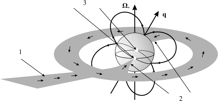
Figure 1: The scheme explaining how matter may be accreted by a compact gravitating object that has a strong pure quadrupole magnetic field. The axes of the primary star’s rotation and symmetry of the quadrupole magnetic field are shown by vectors ${{\boldsymbol{\Omega}}}_{*}$ and ${{\boldsymbol{q}}}$ respectively. The lines of the geographic and magnetic equator are shown. The numbers are corresponded to: 1 — accretion stream, 2 — accretion columns, 3 — quadrupole hot spots.

Intermediate polars have accretion disks disrupted by the magnetic field at the inner edge of the disk. Figure 1 schematically demonstrates the main features of disk accretion in a close binary system where the accretor possesses a strong purely quadrupole magnetic field. The axis of symmetry of the field (denoted by the vector ${{\boldsymbol{q}}}$) is inclined with respect to the rotation axis of the star (denoted by the vector of the angular velocity of the star’ proper rotation ${{\boldsymbol{\Omega}}}_{*}$). The matter of the accretion stream forms a ring in the immediate vicinity of the white dwarf’s surface, since the magnetic field does not allow it to fall directly onto the surface. The accreted matter has significant angular momentum. Thus, the plane of symmetry of the ring almost coincides with the orbital plane of the binary system. In the case of the quadrupole magnetic field, matter can get onto the accretor’s surface either in regions of the magnetic poles or along the magnetic equator. However, consideration of the conservation law of angular momentum, one can see that the most effective regime is when matter is accreted onto the points of intersection of the magnetic (red line) and geographic (blue line) equators of the star. Exactly at these points (yellow circles) accretion hot spots will form. We must emphasize that at these points the magnetic field has no preferred direction since the magnetic lines coming from the northern and southern magnetic poles have different directions. Hence the radiation originating in these zones will not be polarized in pure quadrupole fields, in contrast with the radiation originating in hot spots on the magnetic poles. We suggest that models of this type may be applicable to some intermediate polars, but more detailed studies covering more of the parameter space are required.

Asynchronous polars, also known as BY Cam stars (coined by Patterson [12]) offer observations that strongly constrain magnetic field configurations. This results from the fact that periodic (or quasi-periodic) variations in accretion flow geometry result as the accretion flow evolves. This is because the $L_{1}$ point originates from all azimuthal angles, with respect to the magnetic field, over the spin-orbit beat cycle. By the present time several ($\sim 4$) asynchronous polars have been confirmed. The most known representative of this subtype is the BY Cam system itself, in which the period of the proper rotation of the white dwarf differs from the orbital period by approximately $1\%$ (see e.g. [7]). There is significant evidence for a complex magnetic field from polarimetry observations [7, 13] and as such the accretion flow cannot be adequately modelled by an offset dipole field [7].

The asynchronous rotation of the white dwarf in BY Cam and the complex structure of its magnetic field result in light curves that evolve as a function spin-orbit beat phase [6, 7, 14, 15, 17]. These studies generally support the complex field model of Mason et al. [5]. Specifically, in BY Cam there is a $\sim$ 2 minute difference between the spin and orbital periods allowing for the sampling of the magnetic field structure at all phases of the 14.1 day spin-orbit beat-cycle. This is a bit like dropping iron filings all around a magnet in the classic physics demonstration, to examine field structure. Synchronized polars sample accretion flow from a single azimuthal angle. So, by calculating the accretion flow at a variety of azimuthal angles we simultaneously create models for 10 polars and a single asynchronous polar, with the spin-orbit characteristics of BY Cam. This allows for a study of polars as function of azimuthal angle. It also provides an initial attempt to model the pole switching process in BY Cam. It is hoped that further exploration of poorly constrained parameters such as accretion rate and mass ratio are needed before a proper model of BY Cam can be expected.

3D numerical simulations of mass transfer process in semi-detached binary systems without taking into account the magnetic field of the accretor star was performed in papers [18, 19, 20, 21, 22, 23, 24, 25, 26, 27]. In these works a self-consistent numerical model for gas-dynamics in close binary systems without magnetic field was first developed and the basic characteristics of the flow structure was obtained.

Recently authors [28, 29] developed a 3D parallel numerical code for simulations of the flow structure in close binary systems that takes into account the proper magnetic field of the accretor. In recent works [28, 30, 31], the code was utilized to investigate the flow structure in a close binary system (SS Cyg was taken as an example) with a relatively weak magnetic field ($10^{5}$ G on the surface) of the pure dipole type. In [32] a modification of the code was introduced. This modification allows for simulations of systems with strong dipole magnetic fields ($10^{7}$–$10^{8}$ G).

Pioneering 3-D MHD simulations of the disk-like accretion onto a star with complex geometry of the magnetic field have been performed [33, 34]. Results of these simulations showed that in the case of the disk-like accretion onto a star with a purely quadrupole magnetic field the matter of the disk is accreted in the vicinity of the quadrupole magnetic belt. If the dipole component is taken into account the belt shifts toward the southern magnetic pole since in the northern hemisphere the total magnetic field is stronger than in the southern hemisphere. Romanova et al. [35] considered more complex configurations of the magnetic field where an octupole component exists. These models were used to model the disk-like accretion onto young stars of the T Tau type.

In this paper we describe a modification of the numerical model designed to simulate systems where accretors have a complex magnetic field structure. We simulate the flow structure in polars with a complex magnetic field including aligned dipole and quadrupole components. These calculations are performed at ten different azimuthal angles thereby calculating ten separate polar models. Putting these together yields a single asynchronous polar model. We are able to see how in polars, single spot accretion may be misleading; and how accretion in asynchronous polars provide powerful constraints on magnetic field configurations.

The paper is composed as follows. In the second section we discuss the configuration of the magnetic field, describe the governing equations and the numerical method used in the frame of the modified model. In the third section results of the 3-D simulations of the flow structure are presented and possible observational indicators of flow features are discussed. In the final section the main results of the work are briefly discussed and summarized.

2 Description of the model

2.1 Magnetic field

To describe plasma flow in a close binary system it is convenient to use a non-inertial reference frame that rotates with the system having angular velocity ${{\boldsymbol{\Omega}}}$ with respect to its center of mass. In this frame we choose a Cartesian coordinate system ($x$, $y$, $z$). The origin of the coordinate system is placed at the center of the accretor and the center of the donor is placed at the distance $A$ from the accretor on the $x$-axis. The $z$ axis is directed along the rotation axis of the binary. The secondary transfers matter through the inner Lagrangian point $L_{1}$ since in this point the pressure gradient is not balanced by gravity.

Let us consider a close binary system with the accretor rotating synchronously, i.e. its rotational period is equal to the orbital one. In the absence of currents in the envelope of the binary the magnetic field will be the proper field of the accretor ${{\boldsymbol{B}}}_{*}$. The magnetic field of the accretor in the region of the magnetosphere may be rather strong. Thus the magnetic field in plasma ${{\boldsymbol{B}}}$ is conveniently treated as a superposition of the accretor’s field and the field induced by currents in the plasma: ${{\boldsymbol{B}}}={{\boldsymbol{B}}}_{*}+{{\boldsymbol{b}}}$.

This implies that in the envelope the proper magnetic field of the accretor must satisfy the condition $\nabla\times{{\boldsymbol{B}}}_{*}=0$ since it is governed by currents inside the accreting star. Thus, in the envelope this field can be described with the scalar potential: ${{\boldsymbol{B}}}_{*}=-\nabla\varphi$. The complex magnetic field of the accretor is taken to be a superposition of the multipole components of the field. Further we assume that every multipole component of the field is axisymmetric. In general the axes of symmetry of different multipole components may not be coincident. In our current model, we take into account only the dipole and quadrupole components of the magnetic field of the accretor.

The magnetic induction corresponding to the dipole component of the field is

$${{\boldsymbol{B}}}_{d}=\frac{\mu}{r^{3}}\left[3({{\boldsymbol{d}}}\cdot{{\boldsymbol{n}}}){{\boldsymbol{n}}}-{{\boldsymbol{d}}}\right],$$ (1)

where $\mu$ is the magnetic moment of the accretor, ${{\boldsymbol{d}}}$ is a unit vector that determines the axis of symmetry of the dipole field, ${{\boldsymbol{n}}}={{\boldsymbol{r}}}/r$. The vector of the magnetic moment is ${{\boldsymbol{\mu}}}=\mu{{\boldsymbol{d}}}$. Let us denote the value of the magnetic induction on the magnetic pole of the dipole field of the star as $B_{d,\text{a}}$. Then, using (1) the magnetic moment is $\mu=B_{d,\text{a}}R^{3}_{\text{a}}/2$, where $R_{\text{a}}$ is the accretor’s radius.

The potential corresponding to the quadrupole component of the field is characterized by a tensor of the quadrupole moment $D_{ik}$. If the distribution of currents inside the accretor is axisymmetric then the diagonal components of the quadrupole moment are $D_{11}=D_{22}=-D/2$, $D_{33}=D$ and all the non-diagonal components are zero. In this case the induction of the corresponding magnetic field can be described as

$${{\boldsymbol{B}}}_{q}=\frac{3D}{4r^{4}}\left[5({{\boldsymbol{q}}}\cdot{{\boldsymbol{n}}})^{2}{{\boldsymbol{n}}}-{{\boldsymbol{n}}}-2({{\boldsymbol{q}}}\cdot{{\boldsymbol{n}}}){{\boldsymbol{q}}}\right],$$ (2)

where ${{\boldsymbol{q}}}$ is a unit vector that determines the axis of symmetry of the quadrupole field. Let us denote the value of the magnetic induction on the magnetic pole of the quadrupole field of the star as $B_{q,\text{a}}$. Then, using (2) the quadrupole moment is $D=2B_{q,\text{a}}R^{4}_{\text{a}}/3$.

In our model the total magnetic field of the accretor is ${{\boldsymbol{B}}}_{*}={{\boldsymbol{B}}}_{d}+{{\boldsymbol{B}}}_{q}$. We assume that the axes of symmetry of the dipole and quadrupole fields are coincident (${{\boldsymbol{d}}}={{\boldsymbol{q}}}$). In this case in calculations it is convenient to set $B_{d,\text{a}}=\alpha_{d}B_{\text{a}}$, $B_{q,\text{a}}=\alpha_{q}B_{\text{a}}$, where $B_{\text{a}}$ is the total induction of the field on the magnetic pole of the accretor and the coefficients $\alpha_{d}$ and $\alpha_{q}$ satisfy the relation $\alpha_{d}+\alpha_{q}=1$ and determine the relative contributions of the dipole and quadrupole components into the total value of the magnetic field. In the plane of the magnetic equator ${{\boldsymbol{d}}}\cdot{{\boldsymbol{n}}}=0$, ${{\boldsymbol{q}}}\cdot{{\boldsymbol{n}}}=0$. Thus the dipole and quadrupole field inductions are:

$$B_{d}=\frac{B_{d,\text{a}}}{2}\frac{R^{3}_{\text{a}}}{r^{3}},\quad B_{q}=\frac{B_{q,\text{a}}}{2}\frac{R^{4}_{\text{a}}}{r^{4}}.$$ (3)

The ratio of these values is $B_{d}/B_{q}=(\alpha_{d}/\alpha_{q})(R_{\text{a}}/r)$. This relation demonstrates that if $\alpha_{q}>\alpha_{d}$ then in the vicinity of the magnetic equator a certain region will exist where the quadrupole field predominates over the dipole field.

Figure 2: Geometry of the accretor’s magnetic field. The gray scale of the field lines corresponds to the value of the magnetic induction $B_{*}$. The rotation axis of the accretor and the magnetic axis are shown.

The geometry of the magnetic field we use in our calculations is shown in Fig. 2. The lines with the arrows are the field lines. The gray scale of the lines corresponds to the value of the magnetic induction. The vertical line is the accretor’s rotaiton axis. The inclined line denotes the axis of symmetry of the magnetic field. The maximal value of the induction on the accretor’s surface is achieved on the magnetic poles and along the line located near the magnetic equator. For a purely quadrupole field this line coincides with the magnetic equator. If the dipole component is also taken into account this line slightly shifts southwards.

Indeed, let us denote the scalar product as ${{\boldsymbol{d}}}\cdot{{\boldsymbol{n}}}=\cos\theta$. The normal component of the magnetic field on the accretor’s surface (taking into account (1) and (2) is equal to

$${{\boldsymbol{n}}}\cdot{{\boldsymbol{B}}}_{*}=B_{\text{a}}\left(\alpha_{d}\cos\theta+\frac{3}{2}\alpha_{q}\cos^{2}\theta-\frac{3}{2}\alpha_{q}\right).$$ (4)

Calculating the derivative with respect to $\theta$ we can find values of the angle $\theta_{*}$ corresponding to maximal values of the magnetic field on the accretor’s surface. For $\theta_{*}$ we have the equation:

$$\alpha_{d}\sin\theta_{*}+3\alpha_{q}\cos\theta_{*}\sin\theta_{*}=0.$$ (5)

For a purely dipole field we have two solutions: $\theta_{*}=0$, $\pi$. They correspond to magnetic poles. For a purely quadrupole field ($\alpha_{d}=0$, $\alpha_{q}=1$) we have one more solution: $\theta_{*}=\pi/2$. This solution corresponds to the magnetic equator. Finally, in the general case we have

$$\cos\theta_{*}=-\frac{\alpha_{d}}{3\alpha_{q}}.$$ (6)

This means that if we regard both the dipole and quadrupole components the line of the strong field lies a little lower than the magnetic equator ($\theta_{*}>\pi/2$).

2.2 Basic equations

Plasma dynamics in a strong external magnetic field are characterized by the relatively slow average motion of particles along the field lines, their drift across the field lines, and propagation of very rapid Alfvén and magneto-sonic waves against a background of this slow motion. Over the characteristic dynamical time scale, the MHD waves can cross the flow region (along a column-like stream, for example) many times. Therefore, we can investigate the average flow pattern, considering the influence of the fast pulsations analogous to the MHD wave turbulence. To describe the slow motion of plasma itself, it is necessary to separate out rapidly propagating fluctuations and apply a well defined procedure for averaging over the ensemble of wave pulsations. Such a model for description of MHD flows in polars was developed in our recent work [32].

Plasma flow that occurs in a close binary system due to mass transfer can be described using the following system of modified MHD equations taking into account the strong magnetic field ${{\boldsymbol{B}}}_{*}$ of the compact object:

$${\dfrac{\partial{\rho}}{\partial{t}}}+\nabla\cdot\left(\rho{{\boldsymbol{v}}}\right)=0,$$ (7)

$${\dfrac{\partial{{{\boldsymbol{v}}}}}{\partial{t}}}+\left({{\boldsymbol{v}}}\cdot\nabla\right){{\boldsymbol{v}}}=-\dfrac{\nabla P}{\rho}-\dfrac{{{\boldsymbol{b}}}\times(\nabla\times{{\boldsymbol{b}}})}{4\pi\rho}+2({{\boldsymbol{v}}}\times{{\boldsymbol{\Omega}}})-\nabla\Phi-\dfrac{{{\boldsymbol{v}}}_{\perp}}{\tau},$$ (8)

$${\dfrac{\partial{{{\boldsymbol{b}}}}}{\partial{t}}}=\nabla\times\left[{{\boldsymbol{v}}}\times{{\boldsymbol{b}}}+{{\boldsymbol{v}}}\times{{\boldsymbol{B}}}_{*}-\eta(\nabla\times{{\boldsymbol{b}}})\right],$$ (9)

$$\rho T\left[{\dfrac{\partial{s}}{\partial{t}}}+({{\boldsymbol{v}}}\cdot\nabla)s\right]=n^{2}\left(\Gamma-\Lambda\right)+\dfrac{\eta}{4\pi}(\nabla\times{{\boldsymbol{b}}})^{2}.$$ (10)

Here $\rho$ is the density, ${{\boldsymbol{v}}}$ is the velocity, $P$ is the pressure, $s$ denotes the entropy per unit mass, $n=\rho/m_{\text{p}}$ is the concentration, $m_{\text{p}}$ is the proton mass, $\eta$ is the coefficient of the magnetic viscosity and $\Phi$ is the Roche potential. In deriving these equations we assumed the accretor’s magnetic field to be potential ($\nabla\times{{\boldsymbol{B}}}_{*}=0$) and stationary (${{\partial{{{\boldsymbol{B}}}_{*}}}/{\partial{t}}}=0$).

In the entropy equation (10) we take into account effects of radiative heating and cooling as well as matter heating due to the dissipation of currents (last term). It should be noted that the functions of radiative heating and cooling $\Gamma$ and $\Lambda$ depend on the temperature in a complicated manner (see [36, 37, 38, 39]). In our numerical model we use a linear approximation of these functions in the vicinity of the equilibrium temperature $T=11230$ K [20, 28, 29] that corresponds to the effective temperature of the accretor of $37000$ K. The term $2({{\boldsymbol{v}}}\times{{\boldsymbol{\Omega}}})$ in the equation of motion (8) describes the Coriolis force. The density, entropy and pressure are connected via the equation of state of the ideal gas: $s=c_{V}\ln(P/\rho^{\gamma})$. Here $c_{V}$ is the gas specific heat at constant volume and $\gamma=5/3$ is the adiabatic index.

The last term in the equation of motion (8) describes the force the magnetic field on the gas flow. This force influences the plasma velocity component ${{\boldsymbol{v}}}_{\perp}$ perpendicular to magnetic field lines. We note that the particles’ motion perpendicular to field lines is mainly caused by the gravity of the compact object (gravitational drift, see, e.g., [40, 41, 42]). Due to the Larmor character of the particles’ motion in the magnetic field their average motion in the perpendicular to the field direction decreases. A strong magnetic field plays the role of an effective fluid interacting with the plasma. Thus, the last term in (8) may be regarded as a force of friction occurring between the plasma and magnetic field. This term is equivalent to the friction force acting in a plasma containing different types of particles [40, 41].

In polars no accretion disk forms and the accretion stream looks like a funnel flow moving from the inner Lagrangian point $L_{1}$ toward a magnetic pole of the accretor. In this case the main effect leading to the currents’ dissipation will probably be MHD wave turbulence conditioned by the Alfvén and magneto-sonic waves propagating through the funnel accretion flow. if this is the case, the velocity of these waves is much higher than the proper velocity of the plasma flow and in some cases may even be relativistic. The coefficient of the magnetic field’s diffusion $\eta$ concerned with the MHD turbulence can be estimated using the relation

$$\eta=\dfrac{\tau_{w}}{3}\langle\delta{{\boldsymbol{v}}}^{2}\rangle,$$ (11)

where $\tau_{w}$ is the correlation time of pulsations, $\delta{{\boldsymbol{v}}}$ is the velocity fluctuations and the angle brackets mean values averaged over the wave pulsations ensemble. This relation may be parametrized as follows

$$\eta=\alpha_{w}\dfrac{B_{*}l_{w}}{\sqrt{4\pi\rho}},$$ (12)

where $\alpha_{w}$ is a dimensionless parameter close to the unity that determines the efficiency of the wave diffusion and $l_{w}$ is the specific spatial scale of the pulsations. This term may be set using the scale of inhomogeneity of the background magnetic field $l_{w}={B_{*}}/{|\nabla B_{*}|}$. In the demonstrated calculations $\alpha_{w}=0.3$. The relaxation time is taken to be $\tau=4\pi\rho\eta/B_{*}^{2}$.

2.3 Numerical method

For mCV simulations we used the 3-D parallel numerical code Nurgush [28, 29, 30, 32]. The code is based on a finite-difference Godunov type scheme of a high approximation order. An original method of unified variables for MHD [43] allowed us to use adaptive meshes in the code. In the calculation described below we used a geometrically adaptive mesh that was concentrated near the accretor’s surface. It allowed us to significantly increase the resolution of the magnetosphere region. To minimize numerical errors in the finite-difference scheme only the magnetic field induced by currents in the accretion stream and outer envelope is calculated [44, 45]. To remove the divergence of the magnetic field we use an eight-wave method [45, 46].

The equation describing the diffusion of the magnetic field was solved using an implicit locally one-dimensional method with the factorized operator [47]. It should be noted that this equation in the curvilinear non-orthogonal coordinate system, conditioned by the adaptive mesh, contains mixed spatial derivatives. To solve this problem our method use the regularization of the factorized operator. In fact, the regularization is done by substitution of the operators-multipliers constituting the initial factorized operator with certain equivalent tridiagonal operators. Hence, the regularization parameter is determined by the maximal absolute eigenvalue of the metric tensor describing the curvilinear coordinate system. The resulting system of linear algebraic equations with a tridiagonal matrix is solved numerically using the Thomas algorithm.

3 Results of simulations

3.1 Parameters

In order to explore polar accretion in the presence of a complex field as a function of azimuthal angle we consider the properties of the asynchronous polar BY Cam. In addition to providing an ensemble of ten synchronized polars, it is a first step in modelling asynchronous polars. We investigate the flow structure in an interacting binary whose parameters correspond to an asynchronous polar, with the same orbital and rotational periods as BY Cam (see, e.g., [5]). Other properties of the BY Cam binary are not well constrained and so are generally estimated here. A more detailed attempt at modelling BY Cam specifically awaits future work, since this requires confrontation with observations at each spin-orbit beat phase. Modelling an asynchronous polar, in this manner, is significantly more constraining than a synchronized polar, since the field structure at each azimuthal angle is sampled as an asynchronous polar progresses through its spin-orbit beat cycle.

The donor star (red dwarf) in our model has the mass $M_{\text{d}}=0.5\leavevmode\nobreak\ M_{\odot}$ and an effective temperature of $4000$ K. The accretor (white dwarf) has the mass $M_{\text{a}}=1\leavevmode\nobreak\ M_{\odot}$. The orbital period of the system is $P_{\text{orb}}=3.36$ hours and its semi-major axis is $A=1.3\leavevmode\nobreak\ R_{\odot}$. The inner Lagrangian point $L_{1}$ is located at the distance of $0.57\leavevmode\nobreak\ A$ from the accretor’s center. The rotational period of the accretor in BY Cam is $P_{\text{spin}}=3.32$ hours. This value differs from the value of the orbital period by approximately $1\%$. In the reference frame associated with the binary the accretor makes complete rotation in $P_{\text{beat}}=14.1$ days ($1/P_{\text{beat}}=1/P_{\text{spin}}-1/P_{\text{orb}}$) that is about 101 orbital periods. However, the actual beating and dynamics of pole switching within BY Cam is not modelled and importantly, the spin and beat periods are independent of our calculations, since we are assuming synchronous rotation for each of ten azimuthal angles. Hence, the beat phase calculations are applicable to any asynchronous polar as long as the asynchronism is no more than a few percent.

The surface magnetic induction of the white dwarf in BY Cam is estimated from observations of cyclotron humps as $28$ MG [48]. This is a very typical magnetic field strength for polars. In our model the axes of the dipole and quadrupole field are coincident. The angle of inclination of the magnetic field with respect to the axis of the accretor’s rotation is chosen to be $30^{\circ}$. In the calculations we used a value of the coefficient $\alpha_{q}=10\alpha_{d}$. This means that on the magnetic equator, the quadrupole field component is 10 times larger than the dipole component. With that, the radius of the affected zone of the quadrupole field (a distance at which values of $B_{d}$ and $B_{q}$ become equal (see (3)) may be estimated as $r=10\leavevmode\nobreak\ R_{\text{a}}$. Of course, the presence of a strong magnetic field significantly influences the process of the mass transfer in mCVs. In addition, the presence of the quadrupole component can noticeably complicate the character of the accretion of matter onto the white dwarf. Thus, information on the flow structure obtained using 3-D numerical simulations, and their confrontation with observations, will promote a deeper understanding of the physical processes involving the interaction of matter with complex magnetic fields. The results in this paper offer a start to the exploration of the vast parameter space, largely unconstrained by observations, available to polars by examining accretion flow structure as a function of azimuthal angle of the secondary with respect to the magnetic field.

The following initial and boundary conditions were utilized in our model, based on values thought typical in polars. At the inner Lagrangian point $L_{1}$ we set the gas velocity equal to the local sound speed $c_{s}=7.4\leavevmode\nobreak\ \text{km}/\text{s}$ corresponding to the donor’s effective temperature of $4000$ K. The density of gas in $L_{1}$ is $\rho(L_{1})=1.1\leavevmode\nobreak\ \times\leavevmode\nobreak\ 10^{-7}\leavevmode\nobreak\ \text{g}/\text{cm}^{3}$ and the mass transfer rate is $\dot{M}=10^{-9}\leavevmode\nobreak\ M_{\odot}/\text{yr}$. At the other boundaries of the computational domain, the following boundary conditions were set up: the density was $\rho_{\text{b}}=10^{-6}\leavevmode\nobreak\ \rho(L_{1})$; the temperature was $T_{\text{b}}=11230$ K; the velocity was ${{\boldsymbol{v}}}_{\text{b}}=0$ and the magnetic field was ${{\boldsymbol{B}}}_{\text{b}}={{\boldsymbol{B}}}_{*}$. The accretor was set up as a sphere of radius $0.0125\leavevmode\nobreak\ A$ at whose boundary the free inflow boundary condition was defined. With that, the plasma inflow vector was made parallel to the vector ${{\boldsymbol{B}}}_{*}$. All the matter having entered the cells occupied by the accretor is considered to have fallen onto the white dwarf. The initial conditions in the entire computational domain were as follows: the density was $\rho_{0}=10^{-6}\leavevmode\nobreak\ \rho(L_{1})$; the temperature was $T_{0}=11230$ K; the velocity was ${{\boldsymbol{v}}}_{0}=0$ and the magnetic field was ${{\boldsymbol{B}}}_{0}={{\boldsymbol{B}}}_{*}$. The task was solved in the computational domain of the dimension of ($-0.56A\leq x\leq 0.56A$, $-0.56A\leq y\leq 0.56A$, $-0.28A\leq z\leq 0.28A$) in the geometrically adaptive mesh [29] containing $128\leavevmode\nobreak\ \times\leavevmode\nobreak\ 128\leavevmode\nobreak\ \times\leavevmode\nobreak\ 64$ cells. The calculations presented below were performed using the computational facility of the Joint Supercomputer Center of the Russian Academy of Sciences.

Numerical experiments showed that the solution achieves the quasi-stationary regime in a specific time approximately equal to the orbital period $P_{\text{orb}}$. The criterion testifying that the solution is in the quasi-stationary regime is the condition of constancy of the entire mass of matter in the computational domain. The specific time during which the solution becomes quasi-stationary is considerably shorter than $P_{\text{beat}}$ of our model asynchronous polar,so indeed our results are applicable to asynchronous polars with beat periods of several days or more. Thus, in this work we performed simulations of the flow structure separately for different azimuthal angles of polars, but we may apply these to phases of the $P_{\text{beat}}$ period disregarding the proper rotation of the accretor. Totally we modelled ten phases corresponding to time moments $mP_{\text{beat}}$, where $m$ varied from $0$ to $0.9$ with the step of $0.1$ (this corresponds formally to ten different possible polars). The initial phase $m=0$ corresponds to the accretor’s position when the northern magnetic pole was located at the opposite from the donor side of the accretor (i.e. on the positive arm of the $x$ axis).

3.2 Flow structure

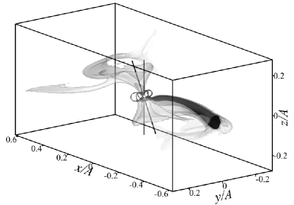
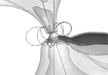
Figure 3: 3D structure for the phase $0$. The isosurfaces of the common logarithm of the density (in units of $\rho(L_{1})$) for values $-6$, $-5$ and $-4$ and the magnetic field lines are shown. The gray scale of the field lines corresponds to the value of the magnetic induction. The straight line denotes the axis of rotation of the accretor. The inclined line is the magnetic axis. In the right panel the flow structure in the vicinity of the accretor is shown.

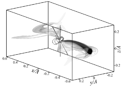
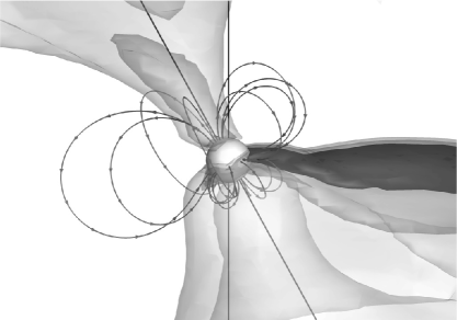
Figure 4: The same as in Fig. 3 but for the phase $0.1$.

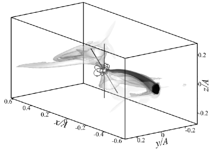
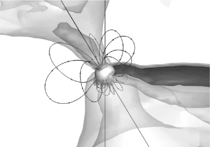
Figure 5: The same as in Fig. 3 but for the phase $0.2$.

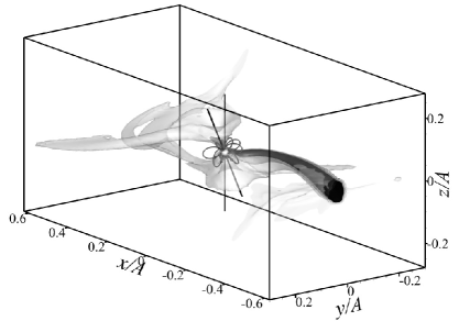
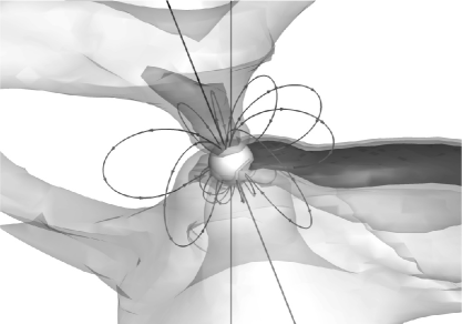
Figure 6: The same as in Fig. 3 but for the phase $0.3$.

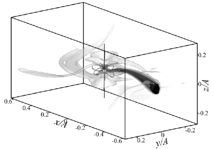
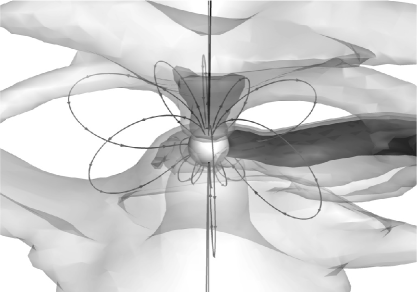
Figure 7: The same as in Fig. 3 but for the phase $0.4$.

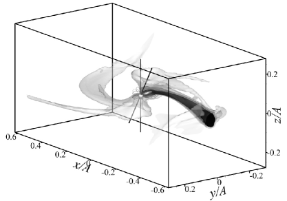
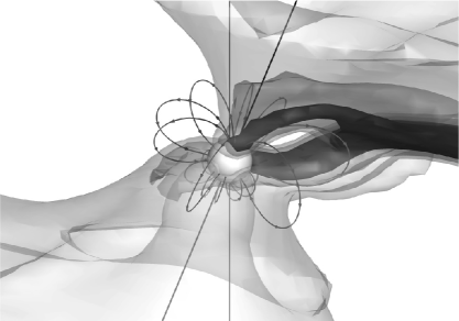
Figure 8: The same as in Fig. 3 but for the phase $0.5$.

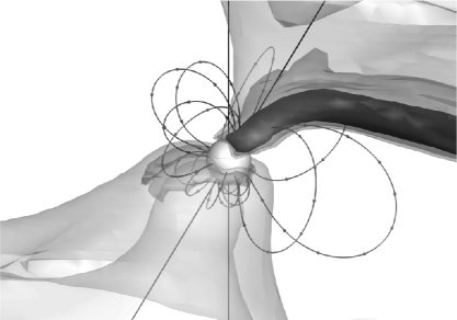
Figure 9: The same as in Fig. 3 but for the phase $0.6$.

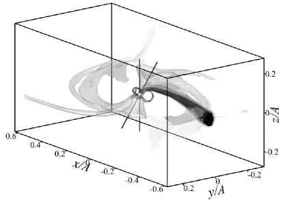
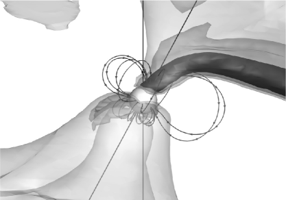
Figure 10: The same as in Fig. 3 but for the phase $0.7$.

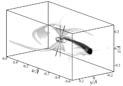
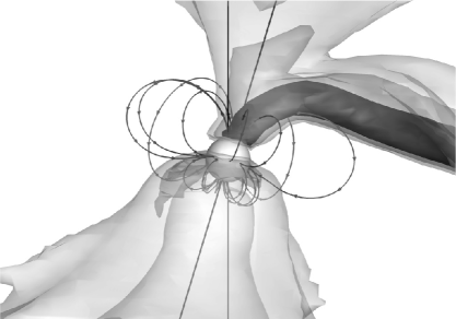
Figure 11: The same as in Fig. 3 but for the phase $0.8$.

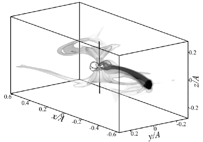
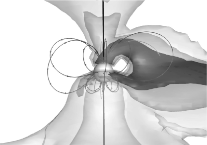
Figure 12: The same as in Fig. 3 but for the phase $0.9$.

The 3D flow structure obtained as a result of the calculations is shown in Figures 3–12. The isosurfaces of the density common logarithm (in units of $\rho(L_{1})$) for values $-6$, $-5$ and $-4$ are shown. The main stream is shown in a strongly contrasting manner. The magnetic field lines are denoted by the lines with the arrows. The gray scale of the lines corresponds to the induction of the magnetic field. The axis of the accretor’s rotation (thin straight line) and magnetic axis (bold inclined line) are also shown. The left panels demonstrate the full flow pattern in the computational domain for a given polar or asynchronous polar beat phase. The right panels illustrate the flow structure in the vicinity of the accretor.

We should note that the structure of the accretion flows in the case of complex field geometry where the quadrupole component of the field exists significantly differs from the case of a purely dipole field. Calculations performed earlier [32] showed that in close binary systems where the accretor has a strong dipole magnetic field the accretion of matter may go either onto the northern magnetic pole or the southern pole or onto both of them depending on the value of the magnetic induction and orientation of the magnetic axis. Those calculations correspond to the standard one-pole vs. two-pole accretion geometries typically applied in models involving pure dipole fields. We show from the present calculations, that other modes of accretion may exist and even be common, if a complex magnetic field is present.

Figures show that during the $P_{\text{beat}}$ period the flow structure in the system significantly changes. At phase $0$ (Fig. 3) the accretion stream emanating from the inner Lagrangian point $L_{1}$ impacts the accretor in the magnetic belt whose existence is the result of the quadrupole component of the field. This leads to formation of an accretion ring surrounding the accretor. This is in a good agreement with the scheme demonstrated above (see Fig. 1). In addition, the matter of the envelope forms an accretion stream falling onto the northern magnetic pole and a weaker stream flowing onto the southern magnetic pole. But these flows are much weaker than the main stream. Almost the same picture is seen at phases $0.1$ (Fig. 4), $0.2$ (Fig. 5) and $0.3$ (Fig.6). The structure of the accretion flows at these phases differs only by the angle between the magnetic field axis and direction to the secondary component of the binary. These calculations demonstrate that the primary accretion zone in some polars may be near the spin equator, indicating the presence of a complex field.

At phase $0.4$ (Fig. 7) the flow structure changes. The main flow of the accretion stream splits into two streams when approaching the accretor. Most of the matter still falls onto the accretor’s surface near the magnetic belt. The second flow starts to move along the field lines toward the northern magnetic pole. At phase $0.5$ (Fig. 8) this flow becomes much stronger and intensities of the two flows become nearly equivalent. Thus, at this moment two accretion zones of almost the same intensity form on the star’s surface. One of them is located at the northern magnetic pole of the star, another one lies near the magnetic belt. Some polars may be accreting in this manner. For these binaries, the presence of a complex field will be apparent.

At phases $0.6$ (Fig. 9), $0.7$ (Fig. 10) and $0.8$ (Fig. 11) the accretion flow onto the magnetic belt runs out and almost all the matter falls onto the northern magnetic pole. This flow pattern is analogous to the case of polars where the accretor possesses a purely dipole magnetic field [32].

Finally, at phase $0.9$ (Fig. 12) the second change of the flow structure during the $P_{\text{beat}}$ period occurs. The flow from the accretion stream again splits into two streams (as at the phase $0.5$). One flow still falls onto the northern magnetic pole and another forms an accretion region along the magnetic belt.

To summarize, we see that the accretion flow pattern is highly dependent on azimuthal angle. We find that among our ensemble of ten synchronized polars, single-pole accretion is most common. Often, the single-pole accretion mode occurred with flow onto a magnetic pole. This accretion mode will likely be difficult to observationally differentiate from standard dipole accretion. Another common mode found involves a single equatorial spot. The position of the equatorial spot varies somewhat as a function of azimuthal angle. In a minority of cases our model resulted in a two-pole accretion mode. In this mode, accretion takes place onto a magnetic pole and on a spot just south of the spin-equator simultaneously. The identification of such a two-pole mode would place strong constrains on magnetic field structures, such as the one modelled in this paper.

We move to the question of modelling BY Cam. It is clear that during the $P_{\text{beat}}$ period the flow structure changes twice. At those times, the accretion stream configuration and the number and location of accretion zones change. This is relatively consistent with the pole switching model of [5]. However, in that model pole switching takes place between diametrically opposed equatorial poles. It is not yet clear if the pole switching mode from a magnetic pole to an equatorial spot unveiled here may be applied to BY Cam. We expect that other system parameters, such as accretion rate, mass ratio, and magnetic field strength, not explored in the current paper will have significant affects on accretion geometry and may be modelled in the manner described here. In fact, additional accretion modes may be possible.

3.3 Hot spots

To calculate locations of hot spots forming as zones of intense accretion we used a method that was described by Romanova et al. [49]. It is assumed that when matter falls onto the accretor its thermal and kinetic energy turns into radiation. The density of the energy flux through the accretor’s surface at a given point ${{\boldsymbol{r}}}={{\boldsymbol{R}}}$ is determined by the relation:

$$f({{\boldsymbol{R}}})=-\rho{{\boldsymbol{n}}}\cdot{{\boldsymbol{v}}}\left(\varepsilon+{{{\boldsymbol{v}}}^{2}}/{2}+{P}/{\rho}\right),$$ (13)

where $\varepsilon$ is the internal energy of gas per unit mass and ${{\boldsymbol{n}}}$ is the unit vector normal to the surface. The sign ”$-$” has been chosen since on the accretor’s surface the normal component of the velocity is ${{\boldsymbol{n}}}\cdot{{\boldsymbol{v}}}<0$. As a result the value $f({{\boldsymbol{R}}})$ appears positive in (13).

For the sake of simplicity we assume that the radiation coming from the accretion zones is of the black body type. This means that the local effective temperature at a given point of the surface satisfies the relation: $f({{\boldsymbol{R}}})=\sigma T^{4}_{\text{eff}}({{\boldsymbol{R}}})$, where $\sigma$ is the Stefan-Boltzmann constant. We should note that in our work matter is accreted directly from the accretion stream but not from the disk as in [49]. Thus the normal component of the velocity over the entire surface of the accretor with good precision is equal to the free fall velocity,

$${{\boldsymbol{n}}}\cdot{{\boldsymbol{v}}}=-v_{\text{ff}}=-\sqrt{{2GM_{\text{a}}}/{R_{\text{a}}}}.$$ (14)

Therefore, the distribution of the energy flux density $f({{\boldsymbol{R}}})$ and, hence, the effective temperature $T_{\text{eff}}({{\boldsymbol{R}}})$ on the accretor’s surface will be determined by the density distribution $\rho({{\boldsymbol{R}}})$.

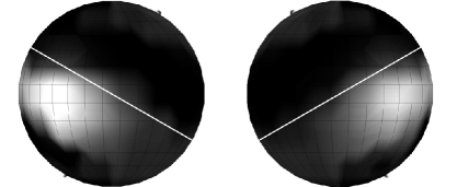
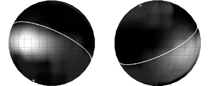
a) 0.0	b) 0.1
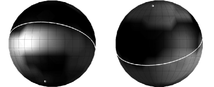
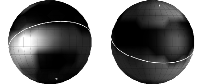
c) 0.2	d) 0.3
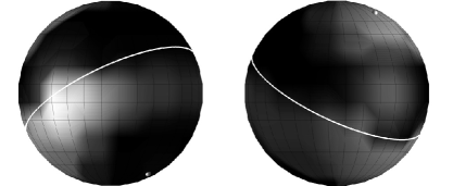
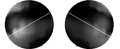
e) 0.4	f) 0.5
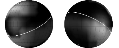
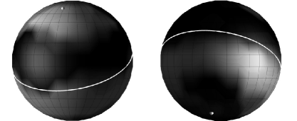
g) 0.6	h) 0.7
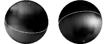
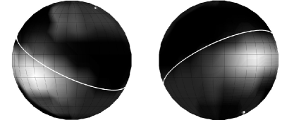
i) 0.8	j) 0.9

Figure 13: Distribution of the density common logarithm (in units of $\rho(L_{1})$) from $-8$ to $-3$ on the accretor’s surface for different phases of $P_{\text{beat}}$ period. In each diagram the left panel shows the western hemisphere, the right one shows the eastern hemisphere (see explanations in the text concerning the orientation of the coordinate system). The illuminated side of the surface faces the donor star. The line denotes the magnetic equator. The balls point to locations of the northern (upper) and southern (lower) magnetic poles.

The distribution of the radiation originating on the accretor’s surface at different azimuthal angles (phases) is shown in Fig. 13, where the distributions of the common logarithm of the accreted matter density are shown. The diagrams correspond to phases from $0$ to $0.9$ of the $P_{\text{beat}}$ period of the model asynchronous polar. The order of the diagrams is from left to right and top-down. So that the two upper diagrams (a and b) correspond to phases $0$ (left, a) and $0.1$ (right, b). The next two diagrams (second row, c and d) correspond to phases $0.2$ (left, c) and $0.3$ (right, d) etc. Finally, the two lowest diagrams (i and j) display phases $0.8$ (left, i) and $0.9$ (right, j).

In all the diagrams the same gray scale is used. The limits of the scale are $-8$ (minimal) and $-3$ (maximal). The dark (minimal density) regions correspond to the effective temperature of the white dwarf, taken to be $T_{\text{eff}}=37000$ K. The left panel of each diagram displays the western hemisphere of the star and the right one shows the eastern hemisphere. The balls in the diagrams correspond to locations of the northern (upper) and southern (lower) magnetic poles. The magnetic equator is denoted by the line.

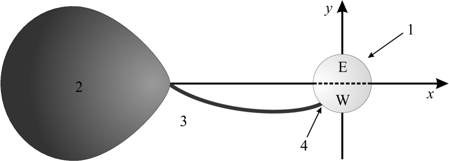
Figure 14: The scheme explaining the definition of western (W) and eastern (E) hemispheres shown on Fig. 13. The numbers are corresponded to: 1 — accretor-star, 2 — donor-star, 3 — stream, 4 — hot spot.

The images of the surface are oriented as follows (see Fig. 14). The origin of the azimuthal coordinates (longitude) is at the point located on the opposite to the donor side of the accretor. We remind the reader that in our calculations we used a Cartesian coordinate system whose origin is in the accretor and the center of the donor is at the coordinate $x=-A$. The point of intersection of the zero meridian (right edge of the left hemisphere and left edge of the right hemisphere) and the equator lies in a point with the positive $x$ coordinate. This circumstance is emphasized in the diagrams shown by the distribution of illumination of the accretor’s surface. The illuminated side faces the donor star and the shaded side is opposite.

Thus, in the diagrams, one can see density distributions on the accretor’s surface shown in a reference frame related to the donor. The coordinate frame (meridians and parallel circles) on the accretor’s surface does not describe the true geographical coordinate system, since it is related to the donor but not the accretor. In this coordinate system the accretor makes a full rotation during the $P_{\text{beat}}$ period. So its true geographical coordinate system always moves with respect to the drawn grid. Thus, everything looks as if we had observed the accretor during the $P_{\text{beat}}$ period sitting in the $L_{1}$ point or any other point resting in the coordinate system that rotates with the binary system.

Our analysis shows that the geometry of the hot spots on the accretor’s surface is rather complex. However it exactly corresponds to the description of the 3-D flow structure given in the previous section. All the diagrams demonstrate two main zones of accretion: in the vicinity of the northern magnetic pole and along the magnetic belt located a little lower than the magnetic equator. At the initial phase (upper left diagram, a) the main hot spot is located in the western hemisphere. On the opposite side in the eastern hemisphere one can see an analogous hot spot but of lower intensity. Formation of these two spots is in exact agreement with the accretion pattern shown in Fig. 1. The third spot that is also of low intensity forms on the northern magnetic pole. The similar distribution of the hot spots is observed at phases $0.1$, $0.2$ and $0.3$ (diagrams b, c and d).

As we noted above at phase $0.4$ the flow structure changes. The main accretion flow splits into two flows. As a result the hot spot near the magnetic belt becomes weaker and, oppositely, the hot spot on the northern magnetic pole becomes more intense. At phase $0.5$ (diagram f) we can see two corresponding spots of approximately the same intensity. At phases $0.6$, $0.7$ and $0.8$ the main hot spot is on the northern magnetic pole. The second spot near the magnetic belt disappears. Finally, at the phase $0.9$ (diagram j) the accretion stream splits again and forms two simultaneous hot spots.

Thus during the $P_{\text{beat}}$ period the intensity, location and number of the hot spots varies in a non-trivial manner. Equivalently, we see considerable variation in our sample of ten polars as a function of azimuthal angle. We should note that the radiation originating from the magnetic pole is significantly polarized since the magnetic field in this region has a preferential direction. At the same time the radiation of the hot spot located near the magnetic belt is not polarized since the magnetic field in this region has no preferential directions.

Figure 15: Variations of the total intensity of the radiation coming from the western and eastern hemispheres of the accretor’s surface during the $P_{\text{beat}}$ period.

In Figure 15 we show curves describing variations of the total intensity of the radiation (in arbitrary units) coming from the accretor’s surface during the $P_{\text{beat}}$ period. The solid curve corresponds to the western hemisphere and the dashed line corresponds to the eastern hemisphere. Figure shows that the radiation that of the western hemisphere is much more intense than of the eastern hemisphere. This is because the accretion stream approaches the accretor from the side of the western hemisphere due to the rotation of the binary. Thus most of the energy is released exactly in this region.

In the curve corresponding to the western hemisphere one can see two maxima and two minima. So, during the $P_{\text{beat}}$ period we see two bursts of intensity. The amplitude of the intensity variations can reach 65%. The first burst starts from the deep minimum at the phase $0.6$ and finishes at the phase $0.1$. The second burst is more sharp and approaches its maximum at the phase $0.4$. It is interesting to note that at these phases ($0.1$ and $0.4$) the maxima are observed also in the curve corresponding to the eastern hemisphere. The intensity of the radiation coming from the eastern hemisphere varies with an amplitude of up to 60%.

Comparison of the curves in Fig. 15 with the diagrams of Fig. 13 shows that the intensity maxima occur at time moments when the hot spot near the magnetic belt is located exactly on the geographical equator of the accretor. The radiation flux from the second hot spot located on the northern magnetic pole is weaker since it is on the edge of the accretor’s limb.

3.4 Synthetic light curves

To make the presentation of the simulation results and comparison of them with observations more illustrative we computed synthetic light curves. They allow one to trace and investigate variations of the intensity of the systems’s radiation concerned with variations of the location and number of the hot spots on the accretor’s surface. To compute the light curves we used the method described by Romanova et al. [49].

The intensity of the radiation originating on the accretor’s surface was calculated using the following relation:

$$I=\dfrac{1}{\pi}\int\limits_{\cos\beta>0}f({{\boldsymbol{R}}})\cos\beta\,dS,$$ (15)

where $dS$ is the element of the spherical surface, $\cos\beta={{\boldsymbol{k}}}\cdot{{\boldsymbol{n}}}$, ${{\boldsymbol{k}}}$ is the unit vector directed from the given point of the surface to the observer. The vector ${{\boldsymbol{k}}}$ is determined by the angle $i$ of the inclination of the orbital plane with respect to the picture plane: $\cos i={{\boldsymbol{\Omega}}}\cdot{{\boldsymbol{k}}}/\Omega$. The integration in (15) is performed over only the visible for the observer side of the hemisphere ($\cos\beta>0$). The absence of eclipses in this model means that the range of allowed inclination angles must be $i\lesssim 60^{\circ}$ or $i\gtrsim 120^{\circ}$.

Figure 16: Synthetic light curves computed for different phases of the $P_{\text{beat}}$ period. The different curves in the graphs correspond to different inclination angles $i$.

The resulting synthetic light curves are shown in Fig. 16. The graphs correspond to different azimuthal angles or phases of the $P_{\text{beat}}$ period. The different curves in the graphs correspond to different inclination angles $i$ of the binary.

Analysis of the light curves show that during the $P_{\text{beat}}$ period the amplitude of the radiation intensity may vary up to factor of $2$ depending on the value of the inclination, $i$. The first half of the $P_{\text{beat}}$ period is relatively quiescent since the accretor in this period faces the observer with its eastern hemisphere. Since, from the analysis there are no intense hot spots formed in the eastern hemisphere at those times. The second half of the $P_{\text{beat}}$ period is, in contrast, much more active. During these beat phases, the accretor points its western hemisphere to the secondary. The hot spots which are formed at the foot-points of the accretion stream in the western hemisphere cause an increase of the system brightness at these beat phases. Observed light curves of BY Cam [6, 7, 15, 17] demonstrate very similar behaviour, as they also very by a factor $\sim$ 2 as a function of spin-orbit beat phase.

Another interesting effect observed in the synthetic light curves is the result of shifts in positions of minima and maxima during the $P_{\text{beat}}$ period. For example, at phase $0.6$ the brightness maximum is achieved at the orbital phase $0.6$ while at spin-orbit beat phases of $0.8$ and $0.9$ it is achieved at the orbital phase $0.8$. The brightness minimum at the spin-orbit phase $0.6$ corresponds to the orbital phase $0.1$ while at spin-orbit phase $0.9$ this minimum occurs at orbital phase $0.4$. We note that similar phase shifting occurs in the observed light curves of BY Cam [6, 7, 15, 17].

This sort of phase shifting is strong circumstantial evidence for the existence of an equatorial accretion region in BY Cam, as the dipolar accretion spot does not result in significant phase shifting as a function of azimuthal angle. The results of our calculations are encouraging, but we expect that further exploration of polar parameter space may yield significant refinement of this first attempt at asynchronous polar modelling with complex magnetic fields.

4 Conclusions

In the paper we present a numerical study designed to investigate the mass transfer process in cataclysmic variables where a strong magnetic field having complex geometry exists. In our model, we suppose that the magnetic field of the accretor is a superposition of aligned dipole and quadrupole field components. The model is based on the following assumption. Namely, that plasma dynamics in the accretion stream issuing from the donor’s envelope through the inner Lagrangian point $L_{1}$ are determined by the slow average motion of matter and very rapid MHD waves propagating against a background of this slow motion. The strong background magnetic field plays the role of an effective fluid interacting with plasma. In the framework of this modified MHD, it is possible to simulate flows in close binary systems where the magnetic field on the accretor’s surface reaches values of $10^{7}$–$10^{8}$ G, corresponding to the case of polars. In the numerical model we also have taken into account processes of the diffusion of the magnetic field due to the MHD wave turbulence and processes of radiative heating and cooling.

Using a magnetic field model developed and implemented as a modified 3-D parallel numerical code, we performed simulations of the MHD flow structure in an ensemble of 10 synchronized polars. We present results of the calculations for accretion flows for ten polar orientations, with only azimuthal angle variations. The results are also applied to asynchronous polars and determined to be valid as long as the spin and orbital periods differ by at most a few percent. In the framework of the asynchronous polar model these azimuthal angles correspond to ten different phases around the $P_{\text{beat}}$ period that is determined by the period of the proper rotation of the accretor in the reference frame related to the binary system.

The basic conclusions of our work are as follows.

1. In close binary systems where the accretor’s field is strong and purely dipolar, the accretion of matter (with formation of corresponding hot spots) may impact either onto the northern magnetic pole, or the southern pole or both [32]. From an ensemble of ten synchronous polars with complex magnetic fields, it is shown that the existence of a strong quadrupole component of the magnetic field leads to significant complications of the accretion flow. The affect on the accretion flow and resulting accretion impact zones are strong functions of azimuthal angle. We find that synthetic light curves vary in shape and overall intensity as a function of azimuthal angle due to the visibility of the resulting accretion regions.

2. Accretion modes in polars with complex fields include both single-pole and two-pole configurations as in the pure dipole case. However, in the complex field case, the single-pole polar may have either a spot on the magnetic pole or alternatively, it could have an accretion region on the magnetic equator, near the orbital plane. In such cases, the observations may be mistakenly described as purely dipole magnetic field. If a strong quadrupole component of the field is present then additional accretion zones and corresponding hot spots form near the magnetic belt located a little bit south of the magnetic equator. The radiation from hot spots located on the magnetic poles is strongly polarized; since, in these zones the magnetic field has a preferential direction. At the same time the radiation of the hot spots located near the magnetic belt does not exhibit polarization since in this region no preferential direction of the field exists.

3. Analysis of the light curves computed in this work shows that at orbital phases higher than $0.5$ the intensity of the radiation sharply increases (by factor of 2 and more). This is because at these orbital phases the main accretion hot spots face the observer. In addition, positions of maxima and minima of the light curve shift during the $P_{\text{beat}}$ period of our model asynchronous polar. Similar non-trivial behaviour is also shown by observed light curves of the BY Cam system [6, 7, 15]. However, in BY Cam the working model involves pole switching between two equatorial poles, while in the present model pole switching occurs between a polar spot and an equatorial spot. More studies are needed to determine if either of these complex field models can be confidently applied to BY Cam.

There is a vast parameter space, yet to be explored, to study magnetic stream accretion. Parameters that may be varied include, the inclination angle of the magnetic axis, the ratio of intensities of the dipole and quadrupole components of the field, the accretion rate, mass-ratio etc. However, in this work we did not aim to achieve the exact correspondence of the calculation results and observations. We focused our attention on the main properties of physics of the mass transfer in complex field mCVs and possible observational signatures of complex field geometry. More precise adjustment of model parameters are expected to achieve correspondence with observational data on particular mCVs, especially asynchronous polars. Such studies are needed in order to make further progress in understanding accretion in the presence of complex magnetic fields. We conclusively find that 3-D MHD calculations simulating a stream accreting magnetic white dwarf can be used to properly model complex magnetic field structure in mCVs.

This work was supported by the Basic Research Program of the Presidium of the Russian Academy of Sciences, Russian Foundation for Basic Research (projects 09-02-00064, 11-02-00076), Federal Targeted Program ”Science and Science Education for Innovation in Russia 2009-2013”.

References

- [1] B. Warner, Cataclysmic Variable Stars (Cambridge: Cambridge Univ. Press 1995).
- [2] G.D. Schmidt, S.C. West, J. Liebert, R.F. Green, H.S. Stockman, Astrophys. J. 309, 218 (1986).
- [3] K. Wu, D.T. Wickramasinghe, ASP Conf. Ser. 29, 203 (1992).
- [4] A.D. Schwope, H.-C. Thomas, K. Beuermann, V. Burwitz, S. Jordan, R. Haefner, Astron. and Astrophys. 293, 764 (1995).
- [5] P.A. Mason, I.L. Andronov, S.V. Kolesnikov, E.P. Pavlenko, N.M. Shakovskoy, ASP Conf. Ser. 85, 496 (1995).
- [6] A. Silber, P. Szkody, D.W. Hoard, et al., Monthly Notices Roy. Astron. Soc. 290, 25 (1997).
- [7] P.A. Mason, G. Ramsay, I.L. Andronov, S.V. Kolesnikov, N.M. Shakhovskoy, E.P. Pavlenko, Monthly Notices Roy. Astron. Soc. 295, 511 (1998).
- [8] F. Euchner, S. Jordan, K. Beuermann, B.T. Gänsicke, F.V. Hessman, Astron. and Astrophys. 390, 633 (2002).
- [9] F. Euchner, K. Reinsch, S. Jordan, K. Beuermann, B.T. Gänsicke, Astron. and Astrophys. 442, 651 (2005).
- [10] F. Euchner, S. Jordan, K. Beuermann, K. Reinsch, B.T. Gänsicke, Astron. and Astropys. 451, 671 (2006).
- [11] K. Beuermann, F. Euchner, K. Reinsch, S. Jordan, B.T. Gänsicke, Astron. and Astrophys. 463, 647 (2007).
- [12] J. Patterson, Publs Astron. Soc. Pacif. 106, 209 (1994).
- [13] V. Piirola, G.V. Coyne, S.J.L. Takalo, et al., Astron. and Astrophys. 283, 163 (1994).
- [14] R. Schwarz, A.D. Schwope, A. Staude, R.A. Remillard, Astron. and Astrophys. 444, 213 (2005).
- [15] E.P. Pavlenko, M. Andreev, Ju.V. Babina, ASP Conf. Ser. 372, 537 (2007).
- [16] E.P. Pavlenko, M. Andreev, Ju.V. Babina, S. Tkachenko, ASP Conf. Ser. 362, 183 (2007).
- [17] I.L. Andronov, et al., Central European J. of Phys., 6, 385 (2008).
- [18] D.V. Bisikalo, A.A. Boyarchuk, O.A. Kuznetsov, V.M. Chechetkin, Astron. Zh. 77, 31 (2000) [Astron. Rep. 44, 26 (2000)].
- [19] D.V. Bisikalo, A.A. Boyarchuk, A.A. Kilpio, O.A. Kuznetsov, V.M. Chechetkin, Astron. Zh. 78, 707 (2001) [Astron. Rep. 45, 611 (2001)].
- [20] D.V. Bisikalo, A.A. Boyarchuk, P.V. Kaygorodov, O.A. Kuznetsov, T. Matsuda, Astron. Zh. 80, 879 (2003) [Astron. Rep. 47, 809 (2003)].
- [21] D.V. Bisikalo, A.A. Boyarchuk, P.V. Kaygorodov, O.A. Kuznetsov, T. Matsuda, Astron. Zh. 81, 494 (2004) [Astron. Rep. 48, 449 (2004)].
- [22] D.V. Bisikalo, A.A. Boyarchuk, P.V. Kaygorodov, O.A. Kuznetsov, T. Matsuda, Astron. Zh. 81, 648 (2004) [Astron. Rep. 48, 588 (2004)].
- [23] D.V. Bisikalo, P.V. Kaygorodov, A.A. Boyarchuk, O.A. Kuznetsov, Astron. Zh. 82, 788, (2005) [Astron. Rep. 49 701 (2005)].
- [24] A.Y. Sytov, P.V. Kaygorodov, D.V. Bisikalo, O.A. Kuznetsov, A.A. Boyarchuk, Astron. Zh. 84, 926, (2007) [Astron. Rep. 51, 836 (2007)].
- [25] D.V. Bisikalo, D.A. Kononov, P.V. Kaygorodov, A.G. Zhilkin, A.A. Boyarchuk, Astron Zh. 85, 356 (2008) [Astron. Rep. 52, 318 (2008)].
- [26] A.Y. Sytov, D.V. Bisikalo, P.V. Kaygorodov, A.A. Boyarchuk, Astron. Zh. 86, 250 (2009) [Astron. Rep. 53, 223 (2009)].
- [27] A.Y. Sytov, D.V. Bisikalo, P.V. Kaygorodov, A.A. Boyarchuk, Astron. Zh. 86, 468 (2009) [Astron. Rep. 53, 428 (2009)].
- [28] A.G. Zhilkin, D.V. Bisikalo, Astron. Zh. 86, 475 (2009) [Astron. Rep. 53, 436 (2009)].
- [29] A.G. Zhilkin, Matem. Modelir. 22, 110 (2010).
- [30] A.G. Zhilkin, D.V. Bisikalo, Advances in Space Research 45, 437 (2010).
- [31] A.G. Zhilkin, D.V. Bisikalo, Astron. Zh. 87, 913 (2010) [Astron. Rep. 54, 840 (2010)].
- [32] A.G. Zhilkin, D.V. Bisikalo, Astron. Zh. 87, 1155 (2010) [Astron. Rep. 54, 1063 (2010)].
- [33] M. Long, M.M. Romanova, R.V.E. Lovelace, Monthly Notices Roy. Astron. Soc. 374, 436 (2007).
- [34] M. Long, M.M. Romanova, R.V.E. Lovelace, Monthly Notices Roy. Astron. Soc. 386, 1274 (2008).
- [35] M.M. Romanova, M. Long, F.K. Lamb, A.K. Kulkarni, J.-F. Donati, Monthly Notices Roy. Astron. Soc. 411, 915 (2011).
- [36] D.P. Cox, E. Daltabuit, Astrophys. J. 167, 113 (1971).
- [37] A. Dalgarno, R.A. McCray, ARA&A, 375 (1972).
- [38] J.C. Raymond, D.P. Cox, B.W. Smith, Astrophys. J. 204, 290 (1976).
- [39] L. Spitzer, Physical Processes in the Interstellar Medium (Wiley, New York, 1978; Mir, Moscow, 1981).
- [40] D.A. Frank-Kamenetskii, Lectures on Plasma Physics (Atomizdat, Moscow, 1968) [in Russian].
- [41] F. Chen, Introduction to Plasma Physics (Springer, New York, 1995; Mir, Moscow, 1987).
- [42] B.A. Trubnikov, Plasma Theory (Energoatomizdat, Moscow, 1996) [in Russian].
- [43] A.G. Zhilkin, Zh. Vychisl. Mat. Mat. Fiz. 47, 1898 (2007) [Comput. Math. Math. Phys. 47, 1819 (2007)].
- [44] T. Tanaka, J. Comp. Phys. 111, 381 (1994).
- [45] K.G. Powell, P.L. Roe, T.J. Linde, T.I. Gombosi, D.L. De Zeeuw, J. Comp. Phys. 154, 284 (1999).
- [46] P.J. Dellar, J. Comp. Phys., 172, 392 (2001).
- [47] A.A. Samarskii, The Theory of Differential Schemes (Nauka, Moscow, 1989; Marcel Dekker, New York, 2001).
- [48] A.D. Schwope, PhD. Thesis, Berlin Univ (1991).
- [49] M.M. Romanova, G.V. Ustyugova, A.V. Koldoba, R.V.E. Lovelace, Astrophys. J. 610, 920 (2004).