A perturbative probabilistic approach to quantum many-body systems

Abstract

In the probabilistic approach to quantum many-body systems, the ground-state energy is the solution of a nonlinear scalar equation written either as a cumulant expansion or as an expectation with respect to a probability distribution of the potential and hopping (amplitude and phase) values recorded during an infinitely lengthy evolution. We introduce a perturbative expansion of this probability distribution which conserves, at any order, a multinomial-like structure, typical of uncorrelated systems, but includes, order by order, the statistical correlations provided by the cumulant expansion. The proposed perturbative scheme is successfully tested in the case of pseudo-spin 1/2 hard-core boson Hubbard models also when affected by a phase problem due to an applied magnetic field.

1 Introduction

A multitude of evolution problems, including quantum many-body systems, can be cast in the form of a linear flow, namely a system of linear differential equations with respect to a parameter, the time, which can be real or imaginary. The solution of a linear flow, with a real or an imaginary time, admits an exact probabilistic representation, namely a Feynman-Kac–like formula, in terms of a proper collection of independent Poisson processes [1, 2, 3, 4, 5]. For a lattice system, the Poisson processes are associated with the links of the lattice and the probabilistic representation leads to an optimal algorithm [3, 4, 5] which coincides with the Green function quantum Monte Carlo method in the limit when the latter becomes exact [6]. The algorithm can be rigorously generalized [7] to include fluctuation control techniques, like reconfigurations and importance sampling, and allows the exact simulation of time-dependent correlation functions for system not affected by the so called sign problem [8].

In the limit of an infinitely long imaginary time, the above exact probabilistic representation has been developed to yield semi-analytical results. In fact, for an arbitrary many-body system we are able to relate the energy of its ground state to the unique solution of a nonlinear scalar equation [9, 10, 11, 12]. This equation can be written in terms of a series involving the cumulants of integers, the multiplicities $N_{V}$, $N_{T}$ and $N_{\lambda}$, which count how many times the potential, hopping and phase variables take the values $V$, $T$ and $\lambda$ during an infinitely long evolution of the system. The potential variables are, in some chosen base, the diagonal matrix elements of the Hamiltonian of the system, whereas the hopping and phase variables are related to the amplitude and phase of the off-diagonal matrix elements. Alternatively, the equation for the ground-state energy can be written in terms of an expectation involving the probability distribution of the multiplicities $N_{V}$, $N_{T}$ and $N_{\lambda}$.

The two ways of writing the equation for $E_{0}$, cumulant expansion or probabilistic expectation, correspond to two different approaches to evaluate the ground state of a many-body system. In the former case, we can imagine measuring the exact cumulants of the system up to some finite (small) order, inserting them in a corresponding truncated equation and solving it obtaining an approximation to $E_{0}$ [11]. In the latter case, we have the possibility to make some guess on the probability distribution of the multiplicities $N_{V}$, $N_{T}$ and $N_{\lambda}$ bypassing the microscopic connection between configurations of the system and values of the variables $V$, $T$ and $\lambda$. The simplest guess is to neglect any correlation among the multiplicities and assume that they are multinomially distributed. There is a class of systems for which, in the thermodynamic limit, a multinomial distribution exactly applies. The class includes the uniformly fully connected models, namely a collection of states all connected with equal hopping coefficients and in the presence of a potential operator with arbitrary levels and degeneracies, and the random potential systems, in which the hopping operator is generic and arbitrary potential levels are assigned randomly to the states with arbitrary probabilities. For this class of models we have found a zero-temperature universal thermodynamic limit displaying a quantum phase transition [12].

Both the two approaches described above have limitations. The more severe drawback of the cumulant expansion is that truncating the series corresponds to introducing a rather artificial equivalent system with zero cumulants of large order. Since the determination of $E_{0}$ is a problem which involves large fluctuations [9], we expect, and find indeed, some nonphysical behavior of the solutions corresponding to large interaction energies. On the other hand, we expect that the multinomial probability distribution used in the second approach may give quantitatively inaccurate results for most of the systems, i.e. when the correlations among the potential, hopping and phase multiplicities cannot be neglected.

In the present paper we introduce a perturbative scheme merging the merits of the cumulant expansion with those of the expectation taken from an uncorrelated multinomial distribution. The idea is to develop a perturbative expansion of the probability distribution of the multiplicities $N_{V}$, $N_{T}$ and $N_{\lambda}$ which conserves, at any order, a multinomial-like structure. Order by order, we add correlations among the multiplicities in such a way as to modify the cumulants of the multinomial-like distribution and make them to coincide with those measured in the system up to the order considered. As a result, we gain better and better approximations to the real probability distribution. At the first order, we have a probability distribution which contain infinitely many cumulants and the first one is exact; at the second order, we have a probability distribution with infinitely many cumulants and the first two are exact; and so on. In this way, we expect to obtain, even at very small perturbative orders, accurate results for the ground-state energy of both weakly- and strongly-interacting many-body systems. We have checked our perturbative scheme in the case of pseudo-spin 1/2 hard core boson Hubbard models in one- and two-dimensional lattices. In particular, we have considered the case of a ring threaded by a magnetic flux, a model which is affected by a phase problem. It is remarkable that, already at the second perturbative order, we find a ground-state energy which compares rather well with the exact value of $E_{0}$.

The main advantage of our method lies in its semi-analytical character. Once all the cumulants up to some order $k$ are measured, via a una tantum simulation, the perturbative probabilistic distribution built from these input data provides, within an approximation with improves with $k$, the ground state energy $E_{0}$ as a function of the Hamiltonian parameters (e.g. interaction and hopping amplitudes). In contrast, in a standard Monte Carlo method any different choice of the Hamiltonian parameters requires a distinct simulation. Furthermore, the cumulants are easily measured also in the case of fermions (bosons in the presence of magnetic fields). The sign (phase) problem that occurs in this case remains confined in the expression of the perturbative probability distribution and can, in principle, be addressed analytically.

There is another useful result provided by the semi-analytical character of our approach. Assuming a Hamiltonian $\hat{H}(\xi)$ function of the parameter $\xi$, we are able to evaluate the derivatives of the ground-state energy $E_{0}(\xi)$ with respect to $\xi$. This allows the determination of arbitrary ground-state correlation functions via the Hellman-Feynman theorem

$$\frac{\partial E_{0}(\xi)}{\partial\xi}=\langle E_{0}(\xi),\frac{\partial\hat{H}(\xi)}{\partial\xi}E_{0}(\xi)\rangle,$$

where we have assumed a normalized ground state $\langle E_{0}(\xi),E_{0}(\xi)\rangle=1$. In fact, the quantum expectation of an arbitrary observable $\hat{O}$ in the ground state of the Hamiltonian $\hat{H}$ can be obtained by evaluating the ground-state energy $E_{0}(\xi)$ of the Hamiltonian $\hat{H}(\xi)=\hat{H}+\xi\hat{O}$ and taking the derivative $\left.\partial_{\xi}E_{0}(\xi)\right|_{\xi=0}$.

The paper is organized as follows. In section 2 we review the probabilistic approach to quantum many-body systems. The equation for the ground-state energy is written as an expansion over the cumulants of the potential, hopping and phase multiplicities in section 2.1 and as an expectation with respect to the probability distribution of the same variables in section 2.2. In the latter section the case of an uncorrelated multinomial distribution is described in detail. In section 3 we introduce the probabilistic perturbative scheme bringing together the merits of the multinomial probability distribution with the statistical details provided by the cumulant expansion. The parameters defining the perturbative probability distribution of the potential, hopping and phase multiplicities are explicitly discussed, up to the third order, in sections 3.1 to 3.5. This is a technical part which could be skipped in a first reading. Some considerations on the higher perturbative orders are given in section 3.6. The equation for the evaluation of $E_{0}$ resulting from the above perturbative scheme is discussed in section 4. Sections 5 and 6 deal with some numerical results. In particular, in section 6 we discuss how the determination of the ground-state energy in the presence of a phase problem is handled by our approach. Concluding remarks are drawn in section 7. Two appendices close the paper. In A we review the methods for solving the nonsymmetric algebraic Riccati equation which appears in determining the perturbative parameters at the second order. B summarizes the evaluation of the perturbative parameters at the fourth order.

2 Probabilistic approach to quantum many-body systems

In this section we review the probabilistic approach to quantum many-body systems developed in [9, 10, 11, 12]. Consider a system of particles represented by a Hamiltonian operator $\hat{H}$ acting on a $M$ dimensional space of states labeled by configuration indices $\bm{n}$. As an example, think about spinless particles undergoing a simple exclusion dynamics in a lattice with configurations given by the site occupations $\bm{n}=(0,1,1,1,0,0,1,\dots)$. In the chosen $\bm{n}$-representation, we separate, as usual, $\hat{H}=\hat{K}+\hat{V}$, where $\hat{V}=\mathrm{diag}(\hat{H})$ is called the potential operator and has non vanishing matrix elements

$$V_{\bm{n},\bm{n}}=V_{\bm{n}}.$$ (1)

The hopping operator $\hat{K}$ is defined by the matrix elements

$$K_{\bm{n},\bm{n}^{\prime}}=-\lambda_{\bm{n},\bm{n}^{\prime}}~{}\eta_{\bm{n},\bm{n}^{\prime}},\qquad\eta_{\bm{n},\bm{n}^{\prime}}>0,\qquad|\lambda_{\bm{n},\bm{n}^{\prime}}|=0,1,$$ (2)

conventionally written in terms of links $\lambda_{\bm{n},\bm{n}^{\prime}}$ and positive strengths $\eta_{\bm{n},\bm{n}^{\prime}}$. The matrix with elements $|\lambda_{\bm{n},\bm{n}^{\prime}}|$ forms the so called adjacency matrix and establishes whether two configurations $\bm{n}$ and $\bm{n}^{\prime}$ are first neighbors with respect to $\hat{K}$ or not. The phase change (sign in the case of fermions) registered by connecting two first neighbor configurations $\bm{n}$ and $\bm{n}^{\prime}$ is given by $\mathop{\rm Arg}{\lambda_{\bm{n},\bm{n}^{\prime}}}$. Note that $\sum_{\bm{n}^{\prime}}|\lambda_{\bm{n},\bm{n}^{\prime}}|$ is the number of configurations which may be connected to the configuration $\bm{n}$.

The evolution of the system from an initial state $\psi_{0}$ is earned by solving the Schrödinger equation. After a time $t$ the system is found in the state $\psi(t)$ which in the chosen $\bm{n}$-representation has components (we put $\hbar=1$)

$$\langle\bm{n},\psi(t)\rangle=\sum_{\bm{n}_{0}}\langle\bm{n},\mathrm{e}^{-\mathrm{i}\hat{H}t}\bm{n}_{0}\rangle\langle\bm{n}_{0},\psi_{0}\rangle.$$ (3)

This evolution, in the same way as for any linear flow, admits an exact probabilistic representation [1, 2, 3, 4, 5]. In a one-to-one correspondence with the links, we introduce $M^{2}$ independent Poisson processes $\{N^{t}_{\bm{n},\bm{n}^{\prime}}\}$ with rates $\{\rho_{\bm{n},\bm{n}^{\prime}}\}$. We recall that for these processes the probability to jump $k$ times in the time interval $[t,t+s)$ is [13]

$$\mathrm{prob}(N^{t+s}_{\bm{n},\bm{n}^{\prime}}-N^{t}_{\bm{n},\bm{n}^{\prime}}=k)=\frac{(\rho_{\bm{n},\bm{n}^{\prime}}s)^{k}}{k!}e^{-\rho_{\bm{n},\bm{n}^{\prime}}s},\qquad k=0,1,2,\dots.$$ (4)

We establish that each time a Poisson process $N^{t}_{\bm{n},\bm{n}^{\prime}}$ jumps, the configuration of the system changes from $\bm{n}$ to $\bm{n}^{\prime}$ if $|\lambda_{\bm{n},\bm{n}^{\prime}}|=1$, otherwise it remains $\bm{n}$. Arranging the jumps according to the times, $s_{1}<s_{2}<\dots<s_{N_{t}}<t<s_{N_{t}+1}$, at which they take place in the interval $[0,t)$ we define a random walk in the configuration space of the system $\bm{n}_{0}\to\bm{n}_{1}\to\bm{n}_{2}\to\dots\to\bm{n}_{N_{t}}$ generated by the above rule from a chosen initial configuration $\bm{n}_{0}$, see figure 1. It is simple to prove that the fundamental matrix elements of the evolution operator $\langle\bm{n},\mathrm{e}^{-\mathrm{i}\hat{H}t}\bm{n}_{0}\rangle$ can be written as an expectation over the above $M^{2}$ independent Poisson processes

$$\langle\bm{n},\mathrm{e}^{-\mathrm{i}\hat{H}t}\bm{n}_{0}\rangle=\mbox{$\mathsf{E}$}\left(\delta_{\bm{n},\bm{n}_{N_{t}}}{\cal M}^{t}_{\bm{n}_{0}}\right),$$ (5)

$${\cal M}^{t}_{\bm{n}_{0}}=\mathrm{e}^{\sum_{\bm{n},\bm{n}^{\prime}}\rho_{\bm{n},\bm{n}^{\prime}}t}\left(\prod_{k=1}^{N_{t}}\mathrm{i}\lambda_{k}\eta_{k}\rho_{k}^{-1}\mathrm{e}^{-\mathrm{i}V_{k-1}(s_{k}-s_{k-1})}\right)\mathrm{e}^{-\mathrm{i}V_{N_{t}}(t-s_{N_{t}})},$$ (6)

where we put $s_{0}=0$ and introduced the shorthand

$$V_{k}=V_{\bm{n}_{k}},\qquad k=0,1,\dots,N_{t},$$ (7)

$$\lambda_{k}=\lambda_{\bm{n}_{k-1},\bm{n}_{k}},\qquad k=1,\dots,N_{t},$$ (8)

$$\eta_{k}=\eta_{\bm{n}_{k-1},\bm{n}_{k}},\quad\rho_{k}=\rho_{\bm{n}_{k-1},\bm{n}_{k}},\qquad k=1,\dots,N_{t}.$$ (9)

The rates $\{\rho_{\bm{n},\bm{n}^{\prime}}\}$ of the Poisson processes are completely arbitrary, in fact it is easy to check that $\mbox{$\mathsf{E}$}(\mathrm{d}{\cal M}^{t}_{\bm{n}_{0}}/\mathrm{d}{\rho_{\bm{n},\bm{n}^{\prime}}})=0$. Here, for simplicity, we take $\rho_{\bm{n},\bm{n}^{\prime}}=\rho$ uniform, whereas other choices, e.g. $\rho_{\bm{n},\bm{n}^{\prime}}=\eta_{\bm{n},\bm{n}^{\prime}}$, allow to define optimal Monte Carlo numerical algorithms [3, 7]. The above probabilistic representation holds also for non-autonomous systems with a time dependent potential $V_{\bm{n}}(t)$. In this case the time-ordered quantum evolution operator $\mathsf{T}\exp(-\mathrm{i}\int_{0}^{t}\hat{H}(u)\mathrm{d}{u})$ has matrix elements given by (5-6) with $V_{k}\to\int_{s_{k}}^{s_{k+1}}V_{k}(u)\mathrm{d}{u}$. The representation holds also at imaginary times $t\to-\mathrm{i}t$ with the substitutions $\lambda_{k}\to-\mathrm{i}\lambda_{k}$ and $V_{k}\to-\mathrm{i}V_{k}$.

Figure 1: Random walk with $N_{t}$ jumps in the time interval $[0,t)$: scheme of the visited configurations and of the corresponding jump times.

A convenient way to study the properties of the ground state of a particle system is to consider its evolution for a long imaginary time. Starting from an arbitrary configuration $\bm{n}_{0}$ the system finally relaxes into the ground state, assumed not to be orthogonal to $\bm{n}_{0}$. In this way we can evaluate any ground-state correlation function via time asymptotic probabilistic expressions. For instance, the ground state energy $E_{0}$ is given by

$$E_{0}=\lim_{t\to\infty}-\partial_{t}\log\sum_{\bm{n}}\langle\bm{n},\mathrm{e}^{-\hat{H}t}\bm{n}_{0}\rangle=\lim_{t\to\infty}-\partial_{t}\log\mbox{$\mathsf{E}$}(\mathcal{M}_{\bm{n}_{0}}^{t}),$$ (10)

where $\mathcal{M}_{\bm{n}_{0}}^{t}$ is the imaginary time variant of (6). It is of fundamental importance that for the expectation $\mbox{$\mathsf{E}$}(\mathcal{M}_{\bm{n}_{0}}^{t})$ we can find, at large times, an analytical result. In the following we outline how this is obtained.

First, we decompose $\mbox{$\mathsf{E}$}(\mathcal{M}_{\bm{n}_{0}}^{t})$ in a series of canonical expectations over random walks with a fixed number of jumps

$$\mbox{$\mathsf{E}$}\left({\cal M}^{t}_{\bm{n}_{0}}\right)=\sum_{N=0}^{\infty}\mbox{$\mathsf{E}$}\left({\cal M}^{t}_{\bm{n}_{0}},N_{t}=N\right)$$ (11)

and evaluate each term of this series by integrating over all possible jump times. The probability to have $N$ Poisson processes jumping in the interval $[0,t)$ with the $k$th process jumping in the interval $[s_{k},s_{k}+\mathrm{d}{s_{k}})$ amounts to

$$\prod_{k=1}^{N}\mathrm{e}^{-\sum_{\bm{n},\bm{n}^{\prime}}\rho_{\bm{n},\bm{n}^{\prime}}(s_{k}-s_{k-1})}\rho_{k}\mathrm{d}{s_{k}}.$$ (12)

With a simple calculation we then obtain

$$\mbox{$\mathsf{E}$}\left({\cal M}^{t}_{\bm{n}_{0}},N_{t}=N\right)=\sum_{r\in\Omega_{N}}\mathcal{W}_{N}^{(r)}(t)\prod_{k=1}^{N}\lambda_{k}^{(r)}\eta_{k}^{(r)},$$ (13)

where $\Omega_{N}=\Omega_{N}(\bm{n}_{0})$ is the set of all possible random walks with $N$ jumps branching from $\bm{n}_{0}$. The contribution of the $r$th random walk $\bm{n}_{0}\to\bm{n}_{1}^{(r)}\to\dots\to\bm{n}_{N}^{(r)}$ includes the factor $\mathcal{W}_{N}^{(r)}(t)=\mathcal{L}^{-1}[\tilde{\mathcal{W}}_{N}^{(r)}(z)](t)$, namely the inverse Laplace transform of

$$\tilde{\mathcal{W}}_{N}^{(r)}(z)=\prod_{k=0}^{N}\frac{1}{z+V_{k}^{(r)}}.$$ (14)

From equation (13) it is evident that only the random walks with $|\lambda_{k}^{(r)}|=1$, i.e. $\bm{n}_{k-1}^{(r)}\neq\bm{n}_{k}^{(r)}$, for $k=1,\dots,N$, contribute to the sum. Thus we can rewrite the sum over $\Omega_{N}$ as a probabilistic expectation over these effective random walks. According to the choice $\rho_{\bm{n},\bm{n}^{\prime}}=\rho$ uniform, the effective random walks correspond to a Markov chain with transition matrix $P_{\bm{n},\bm{n}^{\prime}}=|\lambda_{\bm{n},\bm{n}^{\prime}}|/\sum_{\bm{n}^{\prime\prime}}|\lambda_{\bm{n},\bm{n}^{\prime\prime}}|$ [14]. The probability that we must associate with the $r$th element of the set $\Omega_{N}$ is, therefore,

$$p_{N}^{(r)}=\prod_{k=1}^{N}\frac{|\lambda_{\bm{n}_{k-1}^{(r)},\bm{n}_{k}^{(r)}}|}{\sum_{\bm{n}}|\lambda_{\bm{n}_{k-1}^{(r)},\bm{n}}|}.$$ (15)

Note that $p_{N}^{(r)}=0$ for non effective random walks and $\sum_{r\in\Omega_{N}}p_{N}^{(r)}=1$. Multiplying and dividing each addend of equation (13) by $p_{N}^{(r)}$, we rewrite the canonical expectations as

$$\mbox{$\mathsf{E}$}\left({\cal M}^{t}_{\bm{n}_{0}},N_{t}=N\right)=\sum_{r\in\Omega_{N}}p_{N}^{(r)}\mathcal{L}^{-1}\left[\prod_{k=0}^{N}\frac{1}{z+V_{k}^{(r)}}\right](t)\prod_{k=1}^{N}T_{k}^{(r)}\prod_{k=1}^{N}\lambda_{k}^{(r)},$$ (16)

where

$$T_{k}=\eta_{\bm{n}_{k-1},\bm{n}_{k}}\sum_{\bm{n}}|\lambda_{\bm{n}_{k-1},\bm{n}}|,\qquad k=1,\dots,N.$$ (17)

Equation (16) shows that $\mbox{$\mathsf{E}$}\left({\cal M}^{t}_{\bm{n}_{0}},N_{t}=N\right)$ is the average of a quantity which does not rely on the detailed sequence of the configurations visited during the time $t$. It depends just on the multiplicities, or numbers of occurrences, of the potential, hopping and phase variables, $V$, $T$ and $\lambda$, defined by (7), (17) and (8), respectively. For a random walk with $N$ jumps, these multiplicities are explicitly defined as

$$N_{V} =\sum_{k=0}^{N}\delta_{V,V_{k}},\qquad V\in\mathscr{V},$$ (18)

$$N_{T} =\sum_{k=1}^{N}\delta_{T,T_{k}},\qquad T\in\mathscr{T},$$ (19)

$$N_{\lambda} =\sum_{k=1}^{N}\delta_{\lambda,\lambda_{k}},\qquad\lambda\in\mathscr{L},$$ (20)

where $\mathscr{V}$, $\mathscr{T}$ and $\mathscr{L}$ are the sets of all possible values assumed by (7), (17) and (8) during a random walk with infinitely many jumps. Note that $0\notin\mathscr{L}$ as jumps between configurations $\bm{n}$ and $\bm{n}^{\prime}$ with $\lambda_{\bm{n},\bm{n}^{\prime}}=0$ have zero probability to be realized. Since any configuration can be obtained from any other one by a finite number of jumps, i.e. the Markov chain we are considering is irreducible, the elements in the sets $\mathscr{V}$, $\mathscr{T}$ and $\mathscr{L}$ do not depend on the initial configuration $\bm{n}_{0}$. Let us indicate the multiplicities $N_{V}$, $N_{T}$ and $N_{\lambda}$ collectively by a vector with as many components as the elements in the set $\mathscr{H}=\mathscr{V}\cup\mathscr{T}\cup\mathscr{L}$,

$$\bm{\mu}^{\mathrm{T}}=(\ldots N_{V}\ldots;\ldots N_{T}\ldots;\ldots N_{\lambda}\ldots).$$ (21)

If we split the set $\Omega_{N}$ into subsets of random walks with equal values of $\bm{\mu}$, we conclude that

$$\mbox{$\mathsf{E}$}\left({\cal M}^{t}_{\bm{n}_{0}},N_{t}=N\right)=\sum_{\bm{\mu}}\mathcal{P}_{N}(\bm{\mu})~{}\mathcal{L}^{-1}\left[\prod_{V\in\mathscr{V}}(z+V)^{-N_{V}}\right](t)\prod_{T\in\mathscr{T}}T^{N_{T}}\prod_{\lambda\in\mathscr{L}}{\lambda}^{N_{\lambda}},$$ (22)

where

$$\mathcal{P}_{N}(\bm{\mu})=\sum_{r\in\Omega_{N}}\left(\prod_{k=1}^{N}\frac{|\lambda_{\bm{n}_{k-1}^{(r)},\bm{n}_{k}^{(r)}}|}{\sum_{\bm{n}}|\lambda_{\bm{n}_{k-1}^{(r)},\bm{n}}|}\right)~{}\delta_{\bm{\mu}^{(r)},\bm{\mu}}$$ (23)

is the probability to have random walks with multiplicities $\bm{\mu}$ after $N$ jumps from the configuration $\bm{n}_{0}$. Note that $\mathcal{P}_{N}(\bm{\mu})=0$ unless $\bm{\mu}$ satisfies the following three constraints

$$\sum_{V\in\mathscr{V}}N_{V}=N+1,\qquad\sum_{T\in\mathscr{T}}N_{T}=N,\qquad\sum_{\lambda\in\mathscr{L}}N_{\lambda}=N.$$ (24)

As a second step, we observe that when the imaginary time $t$ becomes large the full expectation (11) takes exponentially leading contributions from terms with $N\sim t$. Thus, we can replace all previous results with their $N\to\infty$ asymptotic expressions. Due to the ergodicity of the underlying Markov chain, the probability (23) looses memory of the initial configuration $\bm{n}_{0}$. We can evaluate the inverse Laplace transform which appears in (22) by a saddle point technique in the complex plane. In the same equation we can also substitute the sum over the multiplicities by an integral over $\bm{\mu}$ and avoid distinguishing the normalizations $N$ and $N+1$ in (24). As a final result we have the following asymptotic logarithm equality

$$\mbox{$\mathsf{E}$}\left({\cal M}^{t}_{\bm{n}_{0}},N_{t}=N\right)\simeq\int\mathrm{d}{(N\bm{\nu})}~{}\mathcal{P}_{N}(N\bm{\nu})~{}\frac{\mathrm{e}^{x_{0}t+N\left(\bm{\nu},\bm{u}\right)}}{\sqrt{2\pi N(\bm{\nu},\bm{w})}},$$ (25)

where we have introduced the frequencies $\bm{\nu}=\bm{\mu}/N$, which have a finite limit for $N\to\infty$, the vectors

$$\bm{u}^{\mathrm{T}} = (\ldots-\log(x_{0}+V)\ldots;\ldots\log T\ldots;\ldots\log\lambda\ldots),$$ (26)

$$\bm{w}^{\mathrm{T}} = (\ldots(x_{0}+V)^{-2}\ldots;\ldots 0\ldots;\ldots 0\ldots),$$ (27)

and the scalar product $(\bm{a},\bm{b})=\sum_{\alpha\in\mathscr{H}}a_{\alpha}b_{\alpha}$. The quantity $x_{0}$, which is the real saddle-point in the complex contour used to evaluate the Laplace antitransform, is the unique solution of the scalar equation

$$\sum_{V\in\mathscr{V}}\frac{\nu_{V}}{x_{0}+V}=\frac{t}{N},\qquad x_{0}>-V_{\mathrm{min}}.$$ (28)

Note that this equation has a regular scaling behavior for $t,N\to\infty$ with $N\sim t$.

The integral over the frequencies $\bm{\nu}$ in equation (25) is easily performed by a saddle-point method whenever the asymptotic probability density $\mathcal{P}_{N}(N\bm{\nu})$ is known. We cannot hope to evaluate this probability from the microscopic definition (23) except for very particular models. For general systems, two different strategies have been considered, see [11] and [12]. We can relate $\mathcal{P}_{N}(N\bm{\nu})$ to proper statistical moments of the system under consideration, measure or calculate some of these moments and, lastly, obtain partial information about $E_{0}$. Or we can postulate some expressions for $\mathcal{P}_{N}(N\bm{\nu})$ and see which kind of systems are described, exactly or approximately, by this guess.

2.1 Cumulant expansion

If we rewrite the probability density $\mathcal{P}_{N}(N\bm{\nu})$ in terms of its Fourier transform ${\tilde{\mathcal{P}}}_{N}(\bm{q})$

$$\mathcal{P}_{N}(N\bm{\nu})=(2\pi)^{-|\mathscr{H}|}\int\mathrm{d}{\bm{q}}~{}\tilde{\mathcal{P}}_{N}(\bm{q})\mathrm{e}^{-\mathrm{i}(\bm{q},N\bm{\nu})},$$ (29)

we can associate $\log{\tilde{\mathcal{P}}}_{N}(\bm{q})$ with the cumulants, or connected correlation functions, of the multiplicities $N\bm{\nu}$ sampled with respect to the measure $\mathcal{P}_{N}(N\bm{\nu})$. Indicating with $\left\langle N\nu_{\alpha_{1}}\dots N\nu_{\alpha_{k}}\right\rangle_{N}^{(c)}$ the component $\alpha_{1}\dots\alpha_{k}$ of the cumulant of order $k$, we have the well known relation [15]

$$\log{\tilde{\mathcal{P}}}_{N}(\bm{q}) =\sum_{k=1}^{\infty}\frac{1}{k!}\langle(N\bm{\nu},\mathrm{i}\bm{q})^{k}\rangle_{N}^{(c)}$$ (30)

$$=\sum_{k=1}^{\infty}\frac{\mathrm{i}^{k}}{k!}\sum_{\alpha_{1}\in\mathscr{H}}\dots\sum_{\alpha_{k}\in\mathscr{H}}\left\langle N\nu_{\alpha_{1}}\dots N\nu_{\alpha_{k}}\right\rangle_{N}^{(c)}q_{\alpha_{1}}\dots q_{\alpha_{k}}.$$

At this point, it is simple to calculate the canonical expectations $\mbox{$\mathsf{E}$}\left({\cal M}^{t}_{\bm{n}_{0}},N_{t}=N\right)$ performing the integrals over the $2|\mathscr{H}|$ variables $\bm{\nu}$ and $\bm{q}$ by a saddle-point approximation which is asymptotically exact for $N\to\infty$. The last step is to evaluate $E_{0}$ by resumming the series (11). By virtue of the limit $t\to\infty$ to be taken at the end, we still have an exact result if we replace the series over $N$ by an integral and estimate this integral at its maximum. There is one important point to observe. Independently of their order $k$, the cumulants $\left\langle N\nu_{\alpha_{1}}\dots N\nu_{\alpha_{k}}\right\rangle_{N}^{(c)}$ diverge as $N$ for $N\to\infty$. Thus we introduce the asymptotic rescaled cumulants

$$\Sigma^{(k)}_{\alpha_{1}\ldots\alpha_{k}}=\lim_{N\to\infty}\frac{1}{N}\left\langle N_{\alpha_{1}}\ldots N_{\alpha_{k}}\right\rangle_{N}^{(c)},$$ (31)

$\bm{\Sigma}^{(k)}$ in a compact notation. Existence and finiteness of these limits are ensured by the finite correlation length $N_{c}$ which characterizes the correlations functions, connected or not, of the the multiplicities [11]. We conclude that $E_{0}$ is the unique solution of the scalar equation

$$\sum_{k=1}^{\infty}\frac{1}{k!}\sum_{\alpha_{1}\in\mathscr{H}}\ldots\sum_{\alpha_{k}\in\mathscr{H}}\Sigma_{\alpha_{1}\ldots\alpha_{k}}^{(k)}u_{\alpha_{1}}(E_{0})\dots u_{\alpha_{k}}(E_{0})=0,\qquad E_{0}\leq V_{\mathrm{min}},$$ (32)

where

$$\bm{u}^{\mathrm{T}}(E_{0})=(\ldots-\log(-E_{0}+V)\ldots;\ldots\log T\ldots;\ldots\log\lambda\ldots).$$ (33)

Equation (32) is exact and the uniqueness of its solution is ensured by the constraint $E_{0}\leq V_{\mathrm{min}}$ which stems from the Laplace transform causality condition (28).

To find the exact ground-state energy $E_{0}$ from equation (32) we have to know the cumulants $\bm{\Sigma}^{(k)}$ at any order $k$. Of course, for a general system this is not conceivable. However, up to some small order $k$ and even for systems of relatively large size, the cumulants can be measured by reliable statistical simulations [11]. With these input data, we can truncate the series in (32) at some order and obtain an approximation to $E_{0}$. Independently of the truncation order, there is an important feature to note. Suppose that we change the Hamiltonian $\hat{H}$ leaving unaltered the adjacency matrix $|\lambda_{\bm{n},\bm{n}^{\prime}}|$ and the number of elements in the sets $\mathscr{V}$, $\mathscr{T}$ and $\mathscr{L}$. The asymptotic rescaled cumulants $\bm{\Sigma}^{(k)}$ are unaffected by this change and the only modifications to equation (32) are encoded analytically by $\bm{u}(E_{0})$. Therefore, the same input data $\bm{\Sigma}^{(k)}$, $k=1,\dots,k_{\mathrm{max}}$, can be used to find the ground-state energy of parametric Hamiltonians as a function of their parameters. The simplest example is to consider $\hat{H}(\gamma)=\hat{K}+\gamma\hat{V}$ and evaluate the function $E_{0}(\gamma)$.

At the lowest truncation order $k_{\mathrm{max}}=1$, equation (32) reads

$$\sum_{V\in\mathscr{V}}\Sigma^{(1)}_{V}\log(-E_{0}+V)=\sum_{T\in\mathscr{T}}\Sigma^{(1)}_{T}\log T+\sum_{\lambda\in\mathscr{L}}\Sigma^{(1)}_{\lambda}\log\lambda,\qquad E_{0}\leq V_{\mathrm{min}}.$$ (34)

In general this equation must be solved numerically. Conversely, for $\hat{V}=0$ we have $\mathscr{V}=\{0\}$ and $\Sigma^{(1)}_{V=0}=1$ which allow us to find the analytical solution

$$E_{0}^{(0)}=-\left(\prod_{T\in\mathscr{T}}T^{\Sigma^{(1)}_{T}}\right)\left(\prod_{\lambda\in\mathscr{L}}\lambda^{\Sigma^{(1)}_{\lambda}}\right).$$ (35)

This represents the lowest order approximation to the ground-state energy of the hopping operator $\hat{K}$.

The cumulant expansion described above has been applied to study Hubbard models in a two dimensional lattice [11]. By including cumulants up to order 4, the results compare rather well with the exact ground-state energy (determined numerically in other ways) at least in the case of hard core bosons, i.e. $\mathscr{L}=\{1\}$, and for interaction energies not too large with respect to the hopping term. The results, however, are disappointing for large interaction energies, in fact in this limit $E_{0}$ diverges. Moreover, in the case of fermions when $\mathscr{L}=\{-1,1\}$ pointless complex solutions can be found for $E_{0}$ as shown, for instance, for $\hat{V}=0$ and at the lowest order by equation (35). These problems stem form the fact that truncating at some order $k_{\mathrm{max}}$ equation (32) is equivalent to consider an artificial probability density $\mathcal{P}_{N}(N\bm{\nu})$ with zero cumulants at any order $k>k_{\mathrm{max}}$.

2.2 Multinomial probability density

In view of the definition (31) of the asymptotic rescaled cumulants, equation (32) can be compactly rewritten as

$$\lim_{N\to\infty}\frac{1}{N}\sum_{k=1}^{\infty}\frac{1}{k!}\langle(N\bm{\nu},\bm{u}(E_{0}))^{k}\rangle_{N}^{(c)}=0,\qquad E_{0}\leq V_{\mathrm{min}}.$$ (36)

The series sums up to $\log{\tilde{\mathcal{P}}}_{N}(-\mathrm{i}\bm{u}(E_{0}))$ hence we can state that $E_{0}$ is the unique solution of the exact equation

$$\lim_{N\to\infty}\frac{1}{N}\log\int\mathrm{d}{(N\bm{\nu})}~{}\mathcal{P}_{N}(N\bm{\nu})~{}\mathrm{e}^{(N\bm{\nu},\bm{u}(E_{0}))}=0,\qquad E_{0}\leq V_{\mathrm{min}},$$ (37)

with $\bm{u}(E_{0})$ given by (33). Equation (37) makes crystal clear that the knowledge of $E_{0}$ stems from that of $\mathcal{P}_{N}(N\bm{\nu})$.

The random walks in the configuration space definitely induce correlations among the multiplicities $\bm{\mu}$ due to the dependence of the potential, hopping and phase variables on the visited configurations. If we could neglect these correlations, for $N$ sufficiently large the multiplicities of each set $\mathscr{V}$, $\mathscr{T}$ and $\mathscr{L}$ would be equivalent to multinomial trials processes with success probabilities

$$p_{V} =\lim_{N\to\infty}\frac{1}{N+1}\sum_{k=0}^{N}\delta_{V,V_{k}}=\Sigma^{(1)}_{V},\qquad V\in\mathscr{V},$$ (38)

$$p_{T} =\lim_{N\to\infty}\frac{1}{N}\sum_{k=1}^{N}\delta_{T,T_{k}}=\Sigma^{(1)}_{T},\qquad T\in\mathscr{T},$$ (39)

$$p_{\lambda} =\lim_{N\to\infty}\frac{1}{N}\sum_{k=1}^{N}\delta_{\lambda,\lambda_{k}}=\Sigma^{(1)}_{\lambda},\qquad\lambda\in\mathscr{L}.$$ (40)

Note that we made use of the ergodic properties of the underlying Markov chain. In that case, the probability $\mathcal{P}_{N}(\bm{\mu})$ would be a product of multinomial distributions

$$\mathcal{P}_{N}(\bm{\mu})=(N+1)!\prod_{V\in\mathscr{V}}\frac{p_{V}^{N_{V}}}{N_{V}!}~{}~{}N!\prod_{T\in\mathscr{T}}\frac{p_{T}^{N_{T}}}{N_{T}!}~{}~{}N!\prod_{\lambda\in\mathscr{L}}\frac{p_{\lambda}^{N_{\lambda}}}{N_{\lambda}!},$$ (41)

where the multiplicities $N_{V}$, $N_{T}$ and $N_{\lambda}$ are integers which satisfy the constraints (24).

Equation (41) greatly simplifies for $N$ large. By using Stirling’s approximation for the factorials and explicitly taking into account the constraints (24), we have the following asymptotic equality for the associated probability density.

$$\mathcal{P}_{N}(N\bm{\nu})\simeq\exp[N\omega(\bm{\nu})]~{}\delta\left(\sum_{V\in\mathscr{V}}N\nu_{V}-N\right)\delta\left(\sum_{T\in\mathscr{T}}N\nu_{T}-N\right)\delta\left(\sum_{\lambda\in\mathscr{L}}N\nu_{\lambda}-N\right),$$ (42)

where

$$\omega(\bm{\nu})=\sum_{\alpha\in\mathscr{H}}\nu_{\alpha}\log\left(\frac{p_{\alpha}}{\nu_{\alpha}}\right)$$ (43)

and $\bm{p}^{T}=(\dots p_{V}\dots;\dots p_{T}\dots;\dots p_{\lambda}\dots)$ is a vector collecting the success probabilities (38), (39) and (40). To find $E_{0}$ it remains to calculate the integral of equation (37) over the frequencies $\bm{\nu}$. The integration can be performed by steepest descent as detailed in the following section. The result is that $E_{0}$ is the solution of

$$\sum_{V\in\mathscr{V}}\frac{p_{V}}{-E_{0}+V}=\frac{1}{\left(\sum_{T\in\mathscr{T}}p_{T}T\right)\left(\sum_{\lambda\in\mathscr{L}}p_{\lambda}\lambda\right)},\qquad E_{0}\leq V_{\mathrm{min}}.$$ (44)

For $\hat{V}=0$, i.e. $\mathscr{V}=\{0\}$ and $p_{V=0}=1$, equation (44) can be solved analytically and we obtain the value

$$E_{0}^{(0)}=-\left(\sum_{T\in\mathscr{T}}p_{T}T\right)\left(\sum_{\lambda\in\mathscr{L}}p_{\lambda}\lambda\right)$$ (45)

for the ground-state energy of the hopping operator $\hat{K}$. For $\hat{V}\neq 0$ equation (44) is straightforwardly solved numerically by bisection method.

The uncorrelated multinomial probability density considered here has the great advantage that cumulants of any order are included in the determination of $E_{0}$. This eliminates the artifacts obtained by truncating the cumulant expansion (32), namely the wrong behavior of $E_{0}$ at large interaction energies and its complex value in the case of fermions. In fact, for large interaction strength equation (44) admits the asymptotic finite solution

$$E_{0}=V_{\mathrm{min}}+p_{V_{\mathrm{min}}}E_{0}^{(0)}.$$ (46)

Moreover, for intermediate interaction strengths the solution of equation (44) varies monotonously between the two limits (45) and (46), as expected. In the case of fermions, the $\hat{V}=0$ solution (45) is real and negative, as must be. In fact, among the links $\lambda_{\bm{n},\bm{n}^{\prime}}\neq 0$ those with a positive sign are the majority, so that

$$\sum_{\lambda\in\mathscr{L}}p_{\lambda}\lambda=\Sigma_{\lambda=1}^{(1)}-\Sigma_{\lambda=-1}^{(1)}>0.$$ (47)

The main drawback of the present approach has already been mentioned. The correlations among the multiplicities $\bm{\mu}$ are neglected so that the comparison of $E_{0}$, solution of equation (44), with the ground-state energy of a system of particles can be quantitatively poor. Whenever these correlations are absent, as in the case of the uniformly fully connected models and of the random potential systems considered in [12], the approach provides exact results together with the possibility to study the appearance of quantum phase transitions in the thermodynamic limit.

3 Multinomial perturbative scheme

Here we propose a probabilistic perturbative scheme with the aim of merging the merits of the multinomial probability density of section 2.2 with the statistical details provided by the cumulant expansion of section 2.1. Basically the idea is as follows. We consider an asymptotic probability density which has the same structure of a multinomial density but with parameters $p_{\alpha}$, $\alpha\in\mathscr{H}$, that are functions of the frequencies $\bm{\nu}$,

$$\omega\left(\bm{\nu}\right)=\lim_{N\rightarrow\infty}\frac{1}{N}\log\mathcal{P}_{N}\left(N\bm{\nu}\right)=\sum_{\alpha\in\mathscr{H}}\nu_{\alpha}\log\left(\frac{p_{\alpha}\left(\bm{\nu}\right)}{\nu_{\alpha}}\right),$$ (48)

and write these functions as power series of the form

$$p_{\alpha}\left(\bm{\nu}\right)=\sum_{n=0}^{\infty}\frac{1}{n!}\sum_{\beta_{1}\in\mathscr{H}}\dots\sum_{\beta_{n}\in\mathscr{H}}p^{(n+1)}_{\alpha\beta_{1}\dots\beta_{n}}\left(\nu_{\beta_{1}}-p^{(1)}_{\beta_{1}}\right)\dots\left(\nu_{\beta_{n}}-p^{(1)}_{\beta_{n}}\right).$$ (49)

The scalars $p^{(k)}_{\alpha_{1}\ldots\alpha_{k}}$, with $\alpha_{i}\in\mathscr{H}$ for $i=1,\dots,k$, in a compact notation $\bm{p}^{(k)}$, are the perturbative parameters at order $k$. Note that we identify the perturbative order $k$ with the rank of the tensor $\bm{p}^{(k)}$ not the index $n$ of the series (49), i.e. $k=n+1=1,2,\dots$. At the lowest perturbative order $k=1$ we have $p_{\alpha}\left(\bm{\nu}\right)=p^{(1)}_{\alpha}$, $\alpha\in\mathscr{H}$, constant as in the strict multinomial case.

We determine the perturbative parameters $\bm{p}^{(k)}$ as follows. First, we assume that for $k\geq 2$ they are symmetric under the exchange of any two of their indices $\alpha_{1},\ldots,\alpha_{k}$

$$p_{\dots\alpha_{i}\dots\alpha_{j}\dots}^{(k)}=p_{\dots\alpha_{j}\dots\alpha_{i}\dots}^{(k)}.$$ (50)

Second, in order to maintain as much as possible the structure of a multinomial, we ask that, for any value of $\bm{\nu}$, the functions $p_{\alpha}\left(\bm{\nu}\right)$ are normalized in each set $\mathscr{V},\mathscr{T},\mathscr{L}$, i.e.

$$\sum_{\alpha\in\mathscr{A}}p_{\alpha}(\bm{\nu})=1,\qquad\mathscr{A}=\mathscr{V},\mathscr{T},\mathscr{L}.$$ (51)

Third, we require that the asymptotic rescaled cumulants of order $k$ evaluated from (48–49), hereafter indicated by $\langle\!\langle\nu_{\alpha_{1}}\ldots\nu_{\alpha_{k}}\rangle\!\rangle$, coincide with those effectively owned by the system, $\bm{\Sigma}^{(k)}$,

$$\langle\!\langle\nu_{\alpha_{1}}\ldots\nu_{\alpha_{k}}\rangle\!\rangle(\bm{p}^{(1)},\bm{p}^{(2)},\ldots,\bm{p}^{(k)})=\Sigma_{\alpha_{1}\ldots\alpha_{k}}^{(k)}.$$ (52)

In this expression we have anticipated that $\langle\!\langle\nu_{\alpha_{1}}\ldots\nu_{\alpha_{k}}\rangle\!\rangle$ depends only on the parameters $\bm{p}^{(j)}$ with $j\leq k$. This property implies that we can first find $\bm{p}^{(1)}$ by solving the system of $|\mathscr{H}|$ equations

$$\langle\!\langle\nu_{\alpha_{1}}\rangle\!\rangle(\bm{p}^{(1)})=\Sigma_{\alpha_{1}}^{(1)},\qquad\alpha_{1}\in\mathscr{H},$$ (53)

next find $\bm{p}^{(2)}$ by solving the system of $|\mathscr{H}|^{2}$ equations

$$\langle\!\langle\nu_{\alpha_{1}}\nu_{\alpha_{2}}\rangle\!\rangle(\bm{p}^{(1)},\bm{p}^{(2)})=\Sigma_{\alpha_{1}\alpha_{2}}^{(2)},\qquad\alpha_{1},\alpha_{2}\in\mathscr{H},$$ (54)

next find $\bm{p}^{(3)}$ by solving the system of $|\mathscr{H}|^{3}$ equations

$$\langle\!\langle\nu_{\alpha_{1}}\nu_{\alpha_{2}}\nu_{\alpha_{3}}\rangle\!\rangle(\bm{p}^{(1)},\bm{p}^{(2)},\bm{p}^{(3)})=\Sigma_{\alpha_{1}\alpha_{2}\alpha_{3}}^{(3)},\qquad\alpha_{1},\alpha_{2},\alpha_{3}\in\mathscr{H},$$ (55)

and so on up to a chosen maximum order $k_{\mathrm{max}}$ which corresponds to truncating the series (49) at the term $n=k_{\mathrm{max}}-1$ included.

To be precise, the probability density (48) is well defined only if each $p_{\alpha}(\bm{\nu})$, $\alpha\in\mathscr{H}$, is a non negative function of the vector $\bm{\nu}$ with components $\nu_{\alpha}\geq 0$ varying in the unit simplex $\sum_{\alpha\in\mathscr{A}}\nu_{\alpha}=1$ for $\mathscr{A}=\mathscr{V},\mathscr{T},\mathscr{L}$. A priori we don’t know whether this condition can be met by introducing the perturbative parameters $\bm{p}^{(k)}$ as described above. We will then proceed heuristically. Whenever an effective solution of equation (37) can be found by using the probability density (48–49), that will be the signal that the proposed perturbative scheme is meaningful.

In the following sections, we will first evaluate, up to the third order, the asymptotic rescaled cumulants associated with the probability density (48–49), then we will discuss the solution of the systems of equations (53), (54) and (55). Finally, we will make some comments on the higher perturbative orders.

3.1 Evaluation of the asymptotic rescaled cumulants

The definition of the asymptotic rescaled cumulants of order $k=1,2,\dots$ is

$$\langle\!\langle\nu_{\alpha_{1}}\ldots\nu_{\alpha_{k}}\rangle\!\rangle=\lim_{N\rightarrow\infty}\frac{1}{N}\left\langle N\nu_{\alpha_{1}}\dots N\nu_{\alpha_{k}}\right\rangle_{N}^{\left(c\right)},\qquad\alpha_{1},\dots,\alpha_{k}\in\mathscr{H},$$ (56)

where $\left\langle N\nu_{\alpha_{1}}\dots N\nu_{\alpha_{k}}\right\rangle_{N}^{\left(c\right)}$ are the cumulants, or connected correlation functions, of the multiplicities $N_{\alpha}=N\nu_{\alpha}$ sampled with respect to the $N$-jumps probability density $\mathcal{P}_{N}(N\bm{\nu})$. In turn, as standard, the cumulants are obtained from the generating function associated with $\mathcal{P}_{N}(N\bm{\nu})$

$$\langle N\nu_{\alpha_{1}}\ldots N\nu_{\alpha_{k}}\rangle^{(c)}_{N}=\left.\frac{\partial^{k}\log Z_{N}(\bm{J})}{\partial J_{\alpha_{1}}\ldots\partial J_{\alpha_{k}}}\right|_{\bm{J}=\bm{0}},$$ (57)

$$Z_{N}(\bm{J})=\int\mathrm{d}(N\bm{\nu})\mathcal{P}_{N}(N\bm{\nu})\mathrm{e}^{\left(\bm{J},N\bm{\nu}\right)}.$$ (58)

Assuming that for $N\to\infty$ the logarithm of $\mathcal{P}_{N}(N\bm{\nu})$ is given by (48–49), for $N$ large we have, up to an inessential constant,

$$Z_{N}(\bm{J}) = \int\mathrm{d}(N\bm{\nu})\mathrm{e}^{N\omega(\bm{\nu})+\left(\bm{J},N\bm{\nu}\right)}\prod_{\mathscr{A}=\mathscr{V},\mathscr{T},\mathscr{L}}\delta\left(\sum_{\alpha\in\mathscr{A}}N\nu_{\alpha}-N\right),$$ (59)

where we have explicitly taken into account the fact that the multiplicities of each set $\mathscr{V},\mathscr{T},\mathscr{L}$ must sum to $N$. Using the Fourier integral representation of the Dirac $\delta$, we rewrite the generating function, up to a constant, as

$$Z_{N}(\bm{J}) = \int\prod_{\mathscr{A}=\mathscr{V},\mathscr{T},\mathscr{L}}\mathrm{d}k_{\mathscr{A}}\prod_{\alpha\in\mathscr{H}}\mathrm{d}\nu_{\alpha}\mathrm{e}^{N\phi(\bm{\nu},\bm{k},\bm{J})},$$ (60)

where

$$\phi(\bm{\nu},\bm{k},\bm{J})=\sum_{\alpha\in\mathscr{H}}\nu_{\alpha}\left[\log\left(\frac{p_{\alpha}\left(\bm{\nu}\right)}{\nu_{\alpha}}\right)+J_{\alpha}\right]+\sum_{\mathscr{A}=\mathscr{V},\mathscr{T},\mathscr{L}}\mathrm{i}k_{\mathscr{A}}\left(\sum_{\alpha\in\mathscr{A}}\nu_{\alpha}-1\right).$$ (61)

In the above expressions we used the compact notation $\bm{k}=\left(k_{\mathscr{V}},k_{\mathscr{T}},k_{\mathscr{L}}\right)$ and $\bm{J}=\left(\ldots J_{V}\ldots;\ldots J_{T}\ldots;\ldots J_{\lambda}\ldots\right)$ with $V\in\mathscr{V}$, $T\in\mathscr{T}$ and $\lambda\in\mathscr{L}$. Evaluating the integrals in equation (60) by the saddle-point method, we get the $N\to\infty$ asymptotic logarithm equality

$$Z_{N}(\bm{J})\simeq\mathrm{e}^{N\phi_{\mathrm{sp}}(\bm{J})},\qquad\phi_{\mathrm{sp}}(\bm{J})=\phi\left(\bm{\nu}^{\mathrm{sp}}(\bm{J}),\bm{k}^{\mathrm{sp}}(\bm{J}),\bm{J}\right),$$ (62)

where $(\bm{\nu}^{\mathrm{sp}},\bm{k}^{\mathrm{sp}})$ is the saddle point (actually, the maximum point in the case of real variables) of $\phi$, i.e. the solution of the following system of equations

$$\frac{\partial\phi}{\partial\nu_{\alpha}}=0,\qquad\alpha\in\mathscr{H},$$ (63)

$$\frac{\partial\phi}{\partial k_{\mathscr{A}}}=0,\qquad\mathscr{A}=\mathscr{V},\mathscr{T},\mathscr{L}.$$ (64)

By differentiating equation (61), the saddle-point equations can be written as

$$\log\left(\frac{\nu_{\alpha}^{\mathrm{sp}}}{p_{\alpha}(\bm{\nu}^{\mathrm{sp}})}\right)=J_{\alpha}+\sum_{\beta\in\mathscr{H}}\frac{p^{\prime}_{\alpha\beta}\left(\bm{\nu}^{\mathrm{sp}}\right)}{p_{\beta}\left(\bm{\nu}^{\mathrm{sp}}\right)}{\nu_{\beta}^{\mathrm{sp}}}+\mathrm{i}k_{\mathscr{A}_{\alpha}}^{\mathrm{sp}}-1,\qquad\alpha\in\mathscr{H},$$ (65)

$$\sum_{\alpha\in\mathscr{A}}\nu_{\alpha}^{\mathrm{sp}}=1,\qquad\mathscr{A}=\mathscr{V},\mathscr{T},\mathscr{L},$$ (66)

where we have defined

$$p^{\prime}_{\alpha\beta}\left(\bm{\nu}\right)=\frac{\partial p_{\alpha}\left(\bm{\nu}\right)}{\partial\nu_{\beta}}=p_{\alpha\beta}^{(2)}+\sum_{\gamma\in\mathscr{H}}p_{\alpha\beta\gamma}^{(3)}\left(\nu_{\gamma}-p_{\gamma}^{(1)}\right)+\ldots$$ (67)

and

$$\mathscr{A}_{\alpha}=\left\{\begin{array}[]{c}\mathscr{V},\qquad\alpha\in\mathscr{V},\\ \mathscr{T},\qquad\alpha\in\mathscr{T},\\ \mathscr{L},\qquad\alpha\in\mathscr{L}.\end{array}\right.$$ (71)

Note that, due to the properties assumed for the perturbative parameters, $p^{\prime}_{\alpha\beta}\left(\bm{\nu}\right)$ is symmetric under the exchange of the indices $\alpha,\beta$. From equation (65) we find

$$\nu_{\alpha}^{\mathrm{sp}}=p_{\alpha}\left(\bm{\nu}^{\mathrm{sp}}\right)\mathrm{e}^{J_{\alpha}+\sum_{\beta\in\mathscr{H}}\frac{p^{\prime}_{\alpha\beta}\left(\bm{\nu}^{\mathrm{sp}}\right)}{p_{\beta}\left(\bm{\nu}^{\mathrm{sp}}\right)}{\nu_{\beta}^{\mathrm{sp}}}+\mathrm{i}k_{\mathscr{A}_{\alpha}}^{\mathrm{sp}}-1},\qquad\alpha\in\mathscr{H},$$ (72)

which inserted into equation (66) provides

$$\mathrm{e}^{\mathrm{i}k_{\mathscr{A}}^{\mathrm{sp}}-1}=\frac{1}{\sum_{\alpha\in\mathscr{A}}p_{\alpha}\left(\bm{\nu}^{\mathrm{sp}}\right)\mathrm{e}^{J_{\alpha}+\sum_{\beta\in\mathscr{H}}\frac{p^{\prime}_{\alpha\beta}\left(\bm{\nu}^{\mathrm{sp}}\right)}{p_{\beta}\left(\bm{\nu}^{\mathrm{sp}}\right)}{\nu_{\beta}^{\mathrm{sp}}}}},\qquad\mathscr{A}=\mathscr{V},\mathscr{T},\mathscr{L}.$$ (73)

By using equation (73) we conclude that the saddle-point frequencies (72) are the solution of the system of nonlinear equations

$$\nu_{\alpha}^{\mathrm{sp}}=\frac{p_{\alpha}\left(\bm{\nu}^{\mathrm{sp}}\right)\mathrm{e}^{J_{\alpha}+\sum_{\beta\in\mathscr{H}}\frac{p^{\prime}_{\alpha\beta}\left(\bm{\nu}^{\mathrm{sp}}\right)}{p_{\beta}\left(\bm{\nu}^{\mathrm{sp}}\right)}\nu_{\beta}^{\mathrm{sp}}}}{\sum_{\alpha^{\prime}\in\mathscr{A}_{\alpha}}p_{\alpha^{\prime}}\left(\bm{\nu}^{\mathrm{sp}}\right)\mathrm{e}^{J_{\alpha^{\prime}}+\sum_{\beta\in\mathscr{H}}\frac{p^{\prime}_{\alpha^{\prime}\beta}\left(\bm{\nu}^{\mathrm{sp}}\right)}{p_{\beta}\left(\bm{\nu}^{\mathrm{sp}}\right)}\nu_{\beta}^{\mathrm{sp}}}},\qquad\alpha\in\mathscr{H}.$$ (74)

Note that both $\bm{\nu}^{\mathrm{sp}}$ and $\bm{k}^{\mathrm{sp}}$ are functions of the source $\bm{J}$. It follows that the function $\phi\left(\bm{\nu},\bm{k},\bm{J}\right)$ evaluated at the saddle point $(\bm{\nu}^{\mathrm{sp}}(\bm{J}),\bm{k}^{\mathrm{sp}}(\bm{J}))$ is

$$\phi_{\mathrm{sp}}\left(\bm{J}\right) = \sum_{\alpha\in\mathscr{H}}\nu_{\alpha}^{\mathrm{sp}}\left[\log\left(\frac{p_{\alpha}\left(\bm{\nu}^{\mathrm{sp}}\right)}{\nu_{\alpha}^{\mathrm{sp}}}\right)+J_{\alpha}\right]$$ (75)

$$= \sum_{\mathscr{A}=\mathscr{V},\mathscr{T},\mathscr{L}}\!\!\!\!\log\left(\sum_{\alpha\in\mathscr{A}}p_{\alpha}\left(\bm{\nu}^{\mathrm{sp}}\right)\mathrm{e}^{J_{\alpha}+\sum_{\beta\in\mathscr{H}}\frac{p^{\prime}_{\alpha\beta}\left(\bm{\nu}^{\mathrm{sp}}\right)}{p_{\beta}\left(\bm{\nu}^{\mathrm{sp}}\right)}\nu_{\beta}^{\mathrm{sp}}}\right)$$

$$\qquad-\sum_{\alpha\in\mathscr{H}}\sum_{\beta\in\mathscr{H}}\frac{p^{\prime}_{\alpha\beta}\left(\bm{\nu}^{\mathrm{sp}}\right)}{p_{\beta}\left(\bm{\nu}^{\mathrm{sp}}\right)}\nu_{\alpha}^{\mathrm{sp}}\nu_{\beta}^{\mathrm{sp}}.$$

We are now ready to evaluate the asymptotic rescaled cumulants associated with the probability density (48–49) by using the formula

$$\langle\!\langle\nu_{\alpha_{1}}\ldots\nu_{\alpha_{k}}\rangle\!\rangle=\left.\frac{\partial^{k}\phi_{\mathrm{sp}}(\bm{J})}{\partial J_{\alpha_{1}}\ldots\partial J_{\alpha_{k}}}\right|_{\bm{J}=\bm{0}}.$$ (76)

3.2 Derivatives of $\phi_{\mathrm{sp}}(\bm{J})$

In this section we supply the derivatives of $\phi_{\mathrm{sp}}(\bm{J})$ with respect to the source $\bm{J}$ up to the third order. Note that $\phi_{\mathrm{sp}}$ depends on $\bm{J}$ explicitly and through the saddle-point frequencies.

The first-order derivative of $\phi_{\mathrm{sp}}(\bm{J})$ with respect to the source component $J_{\alpha_{1}}$, $\alpha_{1}\in\mathscr{H}$, is

$$\frac{\partial\phi_{\mathrm{sp}}(\bm{J})}{\partial J_{\alpha_{1}}}=\sum_{\mathscr{A}=\mathscr{V},\mathscr{T},\mathscr{L}}\sum_{\alpha\in\mathscr{A}}\nu_{\alpha}^{\mathrm{sp}}\left(\frac{1}{p_{\alpha}(\bm{\nu}^{\mathrm{sp}})}\frac{\partial p_{\alpha}(\bm{\nu}^{\mathrm{sp}})}{\partial J_{\alpha_{1}}}+\delta_{\alpha\alpha_{1}}\right)-\sum_{\alpha\in\mathscr{H}}\sum_{\beta\in\mathscr{H}}\frac{\partial\nu_{\alpha}^{\mathrm{sp}}}{\partial J_{\alpha_{1}}}\frac{p^{\prime}_{\alpha\beta}\left(\bm{\nu}^{\mathrm{sp}}\right)}{p_{\beta}\left(\bm{\nu}^{\mathrm{sp}}\right)}\nu_{\beta}^{\mathrm{sp}}.$$

Since

$$\frac{\partial p_{\alpha}(\bm{\nu}^{\mathrm{sp}})}{\partial J_{\alpha_{1}}}=\sum_{\beta\in\mathscr{H}}p^{\prime}_{\alpha\beta}\left(\bm{\nu}^{\mathrm{sp}}\right)\frac{\partial\nu_{\beta}^{\mathrm{sp}}}{\partial J_{\alpha_{1}}}$$ (77)

and $p^{\prime}_{\alpha\beta}$ is symmetric, the previous expression reduces to

$$\frac{\partial\phi_{\mathrm{sp}}(\bm{J})}{\partial J_{\alpha_{1}}}=\nu_{\alpha_{1}}^{\mathrm{sp}}.$$ (78)

The second-order derivative of $\phi_{\mathrm{sp}}(\bm{J})$ with respect to the source components $J_{\alpha_{1}}$ and $J_{\alpha_{2}}$, $\alpha_{1},\alpha_{2}\in\mathscr{H}$, is

$$\frac{\partial^{2}\phi_{\mathrm{sp}}(\bm{J})}{\partial J_{\alpha_{1}}\partial J_{\alpha_{2}}} = \frac{\partial\nu_{\alpha_{1}}^{\mathrm{sp}}}{\partial J_{\alpha_{2}}}$$

$$= \nu_{\alpha_{1}}^{\mathrm{sp}}\delta_{\alpha_{1}\alpha_{2}}-\nu_{\alpha_{1}}^{\mathrm{sp}}\nu_{\alpha_{2}}^{\mathrm{sp}}\chi_{\alpha_{1}\alpha_{2}}+\sum_{\alpha\in\mathscr{H}}\left(\nu_{\alpha_{1}}^{\mathrm{sp}}\delta_{\alpha_{1}\alpha}-\nu_{\alpha_{1}}^{\mathrm{sp}}\nu_{\alpha}^{\mathrm{sp}}\chi_{\alpha_{1}\alpha}\right)$$

$$\qquad\times\left[\frac{1}{p_{\alpha}(\bm{\nu}^{\mathrm{sp}})}\frac{\partial p_{\alpha}(\bm{\nu}^{\mathrm{sp}})}{\partial J_{\alpha_{2}}}+\sum_{\beta\in\mathscr{H}}\frac{\partial}{\partial J_{\alpha_{2}}}\left(\frac{p^{\prime}_{\alpha\beta}\left(\bm{\nu}^{\mathrm{sp}}\right)}{p_{\beta}\left(\bm{\nu}^{\mathrm{sp}}\right)}\nu_{\beta}^{\mathrm{sp}}\right)\right],$$

where

$$\chi_{\alpha\beta}=\chi_{\beta\alpha}=\left\{\begin{array}[]{ll}1,&\alpha\in\mathscr{A}_{\beta},\\ 0,&\mbox{otherwise}.\end{array}\right.$$ (81)

Recalling the definition (67) and using equation (77), we find

$$\frac{\partial^{2}\phi_{\mathrm{sp}}(\bm{J})}{\partial J_{\alpha_{1}}\partial J_{\alpha_{2}}}=\nu_{\alpha_{1}}^{\mathrm{sp}}\delta_{\alpha_{1}\alpha_{2}}-\nu_{\alpha_{1}}^{\mathrm{sp}}\nu_{\alpha_{2}}^{\mathrm{sp}}\chi_{\alpha_{1}\alpha_{2}}$$

$$+\sum_{\alpha\in\mathscr{H}}\sum_{\beta\in\mathscr{H}}\left(\nu_{\alpha_{1}}^{\mathrm{sp}}\delta_{\alpha_{1}\alpha}-\nu_{\alpha_{1}}^{\mathrm{sp}}\nu_{\alpha}^{\mathrm{sp}}\chi_{\alpha_{1}\alpha}\right)M_{\alpha\beta}\left(\bm{\nu}^{\mathrm{sp}}\right)\frac{\partial\nu_{\beta}^{\mathrm{sp}}}{\partial J_{\alpha_{2}}},$$ (82)

where we have introduced the symmetric matrix

$$M_{\alpha\beta}\left(\bm{\nu}^{\mathrm{sp}}\right)=\frac{p^{\prime}_{\alpha\beta}(\bm{\nu}^{\mathrm{sp}})}{p_{\alpha}(\bm{\nu}^{\mathrm{sp}})}+\frac{p^{\prime}_{\alpha\beta}(\bm{\nu}^{\mathrm{sp}})}{p_{\beta}(\bm{\nu}^{\mathrm{sp}})}+\sum_{\gamma\in\mathscr{H}}\left(\frac{p^{\prime\prime}_{\alpha\beta\gamma}\left(\bm{\nu}^{\mathrm{sp}}\right)}{p_{\gamma}\left(\bm{\nu}^{\mathrm{sp}}\right)}-\frac{p^{\prime}_{\alpha\gamma}\left(\bm{\nu}^{\mathrm{sp}}\right)p^{\prime}_{\gamma\beta}\left(\bm{\nu}^{\mathrm{sp}}\right)}{p_{\gamma}\left(\bm{\nu}^{\mathrm{sp}}\right)^{2}}\right)\nu_{\gamma}^{\mathrm{sp}}$$ (83)

and defined

$$p^{\prime\prime}_{\alpha\beta\gamma}(\bm{\nu})=\frac{\partial^{2}p_{\alpha}(\bm{\nu})}{\partial\nu_{\beta}\partial\nu_{\gamma}}=p_{\alpha\beta\gamma}^{(3)}+\sum_{\delta\in\mathscr{H}}p_{\alpha\beta\gamma\delta}^{(4)}\left(\nu_{\delta}-p_{\delta}^{(1)}\right)+\ldots$$ (84)

Note that, due to the properties assumed for the perturbative parameters, $p^{\prime\prime}_{\alpha\beta\gamma}(\bm{\nu})$ is symmetric under the exchange of any two of its indices $\alpha,\beta,\gamma$.

The third-order derivative of $\phi_{\mathrm{sp}}(\bm{J})$ with respect to the source components $J_{\alpha_{1}}$, $J_{\alpha_{2}}$ and $J_{\alpha_{3}}$, $\alpha_{1},\alpha_{2},\alpha_{3}\in\mathscr{H}$, is

$$\frac{\partial^{3}\phi_{\mathrm{sp}}(\bm{J})}{\partial J_{\alpha_{1}}\partial J_{\alpha_{2}}\partial J_{\alpha_{3}}} = \frac{\partial^{2}\nu_{\alpha_{1}}^{\mathrm{sp}}}{\partial J_{\alpha_{2}}\partial J_{\alpha_{3}}}$$ (85)

$$= \frac{\partial\nu_{\alpha_{1}}^{\mathrm{sp}}}{\partial J_{\alpha_{3}}}\delta_{\alpha_{1}\alpha_{2}}-\left(\frac{\partial\nu_{\alpha_{1}}^{\mathrm{sp}}}{\partial J_{\alpha_{3}}}\nu_{\alpha_{2}}^{\mathrm{sp}}+\nu_{\alpha_{1}}^{\mathrm{sp}}\frac{\partial\nu_{\alpha_{2}}^{\mathrm{sp}}}{\partial J_{\alpha_{3}}}\right)\chi_{\alpha_{1}\alpha_{2}}$$

$$+\sum_{\alpha\in\mathscr{H}}\sum_{\beta\in\mathscr{H}}\left(\frac{\partial\nu_{\alpha_{1}}^{\mathrm{sp}}}{\partial J_{\alpha_{3}}}\delta_{\alpha_{1}\alpha}-\left(\frac{\partial\nu_{\alpha_{1}}^{\mathrm{sp}}}{\partial J_{\alpha_{3}}}\nu_{\alpha}^{\mathrm{sp}}+\nu_{\alpha_{1}}^{\mathrm{sp}}\frac{\partial\nu_{\alpha}^{\mathrm{sp}}}{\partial J_{\alpha_{3}}}\right)\chi_{\alpha_{1}\alpha}\right)M_{\alpha\beta}\left(\bm{\nu}^{\mathrm{sp}}\right)\frac{\partial\nu_{\beta}^{\mathrm{sp}}}{\partial J_{\alpha_{2}}}$$

$$+\sum_{\alpha\in\mathscr{H}}\sum_{\beta\in\mathscr{H}}\left(\nu_{\alpha_{1}}^{\mathrm{sp}}\delta_{\alpha_{1}\alpha}-\nu_{\alpha_{1}}^{\mathrm{sp}}\nu_{\alpha}^{\mathrm{sp}}\chi_{\alpha_{1}\alpha}\right)$$

$$\qquad\times\left(M_{\alpha\beta}\left(\bm{\nu}^{\mathrm{sp}}\right)\frac{\partial^{2}\nu_{\beta}^{\mathrm{sp}}}{\partial J_{\alpha_{2}}\partial J_{\alpha_{3}}}+\frac{\partial M_{\alpha\beta}\left(\bm{\nu}^{\mathrm{sp}}\right)}{\partial J_{\alpha_{3}}}\frac{\partial\nu_{\beta}^{\mathrm{sp}}}{\partial J_{\alpha_{2}}}\right),$$

with

$$\frac{\partial M_{\alpha\beta}\left(\bm{\nu}^{\mathrm{sp}}\right)}{\partial J_{\alpha_{3}}} = \sum_{\gamma\in\mathscr{H}}\left[\vphantom{\sum_{\beta\in\mathscr{H}}}\frac{p^{\prime\prime}_{\alpha\beta\gamma}\left(\bm{\nu}^{\mathrm{sp}}\right)}{p_{\alpha}\left(\bm{\nu}^{\mathrm{sp}}\right)}+\frac{p^{\prime\prime}_{\alpha\beta\gamma}\left(\bm{\nu}^{\mathrm{sp}}\right)}{p_{\beta}\left(\bm{\nu}^{\mathrm{sp}}\right)}+\frac{p^{\prime\prime}_{\alpha\beta\gamma}\left(\bm{\nu}^{\mathrm{sp}}\right)}{p_{\gamma}\left(\bm{\nu}^{\mathrm{sp}}\right)}\right.$$ (86)

$$-\frac{p^{\prime}_{\alpha\beta}\left(\bm{\nu}^{\mathrm{sp}}\right)p^{\prime}_{\alpha\gamma}\left(\bm{\nu}^{\mathrm{sp}}\right)}{p_{\alpha}\left(\bm{\nu}^{\mathrm{sp}}\right)^{2}}-\frac{p^{\prime}_{\alpha\beta}\left(\bm{\nu}^{\mathrm{sp}}\right)p^{\prime}_{\beta\gamma}\left(\bm{\nu}^{\mathrm{sp}}\right)}{p_{\beta}\left(\bm{\nu}^{\mathrm{sp}}\right)^{2}}-\frac{p^{\prime}_{\alpha\gamma}\left(\bm{\nu}^{\mathrm{sp}}\right)p^{\prime}_{\gamma\beta}\left(\bm{\nu}^{\mathrm{sp}}\right)}{p_{\gamma}\left(\bm{\nu}^{\mathrm{sp}}\right)^{2}}$$

$$+\sum_{\delta\in\mathscr{H}}\left(\frac{p^{\prime\prime\prime}_{\alpha\beta\gamma\delta}\left(\bm{\nu}^{\mathrm{sp}}\right)}{p_{\delta}\left(\bm{\nu}^{\mathrm{sp}}\right)}-\frac{p^{\prime\prime}_{\alpha\beta\delta}\left(\bm{\nu}^{\mathrm{sp}}\right)p^{\prime}_{\delta\gamma}\left(\bm{\nu}^{\mathrm{sp}}\right)}{p_{\delta}\left(\bm{\nu}^{\mathrm{sp}}\right)^{2}}\right.$$

$$\qquad-\frac{p^{\prime\prime}_{\alpha\delta\gamma}\left(\bm{\nu}^{\mathrm{sp}}\right)p^{\prime}_{\delta\beta}\left(\bm{\nu}^{\mathrm{sp}}\right)}{p_{\delta}\left(\bm{\nu}^{\mathrm{sp}}\right)^{2}}-\frac{p^{\prime\prime}_{\delta\beta\gamma}\left(\bm{\nu}^{\mathrm{sp}}\right)p^{\prime}_{\delta\alpha}\left(\bm{\nu}^{\mathrm{sp}}\right)}{p_{\delta}\left(\bm{\nu}^{\mathrm{sp}}\right)^{2}}$$

$$\qquad+\left.\left.2\frac{p^{\prime}_{\alpha\delta}\left(\bm{\nu}^{\mathrm{sp}}\right)p^{\prime}_{\beta\delta}\left(\bm{\nu}^{\mathrm{sp}}\right)p^{\prime}_{\gamma\delta}\left(\bm{\nu}^{\mathrm{sp}}\right)}{p_{\delta}\left(\bm{\nu}^{\mathrm{sp}}\right)^{3}}\right)\nu_{\delta}^{\mathrm{sp}}\vphantom{\sum_{\delta\in\mathscr{H}}}\right]\frac{\partial\nu_{\gamma}^{\mathrm{sp}}}{\partial J_{\alpha_{3}}},$$

where we have defined

$$p^{\prime\prime\prime}_{\alpha\beta\gamma\delta}(\bm{\nu})=\frac{\partial^{3}p_{\alpha}(\bm{\nu})}{\partial\nu_{\beta}\partial\nu_{\gamma}\partial\nu_{\delta}}=p_{\alpha\beta\gamma\delta}^{(4)}+\sum_{\varepsilon\in\mathscr{H}}p_{\alpha\beta\gamma\delta\varepsilon}^{(5)}\left(\nu_{\varepsilon}-p_{\varepsilon}^{(1)}\right)+\ldots$$ (87)

3.3 Equations for the perturbative parameters: first order

The perturbative parameters $\bm{p}^{(1)}$ are determined by the system of equations (53) which, according to (76) and (78), reads

$$\left.\nu_{\alpha_{1}}^{\mathrm{sp}}\right|_{\bm{J}=\bm{0}}=\Sigma_{\alpha_{1}}^{(1)},\qquad\alpha_{1}\in\mathscr{H}.$$ (88)

Using equation (74), we explicitly have

$$\frac{p_{\alpha_{1}}(\bm{\Sigma}^{(1)})\mathrm{e}^{\sum_{\beta\in\mathscr{H}}\frac{p^{\prime}_{\alpha_{1}\beta}(\bm{\Sigma}^{(1)})}{p_{\beta}(\bm{\Sigma}^{(1)})}{\Sigma_{\beta}^{(1)}}}}{\sum_{\alpha\in\mathscr{A}_{\alpha_{1}}}p_{\alpha}(\bm{\Sigma}^{(1)})\mathrm{e}^{\sum_{\beta\in\mathscr{H}}\frac{p^{\prime}_{\alpha\beta}(\bm{\Sigma}^{(1)})}{p_{\beta}(\bm{\Sigma}^{(1)})}{\Sigma_{\beta}^{(1)}}}}=\Sigma_{\alpha_{1}}^{(1)},\qquad\alpha_{1}\in\mathscr{H}.$$ (89)

A solution of this system of nonlinear equations is

$$p_{\alpha_{1}}^{(1)}=\Sigma_{\alpha_{1}}^{(1)},\qquad\qquad\alpha_{1}\in\mathscr{H}.$$ (90)

To prove it, we start to observe that if $\bm{p}^{(1)}=\bm{\Sigma}^{(1)}$ then for any $\alpha,\beta\in\mathscr{H}$

$$p_{\alpha}(\bm{\Sigma}^{(1)})=p_{\alpha}^{(1)},$$ (91)

and

$$p^{\prime}_{\alpha\beta}(\bm{\Sigma}^{(1)})=p_{\alpha\beta}^{(2)}.$$ (92)

The position $\bm{p}^{(1)}=\bm{\Sigma}^{(1)}$ has another consequence which is pivotal also in determining the perturbative parameteres of higher order. In fact, due to the constraints (51), the analogous normalization conditions valid for $\bm{\Sigma}^{(1)}$ and the sysmmetry properties (50), we have

$$\sum_{\alpha_{i}\in\mathscr{A}}p_{\alpha_{1}\dots\alpha_{k}}^{(k)}=0,\qquad k\geq 2,\qquad 1\leq i\leq k,\qquad\mathscr{A}=\mathscr{V},\mathscr{T},\mathscr{L}.$$ (93)

In the present case, the above sum rules allow to write $\sum_{\beta\in\mathscr{H}}p^{(2)}_{\alpha\beta}=0$, which, together with (91) and (92), permits reducing the lhs of equation (89) to $\Sigma_{\alpha_{1}}^{(1)}$.

Equation (90) is not the unique solution of the system (89). However, besides being the natural solution for which the perturbed probability density (48-49) reduces, for $k_{\mathrm{max}}=1$, to the uncorrelated multinomial (43), it allows us to establish the sum rules (93). We shall show that these, in turn, entail the asymptotic rescaled cumulants $\langle\!\langle\nu_{\alpha_{1}}\ldots\nu_{\alpha_{k}}\rangle\!\rangle$ of arbitrary order $k$ to depend only by the parameters $\bm{p}^{(j)}$ with $j\leq k$. In this way, the parameters $\bm{p}^{(1)},\bm{p}^{(2)},\bm{p}^{(3)},\dots$ we find do not depend on the order $k_{\mathrm{max}}$ at which we decide to truncate the series (49).

3.4 Equations for the perturbative parameters: second order

The perturbative parameters $\bm{p}^{(2)}$ are determined by the system of equations (54) which, according to (76) and (3.2), reads

$$\Sigma_{\alpha_{1}\alpha_{2}}^{(2,0)}+\sum_{\alpha\in\mathscr{H}}\sum_{\beta\in\mathscr{H}}\Sigma_{\alpha_{1}\alpha}^{(2,0)}\left[\frac{p_{\alpha\beta}^{(2)}}{\Sigma_{\alpha}^{(1)}}+\frac{p_{\alpha\beta}^{(2)}}{\Sigma_{\beta}^{(1)}}+\sum_{\gamma\in\mathscr{H}}\left(\frac{p_{\alpha\beta\gamma}^{(3)}}{\Sigma_{\gamma}^{(1)}}-\frac{p_{\alpha\gamma}^{(2)}p_{\gamma\beta}^{(2)}}{{\Sigma_{\gamma}^{(1)}}^{2}}\right)\Sigma_{\gamma}^{(1)}\right]\Sigma_{\beta\alpha_{2}}^{(2)}=\Sigma_{\alpha_{1}\alpha_{2}}^{(2)}.$$

In writing this expression we have used the results (88), (90), (91) and (92) of the previous section as well as the fact that, since $\bm{p}^{(1)}=\bm{\Sigma}^{(1)}$, for any $\alpha,\beta,\gamma\in\mathscr{H}$ it is

$$p^{\prime\prime}_{\alpha\beta\gamma}\left(\bm{\Sigma}^{(1)}\right)=p_{\alpha\beta\gamma}^{(3)}.$$ (94)

We have also defined

$$\Sigma_{\alpha\beta}^{(2,0)}=\Sigma_{\alpha}^{(1)}\delta_{\alpha\beta}-\Sigma_{\alpha}^{(1)}\Sigma_{\beta}^{(1)}\chi_{\alpha\beta},\qquad\alpha,\beta\in\mathscr{H},$$ (95)

$\bm{\Sigma}^{(2,0)}$ in a compact notation, which is the second cumulant of an uncorrelated multinomial probability density with parameters $\bm{\Sigma}^{(1)}$. According to equation (93), we have $\sum_{\gamma\in\mathscr{H}}p_{\alpha\beta\gamma}^{(3)}=0$ so that the above system of equations becomes

$$\sum_{\alpha\in\mathscr{H}}\sum_{\beta\in\mathscr{H}}\Sigma_{\alpha_{1}\alpha}^{(2,0)}\left[\frac{p_{\alpha\beta}^{(2)}}{\Sigma_{\alpha}^{(1)}}+\frac{p_{\alpha\beta}^{(2)}}{\Sigma_{\beta}^{(1)}}-\sum_{\gamma\in\mathscr{H}}\frac{p_{\alpha\gamma}^{(2)}p_{\gamma\beta}^{(2)}}{\Sigma_{\gamma}^{(1)}}\right]\Sigma_{\beta\alpha_{2}}^{(2)}=\Sigma_{\alpha_{1}\alpha_{2}}^{(2)}-\Sigma_{\alpha_{1}\alpha_{2}}^{(2,0)}.$$ (96)

For $\alpha_{1},\alpha_{2}\in\mathscr{H}$, this is a nonlinear system of $m^{2}$, $m=|\mathscr{H}|$, equations. On the other hand, $\bm{p}^{(2)}$, recalling that it satisfies the sum rules (93), has $\hat{m}^{2}$, $\hat{m}=(|\mathscr{V}|-1)+(|\mathscr{T}|-1)+(|\mathscr{L}|-1)$, independent components. Therefore, the system of equations (96) is overdetermined and we have to lower its dimension to find $\bm{p}^{(2)}$. Note that also the $m\times m$ matrices $\bm{\Sigma}^{(2)}$ and $\bm{\Sigma}^{(2,0)}$ are singular and their rank is $\hat{m}^{2}$.

Let us introduce the $\hat{m}$-dimensional index set $\hat{\mathscr{H}}=\mathscr{H}\setminus\{V_{*},T_{*},\lambda_{*}\}$, where $V_{*}$, $T_{*}$ and $\lambda_{*}$ are three arbitrarily chosen elements of the sets $\mathscr{V}$, $\mathscr{T}$ and $\mathscr{L}$, respectively. Let $\hat{\bm{p}}^{(1)}$ be the vector with components $\hat{p}^{(1)}_{\alpha}=p^{(1)}_{\alpha}$, $\alpha\in\hat{\mathscr{H}}$, and $\hat{\bm{p}}^{(2)}$ the matrix with components $\hat{p}^{(2)}_{\alpha\beta}=p^{(2)}_{\alpha\beta}$, $\alpha,\beta\in\hat{\mathscr{H}}$. Now consider the $\hat{m}^{2}$ equations (96) with $\alpha_{1},\alpha_{2}\in\hat{\mathscr{H}}$. Observing that $\sum_{\alpha\in\mathscr{H}}=\sum_{\alpha\in\hat{\mathscr{H}}}+\sum_{\alpha\in\{V_{*},T_{*},\lambda_{*}\}}$ and using the sum rules (93), we rewrite the first term in the lhs of equation (96) as

$$\sum_{\alpha\in\mathscr{H}}\sum_{\beta\in\mathscr{H}}\Sigma_{{\alpha}_{1}\alpha}^{(2,0)}\frac{p_{\alpha\beta}^{(2)}}{\Sigma_{\alpha}^{(1)}}\Sigma_{\beta{\alpha}_{2}}^{(2)} = \sum_{{\alpha}\in\hat{\mathscr{H}}}\sum_{{\beta}\in\hat{\mathscr{H}}}\left(\frac{\Sigma_{{\alpha}_{1}{\alpha}}^{(2,0)}}{\Sigma_{{\alpha}}^{(1)}}-\frac{\Sigma_{{\alpha}_{1}\alpha_{*}}^{(2,0)}}{\Sigma_{\alpha_{*}}^{(1)}}\right)\hat{p}_{{\alpha}{\beta}}^{(2)}\left(\Sigma_{{\beta}{\alpha}_{2}}^{(2)}-\Sigma_{\beta_{*}\alpha_{2}}^{(2)}\right),$$

where $\alpha_{*}$, $\beta_{*}$ are the components eliminated from the sets $\mathscr{A}_{\alpha}$, $\mathscr{A}_{\beta}$, i.e.

$$\alpha_{*}=\left\{\begin{array}[]{ll}V_{*},&\alpha\in\mathscr{V},\\ T_{*},&\alpha\in\mathscr{T},\\ \lambda_{*},&\alpha\in\mathscr{L}.\end{array}\right.$$ (100)

Similarly, the second term in the lhs of (96) becomes

$$\sum_{\alpha\in\mathscr{H}}\sum_{\beta\in\mathscr{H}}\Sigma^{(2,0)}_{{\alpha}_{1}\alpha}\frac{p_{\alpha\beta}^{(2)}}{\Sigma_{\beta}^{(1)}}\Sigma_{\beta{\alpha}_{2}}^{(2)} = \sum_{{\alpha}\in\hat{\mathscr{H}}}\sum_{{\beta}\in\hat{\mathscr{H}}}\left(\Sigma_{{\alpha}_{1}{\alpha}}^{(2,0)}-\Sigma_{{\alpha}_{1}\alpha_{*}}^{(2,0)}\right)\hat{p}_{{\alpha}{\beta}}^{(2)}\left(\frac{\Sigma_{{\beta}{\alpha}_{2}}^{(2)}}{\Sigma_{{\beta}}^{(1)}}-\frac{\Sigma_{\beta_{*}\alpha_{2}}^{(2)}}{\Sigma_{\beta_{*}}^{(1)}}\right),$$

whereas the third term gives

$$\sum_{\alpha\in\mathscr{H}}\sum_{\beta\in\mathscr{H}}\sum_{\gamma\in\mathscr{H}}\Sigma^{(2,0)}_{{\alpha}_{1}\alpha}\frac{p_{\alpha\gamma}^{(2)}p_{\gamma\beta}^{(2)}}{\Sigma_{\gamma}^{(1)}}\Sigma_{\beta{\alpha}_{2}}^{(2)}$$

$$\qquad=\sum_{{\alpha}\in\hat{\mathscr{H}}}\sum_{{\beta}\in\hat{\mathscr{H}}}\sum_{{\gamma}\in\hat{\mathscr{H}}}\sum_{{\delta}\in\hat{\mathscr{H}}}\left(\Sigma_{\alpha_{1}\alpha}^{(2,0)}-\Sigma_{\alpha_{1}\alpha_{*}}^{(2,0)}\right)\hat{p}_{{\alpha}{\gamma}}^{(2)}\left(\frac{\delta_{\gamma\delta}}{\Sigma_{{\gamma}}^{(1)}}+\frac{\chi_{\gamma\delta}}{\Sigma_{\gamma_{*}}^{(1)}}\right)\hat{p}_{{\delta}{\beta}}^{(2)}\left(\Sigma_{{\beta}{\alpha}_{2}}^{(2)}-\Sigma_{\beta_{*}\alpha_{2}}^{(2)}\right).$$

We conclude that $\hat{\bm{p}}^{(2)}$ is the solution of the nonlinear matrix equation

$$\overline{\bm{\Sigma}}^{(2,0)}\hat{\bm{p}}^{(2)}\widetilde{\bm{\Sigma}}^{(2)}+\widetilde{\bm{\Sigma}}^{(2,0)}\hat{\bm{p}}^{(2)}\overline{\bm{\Sigma}}^{(2)}-\widetilde{\bm{\Sigma}}^{(2,0)}\hat{\bm{p}}^{(2)}\bm{\Gamma}\hat{\bm{p}}^{(2)}\widetilde{\bm{\Sigma}}^{(2)}=\hat{\bm{\Sigma}}^{(2)}-\hat{\bm{\Sigma}}^{(2,0)}.$$ (101)

where $\hat{\bm{\Sigma}}^{(2)}$ and $\hat{\bm{\Sigma}}^{(2,0)}$ are the reduced versions of the matrices $\bm{\Sigma}^{(2)}$ and $\bm{\Sigma}^{(2,0)}$ and we have introduced the matrices $\widetilde{\bm{\Sigma}}^{(2)}$, $\overline{\bm{\Sigma}}^{(2)}$, $\widetilde{\bm{\Sigma}}^{(2,0)}$, $\overline{\bm{\Sigma}}^{(2,0)}$ and $\bm{\Gamma}$ with components $\alpha,\beta\in\hat{\mathscr{H}}$ given by

$$\widetilde{\Sigma}_{{\alpha}{\beta}}^{(2)}=\Sigma_{{\alpha}{\beta}}^{(2)}-\Sigma_{\alpha_{*}{\beta}}^{(2)},$$ (102)

$$\overline{\Sigma}_{{\alpha}{\beta}}^{(2)}=\frac{\Sigma_{{\alpha}{\beta}}^{(2)}}{\Sigma_{{\alpha}}^{(1)}}-\frac{\Sigma_{\alpha_{*}{\beta}}^{(2)}}{\Sigma_{\alpha_{*}}^{(1)}},$$ (103)

$$\widetilde{\Sigma}_{{\alpha}{\beta}}^{(2,0)}=\Sigma_{{\alpha}{\beta}}^{(2,0)}-\Sigma_{{\alpha}\beta_{*}}^{(2,0)},$$ (104)

$$\overline{\Sigma}_{{\alpha}{\beta}}^{(2,0)}=\frac{\Sigma_{{\alpha}{\beta}}^{(2,0)}}{\Sigma_{{\beta}}^{(1)}}-\frac{\Sigma_{{\alpha}\beta_{*}}^{(2,0)}}{\Sigma_{\beta_{*}}^{(1)}},$$ (105)

$$\Gamma_{\alpha\beta}=\frac{\delta_{\alpha\beta}}{\Sigma_{{\alpha}}^{(1)}}+\frac{\chi_{\alpha\beta}}{\Sigma_{\alpha_{*}}^{(1)}}.$$ (106)

Since $\widetilde{\bm{\Sigma}}^{(2)}$ and $\widetilde{\bm{\Sigma}}^{(2,0)}$ are nonsingular, equation (101) can be rewritten as

$$\left.\widetilde{\bm{\Sigma}}^{(2,0)}\right.^{-1}\overline{\bm{\Sigma}}^{(2,0)}\hat{\bm{p}}^{(2)}+\hat{\bm{p}}^{(2)}\overline{\bm{\Sigma}}^{(2)}\left.\widetilde{\bm{\Sigma}}^{(2)}\right.^{-1}-\hat{\bm{p}}^{(2)}\bm{\Gamma}\hat{\bm{p}}^{(2)}=\left.\widetilde{\bm{\Sigma}}^{(2,0)}\right.^{-1}\left(\hat{\bm{\Sigma}}^{(2)}-\hat{\bm{\Sigma}}^{(2,0)}\right)\left.\widetilde{\bm{\Sigma}}^{(2)}\right.^{-1}.$$ (107)

This is a nonsymmetric algebraic Riccati equation (NARE), which can be solved numerically by matrix factorization (Schür method) [16] or iterative methods [17]. For details we refer to A. Once $\hat{\bm{p}}^{(2)}$ has been found, the complete set of second-order perturbative parameters $\bm{p}^{(2)}$ is obtained using the sum rules (93) for $k=2$.

3.5 Equations for the perturbative parameters: third order

The perturbative parameters $\bm{p}^{(3)}$ are determined by the system of equations (55) which, according to (76) and (85), reads

$$\Sigma_{\alpha_{1}\alpha_{2}\alpha_{3}}^{(3,0)}+\sum_{\alpha\in\mathscr{H}}\sum_{\beta\in\mathscr{H}}\Sigma_{\alpha_{1}\alpha\alpha_{3}}^{(3,0)}\left(\frac{p_{\alpha\beta}^{(2)}}{\Sigma_{\alpha}^{(1)}}+\frac{p_{\alpha\beta}^{(2)}}{\Sigma_{\beta}^{(1)}}+\sum_{\gamma\in\mathscr{H}}\left(\frac{p_{\alpha\beta\gamma}^{(3)}}{\Sigma_{\gamma}^{(1)}}-\frac{p_{\alpha\gamma}^{(2)}p_{\gamma\beta}^{(2)}}{{\Sigma_{\gamma}^{(1)}}^{2}}\right)\Sigma_{\gamma}^{(1)}\right)\Sigma_{\beta\alpha_{2}}^{(2)}$$

$$+\sum_{\alpha\in\mathscr{H}}\sum_{\beta\in\mathscr{H}}\Sigma_{\alpha_{1}\alpha}^{(2,0)}\left(\frac{p_{\alpha\beta}^{(2)}}{\Sigma_{\alpha}^{(1)}}+\frac{p_{\alpha\beta}^{(2)}}{\Sigma_{\beta}^{(1)}}+\sum_{\gamma\in\mathscr{H}}\left(\frac{p_{\alpha\beta\gamma}^{(3)}}{\Sigma_{\gamma}^{(1)}}-\frac{p_{\alpha\gamma}^{(2)}p_{\gamma\beta}^{(2)}}{{\Sigma_{\gamma}^{(1)}}^{2}}\right)\Sigma_{\gamma}^{(1)}\right)\Sigma_{\beta\alpha_{2}\alpha_{3}}^{(3)}$$

$$+\sum_{\alpha\in\mathscr{H}}\sum_{\beta\in\mathscr{H}}\Sigma_{\alpha_{1}\alpha}^{(2,0)}\sum_{\gamma\in\mathscr{H}}\left[\frac{p_{\alpha\beta\gamma}^{(3)}}{\Sigma_{\alpha}^{(1)}}+\frac{p_{\alpha\beta\gamma}^{(3)}}{\Sigma_{\beta}^{(1)}}+\frac{p_{\alpha\beta\gamma}^{(3)}}{\Sigma_{\gamma}^{(1)}}-\frac{p_{\beta\alpha}^{(2)}p_{\alpha\gamma}^{(2)}}{{\Sigma_{\alpha}^{(1)}}^{2}}-\frac{p_{\alpha\beta}^{(2)}p_{\beta\gamma}^{(2)}}{{\Sigma_{\beta}^{(1)}}^{2}}-\frac{p_{\alpha\gamma}^{(2)}p_{\gamma\beta}^{(2)}}{{\Sigma_{\gamma}^{(1)}}^{2}}\right.$$

$$+\sum_{\delta\in\mathscr{H}}\left(\frac{p_{\alpha\beta\gamma\delta}^{(4)}}{\Sigma_{\delta}^{(1)}}-\frac{p_{\alpha\beta\delta}^{(3)}p_{\delta\gamma}^{(2)}}{{\Sigma_{\delta}^{(1)}}^{2}}-\frac{p_{\alpha\delta\gamma}^{(3)}p_{\delta\beta}^{(2)}}{{\Sigma_{\delta}^{(1)}}^{2}}-\frac{p_{\delta\beta\gamma}^{(3)}p_{\delta\alpha}^{(2)}}{{\Sigma_{\delta}^{(1)}}^{2}}\right.$$

$$+\left.\left.2\frac{p_{\alpha\delta}^{(2)}p_{\beta\delta}^{(2)}p_{\gamma\delta}^{(2)}}{{\Sigma_{\delta}^{(1)}}^{3}}\right)\Sigma_{\delta}^{(1)}\right]\Sigma_{\beta\alpha_{2}}^{(2)}\Sigma_{\gamma\alpha_{3}}^{(2)}=\Sigma_{\alpha_{1}\alpha_{2}\alpha_{3}}^{(3)}.$$ (108)

In writing this expression we have used the results (88), (90), (91), (92) and (94) of the previous sections as well as the fact that, since $\bm{p}^{(1)}=\bm{\Sigma}^{(1)}$, for any $\alpha,\beta,\gamma,\delta\in\mathscr{H}$ it is

$$p^{\prime\prime\prime}_{\alpha\beta\gamma\delta}\left(\bm{\Sigma}^{(1)}\right)=p_{\alpha\beta\gamma\delta}^{(4)}.$$ (109)

We have also defined

$$\Sigma^{(3,0)}_{\alpha\beta\gamma}=\Sigma^{(2)}_{\alpha\gamma}\delta_{\alpha\beta}-\left(\Sigma^{(2)}_{\alpha\gamma}\Sigma^{(1)}_{\beta}+\Sigma^{(1)}_{\alpha}\Sigma^{(2)}_{\beta\gamma}\right)\chi_{\alpha\beta},$$ (110)

$\bm{\Sigma}^{(3,0)}$ in a compact notation, which is, formally, the third cumulant of an uncorrelated multinomial probability density with the first two cumulants equal to $\bm{\Sigma}^{(1)}$ and $\bm{\Sigma}^{(2)}$, respectively. According to equation (93), in the first two lines of (3.5) we have $\sum_{\gamma\in\mathscr{H}}p_{\alpha\beta\gamma}^{(3)}=0$ and in the fourth line $\sum_{\delta\in\mathscr{H}}p_{\alpha\beta\gamma\delta}^{(4)}=0$, so that equation (3.5) becomes

$$\sum_{\alpha\in\mathscr{H}}\sum_{\beta\in\mathscr{H}}\sum_{\gamma\in\mathscr{H}}\left(\Lambda_{{\alpha}_{1}\alpha}^{(2,0)}\Sigma_{\beta\alpha_{2}}^{(2)}\Sigma_{\gamma\alpha_{3}}^{(2)}+\Sigma_{\alpha_{1}\alpha}^{(2,0)}\Lambda_{\beta\alpha_{2}}^{(2)}\Sigma_{\gamma\alpha_{3}}^{(2)}+\Sigma_{\alpha_{1}\alpha}^{(2,0)}\Sigma_{\beta\alpha_{2}}^{(2)}\Lambda_{\gamma\alpha_{3}}^{(2)}\right)p_{\alpha\beta\gamma}^{(3)}$$

$$=\Delta_{\alpha_{1}\alpha_{2}\alpha_{3}},$$ (111)

where we have introduced the matrices $\bm{\Lambda}^{(2)}$ and $\bm{\Lambda}^{(2,0)}$ with components $\alpha,\beta\in\mathscr{H}$

$$\Lambda_{\alpha\beta}^{(2)}=\frac{1}{\Sigma_{\alpha}^{(1)}}\left(\Sigma_{\alpha\beta}^{(2)}-\sum_{\gamma\in\mathscr{H}}p^{(2)}_{\alpha\gamma}\Sigma_{\gamma\beta}^{(2)}\right),$$ (112)

$$\Lambda_{\alpha\beta}^{(2,0)}=\left(\Sigma_{\alpha\beta}^{(2,0)}-\sum_{\gamma\in\mathscr{H}}\Sigma_{\alpha\gamma}^{(2,0)}p^{(2)}_{\gamma\beta}\right)\frac{1}{\Sigma_{\beta}^{(1)}},$$ (113)

and the tensor $\bm{\Delta}$ with components $\alpha_{1},\alpha_{2},\alpha_{3}\in\mathscr{H}$

$$\Delta_{\alpha_{1}\alpha_{2}\alpha_{3}}=\Sigma_{\alpha_{1}\alpha_{2}\alpha_{3}}^{(3)}-\Sigma_{\alpha_{1}\alpha_{2}\alpha_{3}}^{(3,0)}$$

$$-\sum_{\alpha\in\mathscr{H}}\sum_{\beta\in\mathscr{H}}\Sigma_{\alpha_{1}\alpha\alpha_{3}}^{(3,0)}\left(\frac{p_{\alpha\beta}^{(2)}}{\Sigma_{\alpha}^{(1)}}+\frac{p_{\alpha\beta}^{(2)}}{\Sigma_{\beta}^{(1)}}-\sum_{\gamma\in\mathscr{H}}\frac{p_{\alpha\gamma}^{(2)}p_{\gamma\beta}^{(2)}}{\Sigma_{\gamma}^{(1)}}\right)\Sigma_{\beta\alpha_{2}}^{(2)}$$

$$-\sum_{\alpha\in\mathscr{H}}\sum_{\beta\in\mathscr{H}}\Sigma_{\alpha_{1}\alpha}^{(2,0)}\left(\frac{p_{\alpha\beta}^{(2)}}{\Sigma_{\alpha}^{(1)}}+\frac{p_{\alpha\beta}^{(2)}}{\Sigma_{\beta}^{(1)}}-\sum_{\gamma\in\mathscr{H}}\frac{p_{\alpha\gamma}^{(2)}p_{\gamma\beta}^{(2)}}{\Sigma_{\gamma}^{(1)}}\right)\Sigma_{\beta\alpha_{2}\alpha_{3}}^{(3)}$$

$$+\sum_{\alpha\in\mathscr{H}}\sum_{\beta\in\mathscr{H}}\sum_{\gamma\in\mathscr{H}}\Sigma_{\alpha_{1}\alpha}^{(2,0)}\left(\frac{p_{\alpha\beta}^{(2)}p_{\alpha\gamma}^{(2)}}{{\Sigma_{\alpha}^{(1)}}^{2}}+\frac{p_{\alpha\beta}^{(2)}p_{\beta\gamma}^{(2)}}{{\Sigma_{\beta}^{(1)}}^{2}}+\frac{p_{\alpha\gamma}^{(2)}p_{\gamma\beta}^{(2)}}{{\Sigma_{\gamma}^{(1)}}^{2}}\right.$$

$$-\left.2\sum_{\delta\in\mathscr{H}}\frac{p_{\alpha\delta}^{(2)}p_{\beta\delta}^{(2)}p_{\gamma\delta}^{(2)}}{{\Sigma_{\delta}^{(1)}}^{2}}\right)\Sigma_{\beta\alpha_{2}}^{(2)}\Sigma_{\gamma\alpha_{3}}^{(2)}.$$ (114)

Note that, once $\bm{p}^{(1)}$ and $\bm{p}^{(2)}$ have been determined, this tensor can be considered known.

Equation (3.5) is, for $\alpha_{1},\alpha_{2},\alpha_{3}\in\mathscr{H}$, an overdetermined linear system of $m^{3}$ equations in the unknown $\bm{p}^{(3)}$ which, according to the sum rules (93), has $\hat{m}^{3}$ independent components. To find $\bm{p}^{(3)}$ we proceed as in the previous section. Let $\hat{\bm{p}}^{(3)}$ be the tensor with components $\hat{p}^{(3)}_{\alpha\beta\gamma}=p^{(3)}_{\alpha\beta\gamma}$, $\alpha,\beta,\gamma\in\hat{\mathscr{H}}$, and consider the $\hat{m}^{3}$ equations (3.5) with $\alpha_{1},\alpha_{2},\alpha_{3}\in\hat{\mathscr{H}}$. Observing that $\sum_{\alpha\in\mathscr{H}}=\sum_{\alpha\in\hat{\mathscr{H}}}+\sum_{\alpha\in\{V_{*},T_{*},\lambda_{*}\}}$ and using the sum rules (93), we rewrite equation (3.5) as

$$\sum_{\alpha\in\hat{\mathscr{H}}}\sum_{\beta\in\hat{\mathscr{H}}}\sum_{\gamma\in\hat{\mathscr{H}}}\left(\widetilde{\Lambda}_{{\alpha}_{1}\alpha}^{(2,0)}\widetilde{\Sigma}_{\beta\alpha_{2}}^{(2)}\widetilde{\Sigma}_{\gamma\alpha_{3}}^{(2)}+\widetilde{\Sigma}_{\alpha_{1}\alpha}^{(2,0)}\widetilde{\Lambda}_{\beta\alpha_{2}}^{(2)}\widetilde{\Sigma}_{\gamma\alpha_{3}}^{(2)}+\widetilde{\Sigma}_{\alpha_{1}\alpha}^{(2,0)}\widetilde{\Sigma}_{\beta\alpha_{2}}^{(2)}\widetilde{\Lambda}_{\gamma\alpha_{3}}^{(2)}\right)\hat{p}_{\alpha\beta\gamma}^{(3)}$$

$$=\Delta_{\alpha_{1}\alpha_{2}\alpha_{3}},$$ (115)

where we have introduced the matrices $\widetilde{\bm{\Lambda}}^{(2)}$ and $\widetilde{\bm{\Lambda}}^{(2,0)}$ with components $\alpha,\beta\in\hat{\mathscr{H}}$

$$\widetilde{\Lambda}_{\alpha\beta}^{(2)}=\Lambda_{\alpha\beta}^{(2)}-\Lambda_{\alpha_{*}\beta}^{(2)},$$ (116)

$$\widetilde{\Lambda}_{\alpha\beta}^{(2,0)}=\Lambda_{\alpha\beta}^{(2,0)}-\Lambda_{\alpha\beta_{*}}^{(2,0)},$$ (117)

whereas the matrices $\widetilde{\bm{\Sigma}}^{(2)}$ and $\widetilde{\bm{\Sigma}}^{(2,0)}$ are defined by (102) and (104).

The system of equations (3.5) with $\alpha_{1},\alpha_{2},\alpha_{3}\in\hat{\mathscr{H}}$ is a linear tensorial equation in the unknown $\hat{\bm{p}}^{(3)}$. It can be solved by vectorization, i.e. by introducing a bijective map between the set $\hat{\mathscr{H}}^{3}$ and the integers $\{1,2,\dots,\hat{m}^{3}\}$. Let $n(\alpha):\hat{\mathscr{H}}\mapsto\{1,2,\dots,\hat{m}\}$ be some ordering of the elements $\alpha\in\hat{\mathscr{H}}$ and $n^{-1}:\{1,2,\dots,\hat{m}\}\mapsto\hat{\mathscr{H}}$ its inverse. We define the integer map $i(\alpha,\beta,\gamma):\hat{\mathscr{H}}^{3}\mapsto\{1,2,\dots,\hat{m}^{3}\}$ by

$$i(\alpha,\beta,\gamma)=(n(\alpha)-1)\hat{m}^{2}+(n(\beta)-1)\hat{m}+n(\gamma),$$ (118)

so that the inverse triplet $(\alpha(i),\beta(i),\gamma(i))$ is given by

$$\alpha(i) = n^{-1}\left(\left\lfloor\frac{i-0^{+}}{\hat{m}^{2}}\right\rfloor+1\right),$$ (119)

$$\beta(i) = n^{-1}\left(\left\lfloor\frac{i-(n(\alpha(i))-1)\hat{m}^{2}-0^{+}}{\hat{m}}\right\rfloor+1\right),$$ (120)

$$\gamma(i) = n^{-1}\left(i-(n(\alpha(i))-1)\hat{m}^{2}-(n(\beta(i))-1)\hat{m}\right),$$ (121)

where $0^{+}$ is a positive infinitesimal. Instead of equation (3.5) with $\alpha_{1},\alpha_{2},\alpha_{3}\in\hat{\mathscr{H}}$, we thus obtain the equivalent system

$$\sum_{j=1}^{\hat{m}^{3}}Q_{ij}~{}\hat{p}^{(3)}_{j}=\Delta_{i},\qquad i=1,2,\dots,\hat{m}^{3},$$ (122)

where we have defined

$$Q_{ij}=\widetilde{\Lambda}^{(2,0)}_{\alpha(i)\alpha(j)}\widetilde{\Sigma}^{(2)}_{\beta(j)\beta(i)}\widetilde{\Sigma}^{(2)}_{\gamma(j)\gamma(i)}+\widetilde{\Sigma}^{(2,0)}_{\alpha(i)\alpha(j)}\widetilde{\Lambda}^{(2)}_{\beta(j)\beta(i)}\widetilde{\Sigma}^{(2)}_{\gamma(j)\gamma(i)}+\widetilde{\Sigma}^{(2,0)}_{\alpha(i)\alpha(j)}\widetilde{\Sigma}^{(2)}_{\beta(j)\beta(i)}\widetilde{\Lambda}^{(2)}_{\gamma(j)\gamma(i)},$$ (123)

as well as $\hat{p}^{(3)}_{j}=\hat{p}^{(3)}_{\alpha(j)\beta(j)\gamma(j)}$ and $\Delta_{i}=\Delta_{\alpha(i)\beta(i)\gamma(i)}$. Equation (122) is a linear matrix equation which can be solved by standard methods, e.g. LU-factorization [18].

Once $\hat{\bm{p}}^{(3)}$ has been found, the complete set of third-order perturbative parameters $\bm{p}^{(3)}$ is obtained using the sum rules (93) for $k=3$.

3.6 Some considerations on higher orders

In the previous sections we have evaluated the perturbative parameters $\bm{p}^{(k)}$ for the first three perturbative orders $k=1,2,3$. In this section we will show that for any $k\geq 3$ the equations which determine $\bm{p}^{(k)}$ are (i) linear tensorial equations (ii) depending only on the parameters $\bm{p}^{(j)}$ with $j\leq k$. This ensures that the perturbative parameters are, in principle, solvable at all orders and that their value is independent of the integer $k_{\mathrm{max}}-1$ at which we decide to truncate the series (49). The evaluation of $\bm{p}^{(4)}$ is outlined in B.

To demonstrate the properties (i) and (ii), first of all let us point up why they hold in the analyzed case $k=3$. The tensor $p^{(3)}_{\alpha_{1}\alpha_{2}\alpha_{3}}$ is determined by the system of equations (55) the structure of which is established, see equation (76), by the third-order derivatives $\partial^{3}\phi_{\mathrm{sp}}(\bm{J})/\partial J_{\alpha_{1}}\partial J_{\alpha_{2}}\partial J_{\alpha_{3}}$ evaluated at $\bm{J}=\bm{0}$. According to equation (85), these derivatives contain rational combinations of the functions $\bm{p}(\bm{\nu})$ and their derivatives $\bm{p}^{\prime}(\bm{\nu})$, $\bm{p}^{\prime\prime}(\bm{\nu})$ and $\bm{p}^{\prime\prime\prime}(\bm{\nu})$, a compact notation to indicate respectively the components (49), (67), (84) and (87), evaluated at $\bm{\nu}=\bm{\nu}^{\mathrm{sp}}$. When we set $\bm{J}=\bm{0}$, since $\left.\bm{\nu}^{\mathrm{sp}}\right|_{\bm{J}=\bm{0}}=\bm{\Sigma}^{(1)}$ and $\bm{p}^{(1)}=\bm{\Sigma}^{(1)}$, we have

$$\left.\bm{p}(\bm{\nu}^{\mathrm{sp}})\right|_{\bm{J}=\bm{0}}=\bm{p}^{(1)},$$ (124)

$$\left.\bm{p}^{\prime}(\bm{\nu}^{\mathrm{sp}})\right|_{\bm{J}=\bm{0}}=\bm{p}^{(2)},$$ (125)

$$\left.\bm{p}^{\prime\prime}(\bm{\nu}^{\mathrm{sp}})\right|_{\bm{J}=\bm{0}}=\bm{p}^{(3)},$$ (126)

$$\left.\bm{p}^{\prime\prime\prime}(\bm{\nu}^{\mathrm{sp}})\right|_{\bm{J}=\bm{0}}=\bm{p}^{(4)},$$ (127)

and so on. Notice that in the third-order derivatives (85) there is only one term which contains $\bm{p}^{\prime\prime\prime}$, namely

$$\sum_{\alpha,\beta,\gamma,\delta\in\mathscr{H}}\left(\nu_{\alpha_{1}}^{\mathrm{sp}}\delta_{\alpha_{1}\alpha}-\nu_{\alpha_{1}}^{\mathrm{sp}}\nu_{\alpha}^{\mathrm{sp}}\chi_{\alpha_{1}\alpha}\right)\frac{p^{\prime\prime\prime}_{\alpha\beta\gamma\delta}\left(\bm{\nu}^{\mathrm{sp}}\right)}{p_{\delta}\left(\bm{\nu}^{\mathrm{sp}}\right)}\nu_{\delta}^{\mathrm{sp}}\frac{\partial\nu_{\beta}^{\mathrm{sp}}}{\partial J_{\alpha_{2}}}\frac{\partial\nu_{\gamma}^{\mathrm{sp}}}{\partial J_{\alpha_{3}}}.$$ (128)

When this term is evaluated at $\bm{J}=\bm{0}$, the factors $\left.\nu_{\delta}^{\mathrm{sp}}\right|_{\bm{J}=\bm{0}}$ and $\left.p_{\delta}\left(\bm{\nu}^{\mathrm{sp}}\right)\right|_{\bm{J}=\bm{0}}$ cancels each other out so that, according to the sum rules (93), we have

$$\sum_{\delta\in\mathscr{H}}\left.p^{\prime\prime\prime}_{\alpha\beta\gamma\delta}\left(\bm{\nu}^{\mathrm{sp}}\right)\right|_{\bm{J}=\bm{0}}=\sum_{\delta\in\mathscr{H}}p^{(4)}_{\alpha\beta\gamma\delta}=0.$$ (129)

As a consequence, the system of equations which determines $\bm{p}^{(3)}$ does not contain $\bm{p}^{(4)}$.

The property is immediately extended to higher orders. The system of equations which determines $p^{(4)}_{\alpha_{1}\alpha_{2}\alpha_{3}\alpha_{4}}$ depends on the fourth order derivatives $\partial^{4}\phi_{\mathrm{sp}}(\bm{J})/\partial J_{\alpha_{1}}\partial J_{\alpha_{2}}\partial J_{\alpha_{3}}\partial J_{\alpha_{4}}$ and these contain $\bm{p}$, $\bm{p}^{\prime}$, $\bm{p}^{\prime\prime}$, $\bm{p}^{\prime\prime\prime}$ and $\bm{p}^{\prime\prime\prime\prime}$. The fourth order derivative $\bm{p}^{\prime\prime\prime\prime}$ may appear only in the term

$$\sum_{\alpha,\beta,\gamma,\delta,\varepsilon\in\mathscr{H}}\left(\nu_{\alpha_{1}}^{\mathrm{sp}}\delta_{\alpha_{1}\alpha}-\nu_{\alpha_{1}}^{\mathrm{sp}}\nu_{\alpha}^{\mathrm{sp}}\chi_{\alpha_{1}\alpha}\right)\frac{p^{\prime\prime\prime\prime}_{\alpha\beta\gamma\delta\varepsilon}\left(\bm{\nu}^{\mathrm{sp}}\right)}{p_{\delta}\left(\bm{\nu}^{\mathrm{sp}}\right)}\nu_{\delta}^{\mathrm{sp}}\frac{\partial\nu_{\beta}^{\mathrm{sp}}}{\partial J_{\alpha_{2}}}\frac{\partial\nu_{\gamma}^{\mathrm{sp}}}{\partial J_{\alpha_{3}}}\frac{\partial\nu_{\varepsilon}^{\mathrm{sp}}}{\partial J_{\alpha_{4}}},$$ (130)

obtained differentiating the factor $p^{\prime\prime\prime}_{\alpha\beta\gamma\delta}\left(\bm{\nu}^{\mathrm{sp}}\right)$ of (128) with respect to $J_{\alpha_{4}}$. When evaluated at $\bm{J}=\bm{0}$, equation (130) vanishes and we find that no $\bm{p}^{(5)}$ terms are contained in the system of equations for $\bm{p}^{(4)}$. Iterating, we conclude that the property (ii) is valid at any higher order.

Now we focus on the property (i). The system of equations which determines $\bm{p}^{(3)}$ is linear in the unknown tensor simply because the third-order derivatives $\partial^{3}\phi_{\mathrm{sp}}(\bm{J})/\partial J_{\alpha_{1}}\partial J_{\alpha_{2}}\partial J_{\alpha_{3}}$ are linear in $\bm{p}^{\prime\prime}$, see equation (85). By further differentiating (85) with respect to $J_{\alpha_{4}}$ there is no possibility to generate a term nonlinear in $\bm{p}^{\prime\prime\prime}$, e.g. quadratic. In fact, this would amount to have in $\partial^{3}\phi_{\mathrm{sp}}(\bm{J})/\partial J_{\alpha_{1}}\partial J_{\alpha_{2}}\partial J_{\alpha_{3}}$ a term containing the product or the ratio of the components of $\bm{p}^{\prime\prime\prime}$ and $\bm{p}^{\prime\prime}$. However, we have seen that the only term of (85) containing $\bm{p}^{\prime\prime\prime}$ is given by (128). We conclude that the system of equations which determines $\bm{p}^{(4)}$ is linear and, iterating, the same holds at any higher order.

4 Evaluation of the ground-state energy

We have established that the ground state energy $E_{0}$ is the unique solution of the scalar equation

$$\lim_{N\to\infty}\frac{1}{N}\log I_{N}(E_{0})=0,\qquad E_{0}\leq V_{\mathrm{min}},$$ (131)

where

$$I_{N}(E_{0})=\int\mathrm{d}(N\bm{\nu})\mathcal{P}_{N}(N\bm{\nu})\mathrm{e}^{\left(N\bm{\nu},\bm{u}(E_{0})\right)},$$ (132)

and

$$\bm{u}^{\mathrm{T}}(E_{0})=(\ldots-\log(-E_{0}+V)\ldots;\ldots\log T\ldots;\ldots\log\lambda\ldots).$$ (133)

In this section we want to determine $E_{0}$ when the probability density $\mathcal{P}_{N}(N\bm{\nu})$ is given by the multinomial perturbative scheme (48-49).

For $N$ large we have already calculated the integral (132). In fact, $I_{N}(E_{0})$ coincides with the generating function $Z_{N}(\bm{J})$ studied in section 3.1 provided we choose the source $\bm{J}=\bm{u}(E_{0})$. Therefore, equation (131) is equivalent to

$$\phi_{\mathrm{sp}}\left(\bm{u}\left(E_{0}\right)\right)=0,\qquad E_{0}\leq V_{\mathrm{min}},$$ (134)

where $\phi_{\mathrm{sp}}\left(\bm{u}\left(E_{0}\right)\right)$ is given by (75) with $\bm{J}=\bm{u}(E_{0})$. Of course, also the saddle-point frequencies (74) which appear in (75) must be evaluated with the same choice of $\bm{J}$. We conclude that the ground-state energy $E_{0}$ is obtained, together with the saddle-point frequencies $\bm{\nu}^{\mathrm{sp}}$, as the solution of the following system of nonlinear coupled equations

$$\sum_{V\in\mathscr{V}}\frac{\widetilde{p}_{V}(\bm{\nu}^{\mathrm{sp}})}{-E_{0}+V}=\frac{\mathrm{e}^{\sum_{\alpha\in\mathscr{H}}\sum_{\beta\in\mathscr{H}}\frac{p^{\prime}_{\alpha\beta}(\bm{\nu}^{\mathrm{sp}})}{p_{\beta}(\bm{\nu}^{\mathrm{sp}})}\nu_{\alpha}^{\mathrm{sp}}\nu_{\beta}^{\mathrm{sp}}}}{\left(\sum_{T\in\mathscr{T}}\widetilde{p}_{T}(\bm{\nu}^{\mathrm{sp}})T\right)\left(\sum_{\lambda\in\mathscr{L}}\widetilde{p}_{\lambda}(\bm{\nu}^{\mathrm{sp}})\lambda\right)},\quad E_{0}\leq V_{\mathrm{min}},$$ (135)

$$\nu_{\alpha}^{\mathrm{sp}}=\frac{\widetilde{p}_{\alpha}(\bm{\nu}^{\mathrm{sp}})~{}\mathrm{e}^{u_{\alpha}(E_{0})}}{\sum_{\alpha^{\prime}\in\mathscr{A}_{\alpha}}\widetilde{p}_{\alpha^{\prime}}(\bm{\nu}^{\mathrm{sp}})~{}\mathrm{e}^{u_{\alpha^{\prime}}(E_{0})}},\qquad\alpha\in\mathscr{H},$$ (136)

where we have defined

$$\widetilde{p}_{\alpha}(\bm{\nu})=p_{\alpha}(\bm{\nu})\mathrm{e}^{\sum_{\beta\in\mathscr{H}}\frac{p^{\prime}_{\alpha\beta}(\bm{\nu})}{p_{\beta}(\bm{\nu})}\nu_{\beta}},$$ (137)

and we recall that

$$p_{\alpha}\left(\bm{\nu}\right)=\sum_{n=0}^{k_{\mathrm{max}}-1}\frac{1}{n!}\sum_{\beta_{1}\in\mathscr{H}}\dots\sum_{\beta_{n}\in\mathscr{H}}p^{(n+1)}_{\alpha\beta_{1}\dots\beta_{n}}\left(\nu_{\beta_{1}}-\Sigma^{(1)}_{\beta_{1}}\right)\dots\left(\nu_{\beta_{n}}-\Sigma^{(1)}_{\beta_{n}}\right),$$

$$p^{\prime}_{\alpha\beta}\left(\bm{\nu}\right)=\sum_{n=1}^{k_{\mathrm{max}}-1}\frac{1}{(n-1)!}\sum_{\gamma_{1}\in\mathscr{H}}\dots\sum_{\gamma_{n-1}\in\mathscr{H}}p^{(n+1)}_{\alpha\beta\gamma_{1}\dots\gamma_{n-1}}\left(\nu_{\gamma_{1}}-\Sigma^{(1)}_{\gamma_{1}}\right)\dots\left(\nu_{\gamma_{n-1}}-\Sigma^{(1)}_{\gamma_{n-1}}\right).$$

Note that the above system of equations is valid at any perturbative order. More precisely, for different choices of $k_{\mathrm{max}}$ only the functions $p_{\alpha}\left(\bm{\nu}\right)$ and $p^{\prime}_{\alpha\beta}\left(\bm{\nu}\right)$ are to be modified whereas the structure of equations (135-136) remains unchanged.

At the lowest perturbative order $k_{\mathrm{max}}=1$, we have $\bm{p}(\bm{\nu})=\bm{\Sigma}^{(1)}$, $\bm{p}^{\prime}(\bm{\nu})=\bm{0}$ and $\widetilde{\bm{p}}(\bm{\nu})=\bm{\Sigma}^{(1)}$. It follows that equations (135) and (136) can be solved separately. Equation (135) reduces to (44), i.e. $E_{0}$ is the solution of

$$\sum_{V\in\mathscr{V}}\frac{\Sigma^{(1)}_{V}}{-E_{0}+V}=\frac{1}{\left(\sum_{T\in\mathscr{T}}\Sigma^{(1)}_{T}T\right)\left(\sum_{\lambda\in\mathscr{L}}\Sigma^{(1)}_{\lambda}\lambda\right)},\qquad E_{0}\leq V_{\mathrm{min}}.$$ (138)

This equation can be straightforwardly solved by bisection method. Once $E_{0}$ is found, the saddle-point frequencies are given by

$$\nu_{V}^{\mathrm{sp}} = \frac{\Sigma_{V}^{(1)}(-E_{0}+V)^{-1}}{\sum_{V^{\prime}\in\mathscr{V}}\Sigma_{V^{\prime}}^{(1)}(-E_{0}+V^{\prime})^{-1}},\qquad V\in\mathscr{V},$$ (139)

$$\nu_{T}^{\mathrm{sp}} = \frac{\Sigma_{T}^{(1)}T}{\sum_{T^{\prime}\in\mathscr{T}}\Sigma_{T^{\prime}}^{(1)}T^{\prime}},\qquad T\in\mathscr{T},$$ (140)

$$\nu_{\lambda}^{\mathrm{sp}} = \frac{\Sigma_{\lambda}^{(1)}\lambda}{\sum_{\lambda^{\prime}\in\mathscr{L}}\Sigma_{\lambda^{\prime}}^{(1)}\lambda^{\prime}},\qquad\lambda\in\mathscr{L}.$$ (141)

At higher perturbative orders $k_{\mathrm{max}}>1$, after the perturbative parameters $\bm{p}^{(k)}$ for $k=1,\dots,k_{\mathrm{max}}$ have been determined from the corresponding exact cumulants $\bm{\Sigma}^{(1)},\dots,\bm{\Sigma}^{(k_{\mathrm{max}})}$, the system of equations (135) and (136) can be solved numerically by a globally convergent multidimensional Newton–Raphson method [18]. Of course, we have to conjecture some initial value of $(E_{0},\bm{\nu}^{\mathrm{sp}})$ which is not too far from the solution. Actually, this may not represent a problem in the spirit of our perturbative approach according to which the uncorrelated multinomial probability density can roughly capture the features of the system considered. Therefore, we propose to use the solution of (138) and the values (139-141) as an initial guess for $(E_{0},\bm{\nu}^{\mathrm{sp}})$.

5 Numerical results for the Hubbard model

In this section we apply the multinomial perturbative scheme to study some example systems. We will focus on the Hubbard model with pseudo-spin 1/2 hard-core bosons. The case of fermions will be considered in a paper dedicated to the sign problem.

The Hubbard model is one of the simplest models displaying the real word features of a many-body system. It plays essentially the same role in the problem of the electron correlations as the Ising model in the problem of spin correlations. The model describes interacting particles, bosons or fermions, in a lattice, and the corresponding Hamiltonian operator consists of two terms: a kinetic term allowing for hopping of particles among the sites of the lattice and a potential term consisting of an on-site interaction. The model was originally proposed by Hubbard [19] to describe electrons in solids and has since been the focus of particular interest as a model for high-temperature superconductivity. Recently a large interest has been devoted also to the properties of the 2D Hubbard model on the honeycomb lattice, as a basic model for the description of graphene [20].

Let us consider the first-neighbor uniform (FNU) Hubbard model defined by the Hamiltonian

$$\hat{H}=-\eta\sum_{(i,j)\in\Gamma}\sum_{\sigma=\uparrow\downarrow}\left(\hat{c}_{i\sigma}^{\dagger}\hat{c}_{j\sigma}^{\phantom{\dagger}}+\hat{c}_{j\sigma}^{\dagger}\hat{c}_{i\sigma}^{\phantom{\dagger}}\right)+\gamma\sum_{i\in\Lambda}\hat{c}_{i\uparrow}^{\dagger}\hat{c}_{i\uparrow}^{\phantom{\dagger}}\hat{c}_{i\downarrow}^{\dagger}\hat{c}_{i\downarrow}^{\phantom{\dagger}},$$ (142)

where $\Lambda\subset\mathbb{Z}^{d}$ is a finite $d$-dimensional lattice with $|\Lambda|$ ordered sites, $\Gamma=\{(i,j):i<j\in\Lambda\mbox{ and $i,j$ are first neighbor}\}$, and $\hat{c}_{i\sigma}^{\phantom{\dagger}}$ a commuting destruction operator at site $i\in\Lambda$ and spin index $\sigma=\uparrow\downarrow$ with the property $\hat{c}_{i\sigma}^{2}=0$ (hard-core boson destruction operator). Hopping strengths are uniform through the lattice and described by the parameter $\eta>0$. Also the on-site interactions are independent of the site index and their value is fixed by the parameter $\gamma\geq 0$. The system is described in terms of Fock states labelled by the configurations $\bm{n}=(n_{1\uparrow},n_{1\downarrow},\dots,n_{|\Lambda|\uparrow},n_{|\Lambda|\downarrow})$ with $n_{i\sigma}=0,1$. In this $\bm{n}$-representation, the on-site Hubbard interaction is the diagonal potential operator $\hat{V}$ with matrix elements

$$V_{\bm{n},\bm{n}}=V_{\bm{n}}=\gamma\sum_{i\in\Lambda}n_{i\uparrow}n_{i\downarrow},$$ (143)

whereas the matrix elements of the hopping operator are

$$K_{\bm{n},\bm{n}^{\prime}}=-\eta\sum_{(i,j)\in\Gamma}\sum_{\sigma=\uparrow\downarrow}\delta_{\bm{n},\bm{n}^{\prime}\oplus\bm{\mathit{1}\!}_{i\sigma}\oplus\bm{\mathit{1}\!}_{j\sigma}},$$ (144)

where $\bm{\mathit{1}\!}_{i\sigma}=(0,\dots,0,1_{i\sigma},0,\dots,0)$ and $\oplus$ means $\mathop{\rm mod}$ 2 addition. By comparing (144) with (2) and observing that $\sum_{(i,j)\in\Gamma}\sum_{\sigma=\uparrow\downarrow}\delta_{\bm{n},\bm{n}^{\prime}\oplus\bm{\mathit{1}\!}_{i\sigma}\oplus\bm{\mathit{1}\!}_{j\sigma}}=0,1$, the unit value being obtained only if $\bm{n}^{\prime}\in A(\bm{n})$, where

$$A(\bm{n})=\{\bm{n}\oplus\bm{\mathit{1}\!}_{i\sigma}\oplus\bm{\mathit{1}\!}_{j\sigma}:\mbox{$(i,j)\in\Gamma$, $\sigma=\uparrow\downarrow$ with $n_{i\sigma}\oplus n_{j\sigma}=1$}\}$$ (145)

is the set of the configurations connected to $\bm{n}$ by the hopping of one particle, we have

$$\eta_{\bm{n},\bm{n}^{\prime}}=\eta,\qquad\lambda_{\bm{n},\bm{n}^{\prime}}=\left\{\begin{array}[]{ll}1,&\bm{n}^{\prime}\in A(\bm{n}),\\ 0,&\mbox{otherwise}.\end{array}\right.$$ (148)

In the rest of this section we will consider two dimensional square lattices having $L_{x}\times L_{y}$ sites and containing $N_{\mathrm{p}}$ particles per spin. Periodic boundary conditions will be imposed. At the densities $N_{\mathrm{p}}/(L_{x}L_{y})\leq 1/2$ took into consideration, the set of all possible different values of the potential variables (7) during an infinitely long random walk corresponds to the set of all possible different values of $V_{\bm{n}}$, the matrix elements (143), over the configuration space. It is straightforward to see that $\mathscr{V}=\{0,\gamma,2\gamma,\ldots,N_{p}\gamma\}$. The set of all possible different values of the hopping variables (17) during an infinitely long random walk, corresponds to the set of all possible different values of $T_{\bm{n}}=\eta|A(\bm{n})|$ over the configuration space, with $A(\bm{n})$ given by (145). The determination of $\mathscr{T}$ depends both on the number of particles and on the lattice size. For instance, in a lattice $2\times 3$ we have $\mathscr{T}=\{12\eta,16\eta,20\eta\}$ with $N_{\mathrm{p}}=3$ and $\mathscr{T}=\{8\eta,10\eta,12\eta,14\eta,16\eta\}$ with $N_{p}=2$. For the present model the set of all possible phase variables is $\mathscr{L}=\{1\}$.

Once we have determined the sets $\mathscr{V}$, $\mathscr{T}$ and $\mathscr{L}$, the asymptotic rescaled cumulants $\bm{\Sigma}^{(k)}$ associated with the considered Hubbard system can be measured as explained in [11]. Note that the cumulants are unaffected by a change of the parameters $\eta$ and $\gamma$ of the Hamiltonian (142), whereas the label sets $\mathscr{V}$, $\mathscr{T}$ and $\mathscr{L}$ keep their cardinalities under the same change. This implies, as already stated, that we can input the cumulants measured for a particular value of $\eta$ and $\gamma$ into equations (135-136) to find the ground-state energy $E_{0}$ as a function of $\eta$ and $\gamma$.

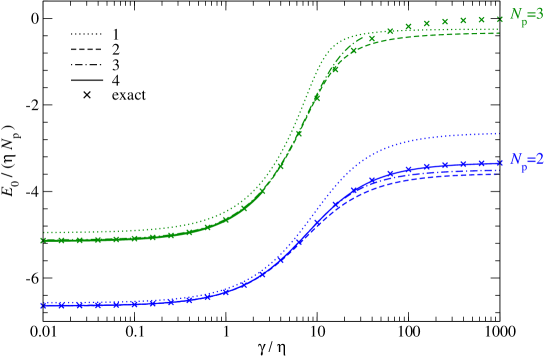
Figure 2: Ground-state energy per particle for the $2\times 3$ FNU hard-core boson Hubbard model with periodic boundary conditions versus the interaction strength $\gamma$ with $N_{\mathrm{p}}=2$ and $N_{\mathrm{p}}=3$ particles per spin. We compare the results from exact numerical diagonalization ($\times$) with those from present multinomial perturbative scheme by using cumulants up to order $k_{\mathrm{max}}=1,2,3,4$ (dotted, dashed, dot-dashed, solid lines, respectively).

The results obtained by using cumulants up to order $k_{\mathrm{max}}=1,2,3,4$ are shown in figure 2 as a function of the ratio $\gamma/\eta$ in the case of a lattice with $2\times 3$ sites and $N_{\mathrm{p}}=2,3$ particles per spin. In the same figure we also depict the values of $E_{0}$ determined by exact numerical diagonalization. The curves obtained for $k_{\mathrm{max}}=1$ coincide with the uncorrelated multinomial prediction and, as already noted, their behavior is only qualitatively correct. Already at $k_{\mathrm{max}}=2$, the quantitative agreement with the exact ground-state energy becomes impressive at least for values of $\gamma/\eta$ not too large. By further increasing $k_{\mathrm{max}}$, the quantitative agreement gradually improves in the whole range of $\gamma/\eta$ which, note the horizontal log scale, goes from the limit $\|\hat{V}\|\ll\|\hat{K}\|$ to the opposite one $\|\hat{V}\|\gg\|\hat{K}\|$. In the case with $N_{\mathrm{p}}=2$ particles per spin, the curve $E_{0}(\gamma)$ obtained with $k_{\mathrm{max}}=4$ is indistinguishable from the reported exact values. In the case with $N_{\mathrm{p}}=3$ particles per spin, the nonlinear equations (135-136) do not admit a solution for $k_{\mathrm{max}}=3,4$ when $\gamma/\eta$ is larger than a threshold value, namely $\gamma/\eta\simeq 31.6$ for $k_{\mathrm{max}}=3$ and $\gamma/\eta\simeq 2.5$ for $k_{\mathrm{max}}=4$. As discussed at the beginning of section 3, this means that the perturbative scheme is invalid at the order considered.

In figure 3 we show the results obtained with a system of larger size, namely a lattice $4\times 4$ with $N_{\mathrm{p}}=2,4,5,8$ particles. In this case, the number of configurations is so large, namely

$$M=\left(\frac{(L_{x}L_{y})!}{N_{\mathrm{p}}!(L_{x}L_{y}-N_{\mathrm{p}})!}\right)^{2},$$ (149)

that an exact numerical diagonalization of the Hamiltonian (142) is unfeasible. Therefore, we have compared the values of $E_{0}$ predicted by the present multinomial perturbative scheme with those obtained by a Monte Carlo simulation [7]. The conclusions that we reach from the analysis of figure 3 are similar to those we noticed after figure 2. However, for this larger system we see that the parity of the order $k_{\mathrm{max}}$ may influence the quality of the approximation, a fact which is not surprising. For instance, in the case with $N_{\mathrm{p}}=5$ it is evident that the curve $E_{0}(\gamma)$ obtained with $k_{\mathrm{max}}=3$ is not better than that obtained with $k_{\mathrm{max}}=2$. However, as evidenced in the enlargement shown in figure 4, the results obtained with $k_{\mathrm{max}}=4$ are more accurate than those with $k_{\mathrm{max}}=2$, at least in the $\gamma/\eta$ range where equations (135-136) admit the $k_{\mathrm{max}}=4$ solution.

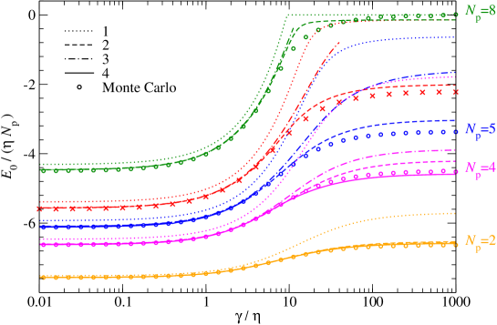
Figure 3: As in figure 2 in the case of a $4\times 4$ FNU hard-core boson Hubbard model with periodic boundary conditions and $N_{\mathrm{p}}=2,4,5,8$ particles per spin. The data indicated by $\circ$ have been obtained by Monte Carlo simulations [7] (the associated statistical errors increase with increasing $\gamma$ and are of the order of the symbol size at $\gamma\simeq 1000\eta$).

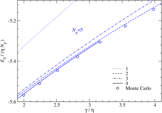
Figure 4: Enlargement of figure 3, case with $N_{\mathrm{p}}=5$. The perturbative scheme with $k_{\mathrm{max}}=4$ admits a solution only for $\gamma\lesssim 3.2\eta$ but in this range provides results more accurate than those obtained with $k_{\mathrm{max}}=1,2,3$.

6 Hubbard model with a magnetic field

In the examples considered in the previous section we have $\mathscr{L}=\{1\}$, i.e. the phase variables play no role. The situation is different in the case of fermions or for hard-core bosons in the presence of a magnetic field. In order to illustrate how to deal with the phase variables, in this section we will consider a Hubbard model in a one-dimensional lattice with periodic boundary conditions, namely a ring with $L$ sites, threaded by a line of magnetic flux $\phi$. In the case of spin 1/2 fermions, this is a well known model used to study electronic persistent currents, see [21] for a review. The model is free of sign problem in the case of an even number of fermions per spin. In order to concentrate on the effects due to the sole magnetic field, in the following we will therefore assume $N_{\mathrm{p}}$, the number of particles per spin, to be even. This is equivalent to consider a system of $N_{\mathrm{p}}+N_{\mathrm{p}}$ pseudo-spin 1/2 hard-core bosons.

The Hamiltonian of the system is

$$\hat{H}=-\eta\sum_{j=1}^{L}\sum_{\sigma=\uparrow\downarrow}\left(\mathrm{e}^{-\mathrm{i}\theta}\hat{c}_{j+1\sigma}^{\dagger}\hat{c}_{j\sigma}^{\phantom{\dagger}}+\mathrm{e}^{\mathrm{i}\theta}\hat{c}_{j\sigma}^{\dagger}\hat{c}_{j+1\sigma}^{\phantom{\dagger}}\right)+\gamma\sum_{j=1}^{L}\hat{c}_{j\uparrow}^{\dagger}\hat{c}_{j\uparrow}^{\phantom{\dagger}}\hat{c}_{j\downarrow}^{\dagger}\hat{c}_{j\downarrow}^{\phantom{\dagger}},$$ (150)

where site correspondence $j\pm L=j$ is assumed and $\mathrm{e}^{\pm\mathrm{i}\theta}$ are the Peierls phase factors with $\theta=2\pi\phi/(L\phi_{0})$, $\phi_{0}=h/(2e)$ being the magnetic flux quantum. The spectrum of the Hamiltonian (150) can be determined exactly in terms of the Bethe ansatz [22], however, when the Fock dimension $(L!/(N_{\mathrm{p}}!(L-N_{\mathrm{p}})!))^{2}$ is not too large, a numerical diagonalization represents a simpler alternative. The ground state energy $E_{0}$ as well as all the excited eigenenergies of $\hat{H}$ are periodic functions of the flux $\phi$ with period $\phi_{0}$. In the non-interacting case $\gamma=0$, the ground state energy $E_{0}^{(0)}$ has the simple expression

$$E_{0}^{(0)}(\phi)=-4\eta\frac{\sin(\pi N_{\mathrm{p}}/L)}{\sin(\pi/L)}\cos\left(\frac{2\pi}{L}\frac{\phi}{\phi_{0}}\right),\qquad\phi\in[-\phi_{0}/2,\phi_{0}/2].$$ (151)

The sets of the potential, hopping and phase variables which apply to the present model are found out at once. We have $\mathscr{V}=\{0,\gamma,2\gamma,\ldots,N_{\mathrm{p}}\gamma\}$, $\mathscr{T}=\{N_{\mathrm{p}}\eta,(N_{\mathrm{p}}+2)\eta,(N_{\mathrm{p}}+4)\eta,\dots,2N_{\mathrm{p}}\eta\}$ and $\mathscr{L}=\{\mathrm{e}^{\mathrm{i}\theta},\mathrm{e}^{-\mathrm{i}\theta}\}$. These data, together with the asymptotic rescaled cumulants $\bm{\Sigma}^{(k)}$ measured up to some order $k\leq k_{\mathrm{max}}$, are input into equations (135-136) to determine the ground-state energy $E_{0}$. Let us start considering the non-interacting case $\gamma=0$ at the lowest perturbative order $k_{\mathrm{max}}=1$. According to equation (138) and considering that $\mathscr{V}=\{0\}$ and $\Sigma_{\lambda=\mathrm{e}^{\mathrm{i}\theta}}^{(1)}=\Sigma_{\lambda=\mathrm{e}^{-\mathrm{i}\theta}}^{(1)}=1/2$ (for each forward movement of a particle in the ring there is another possible backward jump) we have

$$E_{0}^{(0)}=-\left(\sum_{T\in\mathscr{T}}\Sigma^{(1)}_{T}T\right)\cos\left(\frac{2\pi}{L}\frac{\phi}{\phi_{0}}\right).$$ (152)

Compared to the exact expression (151) this is a very promising result. However, equations (139), (140) and (141) show that, whereas $\nu_{V=0}^{\mathrm{sp}}=1$ and $0<\nu_{T}^{\mathrm{sp}}<1$ for $T\in\mathscr{T}$, as expected, the saddle-point frequencies associated with the phase variables $\lambda=\rme^{\pm\mathrm{i}\theta}$ are complex conjugated, namely

$$\nu_{\pm}^{\mathrm{sp}}=\frac{1}{2}\pm\frac{\mathrm{i}}{2}\tan\theta.$$ (153)

To simplify the notation, hereafter we use the subscripts $\pm$ instead of $\lambda=\mathrm{e}^{\pm\mathrm{i}\theta}$. The situation does not change for $\gamma\neq 0$ or at higher perturbative orders. From equation (136) we see that any $\nu_{\alpha}^{\mathrm{sp}}$ lies outside the real unit simplex. What is the meaning of these complex frequencies? Do they imply an unphysical complex solution for $E_{0}$?

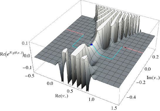
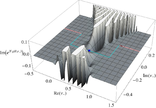
Figure 5: Real and imaginary parts of principal branch of $\exp(Ng(\theta,\nu_{-}))$ as a function of the complex variable $\nu_{-}$ for $N=35$ and $\theta=\pi/8$. A contour from $\nu_{-}=0$ to $\nu_{-}=1$ is shown which goes through the saddle point $\nu_{-}^{\mathrm{sp}}=(1-\mathrm{i}\tan\theta)/2$ in the direction of the steepest descent. The branch cuts $(-\infty,0]$ and $[1,\infty)$ along the real axis are also indicated.

To answer the above questions we re-examine the derivation of the fundamental equations (135-136) in the specific case of two phase variables. Let us start to consider the asymptotic evaluation of the integral (132) at the lowest pertubative order $k_{\mathrm{max}}=1$. The integral $I_{N}$ coincides with the generating function (59) provided we choose the source $\bm{J}=\bm{u}(E_{0})$, which in the present case reads

$$\bm{u}^{\mathrm{T}}(E_{0})=(\ldots-\log(-E_{0}+V)\ldots;\ldots\log T\ldots;\mathrm{i}\theta,-\mathrm{i}\theta).$$ (154)

For $k_{\mathrm{max}}=1$, the integral factorizes

$$I_{N}=I_{N,\mathscr{V}}~{}I_{N,\mathscr{T}}~{}I_{N,\mathscr{L}},$$ (155)

where for $\mathscr{A}=\mathscr{V},\mathscr{T},\mathscr{L}$, up to inessential constants, we have

$$I_{N,\mathscr{A}}=\int\prod_{\alpha\in\mathscr{A}}\mathrm{d}{\nu_{\alpha}}~{}\mathrm{e}^{N\sum_{\alpha\in\mathscr{A}}\nu_{\alpha}\left[\log\left(\frac{p^{(1)}_{\alpha}}{\nu_{\alpha}}\right)+u_{\alpha}\right]}\delta\left(\sum_{\alpha\in\mathscr{A}}\nu_{\alpha}-1\right),$$ (156)

For $\mathscr{A}=\mathscr{V},\mathscr{T}$ the functions to be integrated are real so that $I_{N,\mathscr{V}}$ and $I_{N,\mathscr{T}}$ can be evaluated asymptotically by the Laplace method as explained before. The corresponding saddle-points frequencies $\nu_{V}^{\mathrm{sp}}$, $V\in\mathscr{V}$, and $\nu_{T}^{\mathrm{sp}}$, $T\in\mathscr{T}$, are real and lie in the unit simplex. In the case of $I_{N,\mathscr{L}}$ we use the Dirac $\delta$ to eliminate the frequency $\nu_{+}=1-\nu_{-}$ and obtain

$$I_{N,\mathscr{L}}=\int_{0}^{1}\mathrm{d}{\nu_{-}}~{}\mathrm{e}^{Ng(\theta,\nu_{-})},$$ (157)

where

$$g(\theta,\nu_{-})=(1-\nu_{-})\log\left(\frac{1/2}{1-\nu_{-}}\right)+\nu_{-}\log\left(\frac{1/2}{\nu_{-}}\right)+\mathrm{i}\theta(1-2\nu_{-}).$$ (158)

Due to the factor $\mathrm{e}^{\mathrm{i}N\theta(1-2\nu_{-})}$, for $N$ large the integral (157) suffers from wild cancellations hard to estimate. However, $\exp(Ng(\theta,\nu_{-}))$ thought of as a function of the complex variable $\nu_{-}$ is analytic in the whole complex plane except the branch cuts $(-\infty,0]$ and $[1,\infty)$ along the real axis (we consider the principal branch). Thus we can evaluate (157) by deforming the integration contour in the complex plane. Any contour going from $\nu_{-}=0$ to $\nu_{-}=1$ and passing through the saddle point $\nu_{-}^{\mathrm{sp}}(\theta)=(1-\mathrm{i}\tan\theta)/2$, solution of the equation $\mathrm{d}{g(\theta,\nu_{-})}/\mathrm{d}{\nu_{-}}=0$, in the direction of the steepest descent provides the asymptotic logarithm equality

$$I_{N,\mathscr{L}}\simeq\mathrm{e}^{Ng(\theta,\nu_{-}^{\mathrm{sp}}(\theta))}=\mathrm{e}^{N\log(\cos\theta)}.$$ (159)

An example of the steepest descent contour is shown in figure 5. Note that, despite the complex nature of the saddle point $\nu_{-}^{\mathrm{sp}}$, the asymptotic result of the integration is real as required. It follows that the corresponding equation for the ground-state energy, obtained as $\lim_{N\to\infty}N^{-1}\log I_{N}(E_{0})=0$, with $E_{0}\leq V_{\mathrm{min}}$, explicitly gives

$$\sum_{V\in\mathscr{V}}\frac{\Sigma^{(1)}_{V}}{-E_{0}+V}=\frac{1}{\left(\sum_{T\in\mathscr{T}}\Sigma^{(1)}_{T}T\right)\cos\theta},\qquad E_{0}\leq V_{\mathrm{min}}.$$ (160)

This equation always admits one and only one real solution $E_{0}$.

At higher perturbative orders the situation is more complicated. The factorization (155) does not apply and the oscillating factor $\mathrm{e}^{\mathrm{i}N\theta(1-2\nu_{-})}$ affects, via the correlations induced by $\bm{p}(\bm{\nu})$, the evaluation of the integrals over all frequencies $\nu_{\alpha}$, $\alpha\in\mathscr{H}$. Once again, however, the asymptotics of $I_{N}$ is correctly estimated by the value of its integrand function at the complex saddle point $\bm{\nu}^{\mathrm{sp}}$ determined by equation (136). Despite $\bm{\nu}^{\mathrm{sp}}\in\mathbb{C}^{|\mathscr{H}|}$, we expect the asymptotic value of $I_{N}$ to be real and equation (135) to admit a real solution $E_{0}$. A mathematical justification for the saddle-point method in $\mathbb{C}^{|\mathscr{H}|}$ is given by theorem 2.8 of [23].

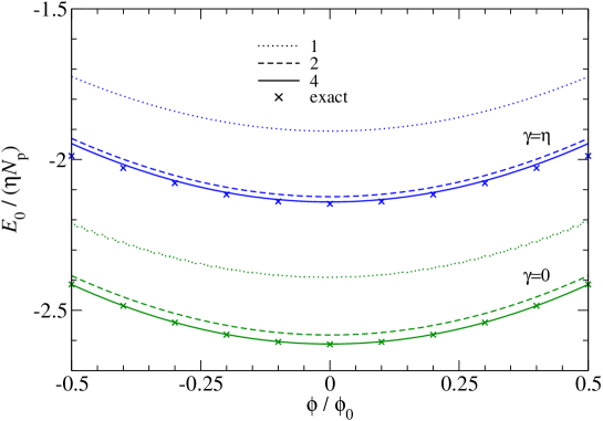
Figure 6: Ground-state energy per particle for the FNU pseudo-spin 1/2 hard-core boson Hubbard model in a ring threaded by a magnetic flux $\phi$. The ring has $L=8$ sites and the number of particles per spin is $N_{\mathrm{p}}=4$. Exact values of $E_{0}$ ($\times$) are compared with the results from present multinomial perturbative scheme by using cumulants up to order $k_{\mathrm{max}}=1,2,4$ (dotted, dashed, solid lines, respectively) for two different values of the interaction strength $\gamma$.

We have checked the scenario depicted above by numerical simulations on the model described by the Hamiltonian (150). In figure 6 we show the behavior of $E_{0}(\phi)$ determined at perturbative orders $k_{\mathrm{max}}=1,2,4$ in comparison with the exact values of the ground-state energy obtained by numerical diagonalization of $\hat{H}$. In all cases the solution of the system of equations (135-136) in terms of complex unknowns $(E_{0},\bm{\nu}^{\mathrm{sp}})$ provides a ground-state energy which is real within the statistical errors associated with the input cumulants. The agreement with the exact values of $E_{0}(\phi)$ increases on increasing the perturbative order in the whole range of the magnetic flux. At $\gamma=0$ the solution for $k_{\mathrm{max}}=4$ is practically exact. When hopping and interaction have equal strengths, i.e. for $\gamma=\eta$, the $k_{\mathrm{max}}=4$ solution is in excellent agreement with $E_{0}(\phi)$ at small fluxes. At the flux edges $\phi=\pm\phi_{0}/2$ a residual error of about $2\%$ is observed. Note that for systems of larger size we have smaller maximum phases $\theta=\pi/L$ and therefore we expect a better performance of our approach already at small perturbative orders. Of course at large sizes the measurement of the input cumulant is statistically heavier.

7 Conclusions

In the framework of the probabilistic approach previously developed by us to study the ground-state properties of many-body quantum systems, we have introduced a multinomial perturbative scheme which has the following characteristics. At any perturbative order, the probability distribution of the potential, hopping and phase multiplicities, whose knowledge would allow for an exact solution of the problem, is approximated by a multinomial-like distribution with infinitely many statistical moments. By increasing the perturbative order, an increasing number of cumulants of the distribution is made to coincide with the corresponding exact cumulants of the system.

We have tested the proposed perturbative scheme in the case of Hubbard models with pseudo-spin 1/2 hard-core bosons in two-dimensional lattices and in a ring threaded by a magnetic flux.

For the two-dimensional lattices, we find, already at second perturbative order, a ground-state energy in good quantitative agreement with the exact one for any value of the ratio $\gamma/\eta$, $\gamma$ and $\eta$ being the strengths of the interaction and hopping terms of the Hamiltonian of the system. The agreement improves at higher perturbative orders. At orders $\geq 3$, however, the scheme may not always be consistent, i.e. in some systems a solution for the ground-state energy is found only for values of $\gamma/\eta$ smaller than a threshold. As a matter of fact, we observe that in all our test cases at, or near, the $\nicefrac{{1}}{{4}}$ particle filling, which is a case of remarkable physical interest, the solution of the perturbative method turns out to exist for all values of the interaction parameter up to the largest explored perturbative order, $k_{\mathrm{max}}=4$, where it provides stunning results.

The ring-shaped one-dimensional lattice with an orthogonal magnetic field is a well known model to study electronic persistent currents and, remarkably, presents a phase problem. For this model we discuss in detail how our approach handles the phase problem and allow to find the correct behavior of the ground-state energy as a function of the threading flux $\phi$. As in the previous phase-problem–free cases, the quantitative agreement of $E_{0}(\phi)$ with the corresponding exact values increases on increasing the perturbative order both for non-interacting or interacting systems.

The limits, merits and scaling properties of our approach can be summarized as follows.

The main uncertainty is that we do not know a priori if our perturbative scheme is meaningful at any order. For the systems considered here, the second perturbative order always provides a fairly accurate ground-state energy. Sometimes, at third and fourth order the nonlinear system of equations which must be solved to find $E_{0}$ does not admit a solution. An increased statistical accuracy of the input data used to define the coefficients of these equations and/or more accurate numerical methods to solve the system of equations (135-136) could relieve this problem.

In our approach, the perturbative probability distribution at order $k$ is built up from the knowledge of the first $k$ connected statistical moments of the potential, hopping and phase multiplicities of the system. These cumulants, more precisely the associated asymptotic rescaled cumulants, are measured by Monte Carlo simulations as explained in [11]. We use initial configurations randomly distributed according to the invariant measure of the Markov chain which provides their evolution. Thus, in a sense, ours is a perfect simulation [24]. Moreover, the mentioned Markov chain has a finite correlation length which grows slowly, at least for the cases studied, with the size of the system. This implies that sampling cumulants of relatively high order is statistically reliable also for large size systems. Our statistical accuracy, however, could be increased by faster unbiased estimators based on the umbral calculus [25]. In the present paper, the highest cumulant order considered is 4 merely because the perturbative coefficients $\bm{p}^{(k)}$ have been explicitly calculated only up to $k=4$.

It is difficult to precisely assess the scaling of the computational costs of our method with the size $S$ of the system considered. Unquestionably, the cardinality of the set $\mathscr{H}$ grows only linearly with $S$ so that the evaluation of the cumulants of order $k$ can be safely bounded by $S^{k}$. However, from the limited data at our disposal it is rash to figure out the behavior of $k_{\mathrm{max}}(\varepsilon,S)$, the maximum order $k$ needed to calculate $E_{0}$ at size $S$ with error $\epsilon$.

The cumulants input into equations (135-136) are independent of the parameters $\gamma$ and $\eta$, namely the strengths of the interaction and hopping terms of the Hamiltonian of the system. Once the probability distribution is determined at the chosen approximation, the ground-state energy $E_{0}$ can be found by solving numerically a small system of nonlinear equations. The latter job has a computational cost negligible with respect to the determination of the cumulants, which, in turn, has a cost roughly equivalent to a direct Monte Carlo evaluation of $E_{0}$. Thus, the advantage of our approach in comparison to a direct Monte Carlo simulation is remarkable. Different Monte Carlo runs are needed to evaluate $E_{0}$ for different values of $\eta$ and/or $\gamma$, whereas in our approach we have to solve each time a small system of nonlinear equations and, una tantum, calculate the cumulants.

Another advantage of our approach is that no extra efforts are required to evaluate generic ground-state correlation functions. The key point is, again, the analytical dependence of our equations (135-136), and, therefore, of its solution $E_{0}$, on $\gamma$ and $\eta$ as well as on any other parameter entering the Hamiltonian of the system. In fact, the quantum expectation of an observable $\hat{O}$ in the ground state of $\hat{H}$ is reconduced, via the Hellman-Feynman theorem, to the ability to take the derivative with respect to the parameter $\xi$ of the ground-state energy of the ancillary Hamiltonian $\hat{H}+\xi\hat{O}$.

The present perturbative probabilistic approach is particularly promising for systems affected by the so called sign problem, for which unbiased Monte Carlo simulations of $E_{0}$ are impractical. In fact, the statistical evaluation of the cumulants of the potential, hopping and phase multiplicities is unaffected by sign/phase problems. Oscillations and cancellations remain confined in the expression of the perturbative probability distribution and can be tackled by complex analysis techniques. Here, we have provided an example of this strategy in a somewhat softer phase problem. We plan to discuss the case of fermions in a future paper.

Appendix A Solution of nonsymmetric algebraic Riccati equations

In section 3.4 we have seen that the parameters $\bm{p}^{(2)}$, more precisely the associated reduced matrix $\hat{\bm{p}}^{(2)}$, are determined by the NARE (107). In general, the NAREs are defined as the quadratic matrix equations of the kind

$$\bm{X}\bm{C}\bm{X}-\bm{A}\bm{X}-\bm{X}\bm{D}+\bm{B}=\bm{0},$$ (161)

where we assume that the unknown $\bm{X}$, as well as the coefficients $\bm{A}$, $\bm{B}$, $\bm{C}$ and $\bm{D}$ are quadratic matrices of finite size. In this section we illustrate two numerical methods developed to solve equation (161). The first one is an iterative method based on a fixed-point technique [26], whereas the second one is a direct method based on the Schür decomposition [17].

Equations (161) play an important role in the study of the stochastic fluid models and have been extensively studied. In general, a NARE admits more than one solution. In most stochastic fluid models, the coefficients $\bm{A}$, $\bm{B}$, $\bm{C}$ and $\bm{D}$ form a super matrix

$$\bm{H}=\left(\begin{array}[]{cc}\bm{D}&-\bm{C}\\ -\bm{B}&\bm{A}\end{array}\right).$$ (164)

with the property to be a so called $M$-matrix [17]. It can be proved that in this case the Schür method provides the minimal non negative solution of the NARE, which is, there, the solution of physical interest.

In our context, $\bm{H}$ is not a $M$-matrix and it is not clear which solution of the NARE (107) has to be considered. We propose to consider the unique solution given by the Schür method. This solution coincides with that obtained by the iterative method in which $\bm{X}$ is chosen at the zeroth iteration as the solution of (161) with $\bm{C}=\bm{0}$. Since in our case $\bm{X}$ represents the matrix of the perturbative parameters $\hat{\bm{p}}^{(2)}$, which we expect to be small, the above proposed solution seems the most natural one.

A.1 Iterative method

In [26] a class of fixed-point methods is considered to solve equation (161). These fixed-point iterations are based on a suitable splitting of the matrices $\bm{A}$ and $\bm{D}$, that is $\bm{A}=\bm{A}_{1}-\bm{A}_{2}$ and $\bm{D}=\bm{D}_{1}-\bm{D}_{2}$, and have the form

$$\bm{A}_{1}\bm{X}_{k+1}+\bm{X}_{k+1}\bm{D}_{1}=\bm{X}_{k}\bm{C}\bm{X}_{k}+\bm{A}_{2}\bm{X}_{k}+\bm{X}_{k}\bm{D}_{2}+\bm{B},$$ (165)

with $k=0,1,2,\dots$ and $\bm{X}_{0}=\bm{0}$. In particular, for $\bm{A}_{1}=\bm{A}$ and $\bm{D}_{1}=\bm{D}$ we have

$$\bm{A}\bm{X}_{k+1}+\bm{X}_{k+1}\bm{D}=\bm{X}_{k}\bm{C}\bm{X}_{k}+\bm{B},\qquad\bm{X}_{0}=\bm{0}.$$ (166)

Note that finding $\bm{X}_{k+1}$ in terms of $\bm{X}_{k}$ at $k$th iteration implies to solve a Sylvester equation. This can be accomplished by vectorization, namely

$$\mathrm{vec}\left(\bm{A}\bm{X}_{k+1}\right)+\mathrm{vec}\left(\bm{X}_{k+1}\bm{D}\right)=\mathrm{vec}\left(\bm{X}_{k}\bm{C}\bm{X}_{k}+\bm{B}\right).$$ (167)

Using the properties of the $\mathrm{vec}$ operator, in particular

$$\mathrm{vec}\left(\bm{A}\bm{X}_{k+1}\right)=\left(\bm{I}\otimes\bm{A}\right)\mathrm{vec}\left(\bm{X}_{k+1}\right),$$ (168)

$$\mathrm{vec}\left(\bm{X}_{k+1}\bm{D}\right)=\left(\bm{D}^{T}\otimes\bm{I}\right)\mathrm{vec}\left(\bm{X}_{k+1}\right),$$ (169)

where $\otimes$ indicates the Kronecker product and ^T the transpose, equation (167) is rewritten as

$$\left[\left(\bm{I}\otimes\bm{A}\right)+\left(\bm{D}^{T}\otimes\bm{I}\right)\right]\mathrm{vec}\left(\bm{X}_{k+1}\right)=\mathrm{vec}\left(\bm{X}_{k}\bm{C}\bm{X}_{k}+\bm{B}\right).$$ (170)

This is a linear matrix equation which can be solved by standard methods, e.g. LU-factorization [18].

The convergence of the full class of iterative schemes (165) to a solution $\bm{X}$ of (161) is ensured by a theorem [26]. In this class, the iterative scheme (166) is the most expensive from a computational point of view, but, on the other hand, it has the highest (linear) convergence speed.

A.2 Schür method

In the following we discuss a different approach to solve equation (161), based on the ordered Schür decomposition. This approach was conceived by Laub [16] for a symmetric algebraic Riccati equation and extended by Guo [27] to the study of NAREs.

Let us rewrite the matrix $\bm{H}$ associated with the coefficients of (161) as

$$\bm{H}=\left(\begin{array}[]{cc}\bm{D}&-\bm{C}\\ -\bm{B}&\bm{A}\end{array}\right)=\left(\begin{array}[]{cc}\bm{H}_{11}&\bm{H}_{12}\\ \bm{H}_{21}&\bm{H}_{22}\end{array}\right).$$ (175)

Note that $\bm{H}$ is real in our case. We look for an orthogonal transformation

$$\bm{U}=\left(\begin{array}[]{cc}\bm{U}_{11}&\bm{U}_{12}\\ \bm{U}_{21}&\bm{U}_{22}\end{array}\right),$$ (178)

which leaves $\bm{H}$ in a semi-ordered real Schür form,

$$\bm{U}^{T}\bm{H}\bm{U}=\bm{S}=\left(\begin{array}[]{cc}\bm{S}_{11}&\bm{S}_{12}\\ \bm{0}&\bm{S}_{22}\end{array}\right),$$ (181)

in which $\bm{S}_{11}$ and $\bm{S}_{22}$ contain only blocks, denoted $\bm{s}_{ij}$, $i,j=1,2,\dots$, of size 1 or 2. The eigenvalues of the $2\times 2$ diagonal blocks $\bm{s}_{ii}$ provide the complex conjugated eigenvalues of $\bm{H}$ whereas the $1\times 1$ blocks are the real eigenvalues of $\bm{H}$. The diagonal blocks are semi-ordered in the sense that if $\bm{s}_{ii}$, $\bm{s}_{jj}$ and $\bm{s}_{kk}$ have eigenvalues with positive, null and negative real parts, respectively, then $i<j<k$. It is possible to show that the matrix $\bm{U}_{11}$ is invertible and that

$$\bm{X}=\bm{U}_{21}\bm{U}_{11}^{-1}$$ (182)

solves (161). Note that the semi-ordered decomposition (181) is unique and so is the solution (182). We used the subroutines of LAPACK library [28] to numerically implement the Schür method.

Appendix B Equations for the perturbative parameters: fourth order

The perturbative parameters $\bm{p}^{(4)}$ are determined by the system of equations

$$\langle\!\langle\nu_{\alpha_{1}}\nu_{\alpha_{2}}\nu_{\alpha_{3}}\nu_{\alpha_{4}}\rangle\!\rangle(\bm{p}^{(1)},\bm{p}^{(2)},\bm{p}^{(3)},\bm{p}^{(4)})=\Sigma_{\alpha_{1}\alpha_{2}\alpha_{3},\alpha_{4}}^{(4)},$$ (183)

with $\alpha_{1},\alpha_{2},\alpha_{3},\alpha_{4}\in\mathscr{H}$. By using (76) and taking the derivative of (85) with respect to $J_{\alpha_{4}}$, the above system can be cast in the form

$$\sum_{\alpha\in\mathscr{H}}\sum_{\beta\in\mathscr{H}}\sum_{\gamma\in\mathscr{H}}\sum_{\delta\in\mathscr{H}}\left(\Lambda^{(2,0)}_{{\alpha}_{1}\alpha}\Sigma^{(2)}_{\beta{\alpha}_{2}}\Sigma^{(2)}_{\gamma{\alpha}_{3}}\Sigma^{(2)}_{\delta{\alpha}_{4}}+\Sigma^{(2,0)}_{{\alpha}_{1}\alpha}\Lambda^{(2)}_{\beta{\alpha}_{2}}\Sigma^{(2)}_{\gamma{\alpha}_{3}}\Sigma^{(2)}_{\delta{\alpha}_{4}}\right.$$

$$+\left.\Sigma^{(2,0)}_{{\alpha}_{1}\alpha}\Sigma^{(2)}_{\beta{\alpha}_{2}}\Lambda^{(2)}_{\gamma{\alpha}_{3}}\Sigma^{(2)}_{\delta{\alpha}_{4}}+\Sigma^{(2,0)}_{{\alpha}_{1}\alpha}\Sigma^{(2)}_{\beta{\alpha}_{2}}\Sigma^{(2)}_{\gamma{\alpha}_{3}}\Lambda^{(2)}_{\delta{\alpha}_{4}}\right)p^{(4)}_{\alpha\beta\gamma\delta}=\Delta_{{\alpha}_{1}{\alpha}_{2}{\alpha}_{3}{\alpha}_{4}},$$ (184)

where $\mathbf{\Sigma}^{(2)}$ is the asymptotic rescaled cumulant of order 2 and the matrices $\mathbf{\Sigma}^{(2,0)}$, $\mathbf{\Lambda}^{(2)}$ and $\mathbf{\Lambda}^{(2,0)}$ are defined by (95), (112) and (113), respectively. The tensor $\bm{\Delta}$ has components $\alpha_{1},\alpha_{2},\alpha_{3},\alpha_{4}\in\mathscr{H}$ given by

$$\Delta_{\alpha_{1}\alpha_{2}\alpha_{3}\alpha_{4}}=\Sigma^{(4)}_{\alpha_{1}\alpha_{2}\alpha_{3}\alpha_{4}}-\Sigma^{(4,0)}_{\alpha_{1}\alpha_{2}\alpha_{3}\alpha_{4}}$$

$$-\sum_{\alpha\in\mathscr{H}}\sum_{\beta\in\mathscr{H}}\left(\Sigma^{(2,0)}_{\alpha_{1}\alpha}M^{(2)}_{\alpha\beta}\Sigma^{(4)}_{\beta\alpha_{2}\alpha_{3}\alpha_{4}}+\Sigma^{(4,0)}_{\alpha_{1}\alpha\alpha_{3}\alpha_{4}}M^{(2)}_{\alpha\beta}\Sigma^{(2)}_{\beta\alpha_{2}}\right)$$

$$-\sum_{\alpha\in\mathscr{H}}\sum_{\beta\in\mathscr{H}}\Sigma^{(3,0)}_{\alpha_{1}\alpha\alpha_{3}}\left(M^{(3)}_{\alpha\beta\alpha_{4}}\Sigma^{(2)}_{\beta\alpha_{2}}+M^{(2)}_{\alpha\beta}\Sigma^{(3)}_{\beta\alpha_{2}\alpha_{4}}\right)$$

$$-\sum_{\alpha\in\mathscr{H}}\sum_{\beta\in\mathscr{H}}\Sigma^{(3,0)}_{\alpha_{1}\alpha\alpha_{4}}\left(M^{(3)}_{\alpha\beta\alpha_{3}}\Sigma^{(2)}_{\beta\alpha_{2}}+M^{(2)}_{\alpha\beta}\Sigma^{(3)}_{\beta\alpha_{2}\alpha_{3}}\right)$$

$$-\sum_{\alpha\in\mathscr{H}}\sum_{\beta\in\mathscr{H}}\Sigma^{(2,0)}_{\alpha_{1}\alpha}\left(M^{(3)}_{\alpha\beta\alpha_{3}}\Sigma^{(3)}_{\beta\alpha_{2}\alpha_{4}}+M^{(3)}_{\alpha\beta\alpha_{4}}\Sigma^{(3)}_{\beta\alpha_{2}\alpha_{3}}\right)$$

$$-\sum_{\alpha\in\mathscr{H}}\sum_{\beta\in\mathscr{H}}\sum_{\gamma\in\mathscr{H}}\Sigma^{(2,0)}_{\alpha_{1}\alpha}F^{(3)}_{\alpha\beta\gamma}\Sigma^{(2)}_{\beta\alpha_{2}}\Sigma^{(3)}_{\gamma\alpha_{3}\alpha_{4}}$$

$$+\sum_{\alpha\in\mathscr{H}}\sum_{\beta\in\mathscr{H}}\sum_{\gamma\in\mathscr{H}}\sum_{\delta\in\mathscr{H}}\Sigma^{(2,0)}_{\alpha_{1}\alpha}F^{(4)}_{\alpha\beta\gamma\delta}\Sigma^{(2)}_{\beta\alpha_{2}}\Sigma^{(2)}_{\gamma\alpha_{3}}\Sigma^{(2)}_{\delta\alpha_{4}},$$ (185)

where

$$\Sigma^{(4,0)}_{\alpha\beta\gamma\delta}=\Sigma^{(3)}_{\beta\gamma\delta}\delta_{\alpha\beta}-\left(\Sigma^{(3)}_{\alpha\gamma\delta}\Sigma^{(1)}_{\beta}+\Sigma^{(3)}_{\beta\gamma\delta}\Sigma^{(1)}_{\alpha}+\Sigma^{(2)}_{\alpha\delta}\Sigma^{(2)}_{\beta\gamma}+\Sigma^{(2)}_{\alpha\gamma}\Sigma^{(2)}_{\beta\delta}\right)\chi_{\alpha\beta},$$ (186)

$$M^{(2)}_{\alpha\beta}=\left.M_{\alpha\beta}\left(\bm{\nu}^{\mathrm{sp}}\right)\right|_{\bm{J}=\bm{0}}=\frac{p^{(2)}_{\alpha\beta}}{\Sigma^{(1)}_{\alpha}}+\frac{p^{(2)}_{\alpha\beta}}{\Sigma^{(1)}_{\beta}}-\sum_{\gamma\in\mathscr{H}}\frac{p^{(2)}_{\alpha\gamma}p^{(2)}_{\gamma\beta}}{\Sigma^{(1)}_{\gamma}},$$ (187)

$$M^{(3)}_{\alpha\beta\gamma}=\left.\frac{\partial M_{\alpha\beta}(\bm{\nu}^{\mathrm{sp}})}{\partial J_{\gamma}}\right|_{\bm{J}=\bm{0}}=\sum_{\delta\in\mathscr{H}}F^{(3)}_{\alpha\beta\delta}\Sigma^{(2)}_{\delta\gamma},$$ (188)

$$F^{(3)}_{\alpha\beta\gamma}=\frac{p^{(3)}_{\alpha\beta\gamma}}{\Sigma^{(1)}_{\alpha}}+\frac{p^{(3)}_{\alpha\beta\gamma}}{\Sigma^{(1)}_{\beta}}+\frac{p^{(3)}_{\alpha\beta\gamma}}{\Sigma^{(1)}_{\gamma}}-\frac{p^{(2)}_{\alpha\beta}p^{(2)}_{\alpha\gamma}}{{\Sigma^{(1)}_{\alpha}}^{2}}-\frac{p^{(2)}_{\alpha\beta}p^{(2)}_{\beta\gamma}}{{\Sigma^{(1)}_{\beta}}^{2}}-\frac{p^{(2)}_{\alpha\gamma}p^{(2)}_{\gamma\beta}}{{\Sigma^{(1)}_{\gamma}}^{2}}$$

$$-\sum_{\delta\in\mathscr{H}}\left(\frac{p^{(3)}_{\alpha\beta\delta}p^{(2)}_{\delta\gamma}}{\Sigma^{(1)}_{\delta}}+\frac{p^{(3)}_{\alpha\delta\gamma}p^{(2)}_{\delta\beta}}{\Sigma^{(1)}_{\delta}}+\frac{p^{(3)}_{\delta\beta\gamma}p^{(2)}_{\alpha\delta}}{\Sigma^{(1)}_{\delta}}-2\frac{p^{(2)}_{\alpha\delta}p^{(2)}_{\delta\beta}p^{(2)}_{\delta\gamma}}{{\Sigma^{(1)}_{\delta}}^{2}}\right),$$ (189)

$$F^{(4)}_{\alpha\beta\gamma\delta}=\frac{p_{\alpha\beta\gamma}^{(3)}p_{\alpha\delta}^{(2)}+p_{\alpha\beta\delta}^{(3)}p_{\alpha\gamma}^{(2)}+p_{\alpha\gamma\delta}^{(3)}p_{\alpha\beta}^{(2)}}{{\Sigma_{\alpha}^{(1)}}^{2}}+\frac{p_{\alpha\beta\gamma}^{(3)}p_{\beta\delta}^{(2)}+p_{\alpha\beta\delta}^{(3)}p_{\beta\gamma}^{(2)}+p_{\beta\gamma\delta}^{(3)}p_{\alpha\beta}^{(2)}}{{\Sigma_{\beta}^{(1)}}^{2}}$$

$$+\frac{p_{\alpha\beta\gamma}^{(3)}p_{\gamma\delta}^{(2)}+p_{\alpha\gamma\delta}^{(3)}p_{\gamma\beta}^{(2)}+p_{\beta\gamma\delta}^{(3)}p_{\alpha\gamma}^{(2)}}{{\Sigma_{\gamma}^{(1)}}^{2}}+\frac{p_{\alpha\beta\delta}^{(3)}p_{\delta\gamma}^{(2)}+p_{\alpha\delta\gamma}^{(3)}p_{\delta\beta}^{(2)}+p_{\delta\beta\gamma}^{(3)}p_{\alpha\delta}^{(2)}}{{\Sigma_{\delta}^{(1)}}^{2}}$$

$$-2\left(\frac{p_{\alpha\beta}^{(2)}p_{\alpha\gamma}^{(2)}p_{\alpha\delta}^{(2)}}{{\Sigma_{\alpha}^{(1)}}^{3}}+\frac{p_{\alpha\beta}^{(2)}p_{\beta\gamma}^{(2)}p_{\beta\delta}^{(2)}}{{\Sigma_{\beta}^{(1)}}^{3}}+\frac{p_{\alpha\gamma}^{(2)}p_{\gamma\beta}^{(2)}p_{\gamma\delta}^{(2)}}{{\Sigma_{\gamma}^{(1)}}^{3}}+\frac{p_{\alpha\delta}^{(2)}p_{\delta\beta}^{(2)}p_{\delta\gamma}^{(2)}}{{\Sigma_{\delta}^{(1)}}^{3}}\right)$$

$$+\sum_{\varepsilon\in\mathscr{H}}\left[\frac{p_{\alpha\beta\varepsilon}^{(3)}p_{\varepsilon\gamma\delta}^{(3)}+p_{\alpha\varepsilon\gamma}^{(3)}p_{\varepsilon\beta\delta}^{(3)}+p_{\varepsilon\beta\gamma}^{(3)}p_{\varepsilon\alpha\delta}^{(3)}}{\Sigma_{\varepsilon}^{(1)}}\right.$$

$$-2\left(\frac{p_{\alpha\beta\varepsilon}^{(3)}p_{\varepsilon\gamma}^{(2)}p_{\varepsilon\delta}^{(2)}+p_{\alpha\varepsilon\gamma}^{(3)}p_{\varepsilon\beta}^{(2)}p_{\varepsilon\delta}^{(2)}+p_{\varepsilon\beta\gamma}^{(3)}p_{\alpha\varepsilon}^{(2)}p_{\varepsilon\delta}^{(2)}}{{\Sigma_{\varepsilon}^{(1)}}^{2}}\right.$$

$$+\left.\frac{p_{\alpha\varepsilon\delta}^{(3)}p_{\varepsilon\beta}^{(2)}p_{\varepsilon\gamma}^{(2)}+p_{\varepsilon\beta\delta}^{(3)}p_{\varepsilon\alpha}^{(2)}p_{\varepsilon\gamma}^{(2)}+p_{\varepsilon\gamma\delta}^{(3)}p_{\varepsilon\alpha}^{(2)}p_{\varepsilon\beta}^{(2)}}{{\Sigma_{\varepsilon}^{(1)}}^{2}}\right)+\left.6\frac{p_{\varepsilon\alpha}^{(2)}p_{\varepsilon\beta}^{(2)}p_{\varepsilon\gamma}^{(2)}p_{\varepsilon\delta}^{(2)}}{{\Sigma^{(1)}_{\varepsilon}}^{3}}\right].$$ (190)

To find $\bm{p}^{(4)}$, we first determine the reduced tensor $\hat{\bm{p}}^{(4)}$ which is the solution of the linear system

$$\sum_{\alpha\in\hat{\mathscr{H}}}\sum_{\beta\in\hat{\mathscr{H}}}\sum_{\gamma\in\hat{\mathscr{H}}}\sum_{\delta\in\hat{\mathscr{H}}}\left(\widetilde{\Lambda}_{{\alpha}_{1}\alpha}^{(2,0)}\widetilde{\Sigma}_{\beta{\alpha}_{2}}^{(2)}\widetilde{\Sigma}_{\gamma{\alpha}_{3}}^{(2)}\widetilde{\Sigma}_{\delta{\alpha}_{4}}^{(2)}+\widetilde{\Sigma}_{{\alpha}_{1}\alpha}^{(2,0)}\widetilde{\Lambda}_{\beta{\alpha}_{2}}^{(2)}\widetilde{\Sigma}_{\gamma{\alpha}_{3}}^{(2)}\widetilde{\Sigma}_{\delta{\alpha}_{4}}^{(2)}\right.$$

$$+\left.\widetilde{\Sigma}_{{\alpha}_{1}\alpha}^{(2,0)}\widetilde{\Sigma}_{\beta{\alpha}_{2}}^{(2)}\widetilde{\Lambda}_{\gamma{\alpha}_{3}}^{(2)}\widetilde{\Sigma}_{\delta{\alpha}_{4}}^{(2)}+\widetilde{\Sigma}_{{\alpha}_{1}\alpha}^{(2,0)}\widetilde{\Sigma}_{\beta{\alpha}_{2}}^{(2)}\widetilde{\Sigma}_{\gamma{\alpha}_{3}}^{(2)}\widetilde{\Lambda}_{\delta{\alpha}_{4}}^{(2)}\right)\hat{p}_{\alpha\beta\gamma\delta}^{(4)}=\Delta_{{\alpha}_{1}{\alpha}_{2}{\alpha}_{3}{\alpha}_{4}},$$ (191)

with $\alpha_{1},\alpha_{2},\alpha_{3},\alpha_{4}\in\hat{\mathscr{H}}$. The matrices $\widetilde{\bm{\Sigma}}^{(2)}$, $\widetilde{\bm{\Sigma}}^{(2,0)}$, $\widetilde{\bm{\Lambda}}^{(2)}$ and $\widetilde{\bm{\Lambda}}^{(2,0)}$ are defined by (102), (104), (116) and (117), respectively. The complete fourth-order perturbative parameter $\bm{p}^{(4)}$ is then recovered using the sum rules (93) for $k=4$.

References

References

[1] De Angelis G F, Jona-Lasinio G and Sirugue M, 1983
J. Phys. A: Math. Gen.16 2433
[2] De Angelis G F, Jona-Lasinio G and Sidoravicius V, 1998
J. Phys. A: Math. Gen.31 289
[3] Beccaria M, Presilla C, De Angelis G F and
Jona-Lasinio G, 1999
Europhys. Lett.48 243
[4] Beccaria M, Presilla C, De Angelis G F and
Jona-Lasinio G, 2000
Nucl. Phys. B83/84 911-913
[5] Beccaria M, Presilla C, De Angelis G F and
Jona-Lasinio G, 2001
Int. J. Mod. Phys. B15 1740
[7] Ostilli M and Presilla C, 2004
J. Phys. A: Math. Gen.38 405
[8] Ceperley D M, Kalos M H, 1986
Monte Carlo Methods in Statistical Physics
ed H Binder (Heidelberg: Springer) pp 145–194
[9] Ostilli M and Presilla C, 2004
New J. Phys.6 107
[10] Presilla C and Ostilli M, 2006
Int. J. Mod. Phys. B 20 2770
[11] Ostilli M and Presilla C, 2005
J. Stat. Mech. P04007
[12] Ostilli M and Presilla C, 2006
J. Stat. Mech. P11012
[13] Kingman J F C, 1993
Poisson Processes (Oxford: Clarendon)
[14] Bremaud P, 1999
Markov Chains, Gibbs Field, Monte Carlo Simulation, and Queues
(New York: Springer)
[15] Shiryayev A N, 1984
Probability (New York: Springer)
[16] Laub A J, 1979
IEEE Trans. Automat. Control24(6) 913
[17] Bini D A, Iannazzo B, Meini B, Poloni F, 2010
Matrix methods: theory, algorithms and applications
ed V Olshevsky and E Tyrtyshnikov (Singapore: World Scientic)
pp 176–209
[18] Press W H, Teukolsky S A, Vetterling W T, Flannery B P, 1992
Numerical Recipes, The art of Scientific Computing
2nd edn (Cambridge: Cambridge University Press)
[19] Hubbard J, 1963
Proc. Roy. Soc. A276 238
[20] Giuliani A, Mastropietro V, 2010
Comm. Math. Phys.293 301
[21] Viefers S, Koskinen P, Singha Deo P, Manninen M, 2004
Physica E21 1
[22] Lieb E H, Wu F Y, 1968
Phys. Rev. Lett.20 1445