A new EFT approach to NN scattering problem

Abstract

We present the new, modified Weinberg approach to the NN scattering problem in effective field theory. Issues of renormalization are briefly discussed and the results of LO calculations are presented.

1 Introduction

The few-nucleon sector of baryon chiral perturbation theory was first considered in Ref. Weinberg:rz (For a recent review see e.g. Epelbaum:2008ga ). Within Weinberg’s approach, the nucleon-nucleon (NN) potential is defined as a sum of all two-nucleon-irreducible time ordered diagrams of the non-relativistic effective field theory (EFT). It is calculated as a systematic expansion in small parameters. A finite number of diagrams contribute in the effective potential up to any finite order. The scattering amplitude is obtained by solving the Lippmann-Schwinger (LS) equation

$${T(\vec{p}\,^{\prime},\vec{p},k)=V(\vec{p}\,^{\prime},\vec{p})+\hbar\,m\int\frac{d^{3}\vec{q}}{(2\,\pi)^{3}}\,V(\vec{p}\,^{\prime},\vec{q})\,\frac{1}{\vec{p}^{2}-\vec{q}^{2}+i\,\epsilon}\,T(\vec{q},\vec{p},k),}$$ (1)

where ${\hbar}$ is included to keep the trace of the loop integration. The leading order NN potential is given by

$$V_{0}=C_{S}+C_{T}\,\vec{\sigma}_{1}\cdot\vec{\sigma}_{2}-\frac{g_{A}^{2}}{4\,F^{2}}\ \vec{\tau}_{1}\cdot\vec{\tau}_{2}\ \frac{\vec{\sigma}_{1}\cdot\vec{q}\,\vec{\sigma}_{2}\cdot\vec{q}}{q^{2}+M_{\pi}^{2}},$$ (2)

with standard notations.

2 Renormalization

In EFT, all divergences appearing in loop diagrams are absorbed in parameters of the effective Lagrangian. While non-perturbative expressions may contain pieces which do not contribute in perturbative series, perturbative expansion of properly renormalized EFT amplitudes in the region of applicability of perturbation theory must reproduce the properly renormalized perturbative amplitudes.

2.1 How not to renormalize in EFT

To address the issue of non-perturbative renormalization in nuclear EFT we consider a simple case of the LS equation with a contact interaction potential

$${V(p^{\prime},p)=C+C_{2}(p\,^{\prime 2}+p^{2}).}$$

The corresponding LS equation can be solved exactly leading to daniel

$${T} {=} {\frac{C+C_{2}^{2}\hbar I_{5}+k^{2}C_{2}\left(2-C_{2}\hbar I_{3}\right)}{\left(1-C_{2}\hbar I_{3}\right)^{2}-\left[C+C_{2}^{2}\hbar I_{5}+k^{2}C_{2}\left(2-C_{2}\hbar I_{3}\right)\right]\hbar I(k)}\,,}$$ (3)

where ${I(k)}$, ${I_{3}}$ and ${I_{5}}$ are divergent one-loop integrals. The parameters ${C}$ and ${C_{2}}$ can be determined by matching to the effective range expansion

$${\Re\left(T^{-1}\right)=-\frac{m}{4\pi}\left(-\frac{1}{a}+\frac{1}{2}rk^{2}+\ldots\right)\,,}$$

yielding

$${C} {=} {\frac{6\pi^{2}[a^{2}\hbar\Lambda^{3}m(64\hbar-3\pi\Lambda r)-6\left(D-3\pi^{2}\Lambda m\right)-62\pi a\hbar\Lambda^{2}m]}{5\hbar\Lambda^{2}m^{2}\left[a^{2}\hbar\Lambda^{2}(16\hbar-\pi\Lambda r)-12\pi a\hbar\Lambda+3\pi^{2}\right]}\,,}$$

$${C_{2}} {=} {-\frac{6\pi^{2}[-D+a^{2}\hbar m\Lambda^{3}(16\hbar-\pi r\Lambda)-12\pi a\hbar m\Lambda^{2}+3\pi^{2}m\Lambda]}{\hbar m^{2}\Lambda^{4}\left[a^{2}\hbar\Lambda^{2}(16\hbar-\pi r\Lambda)-12\pi a\hbar\Lambda+3\pi^{2}\right]}\,,}$$

where

$${D=\sqrt{3}\sqrt{\Lambda^{2}m^{2}(\pi-2a\hbar\Lambda)^{2}\left(a^{2}\hbar\Lambda^{2}(16\hbar-\pi\,\Lambda r)-12\pi a\hbar\Lambda+3\pi^{2}\right)}}\,.$$

Using these expressions the scattering amplitude can be expressed in terms of ${a}$ and ${r}$

$${T^{-1}} {=} {\frac{m}{4\pi^{2}a\left[a\left(\pi k^{2}\,r\,\Lambda-4\,\hbar\,\left(k^{2}+\Lambda^{2}\right)\right)+2\pi\Lambda\right]}}\Biggl{\{}2\Lambda\biggl{[}a^{2}\,\hbar\,k^{2}(\pi\,r\,\Lambda-4\,\hbar)-2\pi a\,\hbar\,\Lambda$$ (4)

$$+\pi^{2}\biggr{]}{+a\,\hbar\,k\ln\frac{\Lambda-k}{\Lambda+k}\left[a\left(\pi k^{2}\,r\,\Lambda-4\,\hbar\,\left(k^{2}+\Lambda^{2}\right)\right)+2\pi\Lambda\right]\Biggr{\}}}+i\hbar\frac{mk}{4\pi}\,.$$

The amplitude ${T^{-1}}$ is finite for ${\Lambda\to\infty}$ resulting in

$${T^{-1}=-\frac{m}{4\pi}\left(-\frac{1}{a}+\frac{1}{2}rk^{2}-i\hbar\,k\right)+\mathcal{O}\left(\Lambda^{-1}\right).}$$

However, in the loop expansion of the ”renormalized” amplitude of Eq. (4)

$${T} {=} {\frac{2\pi\,a^{2}k^{2}\,r}{m}+\frac{4\pi\,a}{m}-\frac{i\,\pi\,a^{2}\hbar\,k\left(ak^{2}\,r+2\right)^{2}}{m}}$$

$${+} {\hbar\frac{2m\,k^{4}}{\pi^{2}}\Bigg{[}-\frac{2\,a^{4}\,k^{4}{\Lambda}\,r^{2}}{m}+\frac{2\left(a^{4}\,k^{6}\,r^{2}+4\,a^{3}\,k^{4}\,r\right)}{\Lambda\,m}+\mathcal{O}\left(\Lambda^{-2}\right)\Bigg{]}}+{\mathcal{O}\left(\hbar^{2}\right)}$$

we see that not all divergences are removed. Therefore, the above ”non-perturbative renormalization”, although it gives a finite result, is not an EFT renormalization. This procedure is more in spirit of ”peratization” Feinberg ; Epelbaum1 . Not surprisingly, EFT using the ”non-perturbative renormalization” fails to describe the phase shifts even at ${\rm N^{3}LO}$ Zeoli .

3 Modified Weinberg’s approach

Equation (1) with the LO potential of Eq. (2) is not renormalizable, i.e. not all the divergences appearing in iterations of the LS equation can be absorbed into redefinition of parameters of $V_{0}$. This problem is often referred to as ”inconsistency of Weinberg’s approach” Savage:1998vh .

A modified, renormalizable version of Weinberg’s approach has been proposed in Ref. Epelbaum:2012ua . We start with the manifestly Lorentz invariant effective Lagrangian of interacting pions and nucleons and use time ordered perturbation theory Weinberg1 . The effective NN potential $V$ is defined as a sum of two-nucleon-irreducible diagrams. The off-shell nucleon-nucleon scattering amplitude ${T}$ satisfies the integral equation

$${T=V+V\,G\ T\,,}$$

where ${G}$ is the two-nucleon propagator. We expand $V$, $G$ and $T$ in small parameters,

$${T}{=}{T_{0}+T_{1}+T_{2}+\cdots\,,}\ \ \ {G}{=}{G_{0}+G_{1}+G_{2}+\cdots\,,}\ \ \ {V}{=}{V_{0}+V_{1}+V_{2}+\cdots\,,}$$ (5)

and solve ${T}$ order by order. The LO amplitude is obtained by solving the equation

$${T_{0}=V_{0}+V_{0}\,G_{0}\,T_{0}\,.}$$

Using ${T_{0}}$, the next-to-leading order (NLO) amplitude is obtained as

$${T_{1}=V_{1}+T_{0}\,G_{0}\,V_{1}+V_{1}\,G_{0}\,T_{0}+T_{0}\,G_{0}\,V_{1}\,G_{0}\,T_{0}+T_{0}\,G_{1}\,T_{0}\,.}$$

Further, using ${T_{0}}$ and ${T_{1}}$, we calculate the NNLO amplitude ${T_{2}}$ etc.

The leading-order equation in the center-of-mass frame has the form

$${T_{0}\left(\vec{p}\,^{\prime},\vec{p}\right)}{=}{V_{0}\left(\vec{p}\,^{\prime},\vec{p}\right)-\frac{m^{2}}{2}\,\int\frac{d^{3}\vec{k}}{(2\,\pi)^{3}}}{\frac{V_{0}\left(\vec{p}\,^{\prime},\vec{k}\right)\,T_{0}\left(\vec{k},\vec{p}\right)}{\left(\vec{k}^{2}+m^{2}\right)\,\left(p_{0}-\sqrt{\vec{k}^{2}+m^{2}}+i\,\epsilon\right)},}$$ (6)

where $p_{0}=\sqrt{\vec{p}^{2}+m^{2}}$ is the energy of a single nucleon. This equation was first obtained in Ref. kadyshevsky . Its iterations generate only overall logarithmic divergences. Therefore, the LO equation is perturbatively renormalizable.

To investigate the non-perturbative regime, we notice that the ultraviolet behavior of Eq. (6) corresponds to the potential ${\sim 1/r^{2}}$ for ${r\to 0}$ in ${2+1}$ dimensions. More singular ${\sim 1/r^{3}}$ ultraviolet behavior in non-relativistic EFT is an artifact of that formulation. This can be easily understood for the cutoff-regularized one-loop integral

$${I}={\frac{4\,i}{(2\,\pi)^{4}}\int\frac{d^{4}k\,\theta(\Lambda-|\vec{k}|)}{\left[k^{2}-m^{2}+i\,0^{+}\right]\left[(P-k)^{2}-m^{2}+i\,0^{+}\right]}},$$ (7)

where ${P=(2\sqrt{m^{2}+\vec{p}\,^{2}},\vec{0}\,)}$. The result of the above integral for ${\Lambda>|\vec{p}|}$ reads:

$${I} {=} {\frac{|\vec{p}|}{\pi^{2}\sqrt{m^{2}+\vec{p}\,^{2}}}\ln\frac{\Lambda\sqrt{m^{2}+\vec{p}\,^{2}}+|\vec{p}|\sqrt{\Lambda^{2}+m^{2}}}{m\sqrt{\Lambda^{2}-\vec{p}\,^{2}}}-\frac{\ln\frac{\Lambda+\sqrt{\Lambda^{2}+m^{2}}}{m}}{\pi^{2}}-\frac{i|\vec{p}|}{2\pi\sqrt{m^{2}+\vec{p}\,^{2}}}\,.}$$

Expanding first in ${1/\Lambda}$ and subsequently in ${1/m}$ we obtain

$${I} {=} {-\frac{i|\vec{p}|}{2\pi m}-\frac{{\ln\frac{\Lambda}{m}}}{\pi^{2}}-\frac{\ln 2}{\pi^{2}}+{\cal O}\left(\frac{1}{\Lambda^{2}},\frac{1}{m^{2}}\right).}$$ (8)

On the other hand, expanding first in ${1/m}$ and then in ${1/\Lambda}$ leads to:

$${I} {=} {-\frac{i|\vec{p}|}{2\pi m}-\frac{{\Lambda}}{\pi^{2}m}+\frac{\vec{p}\,^{2}}{\pi^{2}\Lambda m}+{\cal O}\left(\frac{1}{m^{2}},\frac{1}{\Lambda^{2}}\right).}$$ (9)

The non-relativistic approach corresponds to the second expansion. It leads to the qualitatively different UV behavior. In perturbative calculations one compensates for this mismatch by readjusting terms from the effective non-relativistic Lagrangian Gegelia:1999gf . When re-summing iterations to all orders (e.g. by solving integral equations), one needs to include contributions of an infinite number of counter terms. Otherwise, one is not allowed to take ${\Lambda>m}$ in non-relativistic approach. On the other hand, the integral

$${I_{1}={\frac{1}{(2\,\pi)^{3}}\int\frac{d^{3}\vec{k}\,\theta(\Lambda-|\vec{k}|)}{\left[\vec{k}^{2}+m^{2}\right]\left[p_{0}-\sqrt{\vec{k}^{2}+m^{2}}+i\,0^{+}\right]}}}$$

corresponding to Eq. (6), has the proper UV behavior, guaranteeing the correct qualitative UV behavior in the modified Weinberg approach.

The leading-order partial wave equations are found to have unique solutions, except for the ${{}^{3}P_{0}}$ wave. The equation in the ${{}^{3}P_{0}}$ partial wave, similarly to the Skornyakov-Ter-Martirosyan equation skorniakov , does not have an unique solution. Analogously to Ref. bedaque we solve this problem by including a counter-term ${\frac{c(\Lambda)\,p\,p^{\prime}}{\Lambda^{2}}}$ at leading order.

The phase shifts obtained from the LO calculations are in a good agreement (within the accuracy expected at LO) with the Nijmegen PWA deswart (see figures).

The proper inclusion of the pion-exchange physics can also be tested in predictions for the coefficients of the effective range expansion

$$p^{2l+1}\cot\delta_{l}(p)=-\frac{1}{a}+\frac{1}{2}rp^{2}+v_{2}p^{4}+v_{3}p^{6}+v_{4}p^{8}+\ldots\,,$$ (10)

where $a$, $r$ and $v_{i}$ denote the scattering length, effective range and shape parameters for the orbital angular momentum $l$. The long-range tail of the interaction imposes correlations between the coefficients in the effective range expansion Cohen:1998jr . These correlations may be regarded as low-energy theorems (LETs). In tables 1 and 2, the LETs in the KSW and modified Weinberg approaches are compared with the results of the Nijmegen PWA for the ${}^{1}S_{0}$ and ${}^{3}S_{1}$ partial waves, respectively. Coefficients corresponding to Nijmegen PWA are taken from Refs. pavon , deswart .

Table 1: Coefficients in ERE of the ${{}^{1}S_{0}}$ phase shifts

${}^{1}S_{0}$ partial wave	$a$ [fm]	$r$ [fm]	$v_{2}$ [fm3]	$v_{3}$ [fm5]	$v_{4}$ [fm7]
NLO KSW	fit	fit	$-3.3$	$18$	$-108$
LO Weinberg	fit	$1.50$	$-1.9$	$8.6(8)$	$-37(10)$
Nijmegen PWA	$-23.7$	$2.67$	$-0.5$	$4.0$	$-20$

Table 2: Coefficients in ERE of the ${{}^{3}S_{1}}$ phase shifts

${}^{3}S_{1}$ partial wave	$a$ [fm]	$r$ [fm]	$v_{2}$ [fm3]	$v_{3}$ [fm5]	$v_{4}$ [fm7]
NLO KSW	fit	fit	$-0.95$	$4.6$	$-25$
LO Weinberg	fit	$1.60$	$-0.05$	$0.8(1)$	$-4(1)$
Nijmegen PWA	$5.42$	$1.75$	$0.04$	$0.67$	$-4.0$

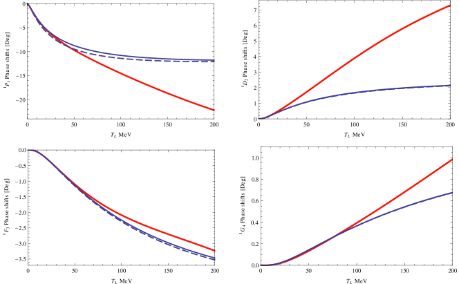
Figure 1: Phase shifts at LO. The dashed and solid blue lines and the solid red line correspond to the Born approximation, the solution to the integral equation and the Nijmegen PWA, respectively.

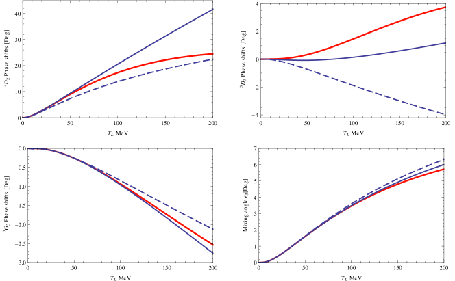
Figure 2: Phase shifts at LO. The dashed and solid blue lines and the solid red line correspond to the Born approximation, the solution to the integral equation and the Nijmegen PWA, respectively.

This work is supported by the EU (HadronPhysics3 project “Study of strongly interacting matter”), the European Research Council (ERC-2010-StG 259218 NuclearEFT) the DFG (GE 2218/2-1) and the Georgian Shota Rustaveli National Science Foundation (grant 11/31).

References

• (1) S. Weinberg, Phys. Lett. B 251, 288 (1990); Nucl. Phys. B363, 3 (1991).
• (2) E. Epelbaum, H. -W. Hammer and U.-G. Meißner, Rev. Mod. Phys.  81, 1773 (2009).
• (3) D. R. Phillips, S. R. Beane and T. D. Cohen, Annals Phys. 263, 255 (1998).
• (4) M. J. Savage, [nucl-th/9804034].
• (5) G. Feinberg and A. Pais, Phys. Rev. 131, 2724 (1963).
• (6) E. Epelbaum and J. Gegelia, Eur. Phys. J. A 41, 341 (2009).
• (7) C. Zeoli, R. Machleidt and D. R. Entem, arXiv:1208.2657 [nucl-th].
• (8) E. Epelbaum and J. Gegelia, Phys. Lett. B 716, 338 (2012).
• (9) S. Weinberg, Phys. Rev.  150, 1313 (1966).
• (10) V. G. Kadyshevsky, Nucl. Phys. B 6, 125 (1968).
• (11) J. Gegelia and G. Japaridze, Phys. Rev. D 60, 114038 (1999).
• (12) G. V. Skornyakov and Ter-Martirosyan, Sov. Phys. JETP 4, 648 (1957).
• (13) P. F. Bedaque, H. W. Hammer and U. van Kolck, Phys. Rev. Lett.  82, 463 (1999).
• (14) T. D. Cohen and J. M. Hansen, Phys. Rev. C 59, 13 (1999) [nucl-th/9808038].
• (15) M. Pavon Valderrama, E. Ruiz Arriola, Phys. Rev. C 72, 044007 (2005).
• (16) J. J. de Swart, et al., nucl-th/9509032.