Thermodynamic Casimir Forces between a Sphere and a Plate: Monte Carlo Simulation of a Spin Model

Abstract

We study the thermodynamic Casimir force between a spherical object and a plate. We consider the bulk universality class of the three-dimensional Ising model, which is relevant for experiments on binary mixtures. To this end, we simulate the improved Blume-Capel model. Following Hucht, we compute the force by integrating energy differences over the inverse temperature. We demonstrate that these energy differences can be computed efficiently by using a particular cluster algorithm. Our numerical results for strongly symmetry breaking boundary conditions are compared with the Derjaguin approximation for small distances and the small sphere expansion for large distances between the sphere and the plate.

I Introduction

In 1978 Fisher and de Gennes FiGe78 realized that when thermal fluctuations are restricted by the finite extension of the system, a force acts on the boundaries. Since this effect is similar to the Casimir effect, where the restriction of quantum fluctuations induces a force, it is called thermodynamic Casimir effect. Recently this force could be detected for various experimental systems and quantitative predictions could be obtained from Monte Carlo simulations of spin models Ga09 . The thermodynamic Casimir force is experimentally and maybe technologically interesting since it depends, in contrast to other forces, strongly on the temperature. Hence, since the temperature can be easily changed in experiments, the thermodynamic Casimir force can be easily manipulated. For a discussion of the thermodynamic Casimir force in the general context of nanoscale science see ref. Frenchetal .

Experiments on thin films of ⁴He and mixtures of ³He and ⁴He near the $\lambda$-transition GaCh99 ; GaCh02 ; GaScGaCh06 and on thin films of binary mixtures near the mixing-demixing transition FuYaPe05 ; RaBoJa07 have been performed. Theoretically these experiments are well described by a plate-plate geometry. For this geometry the thermodynamic Casimir force per area $F_{C}$ follows the finite size scaling form Krech

$$F_{C}\simeq k_{B}TL^{-d}\;\theta(t[L/\xi_{0,+}]^{1/\nu})\;\;,$$ (1)

where $L$ is the thickness of the film, $t$ is the reduced temperature, $d$ is the dimension of the bulk system and $\theta$ is a universal function that depends on the bulk and boundary universality classes that characterize the film. The correlation length in the high temperature phase behaves as $\xi\simeq\xi_{0,+}t^{-\nu}$, where $\xi_{0,+}$ is the amplitude of the correlation length in the high temperature phase and $\nu$ is the critical exponent of the correlation length.

Field theoretic methods do not allow to compute $\theta$ for three-dimensional systems in the full range of the scaling variable Diehl86 ; Diehl97 . Therefore the fact that $\theta$ recently has been computed quite accurately by using Monte Carlo simulations of spin models constitutes valuable progress. In refs. Hucht ; VaGaMaDi08 ; Ha09 ; Ha10 the three-dimensional XY bulk universality class and a vanishing field at the boundary have been studied, which is relevant for the experiments on ⁴He. A quite satisfactory agreement between the experimental results and the theory was found. In refs. DaKr04 ; VaGaMaDi07 ; VaGaMaDi08 ; mybreaking ; PaToDi10 ; mycrossover ; VaMaDi11 ; HuGrSc11 ; mycorrection the Ising bulk universality class and various types of boundary conditions were studied. Note that the mixing-demixing transition of binary mixtures belongs to the Ising bulk universality class.

Experimentally it is easier to access the thermodynamic Casimir force for a sphere-sphere or a sphere-plate than for the plate-plate geometry. Several experiments for these geometries have been performed. In particular, the thermodynamic Casimir force between a colloidal particle immersed in a binary mixture of fluids and the substrate has been directly measured Nature08 ; Gaetal09 . In ref. NeHeBe09 it was demonstrated that the thermodynamic Casimir forces in a colloidal system can be continuously tuned by the choice of the boundary conditions. In addition to homogeneous substrates also chemically patterned ones have been studied So08 ; Tr11 ; Zvyagolskaya . In other experiments, the thermodynamic Casimir force is the driving force for colloidal aggregation, see e.g. refs. Bonnetal09 ; ZvArBe11 .

For simplicity, we restrict the following discussion to the sphere-plate geometry. Furthermore we assume that both the surfaces of the sphere and the plate are homogeneous. In this case, the thermodynamic Casimir force follows the scaling form HaScEiDi98

$$F_{C}(D,R,T)=\frac{k_{B}T}{R}K(t[D/\xi_{0,+}]^{1/\nu},\Delta)$$ (2)

where $R$ is the radius of the sphere, $D$ the distance between the plate and the sphere and $\Delta=D/R$. Note that in the literature often $D/\xi$, where $\xi$ is the bulk correlation length in the high temperature phase, is used instead of $t[D/\xi_{0,+}]^{1/\nu}$ as argument of the universal scaling function. The thermodynamic Casimir force is given by

$$F_{C}(D,R,T)=-k_{B}T\;\frac{\partial F(D,R,T)}{\partial D}\;\;$$ (3)

where $F(D,R,T)$ is the reduced free energy of the system.

In the limit $D\ll R$, the function $K(x,\Delta)$ can be obtained from $\theta(t[L/\xi_{0,+}]^{1/\nu})$ by using the Derjaguin approximation (DA) Derja . Instead, in the limit $D\gg R$ the small sphere expansion BuEi97 can be used. In ref. HaScEiDi98 the function $K$ is discussed for the case where both surfaces strongly adsorb the same component of the binary mixture. The behaviour of $K$ for three-dimensional systems for $D\simeq R$ is inferred from the exactly known one in two dimensions and from mean-field calculations. In ref. troendle the thermodynamic Casimir force is discussed for colloids close to chemically patterned substrates. To this end the authors employ the Derjaguin approximation. They check the range of applicability of the Derjaguin approximation by using mean-field calculations. In section III of troendle , they discuss for a start also homogeneous substrates.

Here we discuss a method to determine the thermodynamic Casimir force for the sphere-plate geometry by using Monte Carlo simulations of spin models. The generalization to the sphere-sphere geometry is straightforward. The method is based on the geometric cluster algorithm of Heringa and Blöte HeBl98 . In the present work, we simulate the improved Blume-Capel model on the simple cubic lattice. We focus on strongly symmetry breaking boundary conditions at the surfaces of the sphere and the plate. We assume that the surface of the plate prefers positive magnetisation. We study the two cases $s_{sphere}=-1$ and $1$, where $s_{sphere}$ is the value of the spins at the surface of the sphere. Preliminary results for $s_{sphere}=0$, indicate that also this case can be efficiently simulated. In our numerical tests we studied spheres of the radii $R=3.5,4.5,7.5$ and $15.5$ lattice spacings. For $R=3.5$ and $4.5$ we considered distances between the sphere and the plate up to $D\approx 10R$. We introduce an effective radius $R_{eff}$ of the sphere which is determined by a particular finite size scaling method. To this end we compute the ratio of partition functions $Z_{-}/Z_{+}$ by using a cluster algorithm which is closely related to the boundary flip algorithm MH93A ; MH93B . The index of $Z$ gives the sign of $s_{sphere}$. In this finite size scaling study we consider $\Delta\approx 25$, which is large compared with the values used otherwise. Analysing our data we find that replacing $R$ by $R_{eff}$ leads to a good scaling behaviour for the whole range of $\Delta$ studied here. As result we obtain reliable estimates for the scaling functions $K_{-}(x,\Delta)$ and $K_{+}(x,\Delta)$ for $1\lessapprox\Delta\lessapprox 12$, where the subscript of $K$ gives the sign of $s_{sphere}$. The most striking observation is that in the low temperature phase $K_{-}(x,\Delta)$ deviates quite strongly from the Derjaguin approximation already for $\Delta\approx 1$ and likely smaller.

The present work should be seen as pilot study that allows for a number of improvements as discussed in section VI. The method discussed here should apply to a broader range of problems as we also shall discuss in section VI.

The paper is organised as follows. First we define the model. Then we discuss the geometry of the systems that we study. In section IV we discuss the algorithm that is used to compute the thermodynamic Casimir force. In section V we present our numerical results. First we discuss the performance of the algorithm. Then we give our results for the scaling functions $K_{\pm}(x,\Delta)$. In section VI we conclude and give an outlook. In Appendix A we discuss the finite size scaling method that we used to determine the effective radius $R_{eff}$.

II The Model

We simulate the Blume-Capel model on the simple cubic lattice. It is defined by the reduced Hamiltonian

$$H=-\beta\sum_{<xy>}s_{x}s_{y}+\tilde{D}\sum_{x}s_{x}^{2}-\tilde{h}\sum_{x}s_{x}\;\;,$$ (4)

where $s_{x}\in\{-1,0,1\}$ and $x=(x_{0},x_{1},x_{2})$ denotes a site on the simple cubic lattice, where $x_{i}$ takes integer values and $<xy>$ is a pair of nearest neighbours on the lattice. The partition function is given by $Z=\sum_{\{s\}}\exp(-H)$, where the sum runs over all spin configurations. The parameter $\tilde{D}$ controls the density of vacancies $s_{x}=0$. In the limit $\tilde{D}\rightarrow-\infty$ vacancies are completely suppressed and hence the spin-1/2 Ising model is recovered. Here we consider a vanishing external field $\tilde{h}=0$ throughout. In $d\geq 2$ dimensions the model undergoes a continuous phase transition for $-\infty\leq\tilde{D}<\tilde{D}_{tri}$ at a $\beta_{c}$ that depends on $\tilde{D}$. For $\tilde{D}>\tilde{D}_{tri}$ the model undergoes a first order phase transition, where $\tilde{D}_{tri}=2.0313(4)$ DeBl04 .

Numerically, using Monte Carlo simulations it has been shown that there is a point $(\tilde{D}^{*},\beta_{c}(\tilde{D}^{*}))$ on the line of second order phase transitions, where the amplitude of leading corrections to scaling vanishes. Our recent estimate is $\tilde{D}^{*}=0.656(20)$ mycritical . In mycritical we simulated the model at $\tilde{D}=0.655$ close to $\beta_{c}$ on lattices of a linear size up to $L=360$. From a standard finite size scaling analysis of phenomenological couplings like the Binder cumulant we find $\beta_{c}(0.655)=0.387721735(25)$. Furthermore the amplitude of leading corrections to scaling is at least by a factor of $30$ smaller than for the spin-1/2 Ising model. In order to set the scale we use the second moment correlation length in the high temperature phase. Its amplitude is given by mycorrection

$$\xi_{2nd,0,+} = 0.2283(1)-1.8\times(\nu-0.63002)+275\times(\beta_{c}-0.387721735)\;\;$$ (5)

$$\mbox{using}\;\;t=\beta_{c}-\beta\;\;\mbox{as definition of the reduced temperature}.$$

In the high temperature phase there is little difference between $\xi_{2nd}$ and the exponential correlation length $\xi_{exp}$ which is defined by the asymptotic decay of the two-point correlation function. Following pisaseries :

$$\lim_{t\searrow 0}\frac{\xi_{exp}}{\xi_{2nd}}=1.000200(3)\;\;$$ (6)

for the thermodynamic limit of the three-dimensional system. Note that in the following $\xi_{0}$ always refers to $\xi_{2nd,0,+}$.

III Geometry of the System

We have used fixed boundary conditions in $0$-direction and periodic boundary conditions in $1$ and $2$ directions. In most of our simulations we have fixed $s_{x}=1$ for $x_{0}=0$ and $x_{0}=L_{0}+1$. In order to check the effect of the second boundary, we have performed some simulations with $s_{x}=1$ for $x_{0}=0$ and $s_{x}=0$ for $x_{0}=L_{0}+1$. In both cases there are $L_{0}$ layers with fluctuating spins. For $i=1,2$ we take $x_{i}=-L_{i}/2+1$,$-L_{i}/2+2$,$...$, $L_{i}/2$ and $L_{1}=L_{2}=L$ throughout.

To model the spherical object, we have fixed all spins $s_{x}$ to $s_{sphere}$ for

$$\sqrt{(x_{0}-h)^{2}+x_{1}^{2}+x_{2}^{2}}\leq R$$ (7)

The distance between the sphere and the plate is given by

$$D=h-R\;\;.$$ (8)

Analysing our data we shall introduce an effective radius $R_{eff}$ of the sphere that we determine by using a finite size scaling analysis in Appendix A below. Taking also into account the extrapolation length $l_{eff}$ at the boundary of the plate we arrive at

$$D_{eff}=h-R_{eff}+l_{eff}$$ (9)

where $l_{eff}=0.96(2)-0.5=0.46(2)$ for the model and boundary conditions discussed here mycrossover . Note that $l_{eff}=0.96(2)$ given in ref. mycrossover refers to $x_{0}=0.5$ as location of the boundary. Mostly we have simulated the two cases $s_{sphere}=-1$ and $1$. In our study, nearest neighbour pairs that contain a fixed and a fluctuating spin are coupled by the same $\beta$ as nearest neighbour pairs that contain two fluctuating spins. One could imagine to chose the couplings depending on the position on the surface of the sphere, in order to effectively improve the spherical shape of the object.

IV The algorithm

In order to determine the thermodynamic Casimir force $F_{C}(D,R,\beta)$, eq. (3), between the plate and the sphere, we compute finite differences of the reduced free energy $F(D,R,\beta)$ of the system

$$-\beta F_{C}(D,R,\beta)\approx\Delta F(D,R,\beta)=F(D+1/2,R,\beta)-F(D-1/2,R,\beta)\;\;.$$ (10)

Note that we chose the difference of the distances equal to one due to the discrete translational invariance of the lattice. Similarly to the proposal of Hucht Hucht , we determine $\Delta F(D,R,\beta)$ by integrating the corresponding difference of energies

$$\Delta F(D,R,\beta)=-\int_{\beta_{0}}^{\beta}\mbox{d}\tilde{\beta}\;\Delta E(D,R,\tilde{\beta})$$ (11)

where $\Delta E(D,R,\beta)=E(D+1/2,R,\beta)-E(D-1/2,R,\beta)$ and

$$E(D,R,\beta)=\left\langle\sum_{<xy>}s_{x}s_{y}\right\rangle_{D,R,\beta}\;\;.$$ (12)

The value of $\beta_{0}$ is chosen such that $\Delta E(D,R,\beta_{0})\approx 0$, which is the case for $D\gg\xi_{bulk}(\beta_{0})$. The integration is done numerically, using the trapezoidal rule. It turns out that similar to the study of the plate-plate geometry $O(100)$ nodes are needed to compute the thermodynamic Casimir force in the whole range of temperatures that is of interest to us.

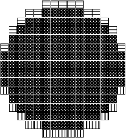
Figure 1: Two-dimensional sketch of two spheres at $x_{0}=D-1/2$ and $D+1/2$. The $0$-axis is drawn in vertical direction. The overlapp of the two spheres is given by black squares with white dots. Sites that only belong to the lower sphere are represented by squares with vertical lines and those that only belong to the upper sphere by squares with horizontal lines.

Routinely one would carry out this programme by simulating the systems for $D-1/2$ and $D+1/2$ separately using standard Monte Carlo algorithms. In order to avoid systematic errors, $L_{0},L\gg D,R$ should be taken. However the variance of $E(D,R,\beta)$ and the CPU-time required for the simulations are increasing with the system size. In fact, first numerical experiments have shown that even for moderate values of $D$ and $R$, this approach fails to give sufficiently accurate results.

The expectation value $<s_{x}s_{y}>$ only differs strongly between the two systems for nearest neighbour pairs $<xy>$ close to the sphere and this difference decays at least power-like with increasing distance from the sphere. Therefore, computing $\Delta E(D,R,\beta)$ one would like to concentrate on the part of the system, where the difference in $<s_{x}s_{y}>$ is large and to avoid to pick up variance from the remainder. Routinely one could implement this idea by ad hoc restricting the range of summation in eq. (12). The problem is that this ad hoc restriction leads to a systematic error that needs to be controlled, e.g. by comparing the results of different restrictions. In the following we shall discuss an algorithm that generates the restriction of the summation to the neighbourhood of the sphere automatically and at the same time allows to compute $\Delta E(D,R,\beta)$ without bias.

This algorithm is closely related to the geometric cluster algorithm HeBl98 . Similar to ref. SwWa86 , two systems are updated jointly. These two systems share the values of $\beta,L_{0},L$ and $R$. The distance of the sphere from the boundary is $D-1/2$ and $D+1/2$ for system 1 and 2, respectively. In the following the spins are denoted by $s_{x,i}$, where the second index indicates whether the spin belongs to system 1 or 2. Configurations are denoted by $\{s\}_{i}$. The combined partition function is given by

$$Z_{com}=\sum_{\{s\}_{1}}\sum_{\{s\}_{2}}\exp\left[-H_{1}(\{s\}_{1})-H_{2}(\{s\}_{2})\right]$$ (13)

where $H_{i}$ is the reduced Hamiltonian of the system $i$. The cluster update comprises the exchange of spins

$$s_{x,1}^{\prime} = s_{x,2}$$

$$s_{x,2}^{\prime} = s_{x,1}$$ (14)

for all sites $x$ in the cluster. Performing this exchange of spins for all sites within a cluster is called flipping the cluster in the following. A cluster is build in the usual way: A pair of nearest neighbours $<xy>$ is deleted with the probability $p_{d}$ and frozen otherwise. In our case HeBl98

$$p_{d}=\mbox{min}\left[1,\exp\left(-\beta[s_{x,1}-s_{x,2}][s_{y,1}-s_{y,2}]\right)\right]\;\;.$$ (15)

Two sites of the lattice belong to the same cluster if they are connected at least by one chain of frozen pairs of nearest neighbours. Various choices of the selection of the clusters to be updated are discussed in the literature. In the case of the Swendsen-Wang SwWa87 algorithm all clusters are constructed and then all spins within a given cluster are flipped with probability $1/2$. In the single cluster algorithm Wolff one first selects randomly one site of the lattice. Then one constructs only the cluster that contains this site. All spins within this cluster are flipped. Further choices have been discussed in the literature Kerler ; wall .

In our case, the choice of the clusters to be flipped is dictated by the requirement that the fixed spins have to keep their value under the update. The exchange of spins should not be allowed for those sites $x$, where $s_{x,1}$ is fixed while $s_{x,2}$ is not, or vice versa. In the following these sites are called frozen sites. In Fig. 1 these sites are represented by squares with vertical or horizontal lines on them. In the following a cluster that contains at least one frozen sites is called frozen cluster. In the update all clusters except for the frozen ones are flipped. In order to perform this operation only the frozen clusters have to be constructed.

Now let us discuss how $\Delta E$, eq. (11), is computed. Let us assume that after equilibration we have generated a sequence of $N+1$ configurations that are labelled by $t$. We get

$$\Delta E\approx\frac{1}{N}\sum_{t=1}^{N}\Delta E_{est,t}\approx\frac{1}{N}\sum_{t=1}^{N}\frac{1}{2}(\Delta E_{est,t}+\Delta E_{est,t+1})$$ (16)

where

$$\Delta E_{est,t}=\sum_{<xy>}\left[s_{x,2}^{(t)}s_{y,2}^{(t)}-s_{x,1}^{(t)}s_{y,1}^{(t)}\right]$$ (17)

is the standard estimator of $\Delta E$. Combining the right hand side of eq. (16) and the particular properties of the update discussed above we arrive at the improved estimator

$$\Delta E_{imp} = \frac{1}{2}\sum_{<xy>}\left([s_{x,2}^{(t)}s_{y,2}^{(t)}-s_{x,1}^{(t)}s_{y,1}^{(t)}]+[s_{x,2}^{(t+1)}s_{y,2}^{(t+1)}-s_{x,1}^{(t+1)}s_{y,1}^{(t+1)}]\right)$$ (18)

$$= \frac{1}{2}\sum_{<xy>}\left([s_{x,2}^{(t)}s_{y,2}^{(t)}-s_{x,1}^{(t+1)}s_{y,1}^{(t+1)}]+[s_{x,2}^{(t+1)}s_{y,2}^{(t+1)}-s_{x,1}^{(t)}s_{y,1}^{(t)}]\right)$$

$$= \frac{1}{2}\sum_{<xy>\in C_{f}}\left([s_{x,2}^{(t)}s_{y,2}^{(t)}-s_{x,1}^{(t+1)}s_{y,1}^{(t+1)}]+[s_{x,2}^{(t+1)}s_{y,2}^{(t+1)}-s_{x,1}^{(t)}s_{y,1}^{(t)}]\right)$$

where $<xy>\in C_{f}$ means that at least one of the sites $x$ or $y$ belongs to a frozen cluster. Note that for our choice of the update

$$s_{x,1}^{(t+1)}s_{y,1}^{(t+1)}=s_{x,2}^{(t)}s_{y,2}^{(t)}\;\;\;\mbox{and}\;\;\;s_{x,2}^{(t+1)}s_{y,2}^{(t+1)}=s_{x,1}^{(t)}s_{y,1}^{(t)}$$ (19)

for all nearest neighbour pairs $<x,y>$ where neither $x$ nor $y$ belongs to a frozen cluster.

Whether we have achieved progress this way depends on the average volume taken by frozen clusters. Our numerical study discussed in detail below shows indeed that for the whole range of $\beta$ the total size of all frozen clusters is small compared with the volume of the lattice. Hence the variance of $\Delta E_{imp}$ is drastically reduced compared with the standard estimator. Furthermore, since the sum runs only over the frozen clusters, the numerical effort to compute $\Delta E_{imp}$ is much smaller than the one to compute the standard estimator.

In the following we shall discuss the details of our implementation. We simulate a large number of distances $D_{min},D_{min}+1,...,D_{max}$ jointly. We perform the exchange cluster update and the measurement of $\Delta E_{imp}$ for all $D_{max}-D_{min}$ pairs $(D_{1},D_{2})$ with $D_{2}-D_{1}=1$. In our C-program we store the spins in the array int spins[I_D][L_0][L][L]; where I_D equals the number of distances $D_{max}-D_{min}+1$ that are simulated. Routinely one would swap the spins stored in spins[i_c][i_0][i_1][i_2] and spins[i_c+1][i_0][i_1][i_2], where the site represented by [i_0][i_1][i_2] is not a member of a frozen cluster. Instead, in order to save CPU time, we do that for the sites that belong to frozen clusters. This way, the systems with the distances $D_{1}$ and $D_{2}$ of the sphere from the plate interchange their position in the array spins. In order to keep track of where the systems are stored in the array spins, we introduce the array int posi[I_D]; where the index i_d equals $D-D_{min}$ and posi[i_d] indicates where the system with the distance $D$ of the sphere from the plate is stored in spins. Note that parallel tempering simulations are usually organized in a similar way. Instead of swapping configurations, the location of the systems with the temperatures $T_{i}$ and $T_{i+1}$ is interchanged.

In order to get an ergodic algorithm we supplement the exchange cluster algorithm discussed above with standard updates of the individual systems. To this end we perform Swendsen-Wang SwWa87 updates and heat-bath updates. In case of the Swendsen-Wang cluster-update we keep the clusters that contain fixed spins fixed. Those clusters that do not contain fixed spins are flipped with probability $1/2$.

These updates are performed in a fixed sequence: First we sweep once for each systems over the whole lattice using the heat-bath algorithm. It follows one Swendsen-Wang cluster-update for each system. Then we perform $i_{m}$-times the following two steps:

• For $D=D_{min},...,$ up to $D_{max}-1$ perform in a sequence the exchange cluster update and the measurement of $\Delta E_{imp}$ for the pairs of distances $D$ and $D+1$.

• Perform for each system one sweep with the heat-bath algorithm over a sub-lattice characterized by $x_{0}\leq l_{0}$, $-l_{1}/2\leq x_{1}\leq l_{1}/2$ and $-l_{2}/2\leq x_{2}\leq l_{2}/2$.

In the following we shall denote this sequence of updates as one cycle of the algorithm. Since the estimator $\Delta E_{imp}$ takes mainly data from the neighbourhood of the sphere, it seems useful to perform additional updates in this region of the lattice. Therefore we introduced the heat-bath updates of the sub-lattice. Here we made no attempt to optimize the shape and size of this sub-lattice nor the frequency of these updates.

V Numerical Results

As a first test of our implementation we simulated systems with the radius $R=2.5$ and lattices of the size $28\times 16^{2}$ and $38\times 20^{2}$. We considered the distances $1.5\leq D\leq 9.5$ between the sphere and the plate. We fixed $s_{x}=1$ for $x_{0}=0$ and $x_{0}=L_{0}+1$. We simulated both $s_{sphere}=-1$ and $+1$ at the two values $\beta=0.387$ and $0.389$ of the inverse temperature. We simulated with the exchange cluster algorithm and without. For these lattice sizes we still get differences of the energies $\Delta E$ that are clearly larger than the statistical error from simulations that take about one day of CPU-time on a single core of the CPU in the standard way. Our results with and without the exchange cluster algorithm are compatible within the statistical errors. But even for the small lattices sizes used here, the statistical error, using an equal amount of CPU-time, is reduced by more than a factor of 10 by using the exchange cluster algorithm and the improved estimator (18). After these preliminary studies were concluded successfully, we performed an extensive study aiming at physically relevant results. First we summarize the parameters of our simulations. Then we discuss the performance of the algorithm, focussing on the size $N_{clu}$ of the frozen clusters minus the number of fixed spins. Finally we present our results for the thermodynamic Casimir force and compare them with the literature.

V.1 Our simulations

We studied spheres of the radii $R=3.5$, $4.5$ and $7.5$ for both $s_{sphere}=-1$ and $1$ and $R=15.5$ for $s_{sphere}=1$ only. For these radii, we simulated systems with $1.5\leq D\leq D_{max}$, where $D_{max}=16.5$, $40.5$, $32.5$, and $10.5$ for $R=3.5$, $4.5$, $7.5$ and $15.5$, respectively. In the following we shall denote the number of values of $D$ by $I_{D}$. We simulated these systems for about 100 values of $\beta$. We adapted the step-size in $\beta$. Close to $\beta_{c}$, the step-size is the smallest. For all values of $\beta$ we simulated lattices of the size $148\times 80^{2}$, $298\times 100^{2}$, $298\times 160^{2}$ and $398\times 200^{2}$, respectively. In the case of these simulations, we fixed $s_{x}=1$ for $x_{0}=0$ and $x_{0}=L_{0}+1$. We fixed the parameter of the update cycle to $i_{m}=20I_{D}$. The sizes of the sub-lattice that is updated in excess $i_{m}$ times per cycle using the heat-bath algorithm is $28\times 16^{2}$, $55\times 20^{2}$, $56\times 32^{2}$ and $58\times 64^{2}$ for $R=3.5$, $4.5$, $7.5$ and $15.5$, respectively. These parameters are chosen ad hoc. For lack of human time we did not try to optimize them.

In order to check for the effect of the finite values of $L_{0}$ and $L$, we redid the simulations for $R=3.5$ in the neighbourhood of $\beta_{c}$ on lattices of the sizes $198\times 120^{2}$ and $298\times 200^{2}$, where we considered both $s_{x}=0$ and $s_{x}=1$ for $x_{0}=L_{0}+1$. For $R=4.5$ we simulated in addition lattices of the size $398\times 150^{2}$ with $s_{x}=0$ for $x_{0}=L_{0}+1$ and $448\times 150^{2}$ with $s_{x}=1$ for $x_{0}=L_{0}+1$ in the neighbourhood of $\beta_{c}$. For these additional simulations we chose $i_{m}=10I_{D}$. The sizes of the sub-lattice that is updated in excess are the same as above. In order to keep the figures readable we shall give in sections V.3, V.4 and V.5 below results for $s_{x}=1$ at $x_{0}=L_{0}+1$ only. The results obtained for $s_{x}=0$ at $x_{0}=L_{0}+1$ confirm our final conclusions.

Focussing on larger distances we simulated $R=3.5$ for $25.5\leq D\leq 32.5$. For $s_{sphere}=-1$ in the range $0.3864\leq\beta\leq 0.3888$ and for $s_{sphere}=1$ in the range $0.3864\leq\beta\leq 0.3892$ we simulated a lattice of the size $598\times 200^{2}$. The size of the sub-lattice that is updated in excess $i_{m}$ times per cycle using the heat-bath algorithm is $43\times 16^{2}$. For $\beta$ less close to $\beta_{c}$ we simulated smaller lattices. For these simulations we took $i_{m}=20I_{D}$. Finally we performed simulations for $R=4.5$ at the distances $31.5\leq D\leq 40.5$ using a lattice of the size $598\times 200^{2}$ in the range $0.386\leq\beta\leq 0.3886$ also taking $i_{m}=20I_{D}$.

For each of these simulations we performed $10^{4}$ up to $2\times 10^{4}$ update cycles. For $s_{sphere}=0$ and $R=3.5$, $4.5$, and $7.5$ we simulated at $\beta_{c}$ only. In all our simulations we used the Mersenne twister algorithm twister as pseudo-random number generator. Our code is written in C and we used the Intel compiler. Simulating at $\beta=\beta_{c}$, our Swenden-Wang update takes about $1.1\times 10^{-7}$ s and the local heat-bath update about $3.5\times 10^{-8}$ s per site on a single core of a Quad-Core AMD Opteron(tm) 2378 CPU. The exchange cluster, including the measurement (18) takes roughly $2.6\times 10^{-7}$ s per site of the frozen clusters. In total our simulations took roughly the equivalent of 50 years of CPU time on one core of a Quad-Core AMD Opteron(tm) 2378 CPU.

V.2 Size of the frozen clusters

The CPU-time needed for one update cycle depends on the size of the frozen clusters. Also the variance of the estimator (18) compared with the standard one can be small only if the size of the frozen clusters is small compared with the volume of the lattice. Therefore we shall discuss the size of the frozen clusters and its dependence on the parameters $\beta$, $R$, $D$ and the lattice size in some detail below.

To give a first impression, we plot

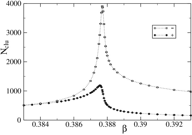
Figure 2: We plot the average size $N_{clu}$ of the frozen clusters minus the number of frozen sites for the radius $R=7.5$ and the distance $D=32$ as a function of the inverse temperature $\beta$. The upper and the lower curve represent the results for $s_{sphere}=-1$ and $1$, respectively.

in Fig. 2 the average size $N_{clu}$ of the frozen clusters minus the number of frozen sites for the radius $R=7.5$ and the distance $D=32$, i.e. for the pair of systems with $D=31.5$ and $32.5$, for $s_{sphere}=-1$ and $1$. For decreasing $\beta$ in the high temperature phase, the average size of the frozen clusters for $s_{sphere}=-1$ and $1$ seems to become identical. As the critical point is approached, the size for $s_{sphere}=-1$ becomes clearly larger than for $s_{sphere}=1$. This remains true in the low temperature phase. In both cases, the maximum $N_{clu,max}$ is located close to $\beta_{c}$. We find $N_{clu,max}\approx 3900$ and $N_{clu,max}\approx 1190$ for $s_{sphere}=-1$ and $1$, respectively. Note that this is only a small fraction of the total volume of the lattice, $298\times 160^{2}=7628800$.

Let us now discuss the behaviour of $N_{clu}$ in more detail. Since $p_{d}=1$ for $\beta=0$, the frozen clusters consist of the frozen sites only, i.e. $N_{clu}=0$. At low temperatures, the configurations become ordered. Therefore also in this limit the frozen clusters consist of the frozen sites only.

From our numerical data we see that for fixed $\beta$ and lattice size, $N_{clu}$ is monotonically increasing with increasing distance $D$. For $L_{0},L,D\gg\xi$, $N_{clu}$ seems to converge to a finite value $N_{clu,\infty}$. In the high temperature phase, $\beta<\beta_{c}$, this value is the same for $s_{sphere}=-1$ and $1$. We fitted our data in the high temperature phase with the Ansatz $N_{clu,\infty}=c(\beta_{c}-\beta)^{-y}$. For $R=3.5$ we get quite reasonable fits with the result $y\approx 0.6$. Fits for larger radii, where we have less data apparently give smaller values of $y$. However, since $N_{clu,\infty}$ should increase with increasing radius $R$, this observation seems to be an artifact of our finite data set. A theoretical understanding of the behaviour of $N_{clu,\infty}$, relating $y$ with known critical exponents, analogous to ref. HeBl98 , would be desirable.

Next let us study the dependence of $N_{clu}$ on the linear lattice sizes $L_{0}$ and $L$ in the

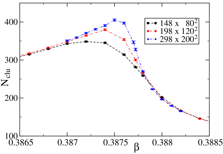
Figure 3: We plot $N_{clu}$ as a function of $\beta$ for $R=3.5$, $D=16$ and $s_{sphere}=1$ focussing on the neighbourhood of the critical point. We give results for the lattices sizes $148\times 80^{2}$, $198\times 120^{2}$ and $298\times 200^{2}$.

neighbourhood of the critical point. In Fig. 3 we plot $N_{clu}$ as a function of $\beta$ for $R=3.5$, $D=16$ and $s_{sphere}=1$ for the lattice sizes $148\times 80^{2}$, $198\times 120^{2}$ and $298\times 200^{2}$. For $\beta\lessapprox 0.387$ and $\beta\gtrapprox 0.3882$ the estimates of $N_{clu}$ for the different lattice sizes are consistent within the statistical error. Instead for $0.387\lessapprox\beta\lessapprox 0.3882$ a dependence of $N_{clu}$ on the lattice size can be seen. For most values of $\beta$ in this range $N_{clu}$ is increasing with increasing lattice size. However for $\beta\approx 0.388$ the value of $N_{clu}$ for $148\times 80^{2}$ seems to be a bit larger than those for the lattices sizes $198\times 120^{2}$ and $298\times 200^{2}$. For $s_{sphere}=-1$ we get a qualitatively similar behaviour. The same holds for $R=4.5$ for both $s_{sphere}=-1$ and $1$.

Finally let us discuss the behaviour of $N_{clu}$ at the critical point in more detail. In Fig. 4 we plot $N_{clu}$ as a function of $D$

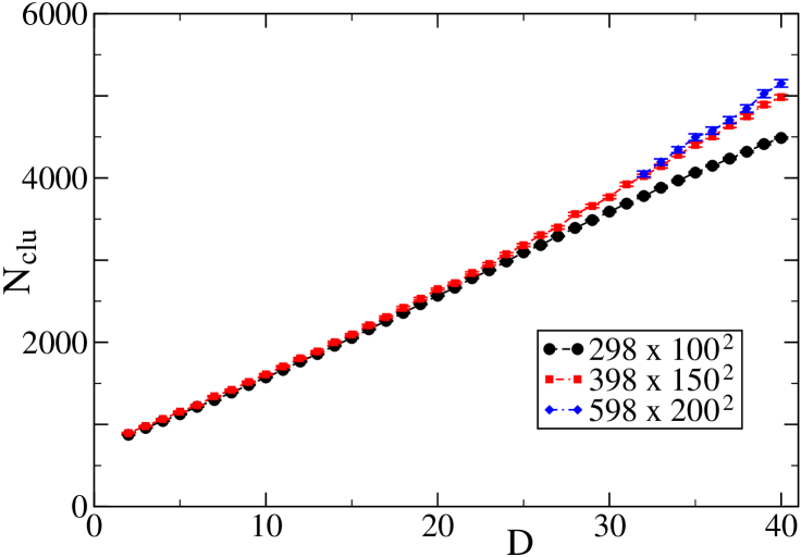
Figure 4: We plot $N_{clu}$ as a function of $D$ for $R=4.5$, $s_{sphere}=-1$ and $\beta=\beta_{c}$. We give results for the lattice sizes $298\times 100^{2}$, $448\times 150^{2}$ and $598\times 200^{2}$.

for $R=4.5$, $s_{sphere}=-1$ and $\beta=\beta_{c}$. The value of $N_{clu}$ seems to increase somewhat faster than linearly with the distance $D$. Differences between the results for the lattice sizes $298\times 100^{2}$, $448\times 150^{2}$ and $598\times 200^{2}$ are clearly visible. Similar observations can be made for $s_{sphere}=1$ and also for other radii.

In table 1 we give $N_{clu}$ at $\beta_{c}$ for the radii $R=3.5$, $4.5$ and $7.5$ for

Table 1: $N_{clu}$ for $s_{sphere}=-1$, $0$ and $1$ at the critical point for $D\approx 4.3R$. The results are taken from the lattice sizes $148\times 80^{2}$, $298\times 100^{2}$, $298\times 160^{2}$ for $R=3.5$, $4.5$ and $7.5$, respectively.

$R$ $\diagdown$ $s_{sphere}$	$-1$	$0$	$1$
3.5	1096(3)	1495(5)	269(1)
4.5	2464(6)	04201(19)	565(2)
7.5	3862(8)	11203(67)	970(2)

the distance $D\approx 4.3R$, i.e. $D=15$, $19$, and $32$, respectively. As one might expect, $N_{clu}$ is increasing with increasing radius $R$. The ratio of $N_{clu}$ for $s_{sphere}=-1$ and $s_{sphere}=1$ is roughly the same for all three radii. In contrast, we find that $N_{clu}$ is increasing more rapidly with increasing $R$ for $s_{sphere}=0$ than for $s_{sphere}=\pm 1$. For $s_{sphere}=\pm 1$ the results for $R=4.5$ and $7.5$ suggest that $N_{clu}$ is increasing less than linearly with the radius $R$, while the opposite seems to be true for $s_{sphere}=0$.

In section IV we argued that the estimator (18) reduces the variance if $N_{clu}\ll L_{0}\times L^{2}$. For $s_{sphere}=\pm 1$ we have verified that this is indeed the case for the full range of $\beta$ and all radii and lattice sizes studied here. Our preliminary results for $s_{sphere}=0$ obtained at $\beta_{c}$ indicate that in this case the exchange cluster algorithm is less efficient than for $s_{sphere}=\pm 1$. Still it seems plausible that also for $s_{sphere}=0$ meaningful results for the thermodynamic Casimir force can be obtained.

V.3 The thermodynamic Casimir force: Effects of the finite lattice

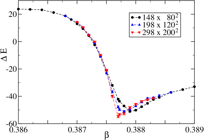
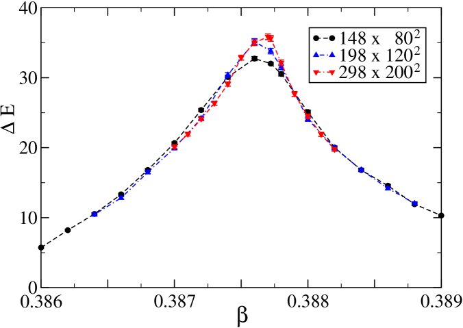
Figure 5: We plot $\Delta E$ as a function of $\beta$ for $R=3.5$ and $D=16$. The lattice sizes are $148\times 80^{2}$, $198\times 120^{2}$, and $298\times 200^{2}$. In the upper and the lower part of the figure we give results for $s_{sphere}=-1$ and $s_{sphere}=1$, respectively.

For $\beta\neq\beta_{c}$ corrections to the limit $L_{0},L\rightarrow\infty$ decay exponentially with increasing lattice size. Therefore corrections should be negligible for $L_{0},L\gg\xi_{bulk}$. Instead, at the critical point, we expect that corrections decay power-like. For $R=3.5$ we checked explicitly how $\Delta E$ depends on the lattice size. To this end we simulated in the neighbourhood of $\beta_{c}$ in addition to the lattice of the size $148\times 80^{2}$ ones of the sizes $198\times 120^{2}$ and $298\times 200^{2}$. In Fig. 5 we plot for $D=16$ our results for the difference of energies $\Delta E$ as a function of $\beta$. We give our results for $s_{sphere}=-1$ and $1$ in the upper and the low part of Fig. 5, respectively. We see differences between the results obtained for the $148\times 80^{2}$ and the larger lattices that are statistically significant for $0.3868\lessapprox\beta\lessapprox 0.3886$ and $0.3868\lessapprox\beta\lessapprox 0.3882$ for $s_{sphere}=-1$ and $1$, respectively. Note that $\xi_{bulk}(0.3868)\approx 18.66$, using eq. (5).

In Fig. 6 we give the numerical results of $-\Delta F$

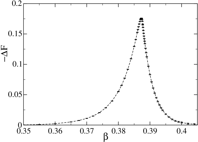
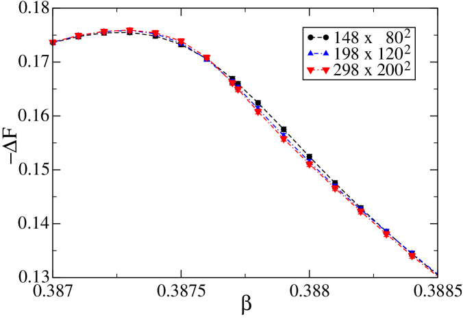
Figure 6: We plot $-\Delta F$ as a function of $\beta$ for $R=3.5$, $D=16$, and $s_{sphere}=-1$. In the upper part of the figure we give the result obtained by using a $148\times 80^{2}$ lattice for the full range of $\beta$ that we consider. In the lower part of the figure we focus on the neighbourhood of $\beta_{c}$, plotting the results for the lattice sizes $148\times 80^{2}$, $198\times 120^{2}$, and $298\times 200^{2}$.

for $R=3.5$, $D=16$ and $s_{sphere}=-1$. In the upper part of the figure we give the result of the numerical integration of $\Delta E$ obtained by using the data for the $148\times 80^{2}$ lattice. In the lower part of the figure we focus on the neighbourhood of $\beta_{c}$, where effects due to finite $L_{0}$ and $L$ become important. As check, we computed $-\Delta F$ in an alternative way: We replaced the estimates of $\Delta E$ from the $148\times 80^{2}$ lattice, where available, by those from the $198\times 120^{2}$ or the $298\times 200^{2}$ lattice. We find that the behaviour of $-\Delta F$ is changed only little. The difference between these results is of a similar size as the statistical error. Note that the statistical error of $-\Delta F$ is the accumulated error of $\Delta E$ over the range of the integration.

We conclude that in a neighbourhood of the critical point the effect of the finite lattice size on $\Delta E$ is clearly visible. However, since the range of $\beta$ where this is the case, is quite small, $-\Delta F$ is affected less. The amplitude of this effect can be estimated by comparing the results obtained for different lattice sizes.

V.4 The scaling function $K_{+}(x,\Delta)$ for $s_{sphere}=1$

In this section we discuss our results for the scaling function $K_{+}(x,\Delta)$ for $s_{sphere}=1$. In a first step we check how well our results obtained for different radii collapse on a single curve. To this end we make use of the effective radius determined in Appendix A, see table 5, and the effective distance (9). In particular $\Delta=D_{eff}/R_{eff}$ in the following analysis of our data. In the plots given below we show the statistical error of the data only. The uncertainty of $D_{eff}$ and $R_{eff}$ still comes on top of this. Essentially it is a two percent uncertainty of the scales.

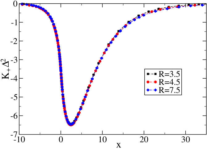
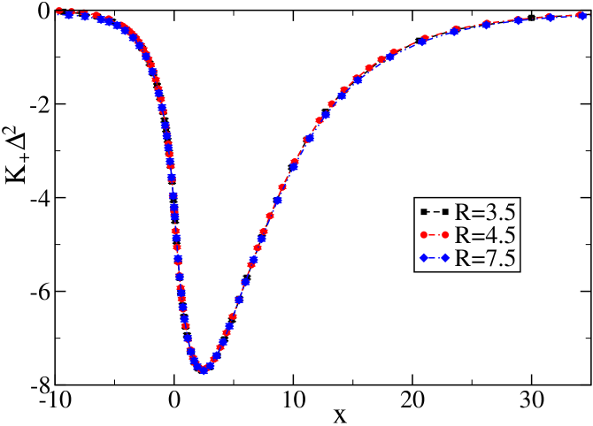
Figure 7: We plot $-R_{eff}\Delta F\Delta^{2}$ as a function of $x=t[D_{eff}/\xi_{0}]^{1/\nu}$ for $s_{sphere}=1$ and the radii $R=3.5$, $4.5$ and $R=7.5$. In the upper part we give results for $\Delta\approx 2.7$, which means $D=6$, $9$ and $18$ for $R=3.5$, $4.5$ and $7.5$, respectively. In the lower part we give results for $\Delta\approx 4.8$, which means $D=12$, $17$ and $32$ for $R=3.5$, $4.5$ and $7.5$, respectively. Note that $\Delta=D_{eff}/R_{eff}$ is used.

In figure 7 we plot $-R_{eff}\Delta F\Delta^{2}$ as a function of $x=t[D_{eff}/\xi_{0}]^{1/\nu}$ for $\Delta\approx 2.7$ and $4.8$. We multiplied by $\Delta^{2}$ to reduce the dependence on $\Delta$. Note that for small values of $\Delta$, $K(0,\Delta)\propto\Delta^{-2}$ and large ones $K(0,\Delta)\propto\Delta^{-\beta/\nu-1}$ HaScEiDi98 ; BuEi97 , where $\beta/\nu=(1+\eta)/2$ and $\eta=0.03627(10)$ mycritical . We took the data obtained by using $148\times 80^{2}$, $298\times 100^{2}$ and $298\times 160^{2}$ lattices for the radii $R=3.5$, $4.5$ and $7.5$, respectively. For this choice $L/R$ is roughly the same for the three radii considered.

In particular for $\Delta\approx 4.8$ we see an excellent collapse of the data obtained for the three different radii. Note that things look far worse when $R$ and $D$ are used instead of $R_{eff}$ and $D_{eff}$. For $\Delta\approx 2.7$ the collapse of the data is slightly worse than for $\Delta\approx 4.8$. In particular for $x\gtrapprox 10$ we see some deviation of the result for $R=3.5$ from that for the two other radii. This is not too surprising, since $\Delta\approx 2.7$ means $D=6$ for $R=3.5$ and also the values of $\beta$ that correspond to $x\gtrapprox 10$ are far from $\beta_{c}$.

We conclude that the data scale well and our numerical results should describe the scaling limit. At the level of our accuracy, one should interpret data obtained for $D\lessapprox 6$ with caution.

In Fig. 8 we plot $K_{+}(x,\Delta)\Delta^{2}$ as a function of $x=t[D/\xi_{0}]^{1/\nu}$ for various values of $\Delta$ in the range $0.75\leq\Delta\leq 10.89$. For each value of $\Delta$, we took the largest radius, where data are available.

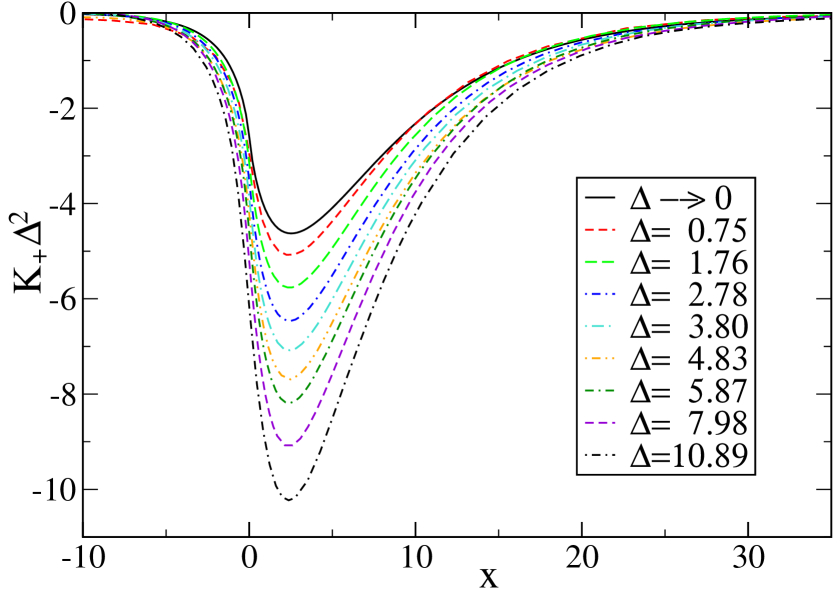
Figure 8: We plot $K_{+}(x,\Delta)\Delta^{2}$ as a function of $x$ for various values of $\Delta$. Note that the index of $K$ indicates $s_{sphere}=1$. We compare the Derjaguin approximation in the limit $\Delta\rightarrow 0$ with our Monte Carlo data for various finite values of $\Delta$. In particular we have used our data for $R=15.5$ and $D=10$ giving $\Delta\approx 0.75$, $R=7.5$ and $D=11$, $18$, $25$, and $32$ giving $\Delta\approx 1.76$, $2.78$, $3.80$, and $4.83$, respectively, and $R=4.5$ and $D=21$, $29$ and $40$ giving $\Delta\approx 5.87$, $7.98$, and $10.89$, respectively.

For comparison we plotted the Derjaguin approximation in the limit $\Delta\rightarrow 0$. For a brief discussion of the Derjaguin approximation see e.g. ref. HaScEiDi98 . As input we used the results for $\theta_{++}(x)$ and $\theta_{+-}(x)$ obtained in ref. mycorrection .

We find that the shape of $K_{+}(x,\Delta)\Delta^{2}$ changes only little with varying $\Delta$. In particular the location of the minimum changes very little with varying $\Delta$. The absolute value of $K_{+}(x,\Delta)\Delta^{2}$ is increasing with increasing $\Delta$, which is consistent with the fact that for large $\Delta$, $K_{+}(0,\Delta)\propto\Delta^{-\beta/\nu-1}$ BuEi97 . These observations are fully consistent with those of ref. troendle . In Fig. 2 a of troendle $K_{(\pm,-)}(\theta,\Delta)/|K_{(\pm,-)}(0,\Delta)|$ is plotted as a function of $\theta=\mbox{sign}(t)D/\xi$. Note that the index $(-,-)$ corresponds to our $+$ and $(+,-)$ to our $-$. For $(-,-)$, the mean-field result for $\Delta=1/3$ is fully consistent with the Derjaguin approximation for four dimensions, while for $\Delta=1$ a small deviation can be seen.

In the following we study in more detail how the minimum of $K_{+}(x,\Delta)$ as function of $x$ depends on $\Delta$. Fortunately, $x_{min}$ is large enough, such that finite $L_{0}$ and $L$ effects are well under control. We located the minimum of $-\Delta F$ by finding the zero of $\Delta E$. To this end, we interpolated $\Delta E$ linearly in $\beta$. Using these results, we computed $x_{min}=(\beta_{c}-\beta_{min})[D_{eff}/\xi_{0}]^{1/\nu}$. In Fig. 9 we plot $x_{min}$ as a function of $\Delta$ using our data obtained for the radii $R=3.5$, $4.5$, $7.5$ and $15.5$. We see that for $\Delta\gtrapprox 2$ the results obtained for different radii agree quite nicely. At $\Delta=2$ the estimate $x_{min}\approx 2.43$ seems plausible. With further increasing $\Delta$ the value of $x_{min}$ is slightly decreasing. For $\Delta\approx 12$ we get $x_{min}\approx 2.3$. For $\Delta\lessapprox 2$ clear deviations between the results obtained by using different radii $R$ can be observed. Therefore we abstain to give a conclusion for the scaling limit in this range. Note that the Derjaguin approximation gives $x_{min}\approx 2.52$ for the limit $\Delta\rightarrow 0$. The Derjaguin approximation predicts that $x_{min}$ is increasing with increasing distance $\Delta$. If that prediction is correct, $x_{min}$ should show a maximum in the interval $0<\Delta\lessapprox 1$.

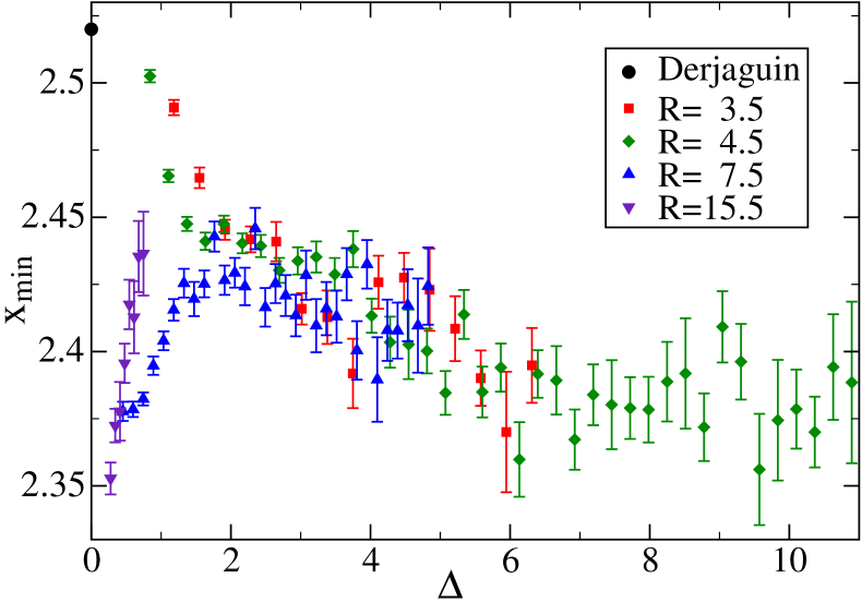
Figure 9: We plot our estimates of $x_{min}$ as a function of $\Delta$. Monte Carlo results obtained by using $R=3.5$, $4.5$, $7.5$ and $15.5$ are given. These are compared with the Derjaguin approximation in the limit $\Delta\rightarrow 0$. Note that $s_{sphere}=1$.

Our results can be compared with the upper part of FIG. 2 of ref. HaScEiDi98 . Note that the authors of ref. HaScEiDi98 consider $D/\xi\simeq x^{\nu}$ as variable. They obtain $x_{min}=1.6^{1/0.63002}=2.1...$ for $\Delta=0$ using the Derjaguin approximation. This discrepancy should be due to the different numerical estimates of the scaling function $\theta_{++}$ of the plate-plate geometry. E.g. following FIG 3 of ref. HaScEiDi98 $\theta_{++}(0)=-0.326$, while our present estimate is $\theta_{++}(0)=-0.410(8)$ mycorrection . Then, according to ref. HaScEiDi98 $x_{min}$ increases and reaches a maximum at $\Delta\approx 3$ assuming the value $x_{min}\approx 2.5^{1/0.63002}\approx 4.3$. Then, with increasing $\Delta$ it is decreasing and reaches $x_{min}\approx 1.5^{1/0.63002}\approx 1.9$ in the limit $\Delta\rightarrow\infty$. In particular for the value assumed at $\Delta\approx 3$ we see a clear discrepancy with our results. It is beyond the scope of the present work to discuss the reliability of the first order $\epsilon$-expansion that has been used in ref. HaScEiDi98 to get the small-sphere expansion.

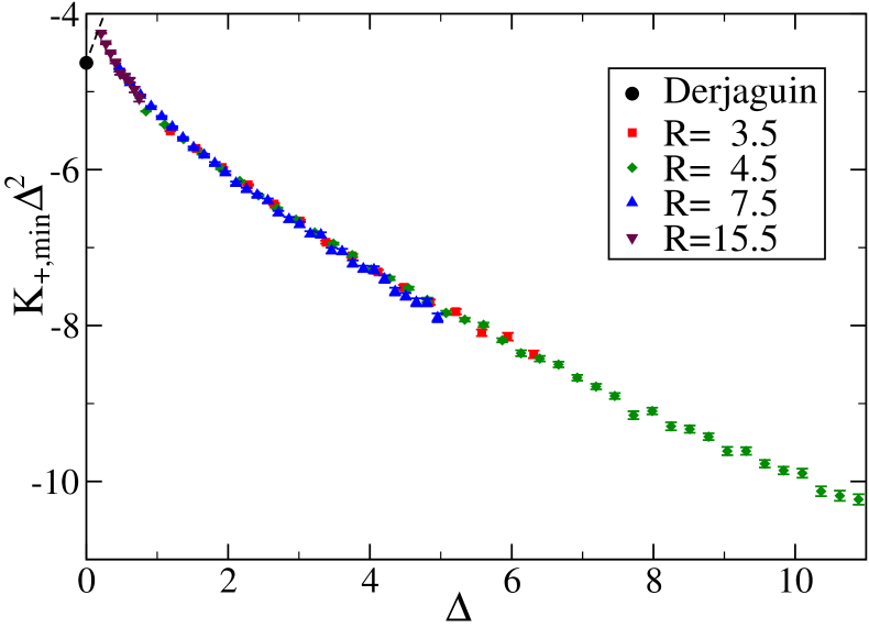
Figure 10: We plot our estimates of $K_{+}(x_{min},\Delta)\Delta^{2}$ as a function of $\Delta$. Monte Carlo results obtained by using $R=3.5$, $4.5$, $7.5$ and $15.5$ are given. The Derjaguin approximation in the limit $\Delta\rightarrow 0$ is given by a black circle. The Derjaguin approximation for finite values of $\Delta$ is represented by a dashed black line. Note that $s_{sphere}=1$.

In Fig. 10 we plot $K_{+}(x_{min},\Delta)\Delta^{2}$ as a function of $\Delta$. We find a nice collapse of the data obtained from different radii of the sphere. In contrast to $x_{min}$, this is also the case for $\Delta\lessapprox 2$. Taking into account our Monte Carlo data only, $K_{+}(x_{min},\Delta)\Delta^{2}$ seems to be a monotonically decreasing function of $\Delta$. However we note that for $\Delta\lessapprox 0.4$ our numerical estimates of $K_{+}(x_{min},\Delta)\Delta^{2}$ are overshooting $\lim_{\Delta\rightarrow 0}K_{+}(x_{min},\Delta)\Delta^{2}\approx-4.63$ obtained from the Derjaguin approximation. Also note that the Derjaguin approximation predicts that $K_{+}(x_{min},\Delta)\Delta^{2}$ increases with increasing $\Delta$, which is indicated by a dashed black line in Fig. 10. Therefore $K_{+}(x_{min},\Delta)\Delta^{2}$ should show a maximum in the interval $0<\Delta\lessapprox 0.4$. In the lower part of Fig. 2. of ref. HaScEiDi98 $K_{+}(x_{min},\Delta)\Delta^{1+\beta/\nu}$ is shown as a function of $\Delta$. For $\Delta\approx 10$ it shows a maximum (minimum with the sign of ref. HaScEiDi98 ) taking a value slightly larger than $-3$. Taking our Monte Carlo data, $K_{+}(x_{min},\Delta)\Delta^{1+\beta/\nu}$ is still slightly increasing at $\Delta\approx 10$ and takes the value $\approx-3.25$.

Finally we discuss the scaling function at the critical point, i.e. $x=0$. In figure 11 we plot our numerical results for $K_{+}(0,\Delta)\Delta^{2}$ as a function of $\Delta$. At the critical point we have to consider finite $L$ and $L_{0}$ effects. Therefore, for $R=4.5$ we plotted our results obtained by using lattices of the sizes $298\times 100^{2}$, $448\times 150^{2}$ and $598\times 200^{2}$. In particular for large $\Delta$ we see a clear deviation of the results obtained for the $298\times 100^{2}$ lattice from the other two. On the other hand the estimates obtained for the $448\times 150^{2}$ and $598\times 200^{2}$ lattices are consistent within the statistical error. Therefore deviations from the $L_{0},L\rightarrow\infty$ limit should be of similar size as the statistical error. In the case of $R=3.5$ we plot the data for the largest lattice size available. We find a quite good collapse of the data obtained for different radii. For $\Delta=1$ we get $K_{+}(0,\Delta)\Delta^{2}\approx-2.8$. We see that $K_{+}(0,\Delta)\Delta^{2}$ is almost linearly decreasing with increasing $\Delta$. For $\Delta=11$ we read off $K_{+}(0,\Delta)\Delta^{2}\approx-6$. The last three data points for $R=3.5$ seem to suggest that $K_{+}(0,\Delta)\Delta^{2}$ is increasing again for $\Delta\gtrapprox 11$. However this is not statistically significant and is likely an artifact.

Using the Derjaguin approximation, we get $\lim_{\Delta\rightarrow 0}K_{+}(0,\Delta)\Delta^{2}\approx-2.59$ and as for $K_{+,min}$, $K_{+}(0,\Delta)\Delta^{2}$ is increasing with increasing $\Delta$. Therefore it seems plausible that $K_{+}(0,\Delta)\Delta^{2}$ has a maximum in the range $0<\Delta\lessapprox 1$.

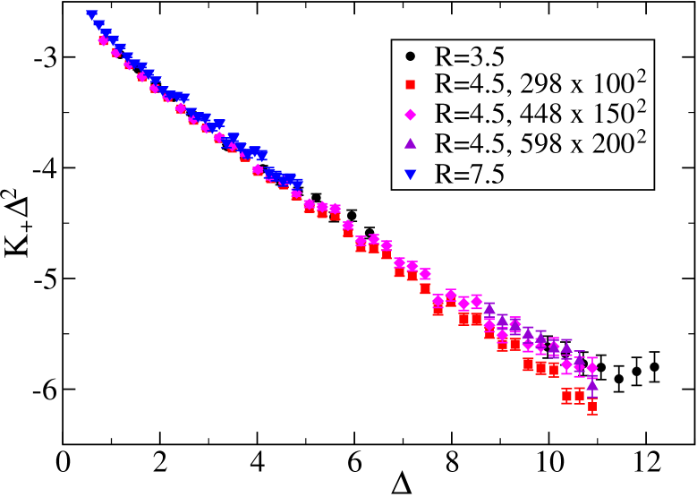
Figure 11: We plot $K_{+}(0,\Delta)\Delta^{2}$ as a function of $\Delta$. Monte Carlo data obtained by using $R=3.5$, $4.5$, and $7.5$ are given. In the case of $R=4.5$ we compare results obtained by using the lattice sizes $298\times 100^{2}$, $448\times 150^{2}$, and $598\times 200^{2}$. Note that $s_{sphere}=1$.

V.5 The scaling function $K_{-}(x,\Delta)$ for $s_{sphere}=-1$

Next let us turn to the scaling function $K_{-}(x,\Delta)$ for $s_{sphere}=-1$. In figure 12 we plot $K_{-}(x,\Delta)\Delta^{2}$ as a function of $x$ for $\Delta\rightarrow 0$ and $\Delta\approx 1$. The limit $\Delta\rightarrow 0$ is obtained by using the Derjaguin approximation. Unfortunately we do not have data for the scaling function $\theta_{+-}(x)$ for the plate-plate geometry for $x\lessapprox-48$ and the amplitude of $\theta_{+-}(x)$ in this range is still significant. Therefore we have extrapolated $\theta_{+-}(x)$ in two different ways: (1) $\theta_{+-}(x)=const$ for $x\lessapprox-48$ and (2) $\theta_{+-}(x)$ is linear in the interval $-65<x<-48$ and $\theta_{+-}(-48)=0.8$, $\theta_{+-}(-65)=0$, for $x<-65$ we take $\theta_{+-}(x)=0$. The true $\theta_{+-}(x)$ should be enclosed by these two extrapolations. In figure 12, the results based on these two extrapolations are denoted by Derjaguin 1 and Derjaguin 2, respectively. For comparison we plot our Monte Carlo result obtained for $R=7.5$ and $D=6$ which corresponds to $\Delta\approx 1$. We observe that the two curves are very similar in the high temperature phase. Since $\theta_{+-}(x)$ has its maximum in the low temperature phase, the same holds for $K_{-}(x,\Delta)$ computed by using the Derjaguin approximation. In contrast, for $\Delta\approx 1$ we find that the maximum is located in the high temperature phase, even though very close to the critical point. Furthermore, $K_{-}(x,\Delta)\Delta^{2}$ at $\Delta\approx 1$ is much smaller than $\lim_{\Delta\rightarrow 0}K_{-}(x,\Delta)\Delta^{2}$ in the low temperature phase. Also the decay of $K_{-}(x,\Delta)\Delta^{2}$ as $x\rightarrow-\infty$ seems to be much faster for $\Delta\approx 1$ than for $\Delta\rightarrow 0$.

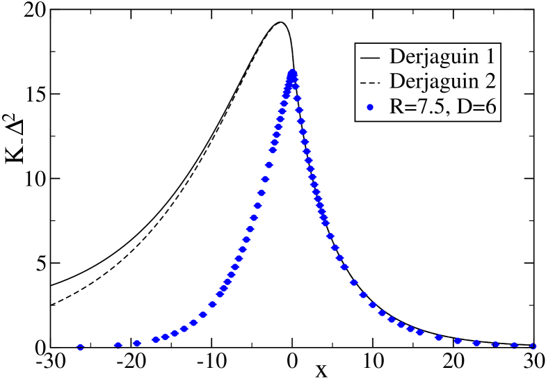
Figure 12: We plot $K_{-}(x,\Delta)\Delta^{2}$ as a function of $x$ for $\Delta\rightarrow 0$ obtained by using the Derjaguin approximation and $\Delta\approx 1$ using our Monte Carlo data for $R=7.5$ and $D=6$. Note that the index of $K$ indicates $s_{sphere}=-1$. In the case of the Derjaguin approximation we have used two different extrapolations of the scaling function $\theta_{+-}(x)$ for $x\lessapprox-48$ as discussed in the text.

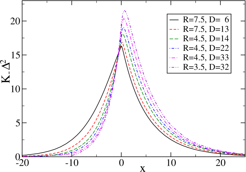
Figure 13: We plot $K_{-}(x,\Delta)\Delta^{2}$ as a function of $x$ for various values of $\Delta$. Note that the index of $K$ indicates $s_{sphere}=-1$. We use Monte Carlo data for $(R,D)$ = $(7.5,6)$, $(7.5,13)$, $(4.5,14)$, $(4.5,22)$, $(4.5,33)$, and $(3.5,32)$, corresponding to $\Delta\approx$ $1.03$, $2.06$, $4.02$, $6.13$, $9.04$, and $12.17$, respectively.

This observation might be explained as follows: Deep in the low temperature phase the physics of a film with $+-$ boundary conditions is governed by the interface between the two phases of positive and negative magnetisation. In the case of the film, this interface can move quite freely between the two plates. In contrast, in the case of the sphere-plate geometry, the interface is closely attached to the sphere, minimizing the area of the interface.

As for $s_{sphere}=1$ our observations for $s_{sphere}=-1$ are consistent with those of ref. troendle . For technical reasons the authors of troendle performed the mean-field calculation only for $\theta\geq 0$. This means that mean-field results for the low temperature phase, where we see a large deviation between the Derjaguin approximation and our Monte Carlo result for $\Delta\approx 1$ are unfortunately missing in Fig. 2 a of troendle .

In figure 13 we plot $K_{-}(x,\Delta)\Delta^{2}$ as a function of $x$ for various values of $\Delta$. With increasing $\Delta$ the maximum of $K_{-}(x,\Delta)\Delta^{2}$ increases and also $x_{max}$ slowly increases. For the range of $\Delta$ studied here, $K_{-}(x,\Delta)\Delta^{2}$ is increasing with increasing $\Delta$ for $x\gtrapprox-0.6$, while it is decreasing with increasing $\Delta$ for $x\lessapprox-0.6$.

Next we study in more detail the maximum of $K_{-}(x,\Delta)$ as a function of $x$. In figure 14 we plot the location $x_{max}$ of the maximum as a function of $\Delta$. Since $x_{max}$ is very close to zero, finite $L_{0}$ and $L$ effects might be large. In order to check for these effects, we plot for $R=4.5$ the results obtained by using lattices of the sizes $298\times 100^{2}$, $448\times 150^{2}$ and $598\times 200^{2}$. In fact for $\Delta\gtrapprox 3$ we see that the results obtained for the $298\times 100^{2}$ lattice clearly deviate from those for the other two lattice sizes. On the other hand, the results for the lattice sizes $448\times 150^{2}$ and $598\times 200^{2}$ are essentially consistent and are more or less consistent with those for $R=3.5$. Therefore we consider the results that we have obtained for our largest lattice sizes as reasonable approximation of the $L_{0},L\rightarrow\infty$ limit.

Using the Derjaguin approximation, we get $x_{max}\approx-1.43$ in the limit $\Delta\rightarrow 0$. Within the Derjaguin approximation $x_{max}$ is decreasing with increasing $\Delta$. In contrast for all values of $\Delta$ that we studied by Monte Carlo simulations, we find $x_{max}>0$. Looking at our data obtained for $R=7.5$ we estimate $x_{max}=0$ at $\Delta\approx 0.5$. $x_{max}$ slowly increases with increasing $\Delta$. For $\Delta\approx 12$ we get $x_{max}\approx 0.6$.

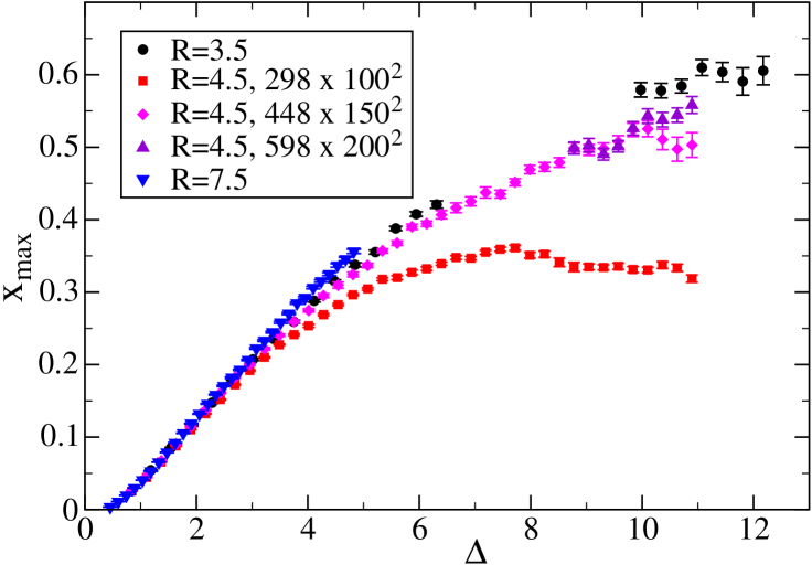
Figure 14: We plot $x_{max}$ as a function of $\Delta$ for $s_{sphere}=-1$. We give our results for $R=3.5$, $4.5$ and $7.5$. In the case of $R=4.5$ we compare the results obtained for the three different lattice sizes $298\times 100^{2}$, $448\times 150^{2}$, and $598\times 200^{2}$.

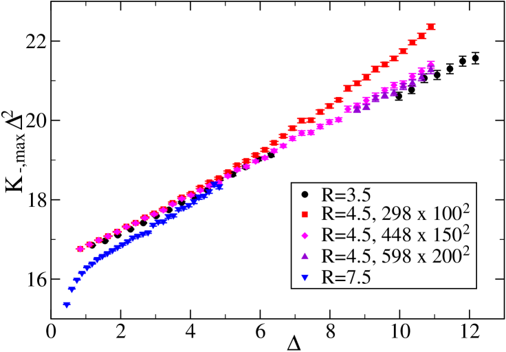
Figure 15: We plot $K_{-}(x_{max},\Delta)\Delta^{2}$ as a function of $\Delta$ for $s_{sphere}=-1$. We give our results for $R=3.5$, $4.5$ and $7.5$. In the case of $R=4.5$ we compare the results obtained for the three different lattice sizes $298\times 100^{2}$, $448\times 150^{2}$, and $598\times 200^{2}$.

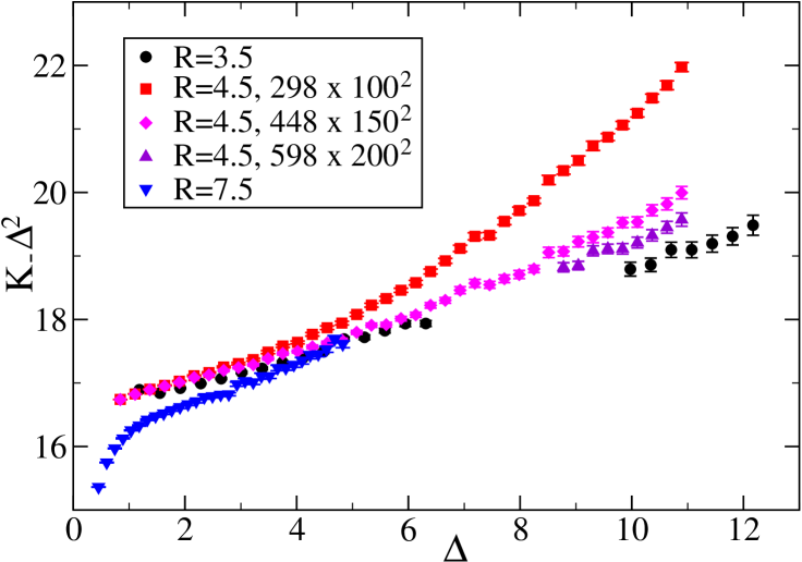
Figure 16: We plot $K_{-}(0,\Delta)\Delta^{2}$ as a function of $\Delta$ for $s_{sphere}=-1$. We give our results for $R=3.5$, $4.5$ and $7.5$. In the case of $R=4.5$ we compare the results obtained for the three different lattice sizes $298\times 100^{2}$, $448\times 150^{2}$, and $598\times 200^{2}$.

In figure 15 we plot $K_{-}(x_{max},\Delta)\Delta^{2}$ as a function of $\Delta$. Also here we check for finite $L_{0}$ and $L$ effects by plotting for $R=4.5$ the results obtained for three different lattice sizes. Also here we find that the result for the $298\times 100^{2}$ lattice differs from those for the $448\times 150^{2}$ and $598\times 200^{2}$ lattices for larger values of $\Delta$, while the results obtained for lattices of the sizes $448\times 150^{2}$ and $598\times 200^{2}$ are in quite good agreement. For $\Delta\lessapprox 4$ the results for $R=7.5$ and the other radii do not agree within error bars indicating violations of scaling that are larger than the numerical errors. Taking into account these observations we conclude that $K_{-}(x_{max},\Delta)\Delta^{2}$ increases roughly linearly in the range of $\Delta$ that we studied. We get $K_{-}(x_{max},\Delta)\Delta^{2}\approx 16$ for $\Delta\approx 1$ and $K_{-}(x_{max},\Delta)\Delta^{2}\approx 21.5$ for $\Delta\approx 12$. In the limit $\Delta\rightarrow 0$ we get $K_{-}(x_{max},\Delta)\Delta^{2}\approx 19.2$. Within the Derjaguin approximation $K_{-}(x_{max},\Delta)\Delta^{2}$ is decreasing with increasing $\Delta$. Hence $K_{-}(x_{max},\Delta)\Delta^{2}$ should reach a minimum in the interval $0<\Delta\lessapprox 1$.

In figure 16 we plot $K_{-}(0,\Delta)\Delta^{2}$ as a function of $\Delta$. Our observations concerning finite $L_{0}$ and $L$ effects and scaling are qualitatively similar as for $K_{-}(x_{max},\Delta)\Delta^{2}$. However the amplitudes of the differences are larger than for $K_{-}(x_{max},\Delta)\Delta^{2}$. For large values of $\Delta$ even the results for the lattice sizes $448\times 150^{2}$ and $598\times 200^{2}$ do not agree within the statistical error. Taking into account these observation we conclude that $K_{-}(0,\Delta)\Delta^{2}$ is increasing roughly linearly in the range $1\lessapprox\Delta\lessapprox 12$. We get $K_{-}(x_{max},\Delta)\Delta^{2}\approx 16$ for $\Delta\approx 1$ and $K_{-}(x_{max},\Delta)\Delta^{2}\approx 19.5$ for $\Delta\approx 12$. In the Derjaguin approximation we get $\lim_{\Delta\rightarrow 0}K_{-}(0,\Delta)\Delta^{2}\approx 17.6$. In the Derjaguin approximation, $K_{-}(0,\Delta)\Delta^{2}$ is decreasing with increasing $\Delta$. Therefore, as it is the case for $K_{-}(x_{max},\Delta)\Delta^{2}$, $K_{-}(0,\Delta)\Delta^{2}$ should show a minimum in the interval $0<\Delta\lessapprox 1$.

V.6 Small sphere expansion at the critical point

In the limit $D\gg R$ the behaviour of the reduced excess free energy at the critical point is given by BuEi97

$$F_{ex}(D,R)=-\frac{A_{a}^{\psi}A_{b}^{\psi}}{B_{\psi}}\left(\frac{R}{2D}\right)^{x_{\psi}}$$ (20)

where $x_{\psi}$ is the dimension of the field $\psi$. The amplitudes are defined by

$$\langle\psi_{0}\psi_{r}\rangle_{bulk}=B_{\psi}r^{-2x_{\psi}}$$ (21)

and

$$\langle\psi_{r}\rangle_{halfspace}^{a}=A_{a}^{\psi}(2r)^{-x_{\psi}}$$ (22)

where in the case of eq. (22) $r$ is the distance from the boundary of type $a$. For the boundary conditions discussed here, the leading contribution comes from the order parameter $\phi$ with

$$x_{\phi}=\beta/\nu=\frac{1}{2}(d-2+\eta)$$ (23)

where $\eta=0.03627(10)$ mycritical . The subleading contribution is due to the energy density $\epsilon$ with

$$x_{\epsilon}=d-1/\nu$$ (24)

where $\nu=0.63002(10)$ mycritical .

In relation with ref. mycrossover we had simulated $512^{3}$ lattices with $++$ and $+0$ boundary conditions in one direction and periodic ones in the other two directions at $\beta=0.387721735$. We had measured the magnetisation profile. Taking into account the extrapolation length, we get from the magnetisation profile at $r\approx 30$ the estimate

$$A_{+}^{\phi}=1.1268(5)\;\;.$$ (25)

In order to compute the amplitude $B_{\phi}$ we simulated systems with periodic boundary conditions in all three directions. We simulated lattices of the sizes $128^{3}$, $256^{3}$, $512^{3}$ and $1024^{3}$ at $\beta=0.387721735$. We measured $\langle s_{x}s_{y}\rangle$ for $y-x=(i,0,0)$, $(0,i,0)$ and $(0,0,i)$ and $i=1,2,...$ . Using the numerical results of the two-point function we computed

$$B_{\phi,eff}(i)=i^{2x_{\phi}}\langle s_{x}s_{x+(i,0,0)}\rangle$$ (26)

using $2x_{\phi}=1.03627(10)$. It turns out that $B_{\phi,eff}(i)$ shows a shallow minimum for a rather small value of $i$. At larger distances, $B_{\phi,eff}(i)$ increases due to the periodic boundary conditions imposed. The minimum is given by $(i_{min},B_{\phi,eff,min})=$ $(4,0.19397(8))$, $(6,0.19026(15))$, $(7,0.18838(11))$, and $(8,0.18745(13))$ for lattices of the size $128^{3}$, $256^{3}$, $512^{3}$ and $1024^{3}$, respectively. Assuming power like corrections, we arrive at our final estimate

$$B_{\phi}=0.1865(3)\;\;.$$ (27)

Combining eqs. (25,27) we arrive at

$$a=\frac{A_{+}^{\psi}A_{+}^{\psi}}{B_{\psi}}=6.808(12)\;\;.$$ (28)

This result can be compared with $a\approx 7.73$ given in ref. HaScEiDi98 , where the authors had deduced the estimate for three dimensions from the exact result in two dimensions and the $\epsilon$-expansion. For a discussion see footnote [13] of ref. HaScEiDi98 .

As check we computed $Z_{-}/Z_{+}$ for the radii $R=3.5$ using the sphere flip algorithm discussed in Appendix B. We have simulated lattices of the size $L_{0}\times L^{2}$ where we have fixed $s_{x}=1$ for $x_{0}=0$ and $s_{x}=0$ for $x_{0}=L_{0}+1$. Our numerical results for $R=3.5$ are summarized in table 2. First we have simulated for $h=D+R=72$ lattices of different linear sizes $L_{0}$ and $L$ in order to check numerically the effect of the finite size of the lattice. We expect that at the critical point, the result for $Z_{-}/Z_{+}$ converges with a power law to the $L_{0},L\rightarrow\infty$ limit. The results of $(L_{0},L)=(499,400)$ and $(L_{0},L)=(799,600)$ are consistent within the statistical error. Next we simulated lattices of the size $(L_{0},L)=(499,400)$ for various values of $h=D+R$.

Inserting $A_{+}^{\psi}=-A_{-}^{\psi}$ into eq. (20) we get for $D\gg R$

$$-\ln(Z_{-}/Z_{+})=2\frac{A_{+}^{\psi}A_{+}^{\psi}}{B_{\psi}}\left(\frac{R}{2D}\right)^{x_{\psi}}\;\;.$$ (29)

For finite $D$ we define

$$a(D)=-\frac{1}{\ln(Z_{-}/Z_{+})}\left(\frac{2D_{eff}}{R_{eff}}\right)^{x_{\psi}}\;\;,$$ (30)

where we replaced $R$ and $D$ by $R_{eff}$, table 5, and $D_{eff}$, eq. (9), respectively, to reduce corrections to scaling.

Table 2: Results for the ratio $Z_{-}/Z_{+}$ of partition functions for the radius $R=3.5$. In the fourth column we give the number of measurements. In the last column we give the estimate of the universal ratio $a$. In $()$ we give the error due to the statistical error of $Z_{-}/Z_{+}$ and in $[]$ the error due to the uncertainty of $R_{eff}$. For a discussion see the text.

$h=D+R$	$L_{0}$	$L$	stat	$Z_{-}/Z_{+}$	aaa $a$
72	199	160	$10^{5}$	0.1645(28)
72	299	250	$10^{5}$	0.1472(26)
72	359	300	$10^{5}$	0.1449(26)
72	499	400	$1.5\times 10^{5}$	0.1391(21)	7.57(6)[9]
72	799	600	$10^{5}$	0.1384(25)
30	499	400	$1.2\times 10^{5}$	0.0289(7)	8.43(6)[11]
40	499	400	$1.2\times 10^{5}$	0.0552(12)	8.09(6)[10]
50	499	400	$1.2\times 10^{5}$	0.0761(15)	8.12(6)[10]
60	499	400	$10^{5}$	0.1090(20)	7.71(6)[9]
90	499	400	$1.2\times 10^{5}$	0.1830(27)	7.34(6)[9]

In the last column of table 2 we give estimates of $a$ obtained for various distances $D$. It is decreasing with increasing distances. For the largest distance that we simulated, it is still clearly larger than the estimate (28), indicating that still at $\Delta\approx 30$ subleading contributions to $F_{ex}$ are significant.

VI Conclusions and outlook

We have demonstrated how the thermodynamic Casimir force for the sphere-plate geometry can be computed efficiently by Monte Carlo simulations of spin models. Similar to the proposal of Hucht Hucht for the plate-plate geometry, we compute differences of the free energy by integrating differences of the energy over the inverse temperature. For $R\ll L_{0},L$, where $R$ is the radius of the sphere and $L_{0},L$ are the linear extensions of the lattice, such energy differences, when determined the standard way, are affected by a huge relative variance. Here we demonstrate how this problem can be overcome by using the exchange cluster algorithm HeBl98 . Using the exchange cluster algorithm we define an improved estimator for the energy differences with a strongly reduced variance. For a detailed discussion see section IV. We simulated the improved Blume-Capel model, which shares the universality class of the three-dimensional Ising model. Improved means that the amplitudes of the leading bulk correction are strongly suppressed. We studied strongly symmetry breaking boundary conditions. We fixed the spins at the boundary to $s_{x}=1$. The spins at the surface of the sphere are fixed to $s_{x}=s_{sphere}$, where we studied the two cases $s_{sphere}=-1$ and $1$ in detail. First we verified that the method is efficient for a large range of parameters. We studied the whole range of temperatures where the thermodynamic Casimir force has a significant amplitude. We considered distances between the sphere and the plate up to $D_{max}=32$, $40$, $32$ and $10$ for the radii $R=3.5$, $4.5$, $7.5$ and $15.5$, respectively. In order to see a good scaling behaviour of the data obtained for different radii, we introduced an effective radius $R_{eff}$ of the spheres that we determined by using a particular finite size scaling analysis. For details see Appendix A. We obtain reliable results for the scaling functions $K_{+}(x,\Delta)$ and $K_{-}(x,\Delta)$ for the whole range of $x$ and $1\lessapprox\Delta\lessapprox 12$, where $x=t[D/\xi_{0}]^{1/\nu}$ and $\Delta=D/R$. Smaller values of $\Delta$ would be desirable to make better contact with the Derjaguin approximation and larger ones to reach the range of validity of the small sphere expansion. For $s_{sphere}=1$ we find that for the values of $\Delta$ studied here, the shape of $K_{+}(x,\Delta)\Delta^{2}$ viewed as a function of $x$ is quite similar to that of $\lim_{\Delta\rightarrow 0}K_{+}(x,\Delta)\Delta^{2}$ obtained by using the Derjaguin approximation. For $s_{sphere}=-1$ in the high temperature phase still the same observation holds, however in the low temperature phase $K_{-}(x,\Delta)\Delta^{2}$ is strongly suppressed for $\Delta\gtrapprox 1$ compared with $\Delta\rightarrow 0$. We attribute this behaviour to the fact that the interface between positive and negative magnetisation is closely attached to the sphere, in order to minimize the area of the interface. In contrast, for the film geometry, the interface is moving quite freely between the boundaries. Finally, by using a different cluster algorithm, which is similar to the boundary flip algorithm MH93A ; MH93B , we computed the difference of reduced free energies $F_{-}-F_{+}$ for large distances $D$ at the critical point, where the subscript of $F$ gives the sign of $s_{sphere}$. Here we made contact with the small sphere expansion. Still for $\Delta\approx 30$ we see a deviation from the leading order of the small sphere expansion at the level of about $7\%$.

The present work should be seen as a pilot study. It can be improved and extended in many respects. Our preliminary study for $s_{sphere}=0$ discussed in section V.2 indicates that for $s_{sphere}=0$ the performance of the exchange cluster algorithm is worse than for $s_{sphere}=\pm 1$, however still it seems likely that physically relevant results can be obtained. Based on this experience we are confident that the algorithm discussed here can be applied to a variety of experimentally relevant situations. E.g. the crossover of boundary universality classes or patterned surfaces. In particular also the sphere-sphere geometry should be accessible by the algorithm discussed here. One might also check whether the exchange cluster algorithm allows to improve the results for the film geometry that have been obtained so far using standard simulation algorithms.

One could improve the present study by various means. In order to reach larger lattice sizes one might implement the computer program by using the multispin-coding technique. To this end one might also try to simulate with a varying lattice resolution: spins far away from the sphere could be replaced by block-spins. In order to reduce corrections to scaling one might try to improve the spherical shape of the sphere by tuning the couplings at the surface of the sphere.

VII Acknowledgement

This work was supported by the DFG under the grant No HA 3150/2-2.

Appendix A Determination of the effective radius $R_{eff}$

In order to determine the effective radius of the sphere, we studied the ratio of partition functions $r=Z_{-}/Z_{+}$ for a lattice of the linear sizes $L_{0}$ and $L_{1}=L_{2}=L$, where the sphere is placed exactly in the middle of the system; i.e. $h=(L_{0}+1)/2$ for odd values of $L_{0}$. The spins at $x_{0}=0$ and $x_{0}=L_{0}+1$ are fixed to $s_{x}=1$. The index of $Z$ refers to the sign of $s_{sphere}$. At the critical point, in the scaling limit

$$r(R,L_{0},L)=G(R/L_{0},L/L_{0})\;\;.$$ (31)

In the following, we restrict ourselves to $L/L_{0}=1/2$ and define $g(R/L_{0})=G(R/L_{0},1/2)$. Furthermore we require that the ratio of partition functions assumes a fixed value. Our ad hoc choice is $r=0.1$. For a given radius $R$ this fixes the linear size of the lattice to $L_{0}=L_{0,fix}$. In order to reduce corrections to scaling we replace $L_{0}$ by $L_{0,eff}=L_{0}+L_{s}$ using $L_{s}=1.92$ mycrossover . Since $L$ assumes integer and $L_{0}$ odd integer values, we interpolate or extrapolate $r(R,L_{0},L)$ to $r(R,L_{0},L_{0,eff}/2)$. To this end, we simulated for $R=3.5$ and $L_{0}=131$ the linear extensions $L=64$, $66$ and $68$. The results are $r=0.10405(23)$, $0.10015(16)$ and $0.09641(22)$, respectively. We performed $10^{7}$, $2\times 10^{7}$ and $10^{7}$ measurements for $L=64$, $66$ and $68$, respectively. In order to apply the result also to other radii, we compute

$$\left.\frac{\partial r}{\partial(L/L_{0,eff})}\right|_{L/L_{0,eff}=0.5,L_{0}=L_{0,fix}}=-0.254(11)$$ (32)

where we have used the finite difference of the estimates for $L=64$ and $68$. For larger radii we have simulated $L=(L_{0}+1)/2$ and have extrapolated $r$ to $L=(L_{0}+1.92)/2$ by using eq. (32). In addition to $R=3.5$ we have simulated the radii $R=4.5$, $5.5$, $6.5$, $7.5$, $9.5$, $12.5$ and $15.5$. We performed $8\times 10^{6}$ measurements for $R=4.5$ down to $3.4\times 10^{6}$ measurements for $R=15.5$. In total these simulations took about 5 years of CPU-time on a single core of a Quad-Core AMD Opteron(tm) 2378 CPU running at 2.4 GHz. Our results for $L_{0}$ such that $r\approx 0.1$ are summarized in table 3. We linearly extrapolate $r(R,L_{0},L_{0,eff}/2)$ in $L_{0}$. To this end, we use

$$L_{0,eff}\frac{\partial r(R,L_{0},L_{0,eff}/2)}{\partial L_{0}}=0.11(1)$$ (33)

which we have computed by using finite differences. Solving $r(R,L_{0},L_{0,eff}/2)=0.1$ with respect to $L_{0}$ we arrive at the estimate of $L_{0,eff,fix}$ given in the last column of table 3.

Table 3: Estimates of $r(R,L_{0},L_{0,eff}/2)$ for $L_{0}$ such that $r\approx 0.1$. In the last column we give the solution of $r(R,L_{0},L_{0,eff}/2)=0.1$. For a discussion see the text.

$R$	$L_{0}$	$r$	$L_{0,eff,fix}$
3.5	131	0.09927(20)	133.8(3)
4.5	183	0.09972(30)	185.4(6)
5.5	235	0.09922(32)	238.6(0.8)
6.5	287	0.10162(32)	284.7(1.3)
7.5	331	0.09903(39)	335.9(1.5)
9.5	435	0.10027(41)	435.8(1.7)
11.5	535	0.10103(43)	531.9(2.6)
15.5	731	0.10065(57)	728.6(4.2)

Now we define the effective radius by

$$R_{eff}=c^{-1}L_{0,eff,fix}(R)$$ (34)

In order to determine the factor $c$ we fitted our data with the Ansatz

$$L_{0,eff,fix}(R)=c[R+R_{s}]\;\;.$$ (35)

where $c$ and $R_{s}$ are the parameters of the fit and with

$$L_{0,eff,fix}(R)=c[R+R_{s}]\times(1+b[R+R_{s}]^{-2})$$ (36)

with the additional free parameter $b$. The results of our fits are summarized in table 4. As our final estimate we take $c=49(1)$ which is consistent with all results given in table 4.

Table 4: Results of fits with the Ansätze (35,36). All data with $R_{min}\leq R\leq 15.5$ are taken into account. In the case of the Ansatz (36) we do not report the estimates of $b$.

Ansatz	$R_{min}$	$c$	$R_{s}$	$\chi^{2}/$d.o.f.
35	4.5	49.65(22)	–0.74(2)	3.11
35	5.5	49.08(28)	–0.65(4)	1.19
35	6.5	49.47(37)	–0.72(6)	0.78
36	3.5	49.00(31)	–0.61(5)	1.97
36	4.5	48.57(41)	–0.52(8)	2.07

Finally in table 5 we summarize the results for the effective radii $R_{eff}$ for the values of $R$ that are studied in the remainder of the paper.

Table 5: Results for the effective radius $R_{eff}$ obtained by using eq. (34) and the estimate $c=49(1)$.

$R$	$R_{eff}$
3.5	2.73(6)
4.5	3.78(9)
7.5	6.86(17)
15.5	14.87(38)

Appendix B The sphere flip algorithm

In Appendix A and section V.6 we have computed the ratio

$$r=\frac{Z_{-}}{Z_{+}}$$ (37)

by using a special cluster algorithm. The index of the partition function $Z$ refers to the sign $s_{sphere}$ of the sphere. This cluster algorithm is closely related to the boundary flip algorithm discussed in refs. MH93A ; MH93B that allows to compute the ratio $Z_{a}/Z_{p}$, where $p$ refers to periodic and $a$ to anti-periodic boundary conditions. In ref. mycorrection we had employed a similar algorithm to compute $Z_{-+}/Z_{++}$, where the indices of $Z$ refer to the signs of the spins at the boundaries.

Let us consider the composed system

$$Z=Z_{-}+Z_{+}=\sum_{s_{sphere}=\pm 1}\sum_{\{s\}}\exp(-H(\{s\},s_{sphere}))$$ (38)

where $s_{sphere}$ can be viewed as an Ising spin. This system can be updated by using the standard cluster algorithm. When the cluster that contains the sphere is not frozen to the boundary, $s_{sphere}$ can be flipped. In this composed system, the ratio $r=Z_{-}/Z_{+}$ is given by the ratio of expectation values $r=\langle\delta_{-1,s_{sphere}}\rangle/\langle\delta_{1,s_{sphere}}\rangle$.

In fact it is sufficient to simulate $Z_{+}$ only. Since for $s_{sphere}=-1$ the cluster that contains the sphere never freezes to the boundary it is sufficient to compute the fraction of cluster updates that would allow to update $s_{sphere}=1$ to $s_{sphere}=-1$. To this end, on has to check for each cluster update, whether the cluster that contains the sphere is frozen to the boundary. In the composed system

$$\frac{Z_{-}}{Z_{+}}=\frac{p(+\rightarrow-)}{p(-\rightarrow+)}=p(+\rightarrow-)$$ (39)

where $p(-\rightarrow+)$ and $p(-\rightarrow+)$ are the probabilities to update $s_{sphere}=-1$ to $s_{sphere}=1$ and vice versa, respectively. As discussed above $p(-\rightarrow+)=1$.

We have updated the $s_{sphere}=1$ system by a combination of the local heat-bath algorithm and the Swendsen-Wang cluster algorithm SwWa87 . In the case of the Swendsen-Wang cluster algorithm SwWa87 the boundary conditions have to be taken into account: All spins that belong to clusters that are frozen to the boundary or contain the sphere keep their value. All other clusters are flipped with the probability $1/2$, where flipped means that the sign of all spins in a given cluster is changed.

References

- (1) M. E. Fisher and P.-G. de Gennes, CR Seances Acad. Sci. Ser. B 287, 207 (1978)
- (2) A. Gambassi, [arXiv:0812.0935], J. Phys. Conf. Ser. 161, 012037 (2009)
- (3) Roger H. French et al. Rev. Mod. Phys 82 1887, (2010)
- (4) R. Garcia and M. H. W. Chan, Phys. Rev. Lett. 83 1187, (1999)
- (5) R. Garcia and M. H. W. Chan, Phys. Rev. Lett. 88, 086101 (2002)
- (6) A. Ganshin, S. Scheidemantel, R. Garcia, and M. H. W. Chan, Phys. Rev. Lett. 97 075301, (2006)
- (7) Masafumi Fukuto, Yohko F. Yano, and Peter S. Pershan Phys. Rev. Lett. 94, 135702 (2005)
- (8) Salima Rafaï, Daniel Bonn, Jacques Meunier, Physica A 386, 31 (2007)
- (9) M. Krech, The Casimir Effect in Critical Systems (World Scientific, Singapore, 1994)
- (10) H. W. Diehl, Field-theoretical Approach to Critical Behaviour at Surfaces in Phase Transitions and Critical Phenomena, edited by C. Domb and J.L. Lebowitz, Vol. 10 (Academic, London 1986) p. 76
- (11) H. W. Diehl, [cond-mat/9610143], Int. J. Mod. Phys. B 11, 3503 (1997)
- (12) A. Hucht, [arXiv:0706.3458], Phys. Rev. Lett. 99, 185301 (2007)
- (13) O. Vasilyev, A. Gambassi, A. Maciołek, and S. Dietrich, [arXiv:0812.0750], Phys. Rev. E 79 041142, (2009)
- (14) M. Hasenbusch, [arXiv:0905.2096], J. Stat. Mech. (2009) P07031
- (15) M. Hasenbusch, [arXiv:0907.2847], Phys. Rev. B 81, 165412 (2010)
- (16) D. Dantchev and M. Krech, Phys. Rev. E 69, 046119 (2004)
- (17) O. Vasilyev, A. Gambassi, A. Maciołek, and S. Dietrich, [arXiv:0708.2902], Europhys. Lett. 80, 60009 (2007)
- (18) M. Hasenbusch, [arXiv:1005.4749], Phys. Rev. B 82, 104425 (2010)
- (19) Francesco Parisen Toldin, Siegfried Dietrich, [arXiv:1007.3913] J. Stat. Mech. (2010) P11003
- (20) M. Hasenbusch, [arXiv:1012.4986], Phys. Rev. B 83, 134425 (2011)
- (21) O. Vasilyev, A. Maciołek, and S. Dietrich, [arXiv:1106.5140], Phys. Rev. E 84, 041605 (2011)
- (22) Alfred Hucht, Daniel Grüneberg, Felix M. Schmidt, [arXiv:1012.4399], Phys. Rev. E 83, 051101 (2011)
- (23) M. Hasenbusch, [arXiv:1202.6206], Phys. Rev. B 85, 174421 (2012)
- (24) C. Hertlein, L. Helden, A. Gambassi, S. Dietrich, and C. Bechinger, Nature 451, 172 (2008)
- (25) A. Gambassi, A. Maciołek, C. Hertlein, U. Nellen, L. Helden, C. Bechinger, and S. Dietrich, [arXiv:0908.1795], Phys. Rev. E 80, 061143 (2009)
- (26) U. Nellen, L. Helden and C. Bechinger, EPL 88, 26001 (2009)
- (27) F. Soyka, O. Zvyagolskaya, Ch. Hertlein, L. Helden, and C. Bechinger, Phys. Rev. Lett. 101, 208301 (2008)
- (28) M. Tröndle, O. Zvyagolskaya, A. Gambassi, D. Vogt, L. Harnau, C. Bechinger, and S. Dietrich, Molecular Physics 109, 1169 (2011)
- (29) O. V. Zvyagolskaya, Kritischer Casimir-Effekt in kolloidalen Modellsystemen, PhD thesis, Physikalisches Institut der Universität Stuttgart, elib.uni-stuttgart.de/opus/volltexte/2012/7347/index.html
- (30) Daniel Bonn, Jakub Otwinowski, Stefano Sacanna, Hua Guo, Gerard Wegdam, and Peter Schall, Phys. Rev. Lett. 103, 156101 (2009); Andrea Gambassi and S. Dietrich Phys. Rev. Lett. 105, 059601 (2010); Bonn, Wegdam, and Schall Reply: Daniel Bonn, Gerard Wegdam, and Peter Schall Phys. Rev. Lett. 105, 059602 (2010)
- (31) O. Zvyagolskaya, A. J. Archer and C. Bechinger, EPL 96, 28005 (2011)
- (32) A. Hanke, F. Schlesener, E. Eisenriegler, and S. Dietrich, Phys. Rev. Lett. 81, 1885 (1998)
- (33) B. V. Derjaguin, Kolloid Z. 69, 155 (1934)
- (34) T. W. Burkhardt and E. Eisenriegler, Phys. Rev. Lett. 74, 3189 (1995); 78, 2867 (1997); E. Eisenriegler and U. Ritschel, Phys. Rev. B 51, 13717 (1995)
- (35) M. Tröndle, S. Kondrat, A. Gambassi, L. Harnau, and S. Dietrich, [arXiv:1005.1182], J. Chem. Phys. 133, 074702 (2010)
- (36) J.R. Heringa and H. W. J. Blöte, Phys. Rev. E 57, 4976 (1998)
- (37) M. Hasenbusch, [hep-lat/9209016], J. Phys. I (France) 3, 753 (1993)
- (38) M. Hasenbusch, Physica A 197, 423 (1993)
- (39) Y. Deng and H. W. J. Blöte, Phys. Rev. E 70, 046111 (2004)
- (40) M. Hasenbusch, [arXiv:1004.4486], Phys. Rev. B 82, 174433 (2010)
- (41) M. Campostrini, A. Pelissetto, P. Rossi and E. Vicari, [cond-mat/0201180], Phys. Rev. E 65, 066127 (2002)
- (42) Robert H. Swendsen and Jian-Sheng Wang, Phys. Rev. Lett. 57, 2607 (1986)
- (43) Robert H. Swendsen and Jian-Sheng Wang, Phys. Rev. Lett. 58, 86 (1987)
- (44) U. Wolff, Phys. Rev. Lett. 62, 361 (1989)
- (45) M. Hasenbusch, K. Pinn and S. Vinti, Phys. Rev. B 59, 11471 (1999).
- (46) W. Kerler, Phys. Rev. D 47 1285, (1993)
- (47) M. Saito and M. Matsumoto, “SIMD-oriented Fast Mersenne Twister: a 128-bit Pseudorandom Number Generator”, in Monte Carlo and Quasi-Monte Carlo Methods 2006, edited by A. Keller, S. Heinrich, H. Niederreiter, (Springer, 2008); M. Saito, Masters thesis, Math. Dept., Graduate School of science, Hiroshima University, 2007. The source code of the program is provided at “http://www.math.sci.hiroshima-u.ac.jp/m-mat/MT/SFMT/index.html”