Statistical fluctuation analysis for measurement-device-independent quantum key distribution

Abstract

Measurement-device-independent quantum key distribution with a finite number of decoy states is analyzed under finite-data-size assumption. By accounting for statistical fluctuations in parameter estimation, we investigate vacuum+weak- and vacuum+two-weak-decoy-state protocols. In each case, we find proper operation regimes, where the performance of our system is comparable to the asymptotic case for which the key size and the number of decoy states approach infinity. Our results show that practical implementations of this scheme can be both secure and efficient.

I Introduction

Quantum key distribution (QKD) Bennett and Brassard (1984); Ekert (1991) is one of the most successful applications of quantum information processing, which allows two distant parties, Alice and Bob, to grow secret keys with information-theoretic security Mayers (2001); Lo and Chau (1999); Shor and Preskill (2000); Biham et al. (2000); Inamori et al. (2007); Renner et al. (2005). Conventional security proofs of QKD assume certain physical models for the employed devices — source and detection units. For instance, the squashing model is widely assumed for the measurement Beaudry et al. (2008); Tsurumaru and Tamaki (2008); Fung et al. (2011) in a standard security analysis Gottesman et al. (2004). Practical implementations, however, could fall short of meeting all requirements set by the models, hence security could be compromised in reality. In fact, side channels have been identified and exploited to break QKD security. These side-channel attacks include the fake-state attack Makarov et al. (2006); Makarov and Skaar (2008), the time-shift attack Qi et al. (2007); Zhao et al. (2008), the phase-remapping attack Fung et al. (2007); Xu et al. , and the detector-blinding attack Lydersen et al. (2010); Gerhardt et al. (2011).

Several approaches have been proposed to counter the side-channel attacks. One way is to sufficiently characterize the behavior of the devices and analyze the security by taking into account all device parameters Fung et al. (2009); Lydersen and Skaar (2010); Marøy et al. (2010). This, however, can be difficult to implement in practice. A second approach that can defeat all side-channel attacks is device-independent QKD Mayers and Yao (1998); Acín et al. (2007); Pironio et al. (2009), in which the security can be proven without knowing the specifications of the devices used. Security, in this case, is derived from nonlocal correlations by violating Bell’s inequality Bell (1964); Clauser et al. (1969). In order to avoid the detection efficiency loophole Pearle (1970), however, a large fraction of the transmitted signals must be detected by the receiver, resulting in impractical requirements for the transmission efficiency (e.g., $82.8\%$ Garg and Mermin (1987) for the Clauser-Horne-Shimony-Holt (CHSH) inequality Clauser et al. (1969)).

Instead of full device independence, a detection-device independent QKD scheme is proposed Ma and Lütkenhaus (2012); Pawłowski and Brunner (2011), in which the detection system is assumed to be untrusted. Since most of practical hacking strategies focus on the detection site, and the source site is relatively simple for characterization, such a scheme can close most loopholes in a QKD system. Unfortunately, these schemes still need stringent requirements on the transmission efficiency of more than 50% Ma and Lütkenhaus (2012).

Recently, Lo, Curty, and Qi Lo et al. (2012) proposed efficient schemes that are measurement-device independent (MDI). Alice and Bob send some signals to a willing participant who can even be an eavesdropper, Eve. Eve performs a Bell-state measurement (BSM) and announces the result to Alice and Bob who will use this information to distill a secret key. The security is based on the idea of entanglement swapping using a BSM and the reverse EPR QKD scheme Biham et al. (1996); Inamori (2002); Braunstein and Pirandola (2012). The scheme is secure even if Eve intentionally makes the wrong measurement and/or announces the wrong information. Various implementation approaches to MDI-QKD have also been proposed Tamaki et al. (2012); Ma and Razavi (2012), and significant efforts have been devoted to its experimental demonstration Lo et al. (2012); Rubenok et al. (2012); da Silva et al. (2012). Recently, the first MDI-QKD experiment with decoy states is completed by Liu et al. Liu et al. (2012).

MDI-QKD is not completely device independent and the source devices have to be trusted and sufficiently characterized. When we use a coherent source to implement a single-photon-based MDI-QKD scheme, such as that in Ref. Lo et al. (2012), we need to estimate the single-photon contributions of the detection at the receiver, which can be done efficiently using decoy states Hwang (2003); Lo et al. (2005); Ma et al. (2005); Wang (2005); *Wang:Decoy2:2005. In Lo et al. (2012), a security analysis is provided for the decoy-state MDI-QKD assuming infinitely long keys with infinitely many decoy states. In this paper, we proceed further and analyze the performance of decoy-state MDI-QKD when only a finite number of decoy states are used. Moreover, we consider statistical fluctuations caused by a finite-size key. Such an analysis is crucial to ensure the security of MDI-QKD in practical setups.

We note that the effect of finite size on MDI-QKD has also been recently studied in an independent work by Song et al. Song et al. (2012). However, they only analyzed the vacuum+weak-decoy-state protocol whereas we also analyze the vacuum+two-weak-decoy-state protocol here taking advantage of our general method which can easily be adapted to other decoy-state protocols.

The rest of this paper is organized as follows. In Sec. II, we briefly review the MDI-QKD scheme with decoy states. In Sec. III, we investigate the QKD model for the security proof and simulation. In Sec. IV, we perform a statistical fluctuation analysis on MDI-QKD systems, followed by numerical results in Sec. V. We conclude the paper in Sec. VI with remarks.

II Decoy-state MDI-QKD

The most general encoding scheme for BB84-based QKD relies on using two optical orthogonal modes. Here, we encode a qubit in the $z$ basis by using two spatially separated modes, $r$ and $s$, as shown in Fig. 1. That is, for the $z$ basis, the information is encoded in whether the photon is in mode $r$ or $s$. The qubit can also be encoded into the relative phases between modes $r$ and $s$. Denote $x$ basis to be the case when two relative phases $\{0,\pi\}$ are used and $y$ basis for $\{\pi/2,3\pi/2\}$. This encoding is sufficiently general to be tailored down to all proposed MDI-QKD schemes. For example, in the original MDI-QKD Lo et al. (2012), $r$ and $s$ correspond to $H$ and $V$ polarizations. For BB84 encoding, the $z$ and $x$ basis is used Lo et al. (2012). We remark that this setup can be used to implement the six-state QKD protocol as well Bruß (1998). For practical purposes, one may consider using temporal, rather than the spatial, modes as proposed in Ma and Razavi (2012); Rubenok et al. (2012). Here, however, we are mostly concerned with statistical fluctuation effects due to the finite size of the key, and our results are independent of the employed setup. The key assumption in all MDI-QKD schemes is that the photons on which the intermediary BSM is performed are indistinguishable. We assume this condition is held throughout our analysis.

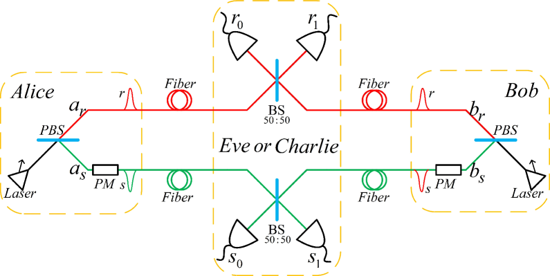
Figure 1: (Color Online) A schematic diagram for the MDI-QKD protocol, where PBS stands for polarizing beam splitter and PM stands for phase modulator. In order to encode their bits in the $z$ basis, Alice and Bob generate phase-randomized coherent states with either $H$ or $V$ polarizations at their sources. To encode a bit in the $x$ or $y$ basis, they generate $+45$-polarized signals at their encoders. A PM will introduce a relative phase shift between their reference and signal beams. The phase shifts are chosen from the set $\{0,\pi\}$ for the $x$ basis and $\{\pi/2,3\pi/2\}$ for the $y$ basis. A partial BSM, possibly performed by an untrusted party, Eve or Charlie, on the two reference and the two signal modes would establish correlations between the raw key bits of Alice and Bob. If they both use the $z$ basis, a click on exactly one of the $r$ detectors and exactly one of the $s$ detectors would imply anti-correlated bits shared between Alice and Bob. For $x$ and $y$ bases, if they both use the same basis, a joint click on detectors $r_{0}$ and $s_{0}$ implies identical bits for Alice and Bob; so does a joint click on $r_{1}$ and $s_{1}$. A joint click on $r_{0}$ and $s_{1}$, or, $r_{1}$ and $s_{0}$ would imply anticorrelated bits Ma and Razavi (2012).

In this paper, we assume that Alice and Bob use coherent states as their sources and use the $z$ and $x$ basis above for encoding. The MDI-QKD scheme runs as follows.

1. Alice randomly chooses a basis from $\{x,z\}$ and a bit from $\{0,1\}$, and sends a coherent-state pulse with intensity randomly chosen from a predetermined set. As shown in Fig. 1, if she picks the $z$ basis, she prepares her coherent states with either $H$ or $V$ polarizations depending on the bit value. Otherwise, if she picks the $x$ basis, she prepares $+45$-polarized signals, splits the pulse into two modes, $r$ and $s$, through a polarizing beam splitter (PBS), and encodes the bit values into relative phases, $\{0,\pi\}$, between the two modes. Bob applies the same encoding procedure.

2. Alice and Bob send the pulses to the relay, which can be fully controlled by Eve. Eve performs a partial BSM on the received pulses, as shown in Fig. 1. Eve announces her detection results. She is allowed to be dishonest.

3. Alice and Bob compare the bases used for all transmissions which include the no-detection events, successful BSM events, and unsuccessful BSM events.

4. Based on Eve’s announcement for each pulse, Alice and Bob keep the bit if it corresponds to a successful BSM event and a compatible basis has been used. One of them also flips the bit value in the case of an anticorrelated BSM result (see Fig. 1). They discard all other bits corresponding to the no-detection events, unsuccessful BSM events, and those with incompatible bases.

5. For each combination of Alice’s intensity $\mu$, Bob’s intensity $\nu$, and basis $w=x,z$, they test the error rate $E_{\mu\nu}^{w}$ of the retained bits, and compute the gain $Q_{\mu\nu}^{w}$ by counting the number of successful BSM events among all transmissions (including the no-detection events, successful BSM events, and unsuccessful BSM events) when Alice and Bob used compatible bases. Thus, it is necessary for Alice and Bob to compare their bases even for bits that have not resulted in a successful BSM and are to be discarded.

6. Alice and Bob estimate the yield $Y_{11}^{z}$ and the phase error rate $e_{11}^{x}$ for the fraction of signals in which Alice has a single photon and Bob has a single photon, based on the analysis in Sec. IV. With this parameter estimation, Alice and Bob perform error correction and privacy amplification to distill a final secret key.

The analysis in the last step is the main focus of this work.

III Model

The notations and definitions used in the model are listed below.

• Alice and Bob each use coherent states to implement decoy-state MDI-QKD. In addition to the signal state, different intensities will be used for a number of decoy states. In this section, we denote the mean number of photons in a certain pulse sent by Alice and Bob, respectively, by $\mu$ and $\nu$. In subsequent sections, we introduce a more detailed notation as needed for decoy states.

• We use the term “$i$-photon channel” when a Fock state with $i$ photons is used as information carrier. We denote the joint channel when Alice uses an $i$-photon channel and Bob uses a $j$-photon channel by $i\uplus j$ channel, where $i,j=0,1,2,\dots$. When there is no ambiguity, we use $\mu\uplus\nu$ channel to represent the case when Alice and Bob send out coherent states with intensities $\mu$ and $\nu$, respectively.

• The overall gain $Q_{\mu\nu}^{w}$ is defined as the probability of obtaining a successful partial BSM when Alice and Bob use the $\mu\uplus\nu$ channel and the $w$ basis, where $w=x,z$. The quantum bit error rate (QBER) $E_{\mu\nu}^{w}$ is the corresponding error probability.

• The yield $Y_{ij}^{w}$ is the probability to obtain a successful BSM when Alice and Bob use the $i\uplus j$ channel and the $w$ basis, where $w=x,z$, and $e_{ij}^{w}$ is the corresponding error probability. The gain $Q_{ij}^{w}$ is defined as the probability that Alice and Bob use the $i\uplus j$ channel and obtain a successful partial BSM.

• Denote the transmittance of the channel between Alice (Bob) and the relay to be $\eta_{a}$ ($\eta_{b}$). Denote the dark count of each detector by $p_{d}$.

• We assume the phase modulator (PM) and PBS devices at Alice and Bob are perfect.

III.1 Photon-number channel model

When the phases of the coherent states used by Alice and Bob are randomized, the quantum channel can be modeled as a photon-number channel model Lo et al. (2005). That is, Alice and Bob randomly choose quantum channels (with a Poisson distribution) with different Fock states. Thus, the gain and QBER is composed of all the possible $i\uplus j$-channels,

$$Q_{\mu\nu}^{w} =\sum_{i,j}\frac{\mu^{i}\nu^{j}}{i!j!}e^{-\mu-\nu}Y_{ij}^{w},$$ (1)

$$E_{\mu\nu}^{w}Q_{\mu\nu}^{w} =\sum_{i,j}\frac{\mu^{i}\nu^{j}}{i!j!}e^{-\mu-\nu}e_{ij}^{w}Y_{ij}^{w},$$

where $w=x,z$.

In the security proof, we assume that Eve has a full control of $Y_{ij}^{w}$ and $e_{ij}^{w}$ ranging from 0 to 1. The purpose of using decoy states is to estimate $Y_{ij}^{w}$ and $e_{ij}^{w}$, with a particular interest in $Y_{11}^{w}$ and $e_{11}^{w}$ as only the $1\uplus 1$ channel contributes to the secret key bits. The gain and QBER, $Q_{\mu\nu}^{w}$ and $E_{\mu\nu}^{w}$, on the other hand, are observables for Alice and Bob and are used for the above estimation.

III.2 Asymptotic case

In this section, we present the expected values for the parameters of interest if an infinitely long key is used. These analytical results can be obtained if we assume that the system is operating under normal conditions. We emphasize that the results of this simulation model can only be used for simulation purposes, but not for the security proof. For the post-measurement processing of a real QKD experiment, the key rate and the actual key are derived from the measurement outcomes, which also include possible Eve’s intervention.

Here, we directly take the results from the Appendixes of Ref. Ma and Razavi (2012). The observables we need to use for the simulation are the following gains and QBERs:

$$Q_{\mu\nu}^{x} =2y^{2}[1+2y^{2}-4yI_{0}(x)+I_{0}(2x)],$$ (2)

$$E_{\mu\nu}^{x}Q_{\mu\nu}^{x} =e_{0}Q_{\mu\nu}^{x}-2(e_{0}-e_{d})y^{2}[I_{0}(2x)-1],$$

and

$$Q_{\mu\nu}^{z}=Q_{C}+Q_{E},$$

$$E_{\mu\nu}^{z}Q_{\mu\nu}^{z}=e_{d}Q_{C}+(1-e_{d})Q_{E},$$ (3)

where

$$Q_{C}=2(1-p_{d})^{2}e^{-{\mu^{\prime}}/{2}}\left[1-(1-p_{d})e^{-\eta_{a}\mu/2}\right]\left[1-(1-p_{d})e^{-\eta_{b}\nu/2}\right],$$

$$Q_{E}=2p_{d}(1-p_{d})^{2}e^{-{\mu^{\prime}}/{2}}[I_{0}(2x)-(1-p_{d})e^{-{\mu^{\prime}}/{2}}].$$ (4)

In the above equations, $I_{0}(x)$ is the modified Bessel function of the first kind, $e_{d}$ represents the misalignment-error probability, $e_{0}=1/2$, and

$$x =\sqrt{\eta_{a}\mu\eta_{b}\nu}/2,$$ (5)

$$y =(1-p_{d})e^{-\mu^{\prime}/4},$$

$$\mu^{\prime} =\eta_{a}\mu+\eta_{b}\nu.$$

We also need the gain of single-photon states, $Q_{11}^{w}$, $w=x,z$, given by

$$Q_{11}^{w}=\mu\nu e^{-\mu-\nu}Y_{11}^{w}.$$ (6)

Without Eve’s intervention, the yield and error rate of the $1\uplus 1$ channel are given by

$$Y_{11}^{x}=Y_{11}^{z} =(1-p_{d})^{2}\left[\frac{\eta_{a}\eta_{b}}{2}+(2\eta_{a}+2\eta_{b}-3\eta_{a}\eta_{b})p_{d}+4(1-\eta_{a})(1-\eta_{b})p_{d}^{2}\right],$$ (7)

$$e_{11}^{x}Y_{11}^{x} =e_{0}Y_{11}^{x}-(e_{0}-e_{d})(1-p_{d})^{2}\frac{\eta_{a}\eta_{b}}{2},$$

$$e_{11}^{z}Y_{11}^{z} =e_{0}Y_{11}^{z}-(e_{0}-e_{d})(1-p_{d})^{2}(1-2p_{d})\frac{\eta_{a}\eta_{b}}{2},$$

which will be used for the simulation of the asymptotic case.

IV Post processing

IV.1 Key rate

The key rate is given by Lo et al. (2005, 2012),

$$R \geq Q_{11}^{z}[1-H(e_{11}^{x})]-I_{ec},$$ (8)

$$I_{ec} =Q_{\mu\nu}^{z}fH(E_{\mu\nu}^{z}),$$

where $I_{ec}$ is the cost of error correction, $f$ is the error correction efficiency, and $H(e)=-e\log_{2}(e)-(1-e)\log_{2}(1-e)$ is the binary Shannon entropy function. We assume that the final key is extracted from the data measured in the $z$ basis. Note that, for single-photon states, the phase error probability in the $z$ basis is the bit error probability in the $x$ basis, $e_{11}^{x}$, since single photons form a basis-independent source Koashi and Preskill (2003).

IV.2 Parameter estimation

The post-measurement processing of MDI-QKD includes the two conventional stages of error correction and privacy amplification. Error correction only depends on the directly observable error rate, $E_{\mu\nu}^{z}$. Thus, the term $I_{ec}$, in the key rate formula of Eq. (8), is fixed. For privacy amplification, one needs to estimate the parameters of the $1\uplus 1$-channel, $Q_{11}^{z}$ and $e_{11}^{x}$, with decoy states. Thus, the key point of the parameter estimation in this stage is to estimate the privacy amplification term, i.e., the first term on the right-hand side of Eq. (8).

Assume that Alice uses $m_{a}$ phase-randomized coherent states with intensities $\mu_{0},\mu_{1},\dots,\mu_{m_{a}-1}$, representing one signal and $m_{a}-1$ decoy states, and Bob uses $m_{b}$ intensities $\nu_{0},\nu_{1},\dots,\nu_{m_{b}-1}$. Our objective is to solve the following Ma (2008):

$$\min_{Y_{ij}^{w},e_{ij}^{w}}Y_{11}^{z}[1-H(e_{11}^{x})],$$ (9)

subject to

$$Q_{\mu_{k}\nu_{l}}^{w} =\sum_{i,j}\frac{\mu_{k}^{i}\nu_{l}^{j}}{i!j!}e^{-\mu_{k}-\nu_{l}}Y_{ij}^{w},$$ (10)

$$E_{\mu_{k}\nu_{l}}^{w}Q_{\mu_{k}\nu_{l}}^{w} =\sum_{i,j}\frac{\mu_{k}^{i}\nu_{l}^{j}}{i!j!}e^{-\mu_{k}-\nu_{l}}e_{ij}^{w}Y_{ij}^{w},$$

for $k=0,1,\dots,m_{a}-1$, $l=0,1,\dots,m_{b}-1$ and $w=x,z$. The number of linear constraints in $Y_{ij}^{w}$ and $e_{ij}^{w}Y_{ij}^{w}$ is $4m_{a}m_{b}$.

In order to find the minimum in Eq. (9), we lower bound $Y_{11}^{z}$ and upper bound $e_{11}^{x}$ separately . Both these problems can be solved using linear programming, and that will provide us with a lower bound on the optimal value that one can find by directly solving the nonlinear minimization problem in Eq. (9). Note that, even in our simplified approach, one must deal with an infinite number of unknowns in $Y_{ij}^{w}$ and $e_{ij}^{w}$, $i,j=0,1,2,\dots$. In our numerical analysis, we take an additional simplifying step and drop terms of higher orders in Eq. (10). Because of the Poisson-distributed coefficients of $Y_{ij}^{w}$ and $e_{ij}^{w}$, in Eq. (10), these terms decrease exponentially by increasing $i$ and $j$. From our numerical simulations, we find that the effect of terms with $i,j\geq 7$ on the parameter estimation is negligible. To further verify this analytically, note that the sum of the dropped terms of $i,j\geq k$ in Eq. (10) is upper bounded by $\tau(\mu,k):=1-(\sum_{i=0}^{k-1}\frac{\mu^{i}}{i!}e^{-\mu})^{2}$ when considering $Y_{ij}^{w}=1$ and assuming that $\mu=\mu_{k}=\mu_{l}$. Fig. 2 shows $\tau(\mu,k)$ for three nominal values of $\mu$ and $k=6,\ldots,11$. It turns out that the neglected terms have insignificant impact on the values of $Y_{11}^{w}$ and $e_{11}^{w}Y_{11}^{w}$ that we obtain in our simulations in Sec. V; see Tables 4 and 5.

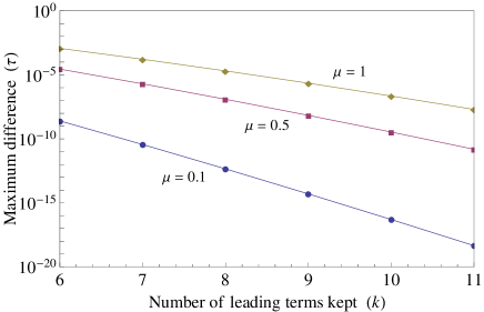
Figure 2: (Color Online) Upper bounds on the dropped terms in Eq. (10). It can be seen that the effect of dropping higher order terms is negligible when the number of leading terms kept, $k$, is not too small.

We follow the statistical fluctuation analysis proposed in Ref. Ma et al. (2005). Then, the equalities in Eq. (10) becomes inequalities,

$$\hat{Q}_{\mu_{k}\nu_{l}}^{w}(1-\beta_{q}) \leq\sum_{i,j}\frac{\mu_{k}^{i}\nu_{l}^{j}}{i!j!}e^{-\mu_{k}-\nu_{l}}Y_{ij}^{w}\leq\hat{Q}_{\mu_{k}\nu_{l}}^{w}(1+\beta_{q})$$ (11)

$$\hat{E}_{\mu_{k}\nu_{l}}^{w}\hat{Q}_{\mu_{k}\nu_{l}}^{w}(1-\beta_{eq}) \leq\sum_{i,j}\frac{\mu_{k}^{i}\nu_{l}^{j}}{i!j!}e^{-\mu_{k}-\nu_{l}}e_{ij}^{w}Y_{ij}^{w}\leq\hat{E}_{\mu_{k}\nu_{l}}^{w}\hat{Q}_{\mu_{k}\nu_{l}}^{w}(1+\beta_{eq}),$$

where if the left hand side of the inequality is negative, we replace it with 0. The variables, $\hat{Q}_{\mu_{k}\nu_{l}}^{w}$ and $\hat{E}_{\mu_{k}\nu_{l}}^{w}$ are measurement outcomes. That is, they are rates instead of probabilities. The fluctuation ratio $\beta_{q}$ and $\beta_{eq}$ can be evaluated by

$$\beta_{q} =\frac{n_{\alpha}}{\sqrt{N_{\mu_{k}\nu_{l}}^{w}\hat{Q}_{\mu_{k}\nu_{l}}^{w}}},$$ (12)

$$\beta_{eq} =\frac{n_{\alpha}}{\sqrt{N_{\mu_{k}\nu_{l}}^{w}\hat{E}_{\mu_{k}\nu_{l}}^{w}\hat{Q}_{\mu_{k}\nu_{l}}^{w}}},$$

where $N_{\mu_{k}\nu_{l}}^{w}$ is the number of pulses, in the $w$ basis, sent out by Alice and Bob when they use intensities $\mu_{k}$ and $\nu_{l}$, respectively; $n_{\alpha}$ is the number of standard deviations one chooses for statistical fluctuation analysis. In other words, $N_{\mu_{k}\nu_{l}}^{w}\hat{Q}_{\mu_{k}\nu_{l}}^{w}$ is the number of successful partial BSMs when Alice and Bob use intensities $\mu_{k}$ and $\nu_{l}$, respectively, and $N_{\mu_{k}\nu_{l}}^{w}\hat{E}_{\mu_{k}\nu_{l}}^{w}\hat{Q}_{\mu_{k}\nu_{l}}^{w}$ is the corresponding error count. If we follow the Gaussian assumption made in Ma et al. (2005), the number of standard deviations, $n_{\alpha}$, will be directly related to the failure probability of this security analysis. For example, when $n_{\alpha}=5$, as used later, it will introduce a failure probability of $5.73\times 10^{-7}$.

V Simulation

For simplicity, we assume that Alice and Bob send the same number of pulses for all $\mu\uplus\nu$ channels, denoted by $N_{data}$. In the following simulations, the parameters of the experimental setup are listed in Table 1.

$e_{d}$	$p_{d}$	$f$	$N_{data}$
1.5%	$3\times 10^{-6}$	1.16	$2\times 10^{10}$

Table 1: List of experimental parameters used in numerical results: $e_{d}$ is the misalignment probability; $p_{d}$ is the background count rate per detector; $f$ is the error correction inefficiency; $N_{data}$ is the number of pulses sent by Alice and Bob for each pair of intensities.

In the simulation, we absorb the detection loss into channel losses. Note that with the current development in high-speed QKD systems Yuan et al. (2007); Sasaki et al. (2011); Wang et al. (2012), $N_{data}=2\times 10^{10}$ pulses can be transmitted in seconds. We assume that Alice and Bob pick $n_{\alpha}$ standard deviations for the statistical fluctuation analysis, which is determined by the allowable failure probability for the system.

V.1 Vacuum+weak-decoy-state protocol

We consider that Alice and Bob run the vacuum+weak-decoy-state protocol Ma et al. (2005) and they choose the same intensities for the coherent states. Let us assume a typical set of intensities: $\{0,0.1,0.5\}$. Note that we assume $N_{data}=2\times 10^{10}$ for each $\mu\uplus\nu$ channel. Thus, the total number of pulses sent by Alice and Bob is $18\times 10^{10}$.

For each of the nine $\mu\uplus\nu$ channels, Alice and Bob can obtain a set of linear inequalities, in the form of Eq. (11), for gains and QBERs. As noted before, we neglect terms with $i,j\geq 7$, and find the lower bound on $Y_{11}^{z}$ and the upper bound on $e_{11}^{x}$ using linear programming.

In order to obtain a sense of the magnitude of the parameter values, we calculate the gains and QBERs, at $\eta_{a}=\eta_{b}=0.1$, using Eqs. (2) and (III.2) for the $x$ and $z$ basis. The gain values are listed in Table 2.

	z-basis			x-basis
Bob/Alice	$\mu=0$	$\mu=0.1$	$\mu=0.5$	$\mu=0$	$\mu=0.1$	$\mu=0.5$
$\nu=0$	$3.6000\times 10^{-11}$	$5.9587\times 10^{-8}$	$2.8900\times 10^{-7}$	$3.5999\times 10^{-11}$	$2.4873\times 10^{-5}$	$6.0229\times 10^{-4}$
$\nu=0.1$	$5.9587\times 10^{-8}$	$4.9374\times 10^{-5}$	$2.3935\times 10^{-4}$	$2.4873\times 10^{-5}$	$9.8876\times 10^{-5}$	$8.6437\times 10^{-4}$
$\nu=0.5$	$2.8900\times 10^{-7}$	$2.3935\times 10^{-4}$	$1.1603\times 10^{-3}$	$6.0229\times 10^{-4}$	$8.6437\times 10^{-4}$	$2.3495\times 10^{-3}$

Table 2: Simulation values of the gain, $Q_{\mu\nu}^{w}$, $w=x,z$, for the vacuum+weak-decoy-state protocol, evaluated using Eqs. (2) and (III.2). It is assumed that $\eta_{a}=\eta_{b}=0.1$.

The QBER of the case when either party chooses the vacuum decoy state is 1/2 and that of the remaining four nontrivial cases is shown in Table 3, for the $x$ and $z$ basis. Note that the QBER in the $z$ basis is reasonably close to $e_{d}$ as expected from Eqs. (III.2) and (7). The QBER in the $x$ basis, on the other hand, is larger than 25%, which is mainly caused by false triggering of multiphoton states Lo et al. (2012); Ma and Razavi (2012). This is the key reason why the final key in Eq. (8) should be only extracted from the $z$ basis.

	z-basis		x-basis
Bob/Alice	$\mu=0.1$	$\mu=0.5$	$\mu=0.1$	$\mu=0.5$
$\nu=0.1$	$1.6164\%$	$1.5700\%$	$25.7184\%$	$36.3867\%$
$\nu=0.5$	$1.5700\%$	$1.5236\%$	$36.3867\%$	$25.4516\%$

Table 3: Simulation values of QBER, $E_{\mu\nu}^{w}$, $w=x,z$, for different intensity values evaluated from Eqs. (2) and (III.2).

In practice, $\hat{Q}_{\mu\nu}^{w}$ and $\hat{E}_{\mu\nu}^{w}$, similar to those in Tables 2 and 3, are derived from the raw data obtained in the experiment. The task of the security analysis, which is the main focus of this work, is to determine the final secure key rate for such sets of data. Following the analysis given in Sec. IV.2, here we minimize $Y_{11}^{z}$ and maximize $e_{11}^{x}$ subject to constraints of Eq. (11), by assuming that the values listed in Tables 2 and 3 are, respectively, the measured gain and QBER in a certain experiment.

Table 4 provides lower and upper bounds on these parameters, obtained by solving the corresponding linear-programming problems, and compared them with the expected values from the simulation results of Eq. (7). From Table 4, one can see that the parameter estimations in the $x$ basis is worse than those in the $z$ basis. This is because multiphoton terms contribute more to the gains and QBERs in the $x$ basis than in the $z$ basis.

		$w=z$		$w=x$
Parameters	Asymptotic value	Lower bound	Upper bound	Lower bound	Upper bound
$Y_{11}^{w}$	$5.0011\times 10^{-3}$	$4.6043\times 10^{-3}$	$6.0286\times 10^{-3}$	$4.1343\times 10^{-3}$	$6.6334\times 10^{-3}$
$e_{11}^{w}$	$1.5108\%$	$0.9556\%$	$2.1341\%$	$0$	$10.2126\%$

Table 4: Lower and upper bounds on $Y_{11}^{w}$ and $e_{11}^{w}$ in both bases, compared to asymptotic values. In our statistical fluctuation analysis, five standard deviations are taken into consideration.

Substituting the parameter estimations from Table 4, the lower bound of $Y_{11}^{z}$ and the upper bound of $e_{11}^{x}$, into Eq. (8), one can calculate the key rate to be $6.89\times 10^{-5}$ bits/pulse. Similarly, one can evaluate the dependence of the key rate on channel transmittance, as shown in Fig. 3. One can see that even by including statistical fluctuations the key rate decreases linearly with channel loss before the cut-off regime. In the low-loss regime, the vacuum+weak-decoy-state protocol performs almost as well as the asymptotic case.

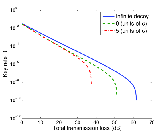
Figure 3: Key rate versus channel transmittance using vacuum+weak decoy-state method for MDI-QKD.

As shown in Fig. 3, with $n_{\alpha}=5$ standard deviations, the maximum tolerable transmission loss is almost 30 dB less than that of the asymptotic case. Even if we do not take the statistical fluctuations ($n_{\alpha}=0$) into account, there is still a gap between the two cases. Thus, there is big room for further improvement. In the next simulation, we will consider three decoy states and show that further improvements can be made when more decoy states are applied.

V.2 Vacuum+two-weak-decoy-state protocol

In order to give a better estimation of $Y_{11}^{z}$ and $e_{11}^{x}$, one can use more than two decoy states. Let us assume that Alice and Bob use four coherent states $\{0,0.1,0.2,0.5\}$ and that we use $N_{data}=2\times 10^{10}$ for each $\mu\uplus\nu$ channel. Thus, the total number of pulses sent by Alice and Bob is $32\times 10^{10}$, corresponding to 16 channels. Given that by adding an extra decoy state on each side we can better estimate channel parameters, the key rate is expected to be no less than the one in Sec. V.1.

Similar to the previous section, we take $\eta_{a}=\eta_{b}=0.1$ as an example to see how accurate the parameter estimation is. The bounds of $Y_{11}^{z}$ and $e_{11}^{x}$ in both bases, compared to the asymptotic case, are listed in Table 5. Again, the parameter estimations in the $x$ basis is worse than those in the $z$ basis, due to the multiphoton terms.

		$w=z$		$w=x$
Parameters	Asymptotic value	Lower bound	Upper bound	Lower bound	Upper bound
$Y_{11}^{w}$	$5.0011\times 10^{-3}$	$4.7058\times 10^{-3}$	$5.2377\times 10^{-3}$	$4.3734\times 10^{-3}$	$5.5640\times 10^{-3}$
$e_{11}^{w}$	$1.5108\%$	$1.1103\%$	$2.0409\%$	$0$	$7.7954\%$

Table 5: Lower and upper bounds on $Y_{11}^{w}$ and $e_{11}^{w}$ in both bases, compared to asymptotic values. In our statistical fluctuation analysis, five standard deviations are taken into consideration.

Similar to the vacuum+weak-decoy-state case, one can calculate the key rate to be $1.09\times 10^{-4}$ bits/pulse by substituting the parameter estimations from Table 5, the lower bound of $Y^{z}_{11}$ and the upper bound of $e^{x}_{11}$, into Eq. (8). According to Table 5, our parameter estimation has improved when more decoy states (in extra pulses) are applied, as compared to the previous case in Table 4.

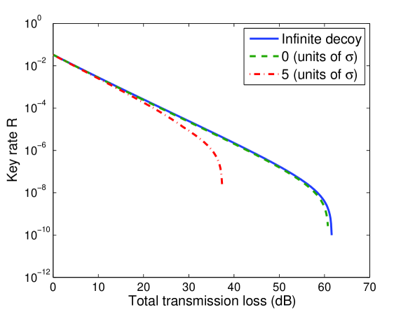
Figure 4: Key rate versus channel transmittance using vacuum+two-weak-decoy-state method for MDI-QKD.

The dependence of the key rate on the channel transmittance is shown in Fig. 4. One can see that the gap between the finite-size case and the asymptotic case is smaller than the one shown in Fig. 3. In the case of $n_{\alpha}=0$, the vacuum+two-weak-decoy-state protocol is very close to the asymptotic case. This is different from regular decoy-state protocol, where two decoy states are proven to be sufficient for practical usage Ma et al. (2005).

VI Conclusions

We showed that MDI-QKD is a highly practical scheme even when the statistical fluctuations are accounted for. In the low-loss regime, with only two or three decoy states, the performance of MDI-QKD with statistical fluctuations is close to that of the asymptotic case. At higher values of loss, using three decoy states would be recommended. We remark that our analysis is quite general and is applicable to different MDI-QKD implementations such as those based on phase encoding and/or polarization encoding as well as those those based on the BB84 protocol or the six-state protocol.

References

- Bennett and Brassard (1984) C. H. Bennett and G. Brassard, in Proceedings of IEEE International Conference on Computers, Systems, and Signal Processing (IEEE, New York, Bangalore, India, 1984) pp. 175–179.
- Ekert (1991) A. K. Ekert, Phys. Rev. Lett. , 67, 661 (1991).
- Mayers (2001) D. Mayers, Journal of the ACM (JACM), 48, 351 (2001).
- Lo and Chau (1999) H.-K. Lo and H. F. Chau, Science, 283, 2050 (1999).
- Shor and Preskill (2000) P. W. Shor and J. Preskill, Phys. Rev. Lett. , 85, 441 (2000).
- Biham et al. (2000) E. Biham, M. Boyer, P. O. Boykin, T. Mor, and V. Roychowdhury, in Proc. of the Thirty-Second Annual ACM Symposium on Theory of Computing (ACM Press, New York, 2000) pp. 715–724.
- Inamori et al. (2007) H. Inamori, N. Lütkenhaus, and D. Mayers, Eur. Phys. J. D, 41, 599 (2007).
- Renner et al. (2005) R. Renner, N. Gisin, and B. Kraus, Phys. Rev. A, 72, 012332 (2005).
- Beaudry et al. (2008) N. J. Beaudry, T. Moroder, and N. Lütkenhaus, Phys. Rev. Lett., 101, 093601 (2008).
- Tsurumaru and Tamaki (2008) T. Tsurumaru and K. Tamaki, Phys. Rev. A, 78, 032302 (2008).
- Fung et al. (2011) C.-H. F. Fung, H. F. Chau, and H.-K. Lo, Phys. Rev. A, 84, 020303 (2011).
- Gottesman et al. (2004) D. Gottesman, H.-K. Lo, N. Lütkenhaus, and J. Preskill, Quant. Inf. Comput., 4, 325 (2004).
- Makarov et al. (2006) V. Makarov, A. Anisimov, and J. Skaar, Phys. Rev. A, 74, 022313 (2006).
- Makarov and Skaar (2008) V. Makarov and J. Skaar, Quant. Inf. Comput. , 8, 0622 (2008).
- Qi et al. (2007) B. Qi, C.-H. F. Fung, H.-K. Lo, and X. Ma, Quant. Inf. Comput., 7, 073 (2007).
- Zhao et al. (2008) Y. Zhao, C.-H. F. Fung, B. Qi, C. Chen, and H.-K. Lo, Phys. Rev. A, 78, 042333 (2008).
- Fung et al. (2007) C.-H. F. Fung, B. Qi, K. Tamaki, and H.-K. Lo, Phys. Rev. A, 75, 032314 (2007).
- (18) F. Xu, B. Qi, and H.-K. Lo, New Journal of Physics, 12, 113026.
- Lydersen et al. (2010) L. Lydersen, C. Wiechers, C. Wittmann, D. Elser, J. Skaar, and V. Makarov, Nature photonics, 4, 686 (2010).
- Gerhardt et al. (2011) I. Gerhardt, Q. Liu, A. Lamas-Linares, J. Skaar, C. Kurtsiefer, and V. Makarov, Nature Communications, 2, 349 (2011).
- Fung et al. (2009) C.-H. F. Fung, K. Tamaki, B. Qi, H.-K. Lo, and X. Ma, Quant. Inf. Comput., 9, 0131 (2009).
- Lydersen and Skaar (2010) L. Lydersen and J. Skaar, Quant. Inf. Comput., 10, 0060 (2010).
- Marøy et al. (2010) O. Marøy, L. Lydersen, and J. Skaar, Phys. Rev. A, 82, 032337 (2010).
- Mayers and Yao (1998) D. Mayers and A. Yao, in FOCS, 39th Annual Symposium on Foundations of Computer Science (IEEE, Computer Society Press, Los Alamitos, 1998) p. 503.
- Acín et al. (2007) A. Acín, N. Brunner, N. Gisin, S. Massar, S. Pironio, and V. Scarani, Physical Review Letters, 98, 230501 (2007).
- Pironio et al. (2009) S. Pironio, A. Acin, N. Brunner, N. Gisin, S. Massar, and V. Scarani, New Journal of Physics, 11, 045021 (25pp) (2009).
- Bell (1964) J. S. Bell, Physics, 1, 195 (1964).
- Clauser et al. (1969) J. F. Clauser, M. A. Horne, A. Shimony, and R. A. Holt, Phys. Rev. Lett., 23, 880 (1969).
- Pearle (1970) P. M. Pearle, Phys. Rev. D, 2, 1418 (1970).
- Garg and Mermin (1987) A. Garg and N. D. Mermin, Phys. Rev. D, 35, 3831 (1987).
- Ma and Lütkenhaus (2012) X. Ma and N. Lütkenhaus, Quant. Inf. Comput., 12, 0203 (2012).
- Pawłowski and Brunner (2011) M. Pawłowski and N. Brunner, Phys. Rev. A, 84, 010302 (2011).
- Lo et al. (2012) H.-K. Lo, M. Curty, and B. Qi, Phys. Rev. Lett., 108, 130503 (2012).
- Biham et al. (1996) E. Biham, B. Huttner, and T. Mor, Phys. Rev. A, 54, 2651 (1996).
- Inamori (2002) H. Inamori, Algorithmica, 34, 340 (2002).
- Braunstein and Pirandola (2012) S. L. Braunstein and S. Pirandola, Phys. Rev. Lett., 108, 130502 (2012).
- Tamaki et al. (2012) K. Tamaki, H.-K. Lo, C.-H. F. Fung, and B. Qi, Phys. Rev. A, 85, 042307 (2012).
- Ma and Razavi (2012) X. Ma and M. Razavi, Arxiv preprint arXiv:1204.4856 (2012).
- Rubenok et al. (2012) A. Rubenok, J. Slater, P. Chan, I. Lucio-Martinez, and W. Tittel, Arxiv preprint arXiv:1204.0738 (2012).
- da Silva et al. (2012) T. da Silva, D. Vitoreti, G. Xavier, G. Temporão, and J. von der Weid, Arxiv preprint arXiv:1207.6345 (2012).
- Liu et al. (2012) Y. Liu, T.-Y. Chen, L.-J. Wang, H. Liang, G.-L. Shentu, J. Wang, K. Cui, H.-L. Yin, N.-L. Liu, L. Li, X. Ma, J. S. Pelc, M. M. Fejer, Q. Zhang, and J.-W. Pan, Arxiv preprint arXiv:1209.6178 (2012).
- Hwang (2003) W.-Y. Hwang, Phys. Rev. Lett. , 91, 057901 (2003).
- Lo et al. (2005) H.-K. Lo, X. Ma, and K. Chen, Phys. Rev. Lett. , 94, 230504 (2005).
- Ma et al. (2005) X. Ma, B. Qi, Y. Zhao, and H.-K. Lo, Phys. Rev. A, 72, 012326 (2005).
- Wang (2005) X.-B. Wang, Phys. Rev. Lett. , 94, 230503 (2005a).
- Wang (2005) X.-B. Wang, Phys. Rev. A, 72, 012322 (2005b).
- Song et al. (2012) T.-T. Song, Q.-Y. Wen, F.-Z. Guo, and X.-Q. Tan, Phys. Rev. A, 86, 022332 (2012).
- Bruß (1998) D. Bruß, Phys. Rev. Lett., 81, 3018 (1998).
- Koashi and Preskill (2003) M. Koashi and J. Preskill, Phys. Rev. Lett. , 90, 057902 (2003).
- Ma (2008) X. Ma, Quantum cryptography: from theory to practice, Ph.D. thesis, University of Toronto (2008), also available in arXiv:0808.1385.
- Note (1) To upper bound , we divide the upper bound of with the lower bound of .
- Yuan et al. (2007) Z. Yuan, B. Kardynal, A. Sharpe, and A. Shields, Applied Physics Letters, 91, 041114 (2007).
- Sasaki et al. (2011) M. Sasaki, M. Fujiwara, H. Ishizuka, W. Klaus, K. Wakui, M. Takeoka, A. Tanaka, K. Yoshino, Y. Nambu, S. Takahashi, A. Tajima, A. Tomita, T. Domeki, T. Hasegawa, Y. Sakai, H. Kobayashi, T. Asai, K. Shimizu, T. Tokura, T. Tsurumaru, M. Matsui, T. Honjo, K. Tamaki, H. Takesue, Y. Tokura, J. F. Dynes, A. R. Dixon, A. W. Sharpe, Z. L. Yuan, A. J. Shields, S. Uchikoga, M. Legre, S. Robyr, P. Trinkler, L. Monat, J.-B. Page, G. Ribordy, A. Poppe, A. Allacher, O. Maurhart, T. Langer, M. Peev, and A. Zeilinger, Opt. Exp., 19, 10387 (2011).
- Wang et al. (2012) S. Wang, W. Chen, J.-F. Guo, Z.-Q. Yin, H.-W. Li, Z. Zhou, G.-C. Guo, and Z.-F. Han, Opt. Lett., 37, 1008 (2012).