Analysis of Spitzer-IRS spectra of hyperluminous infrared galaxies

Abstract

Context. Hyperluminous infrared galaxies (HLIRG) are the most luminous persistent objects in the Universe. They exhibit extremely high star formation rates, and most of them seem to harbour an Active Galactic Nucleus (AGN). They are unique laboratories to investigate the most extreme star formation, and its connection to super-massive black hole growth.

Aims. The AGN and starburst (SB) relative contributions to the total output in these objects is still debated. Our aim is to disentangle the AGN and SB emission of a sample of thirteen HLIRG.

Methods. We have studied the MIR low resolution spectra of a sample of thirteen HLIRG obtained with the Infrared Spectrograph on board Spitzer. The $5-8$ $\upmu$m range is an optimal window to detect AGN activity even in a heavily obscured environment. We performed a SB/AGN decomposition of the continuum using templates, which has been successfully applied for ULIRG in previous works.

Results. The MIR spectra of all sources is largely dominated by AGN emission. Converting the 6 $\upmu$m luminosity into IR luminosity, we found that $\sim 80\%$ of the sample shows an IR output dominated by the AGN emission. However, the SB activity is significant in all sources (mean SB contribution $\sim 30\%$), showing star formation rates $\sim 300-3000\leavevmode\nobreak\ M_{\mathrm{\sun}}\mathrm{yr}^{-1}$. Using X-ray and MIR data we estimated the dust covering factor (CF) of these HLIRG, finding that a significant fraction presents a CF consistent with unity. Along with the high X-ray absorption shown by these sources, this suggests that large amounts of dust and gas enshroud the nucleus of these HLIRG, as also observed in ULIRG.

Conclusions. Our results are in agreement with previous studies of the IR SED of HLIRG using radiative transfer models, and we find strong evidence that all HLIRG harbour an AGN. Moreover, this work provides further support to the idea that AGN and SB are both crucial to understand the properties of HLIRG. Our study of the CF supports the hypothesis that HLIRG can be divided in two different populations.

1 Introduction

One of the most important results brought by the Infrared Astronomical Satellite (IRAS) was the detection of a new class of galaxies where the bulk of their bolometric emission lies in the infrared range (Soifer et al. 1984b). This population, named luminous infrared galaxies (LIRG), becomes the dominant extragalactic population at IR luminosities above $10^{11}L_{\mathrm{\sun}}$, with a space density higher than all other classes of galaxies of comparable bolometric luminosity (see Sanders & Mirabel 1996 for a complete review of these objects). At the brightest end of this population distribution lie the ultraluminous (ULIRG; $L_{\mathrm{IR}}>10^{12}\leavevmode\nobreak\ L_{\mathrm{\sun}}$) and the hyperluminous infrared galaxies (HLIRG; $L_{\mathrm{IR}}>10^{13}\leavevmode\nobreak\ L_{\mathrm{\sun}}$).

Ever since the discovery of LIRG two possible origins have been suggested for the observed luminosities: Active Galactic Nuclei (AGN) and/or stellar formation in starburst (SB) episodes (Rieke et al. 1980; Soifer et al. 1984a; Wright et al. 1984; Soifer et al. 1987a; Carico et al. 1990; Condon et al. 1991). The AGN/SB relative contributions to the IR output of this kind of sources shows a clear trend with luminosity: while LIRG and low-luminosity ULIRG are SB-dominated sources, the AGN emission is essential to explain the bolometric luminosity in high-luminosity ULIRG and HLIRG. The fraction of sources harbouring an AGN and its relative contribution increases with IR luminosity (Veilleux et al. 1999; Rowan-Robinson 2000; Tran et al. 2001; Farrah et al. 2002a; Veilleux et al. 2002; Farrah et al. 2006; Nardini et al. 2010).

Understanding the ultimate physical mechanism which triggers those phenomena and, particularly in those sources with extreme IR luminosities, their interplay, is crucial to obtain a complete view of galaxy evolution. Over the last decade comprehensive observations from X-rays to radio have produced a consistent paradigm for local ULIRG. Now is broadly accepted that these objects are dusty galaxies where fierce star formation processes have been triggered by mergers or interactions between gas-rich galaxies (Mihos & Hernquist 1994; Genzel et al. 2001; Dasyra et al. 2006). Only half of them harbour an AGN, which usually is a minor contributor to the total IR emission (cf. Lonsdale et al. 2006, for a complete review).

ULIRG are rare in the Local Universe (Soifer et al. 1987b), but a large number has been detected instead in deep-IR surveys, being a fundamental constituent of the high-redshift galaxy population (Franceschini et al. 2001; Elbaz et al. 2002; Lonsdale et al. 2004; Daddi et al. 2005; Farrah et al. 2006; Caputi et al. 2007; Magdis et al. 2010, 2011). It has been proposed that ULIRG at high redshift could be at the origin of massive elliptical and S0 galaxies (Franceschini et al. 1994; Lilly et al. 1999; Genzel & Cesarsky 2000; Genzel et al. 2001). A large fraction of stars in present-day galaxies would have been formed during these evolutionary phases. However, the paradigm described above is not so well-grounded for the high-$z$ ULIRG population (Rodighiero et al. 2011; Draper & Ballantyne 2012; Niemi et al. 2012), neither for higher luminosity objects like HLIRG.

HLIRG seem to be composite sources, i.e. AGN and SB phenomena are both needed to fully explain their IR emission (Rowan-Robinson 2000; Farrah et al. 2002a; Ruiz et al. 2010; Rowan-Robinson & Wang 2010; Han & Han 2012), and only about a third has been found in interacting systems (Farrah et al. 2002b). This suggests that most HLIRG are not triggered by mergers, as also found for a significant number of high-$z$ ULIRG (Sturm et al. 2010; Draper & Ballantyne 2012; Niemi et al. 2012). If HLIRG and high-$z$ ULIRG share other properties, local HLIRG, since they are brighter and easier to study with the current astronomical tools, could be key objects to understand the high-$z$ population of ULIRG. Moreover, as HLIRG could represent the most vigorous stage of galaxy formation, with SFR $>1000\leavevmode\nobreak\ M_{\mathrm{\sun}}\mathrm{yr}^{-1}$, they are unique laboratories to investigate extremely high stellar formation, and its connection to super-massive black hole (SMBH) growth.

The relative contributions of AGN and SB to the bolometric luminosity of HLIRG is still in debate. Early studies of small samples of HLIRG found contradictory results, with some authors suggesting that the IR emission arises predominantly from a SB (Frayer et al. 1998, 1999) with star formation rates (SFR) of the order $1000\leavevmode\nobreak\ \mathrm{M_{\mathrm{\sun}}yr}^{-1}$, and other authors suggesting that HLIRG are powered by a dusty AGN (Granato et al. 1996; Evans et al. 1998; Yun & Scoville 1998). The analysis of the IR Spectral Energy Distributions (SED) of larger samples of HLIRG revealed that about half of these sources are AGN-dominated (Rowan-Robinson 2000; Verma et al. 2002; Rowan-Robinson & Wang 2010). Our analysis of the HLIRG’s broadband (from radio to X-rays) SED (Ruiz et al. 2010) obtained consistent results, showing that both AGN and SB components are needed to reproduce the full emission of these objects, being the bolometric luminosity of the AGN dominant, or at least comparable to the SB luminosity, in $\sim 70\%$ of the studied HLIRG. These studies were however based on samples biased toward AGN.

Farrah et al. 2002a (hereafter F02) built a sample of HLIRG with a negligible bias toward AGN and it was observed with the Submillimetre Common-User Bolometer Array (SCUBA; Holland et al. 1999). Submillimetre data introduced tight constraints on SB luminosities in the IR SED analysis. They found most HLIRG being AGN-dominated sources, but with a significant contribution ($\gtrsim 20\%$) due to star formation in all objects.

In Ruiz et al. (2007) we tried to disentangle the AGN and SB emission of HLIRG following a different approach. Since the 2-10 keV X-ray emission above $\sim 10^{42}\leavevmode\nobreak\ \mathrm{erg\leavevmode\nobreak\ s^{-1}}$ is the “smoking gun” of AGN activity (Mushotzky 2004), we studied the X-ray spectra of a sample of fourteen HLIRG observed by XMM-Newton. We found that all the detected sources (ten out of fourteen) were AGN-dominated in the X-ray band, but most were underluminous in X-rays with respect to the predicted luminosity by the standard AGN SED from Risaliti & Elvis (2004), given their IR luminosities. We also found strong evidence that a significant fraction of these objects is heavily obscured, reaching the Compton Thick level (hydrogen column, $N_{\mathrm{H}}$ $>10^{24}\leavevmode\nobreak\ \mathrm{cm}^{-2}$), as suggested by previous studies (Wilman et al. 2003; Iwasawa et al. 2005). Such absorption level allows, in the best cases, only the detection of reflected X-ray emission. To avoid the strong obscuration effects and in order to obtain a more complete and independent view of these sources, we need to move to another spectral window.

In this paper we present a study of a sample of HLIRG in the Mid-Infrared (MIR) band, $\lambda=5-8$ $\upmu$m, a spectral range very efficient in detecting AGN emission and less affected by absorption than X-rays. Several diagnostic methods are available to unravel the AGN and SB activity through the MIR spectra, e.g. the study of high-ionization emission lines and the polycyclic aromatic hydrocarbon (PAH) features (Laurent et al. 2000; Armus et al. 2007; Spoon et al. 2007; Farrah et al. 2007) or the analysis of the continuum around 4 $\upmu$m (Risaliti et al. 2006). Blind statistical techniques, like principal component analysis, have been also successfully employed with MIR spectra (Wang et al. 2011; Hurley et al. 2012). However, given the limited size of our sample, we cannot apply such statistical methods.

The MIR continuum of pure AGN and pure SB show small dispersion below 10 $\upmu$m (Netzer et al. 2007; Brandl et al. 2006), allowing the use of universal templates to reproduce the AGN and SB emission in sources where both physical processes are present. Hence, we can unravel the AGN and SB components of composite sources modelling their MIR spectra with such templates. The key reason for using the continuum emission at $\lambda\simeq 5-8$ $\upmu$m as a diagnostic is the difference of the 6 $\upmu$m-to-bolometric ratios between AGN and SB (approximately two orders of magnitude larger in the former). This makes the detection of the AGN component possible even when the AGN is heavily obscured and/or bolometrically weak compared to the SB.

SB/AGN continuum spectral decomposition has been successfully applied in ULIRG (Nardini et al. 2008, 2009, 2010; Risaliti et al. 2010) to disentangle the emission of both components. A significant number of HLIRG has been observed with the Infrared Spectrograph (IRS, Houck et al. 2004) on board Spitzer (Werner et al. 2004), obtaining good quality spectra to apply this diagnostic technique.

The outline of the paper is as follows: Section 2 describes the selected sample of HLIRG. The IRS data reduction is explained in Sect. 3. In Sect. 4 we explain the decomposition process, the model adopted and the results obtained. Section 5 discuss the results of the MIR spectral analysis and Sect. 6 summarizes our conclusions.

The Wilkinson Microwave Anisotropy Probe (WMAP) concordance cosmology has been adopted along the paper: $H_{0}=70$ km s^-1 Mpc^-1, $\Omega_{m}=0.27,\Omega_{\Lambda}=0.73$ (Komatsu et al. 2009).

2 The sample

This paper is based on the analysis of the F02 sample of HLIRG. Nine out of ten sources in that sample have been observed with the Spitzer-IRS in its low-resolution mode and the data are publicly available in the Spitzer Archive.

The F02 sample was originally selected in a manner independent of obscuration, inclination or AGN content. Moreover, its parent sample is composed by objects found from direct optical follow-up of 60 $\upmu$m or 850 $\upmu$m surveys (Rowan-Robinson 2000) and hence it is statistically homogeneous and complete.

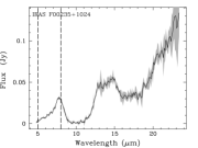
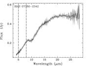
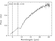
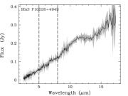
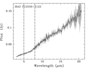
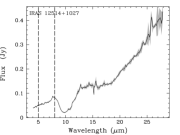
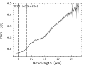
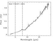
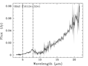
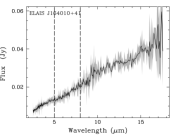
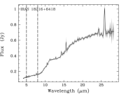
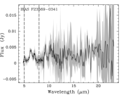
Figure 1: MIR rest-frame spectra of HLIRG obtained with the Infrared Spectrograph onboard Spitzer. The grey shaded area is the $1\sigma$ uncertainty region. The vertical dashed lines limit the spectral region where our decomposition technique was applied.

Given these selection criteria, F02 claim that the sample should be entirely free from AGN bias. However, since the parent sample is composed of sources selected from surveys at different wavelenghts, this could produce significant biases in favour or against ’hot’ dust, which is more common in AGN than in SB (de Grijp et al. 1985; Soifer et al. 1987a). Thus, objects from 60 $\upmu$m surveys are more likely to contain hot dust heated by AGN, while those sources from 850 $\upmu$m surveys will be biased towards cold dust heated by star formation. However, we must note that only a small fraction of the Rowan-Robinson (2000) sample is selected from 850 $\upmu$m data (less than $10\%$), and a similar fraction is found in the F02 sample. Moreover, the effect of the AGN hot dust in composite sources with equal AGN and SB bolometric output is severely diminished beyond $\sim 30$ $\upmu$m rest-frame (cf. Fig. 1 of Nardini et al. 2009). Only three HLIRG in the F02 sample are at $z\sim 1$, so the effect of hot dust is minimal. The potential AGN bias is therefore negligible and we consider the F02 sample suitable for drawing global conclusions about the HLIRG population.

Only five sources of this sample have been observed by XMM-Newton, and just two of these five HLIRG were detected (Ruiz et al. 2007). In order to study the relation between the X-ray and MIR emission for this kind of sources, we included four additional HLIRG to our sample. These objects were selected from the X-ray-selected HLIRG sample we analysed in Ruiz et al. (2007). They all were detected by XMM-Newton and observed with Spitzer-IRS. Three of these additional HLIRG were found via comparisons to known AGN (Tables 2-4 of Rowan-Robinson 2000) and therefore its inclusion leads to a non-negligible bias toward AGN content in our final sample. Nevertheless, in some ocassions we can derive conclusions about the global population of HLIRG restricting our results to the F02 sample (nine out of ten F02 sources are included in our sample).

There are thirteen HLIRG in our final sample. Accordingly to their optical spectra, six are type 1 AGN (Seyfert 1 or QSO), four are type 2 AGN (Seyfert 2 or QSO2) and three are SB galaxies (see Table 1). The IR SED of all sources have been observed and studied using radiative transfer models (RTM) through several papers (F02; Rowan-Robinson 2000; Verma et al. 2002). AGN and SB components are both needed to reproduce the IR emission of these HLIRG, the AGN output being dominant in most sources (eight out of thirteen).

Regarding only to the objects in the F02 sample, five are type 1 AGN and four are optically classified as narrow-line (NL) objects. All type 1 sources and one NL object show an AGN-dominated IR SED, and the remaining (three) NL sources show an SB-dominated IR SED, accordingly to the F02 analysis.

The broad band SED (from radio to X-rays) of most sources (nine out of thirteen) have also been studied using observational templates for the AGN and SB components, offering consistent results with those obtained using RTM (Ruiz et al. 2010).

3 Data reduction

All sources from our HLIRG sample have been observed by the IRS onboard Spitzer in the low-resolution mode (see Table 1) and the data were publicly available. All observations were operated in the standard staring mode using the two low-resolution modules (SL and LL). The Basic Calibrated Data (BCD) files, bad pixels masks (BMASK) and flux uncertainty files were downloaded from the Spitzer Heritage Archive v1.5. All files are products of the official Spitzer Science Center pipeline (version S18.18).

The BCD pipeline reduces the raw detector images from individual exposures: removes the electronic and optical artifacts (e.g. dark current, droop effect, non-linear effects, detection of cosmic-ray events), jail-bar pattern and stray light, and perform a flat-field correction. BCD files, along with the corresponding uncertainty images and BMASK files, are reliable inputs for SMART, an IDL-based processing and analysis tool for IRS data (Higdon et al. 2004).

We processed the BCD pipeline files using SMART 8.2.3. We cleaned the BCD files of bad pixels using IRSCLEAN 2.1 and we combined the individual exposures for a given ExpID (uncertainty files were used to perform a weighted-average). In order to remove the background and low-level rogue pixels we subtracted the two observations in the nodding cycle for each module and order (SL1, SL2, LL1, LL2). We checked that all sources were point-like and well centered in the slits and finally we ran an automatic, tappered column (window adjusted to the source extent and scaling with wavelength) extraction to obtain the flux and wavelength calibrated spectra. We checked that individual orders did match in flux after extraction, so no further scaling corrections were needed.

Two spectra were obtained for each source, one for each nod. We calculated an error-weighted average of the two nod spectra and they were de-redshifted to rest frame. Figure 1 shows the final spectra.

4 SB/AGN spectral decomposition

4.1 Model for the MIR emission of HLIRG

Thanks to the unprecedent sensitiviy of Spitzer-IRS, MIR studies of large samples of luminous AGN and SB have found a significant spectral homogeneity in the SED of the two separate classes (Brandl et al. 2006; Netzer et al. 2007; Mullaney et al. 2011; Hernán-Caballero & Hatziminaoglou 2011). For high luminosity sources, this is particularly true within the 5-8 $\upmu$m range, showing nearly constants shapes of both the PAH complex in SB (Brandl et al. 2006) and the continuum in AGN (Netzer et al. 2007).

This small spectral dispersion allows the use of universal AGN/SB templates to parameterize the observed energy output of objects where both phenomena are present, like ULIRG or HLIRG, in the wavelength range below 8 $\upmu$m. This technique has been extensively tested in ULIRG, showing that the observed differences of the PAH equivalent width and strength are caused, in most sources, by the relative contribution of the AGN continuum and its obscuration (Nardini et al. 2008, 2009, 2010).

The bolometric luminosities of HLIRG and ULIRG differ no more than about an order of magnitude (even less for the SB component). Moreover, a significant fraction of HLIRG seems to share common properties with local ULIRG (Ruiz et al. 2010). Thus, we can rely with reasonable confidence on the model proposed by Nardini et al. (2008, hereafter N08) to reproduce the 5-8 $\upmu$m emission in HLIRG. The observed flux at wavelength $\lambda$, $f_{\lambda}^{\mathrm{obs}}$, is given by:

$$f_{\lambda}^{\mathrm{obs}}=f_{6}^{\mathrm{int}}\left[\alpha_{6}\leavevmode\nobreak\ u_{\lambda}^{\mathrm{AGN}}\mathrm{e}^{-\tau(\lambda)}+(1-\alpha_{6})\leavevmode\nobreak\ u_{\lambda}^{\mathrm{SB}}\right],$$ (1)

where $\alpha_{6}$ is the AGN contribution to $f_{6}^{\mathrm{int}}$ (the intrinsic flux density at 6 $\upmu$m) while $u_{\lambda}^{\mathrm{AGN}}$ and $u_{\lambda}^{\mathrm{SB}}$ are the AGN and SB emission normalized at 6 $\upmu$m. This model has only three free parameters: $\alpha_{6}$, $\tau_{6}$ (the optical depth at 6 $\upmu$m) and $f_{6}^{\mathrm{int}}$ (the flux normalization). Additional high-ionization emission lines and molecular absorption features (due to ices and aliphatic hydrocarbons), whenever present, were fitted using Gaussian profiles.

Starburst emission

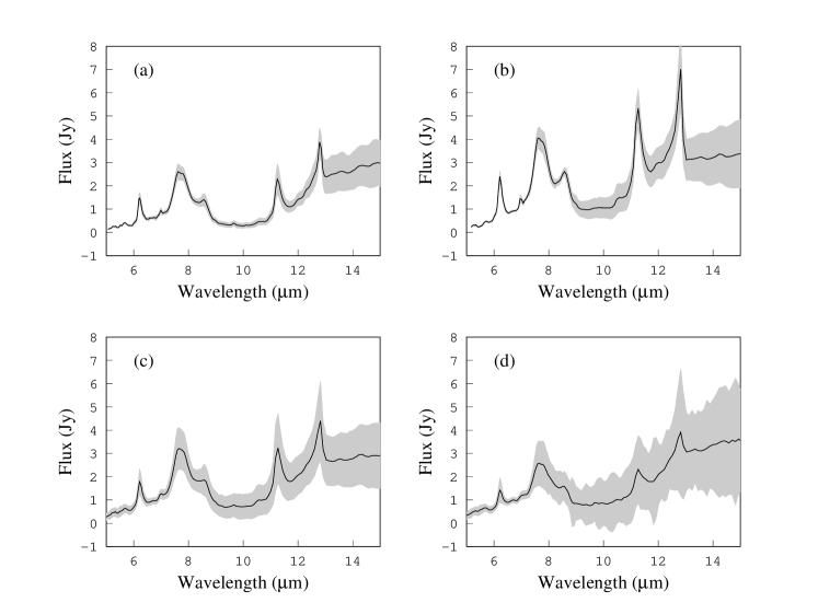
Figure 2: Average SB spectra used as templates in our model: Template (a) is from N08; templates (b), (c) and (d) from Hernán-Caballero & Hatziminaoglou (2011) (see Sect. 4 for details). The grey shaded area is the estimated $1\sigma$ dispersion.

As stated above, starbursts of different luminosities present a small spectral dispersion in their MIR emission below 8 $\upmu$m. Given the large number of physical variables (e.g. the initial mass function, the duration and evolution of the burst, dust grain properties) involved in determining the observational properties of an SB, it is in fact surprising finding such similarity. Brandl et al. (2006) suggested that this homogeneity can derive from the spatial integration of unresolved star-forming spots. We can then assume that an observational template will accurately reproduce the SB emission of our sources in the 5-8 $\upmu$m range. This emission is characterized by two prominent PAH features at 6.2 and 7.7 $\upmu$m (Fig. 2).

To increase the robustness of our analysis we have employed four different SB templates from N08 (a) and from Hernán-Caballero & Hatziminaoglou 2011 (b, c, d): a) the average MIR spectrum from the five brightest ULIRG among pure SB sources in the N08 sample; b) the average spectrum of objects optically classified as SB or HII in NED and with $\nu L_{\nu}$(7 $\upmu$m)$<10^{44}\leavevmode\nobreak\ \mathrm{ergs^{-1}}$ (16 sources); c) the average spectrum of SB-dominated objects in the MIR (257 sources) and d) the average spectrum of objects classified as ULIRG (184 sources). As expected, all SB templates show similar features and small dispersion below 8 $\upmu$m (see Fig. 2).

AGN emission

In our range of interest the AGN spectrum is dominated by the cooling of small dust grains that are transiently heated up to temperatures close to the sublimation limit. This process is expected to produce a nearly featureless power law continuum. However, PAH features are found in several quasars (Schweitzer et al. 2006; Lutz et al. 2007, 2008). Netzer et al. (2007) adscribe the FIR emission of a set of luminous PG QSO to cold dust in extended regions, thus probably of stellar origin. After removing this galactic contamination, the average spectrum can be modeled with a single power law from $\sim 3$ $\upmu$m to the 9.7 $\upmu$m silicate bump. Since the spectral dispersion within this range is small for pure luminous QSO, we can model the AGN emission in our sources with the same power law with a fixed spectral index: $f_{\lambda}\propto\lambda^{0.8}$. Again, to increase the robustness of our results, we alternatively fitted all sources allowing the slope of the power law to vary in the range 0.2-1.8. This interval covers the dispersion found in the spectral index for the AGN emission in ULIRG (Nardini et al. 2010).

Our model includes an exponential attenuation in the AGN emission to take into account the reddening of the NIR radiation due to any compact absorber in the line of sight. The optical depth follows the conventional law $\tau(\lambda)\propto\lambda^{-1.75}$ (Draine 1989). The SB emission does not need a similar correction because the possibles effects of obscuration are already accounted in the observational templates.

4.2 Results

The model presented in the previous section was implemented in Sherpa (Freeman et al. 2001), the modelling and fitting tool included in the software package CIAO 4.3 (Fruscione et al. 2006). The 5-8 $\upmu$m spectra were fitted using a Levenberg-Marquardt $\chi^{2}$ minimization algorithm. The errors of the parameters (within $1\sigma$ confidence limit) were calculated through Montecarlo simulations.

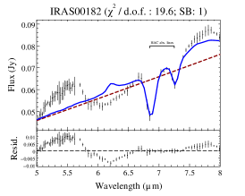
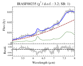
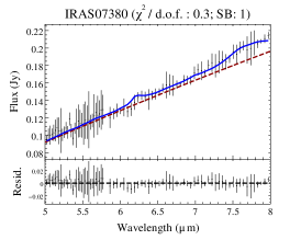
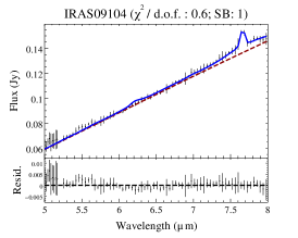
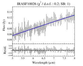
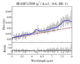
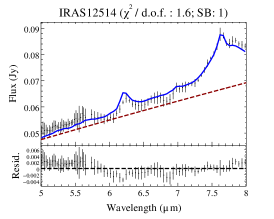
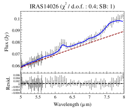
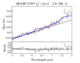
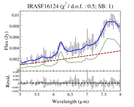
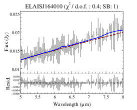
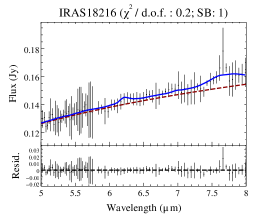
Figure 3: 5-8 $\upmu$m spectra and best fit models (blue solid line). The AGN component is ploted as a red dashed line. For clarity, the SB component (green dotted line) is ploted only on those sources where the AGN and SB contributions are comparable.

One object was barely detected by Spitzer and in two additional sources our model was not suitable (see Sect. 4.3 for a further discussion on these objects), but the spectra of the remaining ten sources were well reproduced by our model (see Fig. 3 and Table 2).

We found no significant difference between the best-fit models using the four SB templates. All templates offer a similar $\chi^{2}$ and consistent values for the model parameters. We have therefore included in Table 2 only the results obtained using the N08 SB template. However, we should note that the use of the ULIRG template provides systematically lower values of $\alpha_{6}$ in all sources. This result is probably caused by the presence of an AGN component in the template, as expected in an average ULIRG spectrum including high-luminosity objects (Nardini et al. 2010; Hernán-Caballero & Hatziminaoglou 2011).

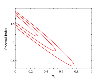
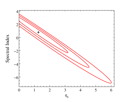
Figure 4: Spectral Index-Optical depth confidence regions for IRAS 07380-2342 (left) and IRAS F16124+3241 (right). The contours represent $1\sigma$, $2\sigma$ and $3\sigma$ confidence levels.

Allowing the spectral index to vary did not enhance the fit in most sources. A statistically significant improvement (in terms of F-test) was found only in three sources with high optical depth (beside IRAS 18216+6418, which is discussed below). However we must note that our model is severely degenerated in the optical depth-spectral index plane (see Fig. 4). The shape of the 5-8 $\upmu$m continuum cannot be well established in sources showing high absorption. Hence, if the spectral index is a free parameter, the minimization algorithm decreases the optical depth while increasing the spectral index. We selected the model with fixed spectral index as our best fit in those sources showing obscuration features outside the 5-8 $\upmu$m range (e.g. 9.7 $\upmu$m silicate absorption).

The 6 $\upmu$m emission is largely dominated by the AGN component ($\alpha_{6}\gtrsim 0.9$), which also dominates over the whole 5-8 $\upmu$m spectral range. IRAS F00235+1024 and IRAS F16124+3241 are the only two sources where the SB and AGN components are comparable, but the AGN emission is still above the SB. The PAH emission at $\sim 6.2$ and $\sim 7.7$ $\upmu$m in these two sources is well reproduced by our SB template, suggesting that our assumption, i.e. the MIR SB emission of HLIRG can be modelled by the MIR emission of SB-dominated ULIRG, is correct.

All sources optically classified as type I AGN show minor absorption (except IRAS F10026+4949), while all sources classified as NL or type II AGN show high absorption, (except IRAS 12514+1027, which shows a strong 9.7 $\upmu$m silicate absorption feature).

In two sources (IRAS 09104+4109 and IRAS 12514+1027) we detected a spectral feature at $\sim 7.7$ $\upmu$m that can be modelled as a gaussian emission line. In both cases the line is statistically significant (in terms of F-test), although it is not needed to obtain a good fit. The line can be interpreted as the unresolved [NeVI] fine-structure line at 7.65 $\upmu$m. Due to its high ionization energy (126 eV), it seems to be connected to the hardest nuclear activity. This emission feature has been detected in previous studies of local ULIRG (Nardini et al. 2009; Veilleux et al. 2009).

4.3 Notes on particular sources

IRAS 00182-7112

This Compton-Thick QSO2 shows a heavily absorbed MIR spectrum. At first sight, our model seems to reproduce well the spectrum above 6.5 $\upmu$m (see Fig. 3) if two absorption lines at 6.8 and 7.3 $\upmu$m are included (C-H stretching mode of hydrogenated amorphous carbon (HAC; Furton et al. 1999)). However, the lack of the 6.2 $\upmu$m PAH emission feature and the overall shape of the whole MIR spectrum (see Fig. 1) strongly suggest that the 7.7 $\upmu$m feature is actually not associated with PAH emission. Spoon et al. (2004a) suggest that the 5.7-7.7 $\upmu$m range is dominated by a broad absorption complex due to water ice and hydrocarbons. Thus, our simple model cannot reproduce the complex spectra of this object (as suggested by the poor fit we obtain, with a reduced $\chi^{2}\sim 20$).

The spectrum shows no signs of SB activity within the 5-8 $\upmu$m range, since the PAH features are totally suppressed, and it is very similar to the MIR spectra of deeply obscured AGN (e.g. NGC 4418, NGC 1068). This result, along additional evidence from other wavelengths (e.g. strong iron K_α emission line with $\sim 1$ keV equivalent width in the X-ray spectrum, Ruiz et al. 2007), suggests that the power source hiding behind the optically thick material could be a buried AGN.

Spoon et al. (2004a) present a detailed study of the whole IRS spectrum: the strong absorption and weak emission features in the 4-27 $\upmu$m spectrum suggest the existence of a dense warm gas cloud close to the nucleus of the source. Based on the strengh of the 11.2 $\upmu$m PAH feature, there is also evidence of star formation activity away from the absorbing region, that could be responsible for up to 30% of the IR luminosity of the system. For further analysis and comparison we have employed this estimate of the SB relative contribution.

IRAS 09104+4109

This is a radio loud QSO2 and the MIR spectrum is probably dominated by synchrotron radiation, modifying the shape of the AGN emission. Although our model offers an excellent fit in a pure statistical sense ($\chi^{2}/\mathrm{d.o.f.}\simeq 0.6$), the selected AGN template just models the reprocessed emission by dust. Hence, in this case, the physics predicted by our model could be inaccurate.

IRAS 18216+6418

The continuum of this QSO seems to be flatter than the adopted power law. This is the only non-obscured source where a free spectral index model offers a clear improvement in the best-fit. The flatter continuum could be just the natural dispersion around the template: a flatter AGN slope has been detected in $\sim 10\%$ of ULIRG (Nardini et al. 2010). However, we must note that this object, although classified as a radio-quiet AGN, show many properties of radio-loud sources (F02). Thus we cannot reject the posibility that the flatter continuum is caused by synchrotron contamination.

IRAS F23569-0341

This source was barely detected by Spitzer and the extracted spectrum had a very poor S/N ratio, so it was rejected in the subsequent analysis. This object has not been detected neither with ISO or SCUBA (F02).

5 Discussion

The 5-8 $\upmu$m spectra of most ULIRG show signatures of AGN activity, but the relative contribution of the AGN emission at 6 $\upmu$m spans a broad range, from complete SB-dominated to complete AGN-dominated output (Nardini et al. 2008, 2009, 2010). Our spectral decomposition, on the other hand, clearly states that 5-8 $\upmu$m spectra of HLIRG are strongly dominated by the nuclear AGN emission reprocessed by the dusty torus. This is consistent with previous studies showing that the fraction of ULIRG harbouring an AGN and the relative contribution of this component increase with IR luminosity (Veilleux et al. 1999, 2002; Nardini et al. 2010).

This result is also in agreement with previous studies in other wavelengths which found AGN activity in most HLIRG (F02; Verma et al. 2002; Rowan-Robinson 2000; Rowan-Robinson & Wang 2010; Ruiz et al. 2007, 2010). Moreover, based on the completeness and non AGN bias of the F02’s sample, our analysis is a strong direct evidence that all HLIRG harbour an AGN.

5.1 Star formation rate from PAH emission

Many studies have shown the tight correlation between the presence of Polycyclic Aromatic Hydrocarbon (PAH) features in the MIR spectrum and the presence of starburst activity (Genzel et al. 1998; Rigopoulou et al. 2000; Brandl et al. 2006). The PAH emission arises in the photo-dissociation region that lies between the HII region of an SB and the surrounding molecular cloud where the stars are formed. The PAH spectral features are, in addition, very uniform, especially below 8 $\upmu$m (cf. Fig. 1 of N08 or Fig. 2 from Sargsyan & Weedman 2009).

The 5-8 $\upmu$m spectra of our HLIRG are strongly dominated by the AGN emission, so we cannot obtain a reliable direct measure of the PAH emission. Instead, we estimated the emission of this spectral feature through the SB component obtained with our spectral decomposition. For each source, we calculated a rough estimate of the PAH peak flux at 7.7 $\upmu$m using the best-fit model:

$$f_{\lambda}^{\mathrm{SB}}(7.7\leavevmode\nobreak\ \upmu\mathrm{m})=f_{6}^{\mathrm{int}}\leavevmode\nobreak\ (1-\alpha_{6})\leavevmode\nobreak\ u_{\lambda}^{\mathrm{SB}}(7.7\leavevmode\nobreak\ \upmu\mathrm{m}).$$ (2)

After converting these fluxes into luminosities, we estimated the star formation rate (SFR) using the relation obtained by Sargsyan & Weedman (2009):

$$\log\mathrm{SFR}_{\mathrm{PAH}}=\log\left[\lambda L_{\lambda}^{\mathrm{SB}}(7.7\leavevmode\nobreak\ \upmu\mathrm{m})\right]-42.57\pm 0.2,$$ (3)

where $\mathrm{SFR}_{\mathrm{PAH}}$ is the star formation rate in solar masses per year and $\lambda L_{\lambda}^{\mathrm{SB}}(7.7\leavevmode\nobreak\ \upmu\mathrm{m})$ is the PAH luminosity at 7.7 $\upmu$m in ergs per s.

Our estimate of the 7.7 $\upmu$m flux includes both the PAH emission and the underlying SB continuum due to dust emission, but Eq. 3 is calibrated respect to the total 7.7 $\upmu$m flux, including also both components. In any case, the continuum contribution is typically just $\sim 10\%$ of the total (Sargsyan & Weedman 2009). Since $\alpha_{6}$ is close to unity in all our sources, the relative error of the SB contribution at 6 $\upmu$m is high. Thus our SFR estimates cannot be accurate beyond the order of magnitude.

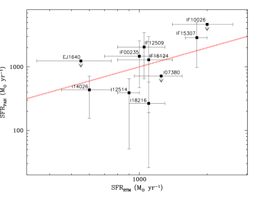
Figure 5: Comparison of the SFR estimated through PAH emission and through IR SED modelling using RTM (Farrah et al. 2002a; Rowan-Robinson 2000; Verma et al. 2002).

Figure 5 compares our SFR estimates with those obtained through modelling the IR SED using RTM (Rowan-Robinson 2000; Verma et al. 2002, F02). Both techniques seem to find consistent results. Despite most being AGN-dominated objects (see Sect. 5.2 below), we still found high star forming activity, with SFR $\sim 300-3000\leavevmode\nobreak\ M_{\mathrm{\sun}}\leavevmode\nobreak\ \mathrm{yr}^{-1}$ (see Table 3).

Figure 6 shows the SFR we calculated versus (a) total and (b) SB IR luminosity. We estimated the SB luminosity as:

$$L_{\mathrm{IR}}^{\mathrm{SB}}=(1-\alpha_{\mathrm{IR}})\leavevmode\nobreak\ L_{\mathrm{IR}},$$ (4)

where $\alpha_{\mathrm{IR}}$ is the fractional contribution of the AGN to the total IR luminosity (see Sect. 5.2) and $L_{\mathrm{IR}}$ is the total IR emission (8-1000 $\upmu$m) calculated through the IRAS fluxes (Sanders & Mirabel 1996). When only an upper limit is available for the IRAS fluxes at 12 or 25 $\upmu$m, we have simply assumed the one half of this limit. This convention provides a fair aproximation of the actual flux densities even for sources at moderate redshift (Nardini et al. 2009, 2010).

We performed several statistical tests to check any possible correlation between the SFR and the IR luminosities. Since our estimates of $L_{\mathrm{IR}}^{\mathrm{SB}}$ and SFR are both dependent of the parameter $\alpha_{6}$ (see Eqs. 2 and 7), we used a generalized Kendall’s Tau partial correlation test (Akritas & Siebert 1996). The result shows that both quantities are correlated with a probability $\sim 99.99\%>3\sigma$. This tight correlation between the star formation and SB IR luminosity is expected from several theoretical results (Kennicutt 1998; Draine & Li 2001, 2007, and references therein).

In the case of total IR luminosity versus SFR we can apply a generalized Kendall’s Tau test, since the estimate of the IR luminosity is completely independent of our estimate of the SFR. They show a weaker, but slightly significant, correlation (the probability is $98\%>2\sigma$). This slight correlation and the high SFR suggest that SB emission could be a significant contributor to the IR output (see Sect. 5.2).

5.2 AGN contribution to the IR luminosity

We define the 6 $\upmu$m-to-IR bolometric ratio as:

$$R=\dfrac{\nu_{6}f_{6}^{\mathrm{int}}}{F_{\mathrm{IR}}},$$ (5)

where $F_{\mathrm{IR}}$ is the total IR flux (8-1000 $\upmu$m) estimated as in Sanders & Mirabel (1996). The hypothesis that the IR and total bolometric fluxes are almost coincident is typically a fair assumption in ULIRG, but in principle we cannot adopt this hypothesis in our sources. The study of the HLIRG’s broad band SED has revealed that, for an important number of sources classified as HLIRG, a non-negligible fraction of the bolometric luminosity is emitted outside the IR range (Ruiz et al. 2010). Therefore we limited our analysis to the IR luminosity.

We can derive a connection between $R$ and the parameter $\alpha_{6}$:

$$R=\dfrac{R^{\mathrm{AGN}}\leavevmode\nobreak\ R^{\mathrm{SB}}}{\alpha_{6}\leavevmode\nobreak\ R^{\mathrm{SB}}+(1-\alpha_{6})\leavevmode\nobreak\ R^{\mathrm{AGN}}},$$ (6)

where $R^{\mathrm{AGN}}$ and $R^{\mathrm{SB}}$ are the equivalents of $R$ for pure (unobscured) AGN and pure SB, as defined in Eq. 5.

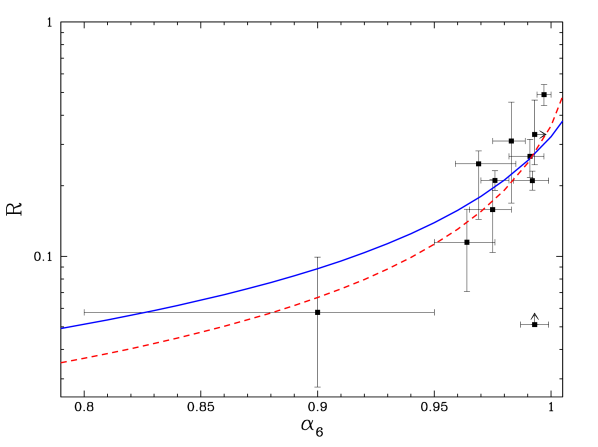
Figure 7: 6 $\upmu$m-to-IR ratio (R) versus $\alpha_{6}$. The red-dashed line is our best fit for the relation between R and $\alpha_{6}$ given by Eq. 6. The blue-solid line is the best fit obtained by N08 for a sample of ULIRG.

$R$ and $\alpha_{6}$ are both known quantities. Assuming $\alpha_{6}$ as the independent variable and $R$ as the dependent variable, we can fit Eq. 6 to the values observed in our sources, considering $R^{\mathrm{AGN}}$ and $R^{\mathrm{SB}}$ as free parameters. We found $R^{\mathrm{AGN}}=0.36\pm 0.08,R^{\mathrm{SB}}=\left(8\pm 3\right)\times 10^{-3}$. In spite of the limited size of our sample and the narrow range for $\alpha_{6}$, these results are in good agreement with those obtained by N08 for a larger sample of ULIRG: $R^{\mathrm{AGN}}=0.32^{+0.11}_{-0.08},R^{\mathrm{SB}}=\left(11.7^{+0.9}_{-0.7}\right)\times 10^{-3}$. Fig. 7 shows $R$ versus $\alpha_{6}$ for our sample of HLIRG, including our best-fit and the result from N08.

Using $\alpha_{6}$, $R^{\mathrm{AGN}}$ and $R^{\mathrm{SB}}$ (using the N08 values for the last two quantities), we could estimate the fractional AGN contribution ($\alpha_{\mathrm{IR}}$) to the IR output of each source:

$$\alpha_{\mathrm{IR}}=\dfrac{F_{\mathrm{IR}}^{\mathrm{AGN}}}{F_{\mathrm{IR}}}=\dfrac{\alpha_{6}}{\alpha_{6}+(R^{\mathrm{AGN}}/R^{\mathrm{SB}})(1-\alpha_{6})}.$$ (7)

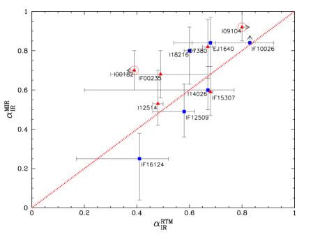
Figure 8: Comparison of the AGN contribution to the IR luminosity estimated through MIR spectral decomposition and through RTM. The blue squares are type I AGN and the red triangles are type II AGN and SB. The open circles mark those sources where our model is inaccurate. MIR contribution for IRAS 00182-7112 from Spoon et al. (2004a).

Figure 8 compares $\alpha_{\mathrm{IR}}$ estimated through our MIR spectral analysis and through the analysis of the IR SED using RTM (Rowan-Robinson 2000; Verma et al. 2002, F02;). Both estimates seem to be consistent in most sources. Letting aside those sources where our model is not suitable (IRAS 09104+4109 and IRAS 00182-7112), we found that the IR luminosity of seven out of ten HLIRG is AGN dominated. However, the SB contribution is also significant for all sources, spanning from $\sim 20\%-70\%$ (see Table 3). Using only the sources from the F02 sample, the mean SB contribution is $\sim 30\%$, close to $35\%$ obtained by F02. This significant SB contribution is consistent with the correlation we found between SFR and IR luminosity and the high SFR estimated (see Sect. 5.1). Our analysis confirms the idea that star formation and accretion into SMBH are both crucial phenomena to explain the properties of these extreme objects.

5.3 Covering Factor

An important physical parameter to unveil the distribution of dust in the nuclear environment of an AGN is the dust covering factor (CF), i.e. the fraction of sky covered by dust viewed from the central engine of the AGN. The CF is also critical to understand the fraction of direct nuclear emission that is absorbed by dust and re-emitted in the IR range and hence has a significant effect in the bolometric luminosity corrections of AGN.

The ratio between the thermal AGN luminosity (i.e., the IR reprocessed emission due to heated dust), $L^{\mathrm{AGN}}_{\mathrm{TH}}$, and the primary AGN luminosity (above $\sim 1$ $\upmu$m, i.e., the accretion disk bolometric emission), $L^{\mathrm{AGN}}_{\mathrm{BOL}}$, is commonly interpreted as an estimate of the dust CF (Maiolino et al. 2007; Rowan-Robinson et al. 2009; Roseboom et al. 2012):

$$\mathrm{CF(dust)}\approx\dfrac{L^{\mathrm{AGN}}_{\mathrm{TH}}}{L^{\mathrm{AGN}}_{\mathrm{BOL}}}.$$ (8)

The thermal AGN luminosity can be estimated through the MIR continuum emission. Assuming that the IR AGN luminosity is dominated by the dust emission and using the best-fit parameters obtained in our MIR spectral decomposition, the thermal emission is computed as:

$$L^{\mathrm{AGN}}_{\mathrm{TH}}\sim\dfrac{\alpha_{6}\leavevmode\nobreak\ \lambda\leavevmode\nobreak\ L_{\lambda}(6\leavevmode\nobreak\ \mu\mathrm{m})}{R^{\mathrm{AGN}}}.$$ (9)

X-ray emission is a primary product of the central engine of AGN, so X-ray luminosity is usually a good proxy to estimate the bolometric AGN luminosity (Maiolino et al. 2007; Rowan-Robinson et al. 2009). We applied the bolometric correction estimated by Marconi et al. (2004):

$$\log\dfrac{L^{\mathrm{AGN}}_{\mathrm{BOL}}}{L_{\mathrm{X}}}=1.54+0.24\mathcal{L}+0.012\mathcal{L}^{2}-0.0015\mathcal{L}^{3},$$ (10)

where $\mathcal{L}=\log\left(L^{\mathrm{AGN}}_{\mathrm{BOL}}/L_{\mathrm{\sun}}\right)-12$ and $L_{\mathrm{X}}$ is the intrinsic (i.e., absorption-corrected) 2-10 keV luminosity.

Therefore we can estimate the CF of those sources for which MIR and X-ray data are both available. Eight out of thirteen HLIRG in our sample fulfill this condition. The X-ray luminosities were obtained from Ruiz et al. 2007. IRAS F00235+1024 and IRAS 07380-2342 are probably Compton-Thick (CT) sources (Ruiz et al. 2007, 2010) so the upper limits on their X-ray luminosities have been increased by a factor of 60, the average ratio between intrinsic and observed X-ray luminosities in CT sources (Panessa et al. 2006). IRAS 14026+4341 was not detected in our X-ray analysis, but it has a counterpart in the 2XMMi catalogue (Watson et al. 2009). We estimated its 2-10 keV luminosity using the 2XMMi X-ray fluxes. Since this object seems to be an X-ray absorbed QSO (Ruiz et al. 2010), we applied the correction for CT objects described above to calculate its intrinsic X-ray luminosity.

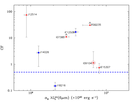
Figure 9: CF versus the AGN luminosity at 6 $\upmu$m. The blue dashed line is the estimated average CF for local QSO (see Sect. 5.3). Symbols as in Fig. 8.

Table 4 shows all the derived AGN luminosities and final estimates of the dust CF. The covering factors versus the AGN luminosities at 6 $\upmu$m are plotted in Fig. 9. For comparison, the plot includes the average CF estimated for local QSO.

Four out of eight objects show a dust CF consistent with $\sim 1$ (at 2$\sigma$ level) and sistematically above the average CF of local QSO ($\sim 0.5$). This result and the heavy X-ray absorption shown by most of these sources (all but one source, IRAS 14026+4341, show signatures of CT absorption in their X-ray emission, see Wilman et al. 2003; Iwasawa et al. 2005; Ruiz et al. 2007, 2010; Vignali et al. 2011) point towards large amounts of gas and dust enshrouding their nuclear environment as it has been found in local ULIRG (Spoon et al. 2004b; Verma et al. 2005; Yan et al. 2010).

We found one source with $\mathrm{CF}\sim 0.2$. This source, IRAS 18216+6418, is a QSO with no sign of X-ray or MIR obscuration. The low CF is consistent with previous studies finding a decrease in the CF of QSO with increasing luminosity (Maiolino et al. 2007; Treister et al. 2008). The decrease could be explained by “receding torus” models (Lawrence 1991; Maiolino et al. 2007; Hasinger 2008): low-luminosity AGN are surrounded by a dust torus of obscuring material covering a large fraction of the central source. High-luminosity AGN would be able to clean out the environment ionizing the surrounding medium or blowing it away through outflowing winds. Hence the opening angle of the torus would be larger and the covered solid angle would be lower (assuming the height of the torus is not luminosity-dependent).

The remaining three sources show $\mathrm{CF}>>1$. A dust CF above unity is usually interpreted as evidence of CT obscuration (Rowan-Robinson et al. 2009). As stated above, two objects (IRAS F00235+1024 and IRAS 07380-2342) were not detected in X-rays (Ruiz et al. 2007) and their broadband SED suggest that their low X-ray emission is due to high obscuration (Ruiz et al. 2010). Hence the bolometric AGN emission is probably underestimated in these sources. Observational and theoretical studies of CT AGN predict even larger values (i.e., $>>60$) for the intrinsic-to-observed X-ray luminosity ratio, depending on the amount of absorption and on the viewing angle with respect to the obscuring torus (Haardt et al. 1994; Iwasawa et al. 1997). The dust CF of these sources would be consistent with unity if the largest correction factor ($\sim 1000$) were applied.

The third remaining source, IRAS F12509+3122, is a QSO showing an X-ray emission significantly lower than the one predicted for a high-luminosity QSO, given its IR luminosity (Ruiz et al. 2010). This suggests that its bolometric AGN emission is also underestimated. However, the low X-ray luminosity of this object cannot be related to X-ray absorption (Ruiz et al. 2007). Alternatively, an increase with Eddington ratio has been observed in the X-ray bolometric correction of AGN ($\lambda_{Edd}=L_{BOL}/L_{Edd}$), from $\kappa_{X}\sim 15-30$ for $\lambda_{Edd}\lesssim 0.1$ to $\kappa_{X}\sim 70-120$ for $\lambda_{Edd}\gtrsim 0.2$ (Vasudevan & Fabian 2009). Using the SDSS optical spectrum of IRAS F12509+3122 and the McLure & Jarvis (2002) relation between black hole masses and MgII emission line widths, we estimated $\lambda_{Edd}\sim 0.5$ for this object. This high Eddington ratio suggests that the X-ray bolometric correction for this source could be higher than that obtained in Eq. 10. Further studies are needed to investigate how the Eddington ratio influences the X-ray luminosity of HLIRG.

6 Conclusions

We studied low resolution MIR spectra of thirteen HLIRG observed with Spitzer, nine of them also observed with XMM-Newton. We modelled their 5-8 $\upmu$m spectra, using the AGN/SB spectral decomposition technique developed by N08, and we estimated the contribution of each component to the total IR luminosity.

We found that all HLIRG in the sample harbour an AGN that clearly dominates the 5-8 $\upmu$m spectrum. Given the completeness of the F02 sample (nine out of ten F02 objects are included in our sample), this is strong evidence suggesting that all HLIRG harbour an AGN. We have also found that the AGN component seems to be the dominant power source of the total IR output in most sources. However, all sources, even the AGN-dominated HLIRG, show a significant SB activity, with a mean SB contribution of $\sim 30\%$. The SFR, estimated through the PAH emission, is also very high in all sources ($\sim 300-3000\leavevmode\nobreak\ M_{\mathrm{\sun}}\mathrm{yr}^{-1}$).

These results are in agreement with previous studies of HLIRG using theoretical models to reproduce their IR SED (F02; Rowan-Robinson 2000; Verma et al. 2002; Rowan-Robinson & Wang 2010), providing further support to the assumptions of these detailed models. The AGN relative contribution to the total IR output is also consistent with those estimated through SED modeling. The large mean AGN contribution we found ($\sim 70\%$) is consistent with previous studies of ULIRG, pointing towards an increase of the AGN emission with increasing luminosity (Veilleux et al. 2002; Nardini et al. 2010). Our work confirms the crucial role of both AGN and SB phenomena to explain the properties of these extreme sources.

Using X-ray and MIR data we were able to estimate the covering factor (CF) of these HLIRG, finding that a significant fraction (seven out of eight) have CF$\gtrsim 1$. Most of these sources with large CF also show heavy X-ray absorption and high optical depth or absorption features in their MIR spectrum. This strongly suggests that the nuclear environment of these sources is heavily enshrouded by large amounts of gas and dust, as it has been observed in local ULIRG.

F02 proposed that HLIRG could be divided in two populations: (1) mergers between gas-rich galaxies, as found in the ULIRG population, and (2) young active galaxies going through their maximal star formation periods whilst harbouring an AGN. In Ruiz et al. (2010) we found strong evidence supporting the two-population hypothesis. Han & Han (2012) studied the same HLIRG sample using AGN and SB theoretical models and bayesian techniques to fit their IR SED. They found further evidence that the physical properties of AGN and SB harboured by HLIRG could be divided into two populations: SB-dominated HLIRG (corresponding to our “ULIRG-like” objects) show a higher fraction of OB stars and the starburst region is more compact, while AGN-dominated objects show a dustier thorus. Additional evidence favouring this two-populations idea is presented by Draper & Ballantyne (2012). They suggest, based on recent Herschel observations, that major mergers cannot explain the total population of luminous high-$z$ ULIRG harbouring AGN.

All sources showing $\mathrm{CF}\sim 1$ (except IRAS 14026+4341) were classified as “ULIRG-like” objects in Ruiz et al. (2010) while IRAS 18216+6418, with a significantly lower CF, was classified as a “non-ULIRG” source. Furthermore, IRAS F00235+1024 and IRAS F15307+3252, both sources showing a high CF, were observed by the Hubble Space Telescope (HST) and both present signs of recent mergers. On the other hand, IRAS 18216+6418, also observed by HST, shows no signs of interactions or mergers (Farrah et al. 2002b). The study of the dust CF adds another piece of evidence favouring that HLIRG can be separated into two differentiated populations, although further studies with larger samples of HLIRG are needed to obtain stronger conclusions.

Table 1: Spitzer observations of HLIRG.

Sources	Sample	Type	R.A.	DEC.	$z$	AOR	Exposure (s)	Date
IRAS 00182-7112	X	QSO2	00 20 34.7	-70 55 27	0.327	7556352	94.4	2003-11-14
IRAS F00235+1024†	F, X	NL-SB	00 26 06.5	+10 41 32	0.575	12237056	94.4	2005-08-11
IRAS 07380-2342†	F, X	NL	07 40 09.8	-23 49 58	0.292	12236032	12.6	2005-03-23
IRAS 09104+4109	X	QSO2	09 13 45.4	+40 56 28	0.442	6619136	73.4	2003-11-29
IRAS F10026+4949	F	Sy1	10 05 52.9	+49 34 42	1.120	4738560	14.7	2004-04-17
IRAS F12509+3122	F, X	QSO	12 53 17.6	+31 05 50	0.780	12236800	62.9	2005-06-06
IRAS 12514+1027	X	Sy2	12 54 00.8	+10 11 12	0.32	4978432	94.4	2005-02-06
IRAS 14026+4341†	F, X	QSO	14 04 38.8	+43 27 07	0.323	4374016	102.8	2005-05-22
IRAS F15307+3252	X	QSO2	15 32 44.0	+32 42 47	0.926	4983552	243.8	2004-03-04
IRAS F16124+3241	F	NL	16 14 22.1	+32 34 04	0.71	4984832	243.8	2005-03-19
ELAIS J1640+41	F	QSO	16 40 10.1	+41 05 22	1.099	11345664	243.8	2005-08-13
IRAS 18216+6418	F, X	QSO	18 21 57.3	+64 20 36	0.297	4676096	31.5	2004-04-17
IRAS F23569-0341	F	NL	23 59 33.6	-03 25 13	0.59	12235776	243.8	2004-12-13

Notes.

Table 2: Best-fit model parameters (c.f. Sect. 4).

Sources	Model	$\chi^{2}/$d.o.f.	$f_{6}^{\mathrm{int}}$ (mJy)	$\alpha_{6}$	Spectral index	$\tau_{6}$	Additional features
IRAS F00235+1024	A	238 / 75	$\mathbf{86\pm 5}$	$\mathbf{0.982\pm 0.002}$	$\mathbf{0.8}$	$\mathbf{2.57\pm 0.06}$	…
	B	218 / 74	$46^{+32}_{-2}$	$0.969^{+0.012}_{-0.003}$	$>1.0$	$1.93^{+0.53}_{-0.05}$	…
IRAS 07380-2342	A	22 / 76	$\mathbf{213\pm 12}$	$\mathbf{0.988\pm 0.006}$	$\mathbf{0.8}$	$\mathbf{0.49\pm 0.05}$	…
	B	16 / 75	$130^{+43}_{-1}$	$0.990\pm 0.009$	$1.64^{+0.03}_{-0.48}$	$<0.3$	…
IRAS 09104+4109*	A	44 / 69	$\mathbf{176\pm 3}$	$\mathbf{0.995\pm 0.002}$	$\mathbf{0.8}$	$\mathbf{0.69\pm 0.02}$	[NeVI] emission line
	B	26 / 68	$104\pm 11$	$0.996\pm 0.004$	$1.65\pm 0.17$	$0.16\pm 0.10$	[NeVI] emission line
IRAS F10026+4949	A	19 / 88	$\mathbf{149^{+8}_{-18}}$	$\mathbf{>0.988}$	$\mathbf{0.8}$	$\mathbf{0.63^{+0.06}_{-0.12}}$	…
	B	19 / 87	$150\pm 60$	$>0.992$	$0.7^{+0.7}_{-0.5}$	$0.6^{+0.3}_{-0.5}$	…
IRAS F12509+3122	A	51 / 85	$\mathbf{25.3^{+0.8}_{-0.3}}$	$\mathbf{0.959^{+0.005}_{-0.003}}$	$\mathbf{0.8}$	$\mathbf{<0.04}$	…
	B	51 / 84	$25\pm 6$	$0.962^{+0.008}_{-0.003}$	$0.87^{+0.02}_{-0.41}$	$<0.2$	…
IRAS 12514+1027	A	116 / 73	$\mathbf{57.4\pm 1.0}$	$\mathbf{0.958\pm 0.003}$	$\mathbf{0.8}$	$\mathbf{<0.02}$	[NeVI] emission line
	B	114 / 72	$57\pm 7$	$0.956\pm 0.004$	$0.77^{+0.01}_{-0.22}$	$<0.12$	[NeVI] emission line
IRAS 14026+4341	A	33 / 75	$\mathbf{75\pm 2}$	$\mathbf{0.977\pm 0.004}$	$\mathbf{0.8}$	$\mathbf{0.06\pm 0.02}$	…
	B	31 / 74	$70^{+13}_{-1}$	$0.978\pm 0.004$	$0.93^{+0.02}_{-0.31}$	$<0.18$	…
IRAS F15307+3252	A	238 / 84	$\mathbf{38\pm 2}$	$\mathbf{0.981\pm 0.004}$	$\mathbf{0.8}$	$\mathbf{0.64\pm 0.04}$	…
	B	173 / 83	$21^{+6}_{-1}$	$0.975\pm 0.006$	$>1.4$	$0.07^{+0.24}_{-0.03}$	…
IRAS F16124+3241	A	38 / 78	$\mathbf{6.6\pm 1.3}$	$\mathbf{0.87^{+0.03}_{-0.04}}$	$\mathbf{0.8}$	$\mathbf{1.3\pm 0.2}$	…
	B	38 / 77	$7\pm 4$	$0.87^{+0.05}_{-0.11}$	$0.8^{+1.0}_{-0.6}$	$1.3^{+0.5}_{-0.8}$	…
ELAIS J1640+41	A	33 / 88	$\mathbf{17.3\pm 1.1}$	$\mathbf{0.993\pm 0.006}$	$\mathbf{0.8}$	$\mathbf{0.13\pm 0.06}$	…
	B	32 / 87	$15^{+6}_{-1}$	$>0.988$	$1.06^{+0.02}_{-0.60}$	$<0.4$	…
IRAS 18216+6418	A	117 / 77	$136.1^{+2.2}_{-0.4}$	$>0.999$	$0.8$	$<0.001$	…
	A	18 / 76	$\mathbf{159^{+7}_{-19}}$	$\mathbf{0.991^{+0.005}_{-0.003}}$	$\mathbf{<0.4}$	$\mathbf{<0.17}$	…

Notes.

Table 3: SFR and AGN relative contributions to the IR output, and IR luminosities (in cgs units).

Sources	SFR	$\alpha_{\mathrm{IR}}$	$L_{\mathrm{IR}}$	$L_{\mathrm{IR}}^{\mathrm{SB}}$
	[$M_{\mathrm{\sun}}\mathrm{yr^{-1}}$]		[$\times 10^{46}$]	[$\times 10^{46}$]
IRAS F00235+1024	$1500^{+1100}_{-1000}$	$0.68\pm 0.12$	$20\pm 8$	$6\pm 4$
IRAS 07380-2342	$<700$	$0.82^{+0.14}_{-0.16}$	$14.2\pm 0.6$	$3\pm 2$
IRAS 09104+4109*	$<600$	$0.92^{+0.08}_{-0.07}$	$13.8\pm 1.3$	$1.1^{+1.1}_{-0.9}$
IRAS F10026+4949	$<500$	$>0.8$	$140\pm 40$	$<20$
IRAS F12509+3122	$2000\pm 1400$	$0.49^{+0.14}_{-0.13}$	$36\pm 13$	$18\pm 8$
IRAS 12514+1027	$400\pm 300$	$0.53^{+0.17}_{-0.11}$	$3.7\pm 0.4$	$1.7^{+0.7}_{-0.5}$
IRAS 14026+4341	$400\pm 300$	$0.60^{+0.12}_{-0.10}$	$6.2\pm 0.5$	$2.5^{+0.8}_{-0.7}$
IRAS F15307+3252	$3000\pm 2000$	$0.59^{+0.13}_{-0.12}$	$52\pm 17$	$21^{+10}_{-9}$
IRAS F16124+3241	$1300^{+1700}_{-1100}$	$0.25^{+0.13}_{-0.21}$	$16\pm 6$	$12^{+5}_{-6}$
ELAIS J1640+41	$<1200$	$0.82^{+0.13}_{-0.11}$	$<120$	$<20$
IRAS 18216+6418	$300^{+300}_{-200}$	$0.80^{+0.12}_{-0.17}$	$8.0\pm 1.4$	$1.6^{+1.0}_{-1.4}$

Notes.

Table 4: AGN luminosities (in cgs units) and CF values.

Sources	$L_{\mathrm{X}}$	$L_{\mathrm{AGN}}^{\mathrm{DIR}}$	$\lambda\leavevmode\nobreak\ L_{\lambda}(6\leavevmode\nobreak\ \mu\mathrm{m})$	$L_{\mathrm{AGN}}^{\mathrm{TH}}$	CF
	[$\times 10^{44}$]	[$\times 10^{46}$]	[$\times 10^{46}$]	[$\times 10^{46}$]
IRAS F00235+1024†	$<1.6$	$<0.6$	$6.1\pm 1.2$	$19^{+8}_{-6}$	$>30$
IRAS 07380-2342†	$<2.0$	$<0.8$	$3.0\pm 0.3$	$9^{+3}_{-2}$	$>11$
IRAS 09104+4109	$20^{+26}_{-4}$	$19^{+31}_{-4}$	$6.8\pm 0.3$	$21^{+7}_{-5}$	$1.1^{+1.9}_{-0.4}$
IRAS F12509+3122	$1.8\pm 0.2$	$0.73\pm 0.09$	$3.9\pm 0.3$	$12^{+4}_{-3}$	$16^{+6}_{-5}$
IRAS 12514+1027	$0.2^{+4.5}_{-0.1}$	$0.04^{+1.41}_{-0.03}$	$0.88\pm 0.06$	$2.7^{+1.0}_{-0.7}$	$70^{+3000}_{-60}$
IRAS 14026+4341†	$3.0\pm 1.8$	$1.4^{+1.0}_{-0.9}$	$1.27\pm 0.07$	$4.0^{+1.4}_{-1.0}$	$2.8^{+2.2}_{-1.9}$
IRAS F15307+3252	$31^{+7}_{-8}$	$34^{+9}_{-10}$	$8.1\pm 0.7$	$25^{+9}_{-7}$	$0.7\pm 0.3$
IRAS 18216+6418	$37\pm 4$	$43\pm 5$	$2.11\pm 0.10$	$6.6^{+2.3}_{-1.7}$	$0.15^{+0.06}_{-0.04}$

Notes.

Figure 6: SFR estimated using the PAH emission at 7.7 $\upmu$m versus (a) total and (b) starburst IR luminosities. The open circles mark those sources where our model is inaccurate.