On the Role of Rotating Sunspots in the Activity of Solar Active Region NOAA 11158

Abstract

We study the role of rotating sunspots in relation to the evolution of various physical parameters characterizing the non-potentiality of the active region NOAA 11158 and its eruptive events using the magnetic field data from the Helioseismic and Magnetic Imager (HMI) and multi-wavelength observations from the Atmospheric Imaging Assembly (AIA) on board Solar Dynamics Observatory (SDO). From the evolutionary study of HMI intensity and AIA channels, it is observed that the AR consists of two major rotating sunspots one connected to flare-prone region and another with CME. The constructed space-time intensity maps reveal that the sunspots exhibited peak rotation rates coinciding with the occurrence of the major eruptive events. Further, temporal profiles of twist parameters, viz., average shear angle, $\alpha_{\rm av}$, $\alpha_{\rm best}$, derived from HMI vector magnetograms and the rate of helicity injection, obtained from the horizontal flux motions of HMI line-of-sight magnetograms, corresponded well with the rotational profile of the sunspot in CME-prone region, giving predominant evidence of rotational motion to cause magnetic non-potentiality. Moreover, mean value of free-energy from the Virial theorem calculated at the photospheric level shows clear step down decrease at the on set time of the flares revealing unambiguous evidence of energy release, intermittently that is stored by flux emergence and/or motions in pre-flare phases. Additionally, distribution of helicity injection is homogeneous in CME prone region while it is not and often changes sign in flare-prone region. This study provides clear picture that both proper and rotational motions of the observed fluxes played significant role to enhance the magnetic non-potentiality of the AR by injecting helicity, twisting the magnetic fields thereby increasing the free energy, leading to favorable conditions for the observed transient activity.

1 Introduction

Activity level of the Sun is defined by eruptive events like coronal mass ejections (CMEs) and flares occurring in the ARs consisting of groups of sunspots having positive and negative magnetic polarities. During the evolution of ARs, the sunspots exhibit motions, both proper and rotational, that lead to the storage of energy in the AR by increasing its magnetic non-potentiality. The eventual release of stored energy then occurs in the form of the eruptive events, such as, flares and CMEs. An investigation of the characteristics of sunspots can thus help towards the understanding of transient solar activities.

Rotational motions of and around sunspots have been observed by several authors in the past (Evershed, 1910; Bhatnagar, 1967; McIntosh, 1981). More recent studies have also reported sunspot rotations about umbral center as well as about another sunspot with the availability of high spatial and temporal resolution data from space borne as well as ground based observatories (Brown et al., 2003; Zhang et al., 2007; Yan et al., 2009). Rotational motions can shear and twist the overlying magnetic field structures thereby storing excess energy. Vertical current, current helicity and transport helicity are some of the quantitative parameters derived from observations that are related to the twisting of fieldlines anchored in the moving footpoints. CMEs that disturb the space environment are thought to occur due to an over-accumulation of helicity and its ejection from the corona to the interplanetary space. Recently, Zhang et al. (2008) reported that helicity injection as inferred from the rotational motion of sunspots can be comparable to that as deduced for the entire AR by local correlation tracking (LCT) method. They also found good spatial and temporal correlation of sunspot rotational motion with two homologous flares.

The consequences of sunspot rotations and related changes, both in photosphere and corona, have been investigated by several workers. Relationships between the sunspot rotation and coronal consequences (Brown et al., 2003; Tian & Alexander, 2006; Tian et al., 2008), flare productivity (Yan et al., 2008; Zhang et al., 2008), statistics of the direction of rotating sunspots, helicities (Yan et al., 2008, and references there in), and the association of flares with abnormal rotation rates (Hiremath et al., 2005) are some studies in this direction.

In this study, we report on the rotating sunspots observed during February 11-16, 2011, in AR NOAA 11158. We present the results related to the changes in various parameters, viz., vertical current, twist parameters, helicity injection, and the free energy of the AR during its evolution. Further, we examine whether the rotating sunspots were associated to the eruptive flare and CME events of the AR. Our aim is towards finding association of the observed uncommon rotation of the sunspots of this AR in terms of changes in various physical parameters. We have organized the paper as follows: Observational data and analysis procedure is described in Section 2 which is followed by the results with possible discussion in Section 3. Finally, the summary of the study is presented in Section 4.

2 Observational Data and Analysis Procedure

The observational data used in this study are obtained from the Helioseismic and Magnetic Imager (HMI; Schou et al. 2012) and the Atmospheric Imaging Assembly (AIA, Lemen et al. 2012) on board Solar Dynamics Observatory (SDO).

AIA observes the sun in ten different wavelengths in soft X-ray, EUV and UV regimes to study the processes occurring at various atmospheric layers i.e., chromosphere, transition region and corona, at a pixel size of 0.6″ and 12 second cadence. In addition, we also obtained high resolution G-band 4300Å and Ca ii H 3970Å images from Solar Optical Telescope (SOT; Tsuneta et al. 2008) on board Hinode for understanding the associated chromospheric structures. Data on the CME and flare initiation times were obtained from the websites, .

HMI observes the full solar disk in the Fe i 6173Å  spectral line with a spatial resolution of 0.5″ /pixel and provides four main types of data at a cadence of 12 minutes: dopplergrams (maps of solar surface velocity), continuum filtergrams (broad-wavelength maps of the solar photosphere), and both line-of-sight (LOS) and vector magnetograms. Filtergrams are obtained at six wavelength positions centered at the Fe i line to compute Stokes parameters I, Q, U, V. These are then reduced with the HMI science data processing pipeline to retrieve the vector magnetic field using the Very Fast Inversion of the Stokes Vector algorithm (VFISV; Borrero et al. 2011) based on the Milne-Eddington atmospheric model. The inherent 180°  azimuthal ambiguity is resolved using the minimum energy method (Metcalf, 1994; Leka et al., 2009). Data processing is carried out by the HMI vector team (Hoeksema & et al., 2012) and the products are made available to the solar community.

We used the high resolution continuum images of NOAA 11158 obtained from the HMI for the rotation measurement of sunspots. In order to estimate the twisting in various sites of the AR, we used vector magnetograms projected and remapped to heliographic coordinates. The intensity images obtained from AIA were used to examine the coronal changes associated to the photospheric motions. All images both from AIA and HMI taken at different times were aligned by differentially rotating to an image at central meridian by non-linear remapping method (Howard et al., 1990). For our analysis, we have used the standard SolarSoft routines (SSW; Freeland & Handy 1998) implemented in Interactive Data Language(IDL).

In order to further characterize the association of rotational motion on non-potentiality and in turn on the observed transient activity of the AR, we examine the evolution of magnetic fluxes and the derived parameters (see Leka & Barnes (2003) for definitions of various non-potential parameters) therefrom. We evaluate the vertical currents and shear or twist parameters to estimate the extent of non-potentiality. The complexity developed through the flux motions by helicity injection rate and consequent magnetic energy storage are also analyzed. Procedures for these calculations are briefly outlined below:

1. We evaluate the total absolute flux in sub-regions R1 and R2 by summing over all the pixels $F=\sum|B_{z}|$. The vertical current is computed from the Ampere’s law $\nabla\times\bf{B}=\mu_{0}\bf{J}$, where the permeability of free space $\mu_{0}=4\pi\times 10^{-7}$ Henry/meter. Using the z-component of this relation, one can deduce the total absolute vertical current as $J_{z}=\sum|(\nabla\times\mathbf{B})_{z}/\mu_{0}|$.

2. Magnetic Shear: Non-potential nature of magnetic field is characterized by magnetic shear defined as difference between directions of observed transverse field and potential transverse field (Ambastha et al., 1993; Wang et al., 1994) and is given by

   $$S=B\cdot\theta=B\cdot\left(\cos^{-1}\frac{\mathbf{B}\cdot\mathbf{B_{p}}}{BB_{p}}\right)$$ (1)

   where $B=|\mathbf{B}|$ is magnitude of observed magnetic field and $B_{p}=|\mathbf{B_{p}}|$ is magnitude of potential field computed from fourier method (Gary, 1989). The weighted shear angle in a region of interest with N pixels can then be obtained as

   $${\rm WSA}=\frac{\sum_{i}^{N}S_{i}}{\sum_{i}^{N}B_{i}}$$ (2)

   and will estimate the overall angle of departure from potential field configuration.

3. Alpha best ($\alpha_{\rm best}$): The force free parameter $\alpha_{\rm best}$ is used as a proxy to monitor the extent of twist of the magnetic fieldlines in an AR. For this parameter, the extrapolated force free fields best fit the observed transverse fields in the sense of a minimum least-squared difference on the photosphere. The procedure of the fitting method for calculating $\alpha_{\rm best}$ (Pevtsov et al., 1994; Hagino & Sakurai, 2004) is as follows. For a given $\alpha$ and with observed $B_{z}$, we compute linear-force free field whose transverse component is $B_{t,cal}$. We then search for the $\alpha$ that gives minimum residual ($R(\alpha)$) of transverse component in a range of values through the following equation

   $$R{\alpha}=\frac{\sum[B_{t,obs}(x,y)-fB_{t,cal}(x,y,\alpha)]^{2}}{\sum B^{2}_{\rm t,obs}}$$ (3)

   $${\rm where}\hskip 14.45377ptf=\frac{\sum B^{2}_{\rm t,obs}}{\sum B^{2}_{\rm t,cal}(x,y)}\$$ (4)

   The error in the fitting of residual and $\alpha$ that is effected in estimating $\alpha_{\rm best}$ is given by

   $$\delta\alpha^{2}_{best}=\frac{2\delta B_{t}\sqrt{R_{0}}}{R^{\prime}\sqrt{\sum B^{2}_{\rm t,obs}}}$$ (5)

4. Average Alpha ($\alpha_{\rm av}$): Another proxy for representing the twist is obtained by taking the average of $\alpha$ from the force-free assumption of photospheric fields, i.e., $\nabla\times\textbf{B}=\alpha\textbf{B}$. Following Pevtsov et al. (1994) and Hagino & Sakurai (2004), it is given by:

   $$\alpha_{\rm av}=\frac{\sum J_{z}(x,y){\rm sign}[B_{z}(x,y)]}{\sum|B_{z}|}$$ (6)

   The error in $\alpha_{\rm av}$ is deduced from the least squared regression in the plot of $B_{z}$ and $J_{z}$, and is given by:

   $$\delta\alpha_{\rm av}^{2}=\frac{\sum[J_{z}(x,y)-\alpha_{\rm av}B_{z}(x,y)]^{2}/|B_{z}(x,y)|}{(N-1)\sum|B_{z}(x,y)|}$$ (7)

   where N is the number of pixels where $|B_{t}|\geq 150$G (with 150G assumed as the lower cut-off for the transverse field.)

5. Helicity Injection: One uses the helicity injection rate to quantify the twist due to photospheric flux motions. Following Pariat et al. (2005):

   $$\frac{dH}{dt}=\frac{-1}{2\pi}\int_{S}\int_{S^{\prime}}\frac{[(\textbf{x}-\textbf{x}^{\prime})\times(\textbf{u}-\textbf{u}^{\prime})]_{n}}{|\textbf{x}-\textbf{x}^{\prime}|^{2}}B^{\prime}_{n}(\textbf{x}^{\prime})B_{n}(\bf{x})dS^{\prime}dS\\$$ (8)

   where $\textbf{u}(\textbf{u}^{\prime})$ is the foot-point velocity at position vector $\bf{x}(\bf{x}^{\prime})$, and $B_{n}$ is the normal component of magnetic field from observations. This equation shows that the helicity injection rate can be understood as the summation of rotation rates of all the pairs of elementary fluxes weighted with their magnetic flux. Integration of above equation in the observed time interval provides the accumulated helicity, $\Delta H=\int(dH/dt)\Delta{t}$ that is injected due to foot-point shear motions.

6. Magnetic Free Energy: One can get the estimate of non-potentiality by the magnetic virial theorem (Chandrasekhar, 1961; Molodensky, 1974; Low, 1982), which gives the total force-free magnetic energy as

   $$E_{m}=\int_{z>0}\frac{\bf{B}^{2}}{8\pi}dV=\frac{1}{4\pi}\int_{z=0}(xB_{x}+yB_{y})B_{z}dxdy$$ (9)

   where $B_{x}$, $B_{y}$ are the horizontal and $B_{z}$ the vertical components of magnetic field $\bf B$ at position (x, y) on the solar surface z=0. The applicability of this equation to the realistic situations like solar photospheric boundary must be restricted by force-freeness of the field and flux balance conditions. Despite its applicability, it should have some useful information about energy storage and release. Since the potential field state is a minimum energy state, by subtracting the potential field energy from the force-free energy one gets the upper limit of the free-energy available in the AR to account for the flares and CMEs.

   However, the photospheric field is not strictly force-free (Metcalf et al., 1995; Gary, 2001) and flux balance in the region of interest are not fully satisfied. Therefore, one obtains incorrect estimates of the free-energy. To derive the error estimate for the force-free energy measurement, we have adopted the Pseudo-Monte Carlo method (Metcalf et al., 2005), which gives the mean and variance of energy estimate by changing the origin of coordinate system in all possible ways. It includes both the statistical error as well as the error due to the departure from the force-free state of the fields.

We have examined the errors given with the vector field data after inversion of stokes profiles. The maximum error in transverse field $B_{t}$ in the entire data set varied in the range of 20-35G. The total field strength was observed to vary by 50G over a day due to various factors (Hoeksema & et al., 2012). Therefore, we carried out the calculations with $|B_{t}|\geq 150$G and $|B_{z}|\geq 15$G and neglected the pixels having magnetic fields below these thresholds, simultaneously.

As require by Equation 8, the horizontal motions of photospheric fluxes using LOS magnetic field data obtained at a cadence of 12 minutes by the method of Affine Velocity Estimator (DAVE; Schuck 2006). It is a local optical flow method that determines the mass velocities within the windowed region. Further, it adopts an affine velocity profile specifying velocity field in the windowed region about a point and constrains that profile to satisfy the induction equation. The maximum rms velocities of flux motions in the entire AR were found to be distributed in the range 0.6-0.9 kms^-1. These velocity maps of mass motions revealed strong shear flows that included both proper and rotational motions. With the velocities of these flux motions, we computed the helicity flux density maps of the whole AR at pixels above 10G to reduce computation time, then helicity injection rate, and accumulated helicity using Equation 8.

3 Results and Discussion

The AR NOAA 11158 was a newly emerging region that first appeared as small pores on the solar disk on February 11, 2011 at the heliographic location E33S19. Subsequently it grew rapidly by merging of small pores to form bigger sunspots and developed to $\beta\gamma\delta-$ magnetic complexity on 2011 February 13. The HMI intensity maps in Figure 1 show the spatio-temporal evolution of AR 11158 during 2011 February 11-16. The prominent negative and positive polarity sunspots are labeled in frame (d) as SN1–SN3, SP1–SP3, respectively, along with the overlaid LOS magnetic field contours in frame (e) depicting the polarity distribution of the AR. The overall configuration of the AR is seen to be of quadrupolar nature. The proper motion of individual sunspots during February 13–16 are marked by arrowed curves traced by centroids of the sunspots as shown in frame (f).

In what follows, we shall present evolution of the AR during 2011 February 13-15 using coronal observations in different wavelengths along with the changes in its magnetic and velocity field structures, the related physical parameters and the flare/CME activities.

3.1 Evolution and the Activity of the AR

A careful examination of the animations of magnetogram and intensity maps revealed significant counter clock-wise (CCW) rotation of SN1 and clock-wise (CW) rotation of SP2 during February 13-15. We selected two sub-regions based on distinctive flux motions and associated transient activities. These are sub-region R1 covering SN1, and R2 around SN2, SN3, and SP2 as shown in the rectangular boxes in Figure 1(d).

The spatial evolution in R2 displayed a large shearing motion of SP2 that itself rotated clock-wise during February 13-15. It then detached from SN2 and moved towards SP3 with small patches of both polarities appearing and disappearing over short periods of time.In R1, a small positive polarity site SP1 emerged to the north of SN1 that rotated in a similar counter-clockwise direction along with a proper motion away from SN1. The rotation of SN1 and its associated SP1 twisted the field lines. These motions appears to have resulted in a large magnetic non-potentiality in this sub-region. This followed the first X-class event of the current solar cycle 24, an X2.2 flare in R2 on February 15. In addition, several flares of smaller magnitude, including four M-class and several C-class occurred during this period; all associated to R2 except the M2.2 flare of 14 February which is observed to originate from R1. Many intermittent CMEs were also launched from this AR. These flares and CMEs (listed in Table 1) appear to be related to the observed motions in the AR. We have manually traced the the QuickLook AIA images to look for mass ejections in 304Å channel locating the sub-region they belonged to and found that most of the CMEs originated from R1 (except the one associated with the X2.2 flare from R2). This inference is further confirmed by the STEREO space-craft information.

Table 1: List of Flares and CMEs

AR	Date	Flares	CMEs
(NOAA)	dd/mm/yyyy	magnitude(time UT)	(time UT)
11158	13/02/2011	C1.1(12:36),C4.7(13:44),M6.6(17:28)	21:30,23:30
	14/02/2011	C1.6(02:35),C8.3(04:29),C6.6(06:51)	02:40,07:00,12:50
		C1.8(08:38),C1.7(11:51),C9.4(12:41)	17:30,19:20
		C7.0(13:47),M2.2(17:20),C6.6(19:23)
		C1.2(23:14),C2.7(23:40)
	15/02/2011	C2.7(00:31),X2.2(01:44),C4.8(04:27)	00:40,02:00,03:00
		C1.0(10:02),C4.8(14:32),C1.7(18:07)	04:30,05:00,09:00
		C6.6(19:30),C1.3(22:49)

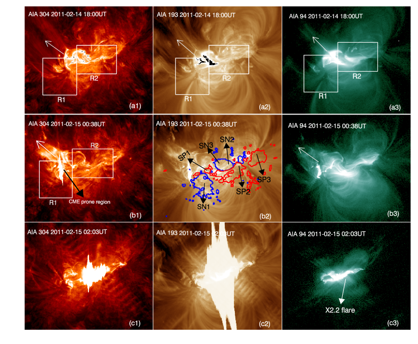
Figure 2: The coronal activity observed during the evolution of the AR in AIA  wavelengths. (a1–a3): A mass expulsion (dashed arrow) from R1 which eventually turned to a CME on 2011 Feb 14/18:00UT. (b1–b3): Another mass expulsion observed on 2011 Feb 15/00:36 UT from the same location. (c1): Bright emission seen during the X2.2 flare, saturating the 193Å detector (c2) and the twisted flux ropes along the polarity inversion line as seen in 94Å  (c3).

Morphological changes observed in chromosphere, transition region, and coronal regions corresponding to some of the transient events are shown in Figure 2 using AIA observations in 304, 193 and 94Å wavelengths. We further examine the characteristics of non-potentiality in the selected sub-regions.

Figure 2 (a1–a3) shows a large mass expulsion from sub-region R1 that turned into a large CME on February 14/18:00UT with the associated flare M2.2 at 17:20UT. It appeared to occur when the rotation of SN1 had attained the maximum speed. This CME began at 17:30UT and continued well past 19:30UT as observed from the AIA/304Å movies. The ejected plasma (marked by arrow in a1) is visible in 304Å as it is sensitive to the chromospheric temperature ($\approx 10^{4}$K). However, it is only partially visible in 193Å and not discernible in 94Å except for the cusp shaped fieldlines filled with the hot bright plasma at $\sim 10^{6}$K. Another such mass ejection of February 15/00:36UT that ensued from the same location is shown in Figure 2(b1–b3). The LOS magnetic field contours are overlaid in frame b2 for reference, depicting the fieldline connectivities from the magnetic footpoints in the labeled sunspots. From the animations of magnetic and intensity images and coronal fieldline connectivity, a significant role of new emerging flux at SP1 can be inferred in these expulsions.

Figure 2 (c1–c3) shows the intense X2.2 flare which occurred on February 15 in sub-region R2. This event was also associated with a halo-CME which began at 01:44UT. This flare produced abnormal magnetic polarity reversal and Doppler velocity enhancement during the flare’s impulsive phase (Maurya et al., 2012). As mentioned earlier, the rotating flux footpoints, i.e., the sunspots, twisted the overlying magnetic structures in opposite directions. The rotational motion of the positive polarity spot SP2 about its negative polarity counterpart SN2 developed strongly twisted fieldlines along the polarity inversion line (PIL), clearly visible as a “sigmoidal” structure (c3). As reported earlier, such sigmoidal magnetic field structures are more likely to erupt (Canfield et al., 1999).

3.2 Measurement of Sunspot Rotation

To derive the rotational parameters of the sunspots, we followed the procedure as explained in Brown et al. (2003). Essentially, we pursued the motion of a distinct feature in the penumbra as it is comparatively richer than the umbra. We uncurl the annular region of penumbra by transforming from the Cartesian (x–y) frame to the polar (r-$\theta$) plane. In this way, we can measure the position angle of the observed feature as displaced from its previous position as the sunspot rotated. We identified the centroid of the sunspot SN1 by setting the 50% contrast between the umbra and penumbra in the time sequence of intensity images around the region of a circular disk of radius 18 arc-sec. This circular region was then remapped on to the polar coordinate system from the Cartesian, so that annular features appeared as straight strips from umbra to penumbra. Once this is done, any portion of the strip could be tracked in time to determine the angular distance by which a particular feature is displaced.

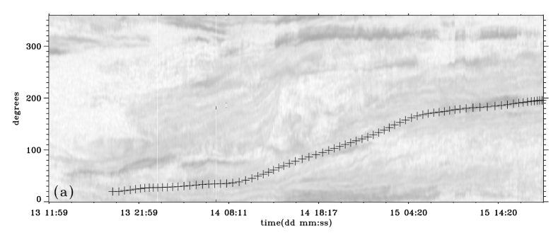
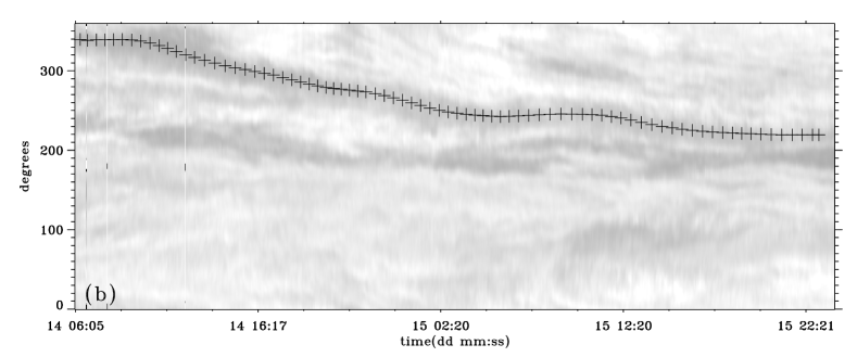
Figure 3: Space-time map of a strip in (a) the sunspot SN1 (at a distance of 7 arc-sec from the sunspot’s centroid), (b) sunspot SP2 (at a distance of 11 arc-sec from the sunspot’s centroid), after remapping the annular region of the sunspot to the r-$\theta$ plane. Rotation angle ($\theta$) and rotation rate ($d\theta/dt$) of the sunspot’s umbrae are inferred from the well-appearing diagonal feature in (a)-(b) sampled along the path marked by “+”, and plotted with time in (c)-(d), respectively.

We constructed the space-time diagrams for both the rotating sunspots, SN1 and SP2, extracted at the radii of 11″ and 7″ from their umbral centroid, as shown in Fiugre 3(a-b), respectively. Rotational motion of the features in the penumbral regions can be seen as diagonal bright or dark streaks. The uncurling starts at westward point chord connecting the centroid position and the outer circle of annular portion and proceeds anti-clockwise about the sunspot centroid. These diagrams clearly show the counter-clock wise (CCW) rotation of SN1 in sub-region R1, and the clock wise (CW) rotation of SP2 in sub-region R2. A well observed streak is traced and plotted as marked by “+” at the respective positions as angular displacement ($\theta$) and its time derivative i.e., angular velocity ($d\theta/dt$) with time in Figure 3(c and d).

The sunspot SN1 started rotating early on from February 14 which continued till February 15/18:00UT. During the 24h period of February 14, it rotated by over 100° at an average rotation rate of 4°h^-1 , peaking at 7°h^-1 at around 23:50UT, i.e., just 3h before the X-flare. The timings of mass expulsions from this sub-region (cf., Figure 2(a1)) also coincided well with the fast rotation rate of SN1. Except for the CME associated with the X2.2 flare, all other CMEs listed on February 15 were found to be associated with the sub-region R1 even in the decreasing phase of its rotation rate. This suggests that the new emerging flux SP1 and large rotation rate of SN1 might have played a role in the process of sigmoidal structure formation which gave rise to the CMEs that were often associated with flares.

A similar analysis was carried out for evaluating the rotation of SP2 in order to examine its role in the X2.2 flare as reported by Jiang et al. (2012). For the sake of completeness and consistency, we have reproduced the results for SP2 in Figure 3. It exhibited rotation rates of 4.48°h^-1 on February 14 before the X2.2 flare and 1.92°h^-1 on February 15. These are consistent with the results deduced by Jiang et al. (2012). Moreover, it rotated by 95° till February 15/04:00 UT which is also within the error limits of our manually tracked feature to their reported value of 107°. Notably, a small rotation rate of 0.9°h^-1 was observed after the flare from the time profile showing that it rotated by a total of 25° till the end of the day. As is evident, there existed proper motion in addition to the rotational motion of SP2 (Figure 1(f)). Therefore, it may not be appropriate to attribute the rotational motion alone to the X2.2 flare and other events observed with this region.

It is thus evident that the two sub-regions consisting of the sunspots with large rotation rates were essentially the sites from where flares and CMEs originated in NOAA 11158. We speculate that the rotational motion led to the adequate storage of energy and injection of helicity which subsequently played the predominant role in the eruptions. In what follows, we shall discuss these aspects in further detail using the physical parameters deduced from the velocity and magnetic field measurements.

3.3 Evolution of Physical parameters in sub-regions R1 and R2

We now present a detailed description of the magnetic and velocity field observations and their derived parameters, as discussed in Section 2, in the sub-regions R1 and R2 containing the rotating sunspots.

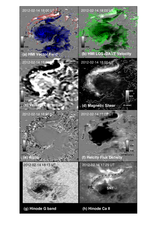
Figure 4: Sub-region R1 on February 14/18:00UT: (a) transverse magnetic field ($B_{t}$) vectors overlaid on LOS magnetic field drawn with polarity inversion line (dashed curve), (b) horizontal velocity vectors showing vortical-like pattern due to rotation of SN1, (c) vertical current ($J_{z}=(\nabla\times\mathbf{B})_{z}/\mu_{0}$) distribution, (d) shear angle map indicates strong shear about the PIL of SP1 and SN1 with their rotation and shear motion of SP1, (e) Alpha ($\alpha=(\nabla\times\mathbf{B})_{z}/B_{z}$) distribution with iso-contours of LOS field indicates overal negative twist of the region (f) helicity flux density map showing negative helicity distribution in the sunspots that is consistent with negative “alpha”, (g) Hinode continuum G-band image, and (h) Hinode chromospheric Ca ii image with the bright flare ribbons of M2.2 at $14/17:20$UT around the PIL.

The vector magnetic field map of the sub-region R1 on February 14/18:00UT is shown in Figure 4(a) along with the map of tracked horizontal velocities of magnetic fluxes in Figure 4(b). The magnetic transverse vectors are seen nearly aligned with the polarity inversion line(PIL, thick dashed curve), implying a large shear along the SP1-SN1 interface. The map of tracked velocities shows the velocity vectors exhibiting spiral or vortical patterns in the penumbral region of SN1 as a fact of its rotation, and the velocity vectors aligned in the opposite direction to that of the magnetic field vectors.

The new emerging positive flux SP1 rotated in the CCW direction, along with a proper motion towards the main flare site R2. It is noteworthy that when the footpoints were dragged along one direction, the corresponding vector magnetic field pointed towards the opposite direction to retain its footpoint connectivity. In the process, the shear in magnetic structures built up. The shear motion along the polarity inversion line (PIL) is an effective mechanism for enhancing non-potentiality of magnetic fields. This can be identified as the alignment of transverse magnetic field vectors along the PIL (Ambastha et al., 1993). Clearly, shear (Equation 1) distribution map shows intense shear about the PIL with the rotation of SN1 and SP1 and proper motion of SN1 as well. This process indeed enhanced the electric currents along PIL as is evident from the the distribution of calculated vertical current $J_{z}$ in frame (c) of Figure 4. Following Zhang (2001), the $J_{z}$ is decomposed to current of chirality $J_{z}^{\rm ch}$ and current of heterogeneity $J_{z}^{\rm h}$, and examined their trend. The average ratio $J_{z}^{\rm ch}$/$J_{z}^{\rm h}$ through out the time is deduced to be 1.11 implying the region is chirally dominated and is approximately consistent with force-free equilibrium. Interestingly, the shear current i.e. $J_{z}^{\rm h}$ follows similar increasing trend with $J_{z}^{\rm ch}$ having correlation coefficient of 0.97, inferring that the rotational motion leads to increase both twist as well as shear contributing to total current $J_{z}$. Moreover, the force free parameter $\alpha=J_{z}/B_{z}$ is having negative distribution (of order $10^{-6}$ m^-1) explaining the chirality with the counter rotation of the constituent sunspots in R1. From the AIA observations of R1, and also as confirmed by STEREO, it is observed that the intermittent mass expulsions turned into fast CMEs in this sub-region.

A map of helicity flux density computed from horizontal flux motions is shown in Figure 4(d). Through out the time interval, the helicity flux distribution is homogeneous with negative (dark) sign and implies left handed sense of chirality, further conforming to the observed CCW rotation of SP1 and SN1. The bipolar flux system having such counter-clock (SP1) and counter-clock (SN1) rotations forms sigmoidal patters which are efficient energy storage mechanisms to account for the flares/CMEs (Canfield et al., 1999). This is also evidenced by the high resolution Hinode G-band continuum image showing filamentary structures (frame (e)) that are consistent with the rotational motion of SP1 and SN1. The corresponding Hinode chromospheric Ca ii image (frame (f)) shows the flare ribbons along the PIL and overlying bright flare loops across the PIL (dashed line) associated with an M-class event of February 14. These observations suggest to infer that the rotational motion of SN1 played a significant role in creating favorable conditions for the eruptions.

The vector magnetic map of sub-region R2 is shown in Figure 5 at the time of X2.2 flare with a smoothed polarity inversion line (thick dashed curve) separating positive and negative LOS magnetic field. This sub-region gave rise to several flares (listed in Table 1) of varying magnitudes including the energetic X2.2 flare along with its associated CME. Importantly, a major portion of the flux (SP2 and SN2) is relatively associated to shearing motion, compared to flux within rotating SP2 itself, therefore this region R2 is shear motion dominated. As in R1, the alignment of $B_{t}$ vectors with PIL in this sub-region also showed strongly sheared magnetic fields. The tracked horizontal velocities (cf., Schuck 2006) displayed strong shearing motion of SP2 along PIL. These motions led to the stressing of field lines and possible flux cancellation as SP2 and SN2 possessed opposite fluxes. The distribution of vertical currents ($J_{z}$), another indicator of large non-potentiality of magnetic structures, too showed strong currents around the PIL in R2 in the form of J-shaped ribbons. High order shear is polarized along the PIL probably due to continuous shear motion of SP2 and rotation. This sub-region is roughly consistent with force-free equilibrium as the average ratio over the time $J_{z}^{\rm ch}$/$J_{z}^{\rm h}$ =1.29 indicating dominant chirality associated current. Nevertheless there exist dominant shear motion with magnetic shear and gradients, $J_{z}^{\rm h}$ does not show increasing trend, but indeed there do observed in $J_{z}^{\rm ch}$ as that in total current $J_{z}$. It means that both rotational as well as proper motions are contributing to $J_{z}^{\rm ch}$ the component that is parallel to to magnetic field. Therefore, the boundary motions in the evolution of the system that is in force-free equilibrium retains it to be in same force-free equilibrium. Distribution of helicity flux is inhomogeneous having mixed polarities and especially during the peak times of some flare events like M6.6 and X2.2, we noticed the negative helicity flux in the existing system of positive helicity flux about the PIL. Injection of such opposite signed helicity is indicative of imminent transient activity. Whereas twisted penumbral fibril structure is seen in the Hinode G-band image on the photosphere, while, the bright chromospheric ribbons from X2.2 flare lying on either side of the PIL are seen in the Hinode Ca ii image.

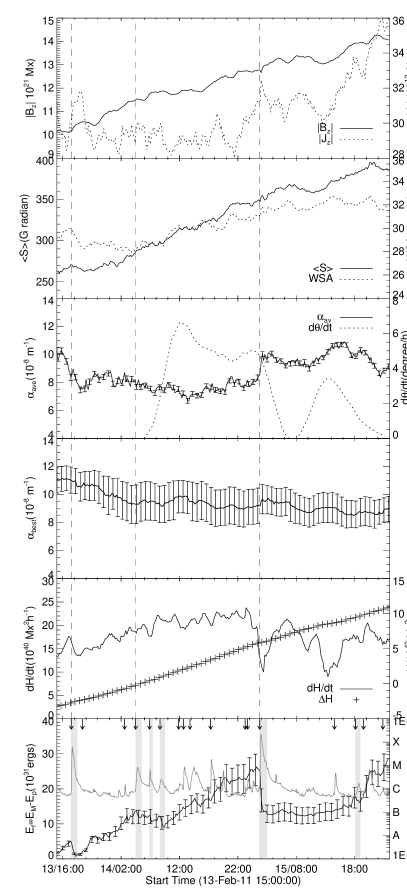
Figure 6: Temporal evolution of various physical parameters characterizing the non-potentiality in sub-regions R1 (left column) and R2 (right column). Arrows in the lower-most panel of the left column mark the CME timings while those in the right column correspond to the GOES-15 flares. The three major flares are marked by dashed vertical lines in all panels on the right column, for reference, while the shaded vertical bars indicate the release of free-energy in step with the onset of flares. Note that all the twist parameters $\alpha_{\rm av}$, $\alpha_{\rm best}$, average shear ($<S>$), and dH/dt has clear correspondence with the rotational profile of the sunspot SN1 implying that sunspot rotation has direct role in increasing the non-potentiality in sub-region R1.

Temporal profiles of the deduced physical parameters for the sub-region R1 are plotted in Figure 6 (left column). The total absolute flux doubled from $5\times 10^{21}$Mx to $9\times 10^{21}$Mx from February 13 to February 15. Thereafter, it showed no significant increase. This increase of flux is gradual which is contributed by emergence of SP1 and gradual evolution of SN1 in a proportion of approximately 1:3. The absolute vertical current also increased along with the flux till February 15, and decreased afterwards. There was a pronounced increase in $|J_{z}|$, from 2.0 to 2.6$\times 10^{12}$A, after 14/14:00UT. The average of shear ($<S>$) and weighted shear angle(WSA) are having similar trend, and explains the $J_{z}$ temporal trend. This might be related to the increasing rotation rate of the sunspot, thereby increasing the shear of horizontal magnetic fields by dragging the foot-points accommodating large field gradients about the PIL.

The sign and magnitude of $\alpha_{\rm av}$ and $\alpha_{\rm best}$ are found to be consistent as both the parameters are equivalent proxies representing the twist. The larger error bars in $\alpha_{\rm best}$ arise due to the $150$G error in the transverse field given to propagate in the fitting procedure (See Eq. 7). The negative sign indicates the left handed twist or chirality. This agrees well with the physically observed CCW rotation of the sub-region consisting of the sunspots SN1 and SP1. The twist proxies, $\alpha_{\rm av}$ and $\alpha_{\rm best}$, showed an increasing trend (in magnitude) with the rotation profile of SP1 (see Figure 3) further corroborating the increase in non-potentiality, as also evident from the absolute vertical current $|J_{z}|$. A similar trend also reflected from the temporal profile of helicity injection rate $dH/dt$ calculated from the physically derived horizontal velocity field of the flux motions. The distribution of helicity flux is homogeneous with negative sign over this region R1 and the helicity injection rate increased (in magnitude) with the rotation rate, reaching a maximum of $-17.52\times 10^{40}$Mx²h^-1. Thereafter it decreased as did the rotation rate. As corona can not accommodate any amount of helicity that is being accumulated continuously, it would try to expel to still outer atmosphere in the form of CMEs so that the system to be stable, therefore explaining the CMEs observed from region R1 of this AR. A total helicity accumulation of $-4.44\times 10^{42}$Mx² was estimated in the sub-region R1 during this period. Since major part of the flux(SN1) is associated to rotational motion, this accumulated helicity is mostly contributed by dominant rotational motion in this sub-region.

The three parameters are different representations of twist or magnetic complexity except the manner in which they are estimated. Increased rotation rate of SN1 seems to increase the twist so does the increasing trend of these parameters. The strong mass expulsions observed in AIA/304Å at 12:50, 17:30, 19:20UT on February 14, turning into CMEs, further strengthen this evidence. This correspondence of the twist parameters $\alpha_{\rm av}$, $\alpha_{\rm best}$,$<S>$, WSA, and $dH/dt$ with the rotational profile of SN1 suggests the predominant role of rotation in the observed expulsions/CMEs (refer to panels a1 and b1 in Figure 2).

Thus we are able to identify the correspondence of the measured twist parameters with the observed rotation of the sunspot in sub-region R1. However, the free-energy deduced for R1 did not show any obvious association with the observed CMEs. We believe that the broad peaks in free-energy profile seen during the CMEs (12:50, 17:30, 19:20UT) might have some relation but a rapid release of energy is not obvious. The maximum mean value of free-energy was estimated around $10^{32}$ ergs; adequate to account for the large eruptions.

Temporal profiles of the deduced physical parameters for the sub-region R2 are plotted in Figure 6 (right column). Absolute flux for this sub-region was much larger in magnitude as compared to that in R1. It increased monotonically from $10\times 10^{21}$Mx to $14\times 10^{21}$Mx. The magnitude of absolute current $J_{z}$ too was correspondingly larger and showed appreciable variations associated with local evolution. Peaks in the electric current profile are noticeable at the times of large flare events, i.e., M6.6 and X2.2. The currents decreased thereafter, implying the build up currents in the preflare phase leads to relaxation of the magnetic field structure by releasing energy during flares. These peaks does not reflect in the $<S>$ and WSA profile because of averaging property of these parameters. Note that WSA is higher by about 7° compared to that of R1 implying high level of non-potentiality over the region. Both the twist proxies, $\alpha_{\rm av}$ and $\alpha_{\rm best}$, agreed in sign and magnitude. Unlike in R1, the positive sign of these parameters represents a positive or right handed twist in R2. A relatively large average value of $\alpha_{\rm av}$ at $8.5\times 10^{-8}$m^-1 is suggestive of a stronger twist present in this sub-region. There seems no corresponding trend of any of these parameters with the rotational profile of SP2 probably complexity in the flux system is not only due to twisting but also shearing of fluxes.

Unlike R1, the sub-region R2 showed positive helicity injection at a much larger rate, with a maximum of $29.11\times 10^{40}$Mx²h^-1. The accumulated helicity too was comparatively larger. A total helicity of $10.27\times 10^{42}$Mx² was injected during the 60h period by the observed flux motions and as a result the coronal helicity is likely to be positive. Within R2, shearing of flux system between SN2 and SP2 is dominated over twisting of single flux system of SP2, therefore it is likely that the accumulated helicity is mostly contributed by the shear motion. This observance is consistent with reports of Liu & Zhang (2006) in AR 10488 having shearing and twisting phases. They claimed that shear motion between two different flux systems indeed the major contributor of helicity injection in that AR.

At the epochs of the M6.6 and X2.2 flares, sharp dips in helicity rate occurred corresponding to the injection of opposite, negative helicity. Existence of such both signs of helicity flux in a single domain is supposed to be sign of triggering transient flare events (Linton et al., 2001; Kusano et al., 2004). However, such an observational evidence of negative or opposite helicity flux may not be real change due to true helicity transfer, it could be flare related transient change effecting the magnetic field measurements. The observed distribution of negative helicity flux coincides spatially and temporally to the reports of possible flare effects on Doppler and magnetic measurements in X2.2 flare (Maurya et al., 2012). A specific study focusing the helicity injection and its behavioral change during flares and CMEs from this AR 11158 in presented in Vemareddy et al. (2012). They showed the change of helicity flux signal due to injection of opposite helicity could be a true change unless there is no impulsive effect of the of the flare on magnetic field measurements. In particular, the localized helicity flux distribution is affected by flare-related transient effects during these M6.6 and X2.2 flare cases having sudden dips in the helicity flux profile as drawn in the figure.

The temporal profile of free-energy is plotted in the bottom frame of Figure 6, along with the GOES X-ray flux. The onset times of flares from the sub-region R2 are marked in this frame. The error bars represent standard deviation of free-energy obtained by changing the origin of coordinate system as explained before, representing the departure from force-freeness and flux balance. It is to note that the AR, as a whole, nearly fulfills the conditions for force-freeness and flux balance ($\leqslant 0.05$). Therefore, the constructed potential field from the extrapolation is not far from these conditions. The integration was carried out over the sub-regions of interest, i.e., R1 and R2, using eq 9. Although the force-free condition was nearly satisfied, a part of field lines from R2 were seen connected to R1 from the coronal AIA images. Hence, the condition for flux balance was not fully obeyed, posing some problem for the applicability of the virial-theorem. Therefore, the derived results are not conclusive enough unless the mean value of free-energy is much larger than the error bars.

The most significant finding of the free-energy plot is the step-down decrease in free energy at the onset of the flares (indicated by the GOES X-ray profile). This provides an unambiguous evidence of energy release during the flares. Magnetic energy is believed to be stored by flux emergence and/or shear motions and is reflected in the form of electric currents. When an instability occurs in the field structure, the excess or free energy is released in the form of flares and CMEs. The flare events having such a correspondence are shown by vertical shaded bars.

As the magnetic fluxes evolved and moved out of the sub-area R2, the fields departed increasingly from the flux-balance condition. Therefore, the free energy derived after the X2.2 flare are increasingly unmeaningful as evident from the large error bars. We estimated that the flux imbalance steadily increased from 5% on February 13 to 16% on February 15. However, the mean value of free energy showed a clear step down decrease at the onset of the X2.2 flare, indicating an appreciable release of energy sufficient to account for this event. Therefore, the relatively large error bars notwithstanding, the variation of free-energy appears to be convincing at the time of this energetic X-class flare.

The changes in potential and total energy estimated during the period from the onset to post-flare phase are given in Table 2 for some flares where we found the step-down decrease in the energy. The difference in available free-energy between the post-flare and the flare onset time giving the amount of energy released during the main flares, are described in the following.

Table 2: Estimated total and potential energies during flares

Flare	Total Energy($E_{T}$ $10^{32}$ergs)		Potential Energy($E_{P}$ $10^{32}$ergs)
	Before Flare	After Flare	Before flare	After flare
M6.6	$1.11\pm 0.39$	$0.69\pm 0.25$	$0.61\pm 0.22$	$0.63\pm 0.24$
X2.2	$4.92\pm 1.58$	$3.67\pm 1.20$	$2.43\pm 0.78$	$2.47\pm 0.79$
C8.3	$3.35\pm 1.06$	$3.16\pm 1.00$	$1.99\pm 0.63$	$1.97\pm 0.63$
C6.6	$3.25\pm 1.03$	$3.20\pm 1.01$	$2.02\pm 0.64$	$2.11\pm 0.67$
C1.8	$3.32\pm 1.05$	$2.97\pm 0.94$	$2.11\pm 0.67$	$2.07\pm 0.66$
C1.7	$2.27\pm 0.79$	$2.29\pm 0.81$	$2.88\pm 0.82$	$2.56\pm 0.08$

The X2.2 flare of February 15/01:44UT: The total energy $E_{T}\approx[4.92\pm 1.58]\times 10^{32}$ erg was estimated on February 15/01:48UT. It decreased to $[3.67\pm 1.20]\times 10^{32}$ erg after the impulsive phase of the flare, i.e., at 02:12UT. The ratio $E_{T}/E_{P}$ of the total energy with the energy of the respective potential state correspond to 2.01 and 1.46 at these two time instants. During this short 24 minute period, the excess energy released was estimated as $[1.05\pm 1.04]\times 10^{32}$erg, sufficient to account for an X-class flare.

The M6.6 flare of February 13/17:28UT: The ratio $E_{T}/E_{P}$ of 1.6 at the onset time of the flare at 17:24UT reduced to 1.08 at 18:12UT, i.e., after the flare. This implies the release of free-energy of $[4.3\pm 1.7]\times 10^{31}$erg, i.e., consistent with the magnitude of the flare.

Similarly, the free-energies released for the C-class events, listed in the Table 1, shown by shaded bars and were estimated as $(1.8\pm 5.9)\times 10^{31}$, $(1.6\pm 5.4)\times 10^{31}$, $(3.7\pm 5.2)\times 10^{31}$ and $(1.1\pm 4.5)\times 10^{31}$erg. These estimated values are not statistically significant as the mean values are smaller than the errors by a factor of two. Because the magnetic energy change is purely due to the change in the boundary conditions, it is expected that even minute changes in the magnetic field corresponding to a C-class flare would reflect in the mean values retaining error bars without much change.

4 Summary and Conclusions

This study suggests that the rotational motions of major sunspots in NOAA AR 11158 were not only related to the transport of magnetic energy and complexity from the low atmosphere to the corona, but also appear to have played a major role in the onset of flares and CMEs. We have attempted to infer the relationship between the observed flux motions, variations in derived physical parameters in association with the dynamical transients, viz., flares and CMEs. A careful analysis of the flux motions leads us to better understand the dynamical nature of the photosphere at the interface between the convection zone where basic dynamo originates and the tenuous corona.

The observations presented here provide a direct evidence for the energization of the solar corona by the emergence and/or dynamics of magnetic flux-tubes that appear as rotating sunspots. This phenomenon is important for understanding how the solar atmosphere attains the conditions necessary for the release of energy and helicity observed in solar flares and CMEs. For a detailed study of various physical parameters characterizing non-potentiality, we selected two sub-regions, R1 and R2, of AR NOAA 11158, which consisted of rotating sunspots. In R1 with the rotating sunspot SN1, the estimated rotation rate is found to have a good correspondence with twist parameters $\alpha_{\rm av}$ and $\alpha_{\rm best}$, $<S>$, and dH/dt. It showed that the intrinsic rotation of the sunspot increased the overall twist in sub-region R1. Major CMEs in R1 occurred on 14 February at 12:50, 17:30, 19:20UT, which coincided well with the timings of large helicity injection rates and twist parameters. As the sunspot’s rotation rate reached the maximum, the fluxes moved with maximum velocities to provide larger complexity in the connectivity. The calculated free-energies, however, did not show good correspondence with the observed CME events, except that broad peaks were observed during these CMEs. This is largely due to violation of flux-balance condition(80%). It is to note that the occurrence of CMEs is also attributed to the new flux emergence (Martin et al., 1985; Zhang et al., 2008). However, the absolute flux profile of R1 does not show such sudden emergence of flux related to emergence of SP1.

No clear relationship of the rotation rate was found with the twist parameters and dH/dt for the sunspot SP2 in R2. Shear motion of SP2 (cf., Figure 1f) seems to be the dominant factor, which obliterates the rotational effect of SP2 on the twist parameters and helicity rate. This shear motion caused the storage of magnetic energy by stressing the field lines. The intermittent release of energy during the observed flares is discernible. A total free-energy of $(1.05\pm 1.04)\times 10^{32}$erg is released during the X2.2 flare. This is three times larger than the derived energy from coronal magnetic field extrapolations by Sun et al. (2012) over the entire AR. Spectral line-profile reversals occurred during the impulsive phase of this flare affecting the magnetic and velocity field measurements, as reported recently by Maurya et al. (2012). As a result, the injected helicity rate showed an impulsive negative peak by the sudden appearance of negative helicity density indicating flare-related transient effect (cf., Figure 5d).

The M6.6 flare of February 13/17:28UT was another large but less impulsive event which released $(4.3\pm 1.7)\times 10^{31}$erg of energy in the 48 minute period. Step down decrease of free-energy was found not only during the two large flares, but also in some flares of smaller magnitude. This reveals the storage and release of energy in the flares occurring in sub-region R2. It is to mention that we have not carried out the analysis of errors due to the spectro-polarimetric as well as random noise and their effects on the free-energy estimation, as there is no established method available on the data set as yet. Moreover, the estimation of free-energy suffers by the departure from the validity conditions of virial theorem due to the selection of small sized areas of the sub-regions.

The accumulated helicity contributed by the rotational motion of the sunspot can also be obtained as

$$\Delta H=-\frac{1}{2\pi}\Delta\theta\Phi^{2},$$ (10)

where $\Phi$ is the magnetic flux and $\Delta\theta$ is the total rotation angle of the sunspot. Since the sunspot SN1 rotated by $\approx 160\arcdeg$ during the 60h period of our study, and assuming the average magnetic flux of this sunspot as $3.5\times 10^{21}$Mx, the accumulated helicity by rotation is estimated as -$5.44\times 10^{42}$Mx². This is consistent with the derived value of -$4.44\times 10^{42}$Mx² from the tracked velocities of the fluxes.

Thus, this study demonstrates that both shear (dominated in R2) and rotational (dominated in R1) motions of the observed fluxes enhanced the magnetic non-potentiality of the active region by injecting helicity. This helped in increasing the free energy of the AR’s magnetic field by increasing the overall complexity leading to the conditions favorable for the eruptions. The deduced physical parameters describing the level of magnetic non-potentiality and the free energy showed a reasonably good correspondence with the observed transient activity of the AR. This study also provides a clear signatures of energy release during the major, energetic transients of the AR.

Figure 1: HMI intensity images showing the evolution of AR NOAA 11158 during six day time period. The main sunspots are labeled by SP/N* in (d) along with the LOS magnetic field contours overlaid in red (blue) color at 150(-150)G levels in panel(also in subsequent figures unless specified) (e). Proper motions of individual sunspots are traced along the arrowed curves as in panel (f). The two rectangular boxes mark the selected sub-regions R1 and R2 for further study.

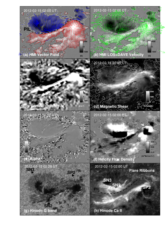
Figure 5: Sub-region R2 on February 15/02:00UT: (a) transverse magnetic field ($B_{t}$) vectors overlaid on LOS magnetic field with PIL separating positive and negative polarities, (b) tracked horizontal velocity vectors overplotted on LOS magnetic field, (c) Vertical current distribution ($J_{z}$) showing intense currents accumulated on either side of PIL with the shear motion of SP2, (d) Shear angle map also implies strong shear polarized about the PIL with the continuous shear motion of SP2, (e) Distribution of twist parameter “alpha” indicates positive twist of the region, (f) helicity flux density map with intense negative helicity flux about PIL probably due to flare-effects on magnetic field measurements, (g) Hinode continuum G-band, and (h) Hinode chromospheric Ca ii image showing the flare ribbons of $X2.2$ around the PIL (dashed curve).

References

- Ambastha et al. (1993) Ambastha, A., Hagyard, M. J., & West, E. A. 1993, Sol. Phys., 148, 277
- Bhatnagar (1967) Bhatnagar, A. 1967, Kodaikanal Observ. Bull.
- Borrero et al. (2011) Borrero, J. M., Tomczyk, S., Kubo, M., Socas-Navarro, H., Schou, J., Couvidat, S., & Bogart, R. 2011, Sol. Phys., 273, 267
- Brown et al. (2003) Brown, D. S., Nightingale, R. W., Alexander, D., Schrijver, C. J., Metcalf, T. R., Shine, R. A., Title, A. M., & Wolfson, C. J. 2003, Sol. Phys., 216, 79
- Canfield et al. (1999) Canfield, R. C., Hudson, H. S., & McKenzie, D. E. 1999, Geophys. Res. Lett., 26, 627
- Chandrasekhar (1961) Chandrasekhar, S. 1961, Hydrodynamic and hydromagnetic stability, ed. Chandrasekhar, S.
- Evershed (1910) Evershed, J. 1910, MNRAS, 70, 217
- Freeland & Handy (1998) Freeland, S. L., & Handy, B. N. 1998, Sol. Phys., 182, 497
- Gary (1989) Gary, G. A. 1989, ApJS, 69, 323
- Gary (2001) —. 2001, Sol. Phys., 203, 71
- Hagino & Sakurai (2004) Hagino, M., & Sakurai, T. 2004, PASJ, 56, 831
- Hiremath et al. (2005) Hiremath, K. M., Suryanarayana, G. S., & Lovely, M. R. 2005, A&A, 437, 297
- Hoeksema & et al. (2012) Hoeksema, J. T., & et al. 2012, Sol. Phys., To be Submitted
- Howard et al. (1990) Howard, R. F., Harvey, J. W., & Forgach, S. 1990, Sol. Phys., 130, 295
- Jiang et al. (2012) Jiang, Y., Zheng, R., Yang, J., Hong, J., Yi, B., & Yang, D. 2012, ApJ, 744, 50
- Kusano et al. (2004) Kusano, K., Maeshiro, T., Yokoyama, T., & Sakurai, T. 2004, ApJ, 610, 537
- Leka & Barnes (2003) Leka, K. D., & Barnes, G. 2003, ApJ, 595, 1277
- Leka et al. (2009) Leka, K. D., Barnes, G., Crouch, A. D., Metcalf, T. R., Gary, G. A., Jing, J., & Liu, Y. 2009, Sol. Phys., 260, 83
- Lemen et al. (2012) Lemen, J. R., Title, A. M., Akin, D. J., Boerner, P. F., & et al. 2012, Sol. Phys., 275, 17
- Linton et al. (2001) Linton, M. G., Dahlburg, R. B., & Antiochos, S. K. 2001, ApJ, 553, 905
- Liu & Zhang (2006) Liu, J., & Zhang, H. 2006, Sol. Phys., 234, 21
- Low (1982) Low, B. C. 1982, Sol. Phys., 77, 43
- Martin et al. (1985) Martin, S. F., Livi, S. H. B., & Wang, J. 1985, Australian Journal of Physics, 38, 929
- Maurya et al. (2012) Maurya, R. A., Vemareddy, P., & Ambastha, A. 2012, ApJ, 747, 134
- McIntosh (1981) McIntosh, P. S. 1981, in The Physics of Sunspots, ed. L. E. Cram & J. H. Thomas, 7–54
- Metcalf (1994) Metcalf, T. R. 1994, Sol. Phys., 155, 235
- Metcalf et al. (1995) Metcalf, T. R., Jiao, L., McClymont, A. N., Canfield, R. C., & Uitenbroek, H. 1995, ApJ, 439, 474
- Metcalf et al. (2005) Metcalf, T. R., Leka, K. D., & Mickey, D. L. 2005, ApJ, 623, L53
- Molodensky (1974) Molodensky, M. M. 1974, Sol. Phys., 39, 393
- Pariat et al. (2005) Pariat, E., Démoulin, P., & Berger, M. A. 2005, A&A, 439, 1191
- Pevtsov et al. (1994) Pevtsov, A. A., Canfield, R. C., & Metcalf, T. R. 1994, ApJ, 425, L117
- Schou et al. (2012) Schou, J., Scherrer, P. H., Bush, R. I., Wachter, R., & et al. 2012, Sol. Phys., 275, 229
- Schuck (2006) Schuck, P. W. 2006, ApJ, 646, 1358
- Sun et al. (2012) Sun, X., Hoeksema, J. T., Liu, Y., Wiegelmann, T., Hayashi, K., Chen, Q., & Thalmann, J. 2012, ApJ, 748, 77
- Tian & Alexander (2006) Tian, L., & Alexander, D. 2006, Sol. Phys., 233, 29
- Tian et al. (2008) Tian, L., Alexander, D., & Nightingale, R. 2008, ApJ, 684, 747
- Tsuneta et al. (2008) Tsuneta, S., Ichimoto, K., Katsukawa, Y., Nagata, S., & et al. 2008, Sol. Phys., 249, 167
- Vemareddy et al. (2012) Vemareddy, P., Ambastha, A., Maurya, R. A., & Chae, J. 2012, ArXiv e-prints
- Wang et al. (1994) Wang, H., Ewell, Jr., M. W., Zirin, H., & Ai, G. 1994, ApJ, 424, 436
- Yan et al. (2008) Yan, X.-L., Qu, Z.-Q., & Kong, D.-F. 2008, MNRAS, 391, 1887
- Yan et al. (2009) Yan, X.-L., Qu, Z.-Q., Xu, C.-L., Xue, Z.-K., & Kong, D.-F. 2009, Research in Astronomy and Astrophysics, 9, 596
- Zhang (2001) Zhang, H. 2001, ApJ, 557, L71
- Zhang et al. (2007) Zhang, J., Li, L., & Song, Q. 2007, ApJ, 662, L35
- Zhang et al. (2008) Zhang, Y., Liu, J., & Zhang, H. 2008, Sol. Phys., 247, 39