On a non-local problem for parabolic-hyperbolic equation with three lines of type changing
Karimov E.T., Sotvoldiev A.I.
E-mail: erkinjon@gmail.com,akm0111@inbox.ru
Institute of Mathematics, National University of Uzbekistan named after Mirzo Ulughbek (Tashkent, Uzbekistan)
MSC 2000: 35M10
Keywords: parabolic-hyperbolic equation; non-local condition; Volterra integral equation
Abstract. In the present work we investigate a boundary problem with non-local conditions, connecting values of seeking function on various characteristics for parabolic-hyperbolic equation with three lines of type changing. The considered problem is equivalently reduced to the system of Volterra integral equations of the second kind.
Consider an equation
0 = { u x x − u y , ( x , y ) ∈ Ω 0 , u x x − u y y , ( x , y ) ∈ Ω i ( i = 1 , 3 ¯ ) 0=\left\{\begin{gathered}{u_{xx}}-{u_{y}},\,\,\,\,\,\,\left({x,y}\right)\in{\Omega_{0}},\hfill\\
{u_{xx}}-{u_{yy}},\,\,\,\,\,\left({x,y}\right)\in{\Omega_{i}}\,\left({i=\overline{1,3}}\right)\hfill\\
\end{gathered}\right. ( 1 ) 1
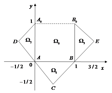
in the domain Ω = Ω 0 ∪ Ω 1 ∪ Ω 2 ∪ Ω 3 ∪ A B ∪ A A 0 ∪ B B 0 Ω subscript Ω 0 subscript Ω 1 subscript Ω 2 subscript Ω 3 𝐴 𝐵 𝐴 subscript 𝐴 0 𝐵 subscript 𝐵 0 \Omega={\Omega_{0}}\cup{\Omega_{1}}\cup{\Omega_{2}}\cup{\Omega_{3}}\cup AB\cup A{A_{0}}\cup B{B_{0}}
Figure 1: Domain Ω Ω \Omega
Problem AS. Find a regular solution of the equation (1) in the domain Ω Ω \Omega
a 1 ( t ) u ( − t , t ) + a 2 ( t ) u ( t , − t ) = a 3 ( t ) , 0 ⩽ t ⩽ 1 2 , formulae-sequence subscript 𝑎 1 𝑡 𝑢 𝑡 𝑡 subscript 𝑎 2 𝑡 𝑢 𝑡 𝑡 subscript 𝑎 3 𝑡 0 𝑡 1 2 {a_{1}}\left(t\right)u\left({-t,t}\right)+{a_{2}}\left(t\right)u\left({t,-t}\right)={a_{3}}\left(t\right),\,\,0\leqslant t\leqslant\frac{1}{2}, ( 2 ) 2
b 1 ( t ) u ( t , t − 1 ) + b 2 ( t ) u ( 2 − t , 1 − t ) = b 3 ( t ) , 1 2 ⩽ t ⩽ 1 , formulae-sequence subscript 𝑏 1 𝑡 𝑢 𝑡 𝑡 1 subscript 𝑏 2 𝑡 𝑢 2 𝑡 1 𝑡 subscript 𝑏 3 𝑡 1 2 𝑡 1 {b_{1}}\left(t\right)u\left({t,t-1}\right)+{b_{2}}\left(t\right)u\left({2-t,1-t}\right)={b_{3}}\left(t\right),\,\,\frac{1}{2}\leqslant t\leqslant 1, ( 3 ) 3
c 1 ( t ) ( u x + u y ) ( t − 1 , t ) + c 2 ( t ) ( u x − u y ) ( 2 − t , t ) = c 3 ( t ) , 1 2 < t < 1 . formulae-sequence subscript 𝑐 1 𝑡 subscript 𝑢 𝑥 subscript 𝑢 𝑦 𝑡 1 𝑡 subscript 𝑐 2 𝑡 subscript 𝑢 𝑥 subscript 𝑢 𝑦 2 𝑡 𝑡 subscript 𝑐 3 𝑡 1 2 𝑡 1 {c_{1}}\left(t\right)\left({{u_{x}}+{u_{y}}}\right)\left({t-1,t}\right)+{c_{2}}\left(t\right)\left({{u_{x}}-{u_{y}}}\right)\left({2-t,t}\right)={c_{3}}\left(t\right),\,\,\frac{1}{2}<t<1. ( 4 ) 4
Here a i ( t ) , b i ( t ) , c i ( t ) ( i = 1 , 3 ¯ ) subscript 𝑎 𝑖 𝑡 subscript 𝑏 𝑖 𝑡 subscript 𝑐 𝑖 𝑡 𝑖 ¯ 1 3
{a_{i}}\left(t\right),{b_{i}}\left(t\right),{c_{i}}\left(t\right)\,\left({i=\overline{1,3}}\right)
a 1 ( 0 ) + a 2 ( 0 ) ≠ 0 , b 1 ( 1 ) + b 2 ( 1 ) ≠ 0 , a 1 2 ( t ) + a 2 2 ( t ) > 0 , b 1 2 ( t ) + b 2 2 ( t ) > 0 , c 1 2 ( t ) + c 2 2 ( t ) > 0 , a 1 2 + b 2 2 > 0 , a 2 2 + b 1 2 > 0 . formulae-sequence subscript 𝑎 1 0 subscript 𝑎 2 0 0 formulae-sequence subscript 𝑏 1 1 subscript 𝑏 2 1 0 formulae-sequence superscript subscript 𝑎 1 2 𝑡 superscript subscript 𝑎 2 2 𝑡 0 formulae-sequence superscript subscript 𝑏 1 2 𝑡 superscript subscript 𝑏 2 2 𝑡 0 formulae-sequence superscript subscript 𝑐 1 2 𝑡 superscript subscript 𝑐 2 2 𝑡 0 formulae-sequence superscript subscript 𝑎 1 2 superscript subscript 𝑏 2 2 0 superscript subscript 𝑎 2 2 superscript subscript 𝑏 1 2 0 \begin{gathered}{a_{1}}\left(0\right)+{a_{2}}\left(0\right)\neq 0,\,{b_{1}}\left(1\right)+{b_{2}}\left(1\right)\neq 0,\,a_{1}^{2}\left(t\right)+a_{2}^{2}\left(t\right)>0,\,b_{1}^{2}\left(t\right)+b_{2}^{2}\left(t\right)>0,\hfill\\
c_{1}^{2}\left(t\right)+c_{2}^{2}\left(t\right)>0,\,a_{1}^{2}+b_{2}^{2}>0,\,a_{2}^{2}+b_{1}^{2}>0.\hfill\\
\end{gathered}
Note, boundary problems for parabolic-hyperbolic equations with two lines of type changing were investigated in the works [1-4], and with three lines of type changing in the papers [5-6]. Distinctive side of the present work is non-local condition, which connect values of seeking function on various characteristics. It makes very difficult the reduction of the considered problem to the system of integral equations and we need special algorithm for solving this problem.
In the domain Ω 1 subscript Ω 1 {\Omega_{1}} u ( x , 0 ) = τ 1 ( x ) 𝑢 𝑥 0 subscript 𝜏 1 𝑥 u\left({x,0}\right)={\tau_{1}}\left(x\right) u y ( x , 0 ) = ν 1 ( x ) subscript 𝑢 𝑦 𝑥 0 subscript 𝜈 1 𝑥 {u_{y}}\left({x,0}\right)={\nu_{1}}\left(x\right)
2 u ( x , y ) = τ 1 ( x + y ) + τ 1 ( x − y ) + ∫ x − y x + y ν 1 ( z ) 𝑑 z . 2 𝑢 𝑥 𝑦 subscript 𝜏 1 𝑥 𝑦 subscript 𝜏 1 𝑥 𝑦 superscript subscript 𝑥 𝑦 𝑥 𝑦 subscript 𝜈 1 𝑧 differential-d 𝑧 2u\left({x,y}\right)={\tau_{1}}\left({x+y}\right)+{\tau_{1}}\left({x-y}\right)+\int\limits_{x-y}^{x+y}{{\nu_{1}}\left(z\right)dz}. ( 5 ) 5
Assuming in condition (2)
u ( − t , t ) = φ 1 ( t ) , 0 ⩽ t ⩽ 1 2 , formulae-sequence 𝑢 𝑡 𝑡 subscript 𝜑 1 𝑡 0 𝑡 1 2 u\left({-t,t}\right)={\varphi_{1}}\left(t\right),\,\,\,0\leqslant t\leqslant\frac{1}{2}, ( 6 ) 6
as given, from (5) we find
τ 1 ′ ( t ) = ν 1 ( t ) + ( 2 [ a 3 ( t 2 ) − a 1 ( t 2 ) φ 1 ( t 2 ) ] a 2 ( t 2 ) ) ′ , 0 < t < 1 . formulae-sequence subscript superscript 𝜏 ′ 1 𝑡 subscript 𝜈 1 𝑡 superscript 2 delimited-[] subscript 𝑎 3 𝑡 2 subscript 𝑎 1 𝑡 2 subscript 𝜑 1 𝑡 2 subscript 𝑎 2 𝑡 2 ′ 0 𝑡 1 {\tau^{\prime}_{1}}\left(t\right)={\nu_{1}}\left(t\right)+{\left({\frac{{2\left[{{a_{3}}\left({\frac{t}{2}}\right)-{a_{1}}\left({\frac{t}{2}}\right){\varphi_{1}}\left({\frac{t}{2}}\right)}\right]}}{{{a_{2}}\left({\frac{t}{2}}\right)}}}\right)^{\prime}},\,\,\,\,0<t<1. ( 7 ) 7
In condition (3) introduce designation
u ( 2 − t , 1 − t ) = φ 2 ( t ) , 1 2 ⩽ t ⩽ 1 , formulae-sequence 𝑢 2 𝑡 1 𝑡 subscript 𝜑 2 𝑡 1 2 𝑡 1 u\left({2-t,1-t}\right)={\varphi_{2}}\left(t\right),\,\,\,\frac{1}{2}\leqslant t\leqslant 1, ( 8 ) 8
and from (5) we get
τ 1 ′ ( t ) = − ν 1 ( t ) + ( 2 [ b 3 ( t + 1 2 ) − b 2 ( t + 1 2 ) φ 2 ( t + 1 2 ) ] b 1 ( t + 1 2 ) ) ′ , 0 < t < 1 . formulae-sequence subscript superscript 𝜏 ′ 1 𝑡 subscript 𝜈 1 𝑡 superscript 2 delimited-[] subscript 𝑏 3 𝑡 1 2 subscript 𝑏 2 𝑡 1 2 subscript 𝜑 2 𝑡 1 2 subscript 𝑏 1 𝑡 1 2 ′ 0 𝑡 1 {\tau^{\prime}_{1}}\left(t\right)=-{\nu_{1}}\left(t\right)+{\left({\frac{{2\left[{{b_{3}}\left({\frac{{t+1}}{2}}\right)-{b_{2}}\left({\frac{{t+1}}{2}}\right){\varphi_{2}}\left({\frac{{t+1}}{2}}\right)}\right]}}{{{b_{1}}\left({\frac{{t+1}}{2}}\right)}}}\right)^{\prime}},\,\,\,\,0<t<1. ( 9 ) 9
From (7) and (9) it follows that
τ 1 ′ ( t ) = ( a 3 ( t 2 ) − a 1 ( t 2 ) φ 1 ( t 2 ) a 2 ( t 2 ) ) ′ + ( b 3 ( t + 1 2 ) − b 2 ( t + 1 2 ) φ 2 ( t + 1 2 ) b 1 ( t + 1 2 ) ) ′ , 0 < t < 1 . formulae-sequence subscript superscript 𝜏 ′ 1 𝑡 superscript subscript 𝑎 3 𝑡 2 subscript 𝑎 1 𝑡 2 subscript 𝜑 1 𝑡 2 subscript 𝑎 2 𝑡 2 ′ superscript subscript 𝑏 3 𝑡 1 2 subscript 𝑏 2 𝑡 1 2 subscript 𝜑 2 𝑡 1 2 subscript 𝑏 1 𝑡 1 2 ′ 0 𝑡 1 {\tau^{\prime}_{1}}\left(t\right)={\left({\frac{{{a_{3}}\left({\frac{t}{2}}\right)-{a_{1}}\left({\frac{t}{2}}\right){\varphi_{1}}\left({\frac{t}{2}}\right)}}{{{a_{2}}\left({\frac{t}{2}}\right)}}}\right)^{\prime}}+{\left({\frac{{{b_{3}}\left({\frac{{t+1}}{2}}\right)-{b_{2}}\left({\frac{{t+1}}{2}}\right){\varphi_{2}}\left({\frac{{t+1}}{2}}\right)}}{{{b_{1}}\left({\frac{{t+1}}{2}}\right)}}}\right)^{\prime}},\,\,\,\,0<t<1. ( 10 ) 10
Solution of the Cauchy problem in the domain Ω 2 subscript Ω 2 {\Omega_{2}} u ( 0 , y ) = τ 2 ( y ) 𝑢 0 𝑦 subscript 𝜏 2 𝑦 u\left({0,y}\right)={\tau_{2}}\left(y\right) u x ( 0 , y ) = ν 2 ( y ) subscript 𝑢 𝑥 0 𝑦 subscript 𝜈 2 𝑦 {u_{x}}\left({0,y}\right)={\nu_{2}}\left(y\right)
2 u ( x , y ) = τ 2 ( y + x ) + τ 2 ( y − x ) + ∫ y − x y + x ν 2 ( z ) 𝑑 z . 2 𝑢 𝑥 𝑦 subscript 𝜏 2 𝑦 𝑥 subscript 𝜏 2 𝑦 𝑥 superscript subscript 𝑦 𝑥 𝑦 𝑥 subscript 𝜈 2 𝑧 differential-d 𝑧 2u\left({x,y}\right)={\tau_{2}}\left({y+x}\right)+{\tau_{2}}\left({y-x}\right)+\int\limits_{y-x}^{y+x}{{\nu_{2}}\left(z\right)dz}. ( 11 ) 11
Considering (6) from (11) we obtain
τ 2 ′ ( t ) = ν 2 ( t ) + φ 1 ′ ( t 2 ) , 0 < t < 1 . formulae-sequence subscript superscript 𝜏 ′ 2 𝑡 subscript 𝜈 2 𝑡 subscript superscript 𝜑 ′ 1 𝑡 2 0 𝑡 1 {\tau^{\prime}_{2}}\left(t\right)={\nu_{2}}\left(t\right)+{\varphi^{\prime}_{1}}\left({\frac{t}{2}}\right),\,\,0<t<1. ( 12 ) 12
In condition (4) introduce another designation
( u x − u y ) ( 2 − t , t ) = φ 3 ( t ) , 1 2 < t < 1 . formulae-sequence subscript 𝑢 𝑥 subscript 𝑢 𝑦 2 𝑡 𝑡 subscript 𝜑 3 𝑡 1 2 𝑡 1 \left({{u_{x}}-{u_{y}}}\right)\left({2-t,t}\right)={\varphi_{3}}\left(t\right),\,\,\frac{1}{2}<t<1. ( 13 ) 13
Then from (11) we get
c 3 ( t + 1 2 ) − c 2 ( t + 1 2 ) φ 3 ( t + 1 2 ) c 1 ( t + 1 2 ) = τ 2 ′ ( t ) + ν 2 ( t ) , 0 < t < 1 . formulae-sequence subscript 𝑐 3 𝑡 1 2 subscript 𝑐 2 𝑡 1 2 subscript 𝜑 3 𝑡 1 2 subscript 𝑐 1 𝑡 1 2 subscript superscript 𝜏 ′ 2 𝑡 subscript 𝜈 2 𝑡 0 𝑡 1 \frac{{{c_{3}}\left({\frac{{t+1}}{2}}\right)-{c_{2}}\left({\frac{{t+1}}{2}}\right){\varphi_{3}}\left({\frac{{t+1}}{2}}\right)}}{{{c_{1}}\left({\frac{{t+1}}{2}}\right)}}={\tau^{\prime}_{2}}\left(t\right)+{\nu_{2}}\left(t\right),\,\,0<t<1. ( 14 ) 14
From (12) and (14) we deduce
2 τ 2 ′ ( t ) = φ 1 ′ ( t 2 ) + c 3 ( t + 1 2 ) − c 2 ( t + 1 2 ) φ 3 ( t + 1 2 ) c 1 ( t + 1 2 ) , 0 < t < 1 . formulae-sequence 2 subscript superscript 𝜏 ′ 2 𝑡 subscript superscript 𝜑 ′ 1 𝑡 2 subscript 𝑐 3 𝑡 1 2 subscript 𝑐 2 𝑡 1 2 subscript 𝜑 3 𝑡 1 2 subscript 𝑐 1 𝑡 1 2 0 𝑡 1 2{\tau^{\prime}_{2}}\left(t\right)={\varphi^{\prime}_{1}}\left({\frac{t}{2}}\right)+\frac{{{c_{3}}\left({\frac{{t+1}}{2}}\right)-{c_{2}}\left({\frac{{t+1}}{2}}\right){\varphi_{3}}\left({\frac{{t+1}}{2}}\right)}}{{{c_{1}}\left({\frac{{t+1}}{2}}\right)}},\,\,0<t<1. ( 15 ) 15
Solution of the Cauchy problem with data u ( 1 , y ) = τ 3 ( y ) , u x ( 1 , y ) = ν 3 ( y ) formulae-sequence 𝑢 1 𝑦 subscript 𝜏 3 𝑦 subscript 𝑢 𝑥 1 𝑦 subscript 𝜈 3 𝑦 u\left({1,y}\right)={\tau_{3}}\left(y\right),\,{u_{x}}\left({1,y}\right)={\nu_{3}}\left(y\right) Ω 3 subscript Ω 3 {\Omega_{3}}
2 u ( x , y ) = τ 3 ( y + x − 1 ) + τ 2 ( y − x + 1 ) + ∫ y − x + 1 y + x − 1 ν 3 ( z ) 𝑑 z . 2 𝑢 𝑥 𝑦 subscript 𝜏 3 𝑦 𝑥 1 subscript 𝜏 2 𝑦 𝑥 1 superscript subscript 𝑦 𝑥 1 𝑦 𝑥 1 subscript 𝜈 3 𝑧 differential-d 𝑧 2u\left({x,y}\right)={\tau_{3}}\left({y+x-1}\right)+{\tau_{2}}\left({y-x+1}\right)+\int\limits_{y-x+1}^{y+x-1}{{\nu_{3}}\left(z\right)dz}. ( 16 ) 16
Using (8) and (13) from (16), after some evaluations one can get
2 τ 3 ′ ( t ) = − φ 2 ′ ( 2 − t 2 ) − φ 3 ( t + 1 2 ) , 0 < t < 1 . formulae-sequence 2 subscript superscript 𝜏 ′ 3 𝑡 subscript superscript 𝜑 ′ 2 2 𝑡 2 subscript 𝜑 3 𝑡 1 2 0 𝑡 1 2{\tau^{\prime}_{3}}\left(t\right)=-{\varphi^{\prime}_{2}}\left({\frac{{2-t}}{2}}\right)-{\varphi_{3}}\left({\frac{{t+1}}{2}}\right),\,\,0<t<1. ( 17 ) 17
Further, from the equation (1) we pass to the limit at y → + 0 → 𝑦 0 y\to+0
τ 1 ′′ ( t ) − τ 1 ′ ( t ) = − ( 2 [ a 3 ( t 2 ) − a 1 ( t 2 ) φ 1 ( t 2 ) ] a 2 ( t 2 ) ) ′ . subscript superscript 𝜏 ′′ 1 𝑡 subscript superscript 𝜏 ′ 1 𝑡 superscript 2 delimited-[] subscript 𝑎 3 𝑡 2 subscript 𝑎 1 𝑡 2 subscript 𝜑 1 𝑡 2 subscript 𝑎 2 𝑡 2 ′ {\tau^{\prime\prime}_{1}}\left(t\right)-{\tau^{\prime}_{1}}\left(t\right)=-{\left({\frac{{2\left[{{a_{3}}\left({\frac{t}{2}}\right)-{a_{1}}\left({\frac{t}{2}}\right){\varphi_{1}}\left({\frac{t}{2}}\right)}\right]}}{{{a_{2}}\left({\frac{t}{2}}\right)}}}\right)^{\prime}}. ( 18 ) 18
Solution of the equation (18) together with conditions
τ 1 ( 0 ) = a 3 ( 0 ) a 1 ( 0 ) + a 2 ( 0 ) , τ 1 ( 1 ) = b 3 ( 1 ) b 1 ( 1 ) + b 2 ( 1 ) , formulae-sequence subscript 𝜏 1 0 subscript 𝑎 3 0 subscript 𝑎 1 0 subscript 𝑎 2 0 subscript 𝜏 1 1 subscript 𝑏 3 1 subscript 𝑏 1 1 subscript 𝑏 2 1 {\tau_{1}}\left(0\right)=\frac{{{a_{3}}\left(0\right)}}{{{a_{1}}\left(0\right)+{a_{2}}\left(0\right)}},\,\,\,{\tau_{1}}\left(1\right)=\frac{{{b_{3}}\left(1\right)}}{{{b_{1}}\left(1\right)+{b_{2}}\left(1\right)}}, ( 19 ) 19
which reduced from (2) and (3), can be represented as
τ 1 ( x ) = a 3 ( 0 ) a 1 ( 0 ) + a 2 ( 0 ) + x [ b 3 ( 1 ) b 1 ( 1 ) + b 2 ( 1 ) − a 3 ( 0 ) a 1 ( 0 ) + a 2 ( 0 ) ] + + ∫ 0 1 G ( x , t ) [ b 3 ( 1 ) b 1 ( 1 ) + b 2 ( 1 ) − a 3 ( 0 ) a 1 ( 0 ) + a 2 ( 0 ) ] 𝑑 t − − ∫ 0 1 G ( x , t ) ( 2 [ a 3 ( t 2 ) − a 1 ( t 2 ) φ 1 ( t 2 ) ] a 2 ( t 2 ) ) ′ 𝑑 t , 0 ⩽ x ⩽ 1 , formulae-sequence subscript 𝜏 1 𝑥 subscript 𝑎 3 0 subscript 𝑎 1 0 subscript 𝑎 2 0 𝑥 delimited-[] subscript 𝑏 3 1 subscript 𝑏 1 1 subscript 𝑏 2 1 subscript 𝑎 3 0 subscript 𝑎 1 0 subscript 𝑎 2 0 superscript subscript 0 1 𝐺 𝑥 𝑡 delimited-[] subscript 𝑏 3 1 subscript 𝑏 1 1 subscript 𝑏 2 1 subscript 𝑎 3 0 subscript 𝑎 1 0 subscript 𝑎 2 0 differential-d 𝑡 superscript subscript 0 1 𝐺 𝑥 𝑡 superscript 2 delimited-[] subscript 𝑎 3 𝑡 2 subscript 𝑎 1 𝑡 2 subscript 𝜑 1 𝑡 2 subscript 𝑎 2 𝑡 2 ′ differential-d 𝑡 0 𝑥 1 \begin{gathered}{\tau_{1}}\left(x\right)=\frac{{{a_{3}}\left(0\right)}}{{{a_{1}}\left(0\right)+{a_{2}}\left(0\right)}}+x\left[{\frac{{{b_{3}}\left(1\right)}}{{{b_{1}}\left(1\right)+{b_{2}}\left(1\right)}}-\frac{{{a_{3}}\left(0\right)}}{{{a_{1}}\left(0\right)+{a_{2}}\left(0\right)}}}\right]+\hfill\\
+\int\limits_{0}^{1}{G\left({x,t}\right)}\left[{\frac{{{b_{3}}\left(1\right)}}{{{b_{1}}\left(1\right)+{b_{2}}\left(1\right)}}-\frac{{{a_{3}}\left(0\right)}}{{{a_{1}}\left(0\right)+{a_{2}}\left(0\right)}}}\right]dt-\hfill\\
-\int\limits_{0}^{1}{G\left({x,t}\right)}{\left({\frac{{2\left[{{a_{3}}\left({\frac{t}{2}}\right)-{a_{1}}\left({\frac{t}{2}}\right){\varphi_{1}}\left({\frac{t}{2}}\right)}\right]}}{{{a_{2}}\left({\frac{t}{2}}\right)}}}\right)^{\prime}}dt,\,\,\,\,0\leqslant x\leqslant 1,\hfill\\
\end{gathered} ( 20 ) 20
where G ( x , t ) 𝐺 𝑥 𝑡 G\left({x,t}\right)
Continuing to assume the function φ 1 subscript 𝜑 1 {\varphi_{1}} φ 2 subscript 𝜑 2 {\varphi_{2}} φ 1 subscript 𝜑 1 {\varphi_{1}} Ω 0 subscript Ω 0 {\Omega_{0}} τ j subscript 𝜏 𝑗 {\tau_{j}} ν j subscript 𝜈 𝑗 {\nu_{j}} ( j = 2 , 3 ) 𝑗 2 3
\left({j=2,3}\right)
τ ′ 2 ( y ) = ∫ 0 y τ ′ 3 ( η ) N ( 0 , y , 1 , η ) 𝑑 η − ∫ 0 y τ ′ 2 ( η ) N ( 0 , y , 0 , η ) 𝑑 η + F 1 ( y ) , τ ′ 3 ( y ) = ∫ 0 y τ ′ 3 ( η ) N ( 1 , y , 1 , η ) 𝑑 η − ∫ 0 y τ ′ 2 ( η ) N ( 1 , y , 0 , η ) 𝑑 η + F 2 ( y ) , formulae-sequence subscript superscript 𝜏 ′ 2 𝑦 superscript subscript 0 𝑦 subscript superscript 𝜏 ′ 3 𝜂 𝑁 0 𝑦 1 𝜂 differential-d 𝜂 superscript subscript 0 𝑦 subscript superscript 𝜏 ′ 2 𝜂 𝑁 0 𝑦 0 𝜂 differential-d 𝜂 subscript 𝐹 1 𝑦 subscript superscript 𝜏 ′ 3 𝑦 superscript subscript 0 𝑦 subscript superscript 𝜏 ′ 3 𝜂 𝑁 1 𝑦 1 𝜂 differential-d 𝜂 superscript subscript 0 𝑦 subscript superscript 𝜏 ′ 2 𝜂 𝑁 1 𝑦 0 𝜂 differential-d 𝜂 subscript 𝐹 2 𝑦 \begin{gathered}{{\tau^{\prime}}_{2}}\left(y\right)=\int\limits_{0}^{y}{{{\tau^{\prime}}_{3}}\left(\eta\right)N\left({0,y,1,\eta}\right)d\eta}-\int\limits_{0}^{y}{{{\tau^{\prime}}_{2}}\left(\eta\right)N\left({0,y,0,\eta}\right)d\eta}+{F_{1}}\left(y\right),\hfill\\
{{\tau^{\prime}}_{3}}\left(y\right)=\int\limits_{0}^{y}{{{\tau^{\prime}}_{3}}\left(\eta\right)N\left({1,y,1,\eta}\right)d\eta}-\int\limits_{0}^{y}{{{\tau^{\prime}}_{2}}\left(\eta\right)N\left({1,y,0,\eta}\right)d\eta}+{F_{2}}\left(y\right),\hfill\\
\end{gathered} ( 21 ) 21
where
F 1 ( y ) = ∫ 0 1 τ 1 ( ξ ) G ¯ x ( o , y , ξ , 0 ) 𝑑 ξ − a 3 ( 0 ) a 1 ( 0 ) + a 2 ( 0 ) N ( 0 , y , 0 , 0 ) + + b 3 ( 1 ) b 1 ( 1 ) + b 2 ( 1 ) N ( 0 , y , 1 , 0 ) + φ ′ 1 ( y 2 ) , subscript 𝐹 1 𝑦 superscript subscript 0 1 subscript 𝜏 1 𝜉 subscript ¯ 𝐺 𝑥 𝑜 𝑦 𝜉 0 differential-d 𝜉 subscript 𝑎 3 0 subscript 𝑎 1 0 subscript 𝑎 2 0 𝑁 0 𝑦 0 0 subscript 𝑏 3 1 subscript 𝑏 1 1 subscript 𝑏 2 1 𝑁 0 𝑦 1 0 subscript superscript 𝜑 ′ 1 𝑦 2 \begin{gathered}{F_{1}}\left(y\right)=\int\limits_{0}^{1}{{\tau_{1}}\left(\xi\right){{\overline{G}}_{x}}\left({o,y,\xi,0}\right)d\xi}-\frac{{{a_{3}}\left(0\right)}}{{{a_{1}}\left(0\right)+{a_{2}}\left(0\right)}}N\left({0,y,0,0}\right)+\hfill\\
+\frac{{{b_{3}}\left(1\right)}}{{{b_{1}}\left(1\right)+{b_{2}}\left(1\right)}}N\left({0,y,1,0}\right)+{{\varphi^{\prime}}_{1}}\left({\frac{y}{2}}\right),\hfill\\
\end{gathered}
F 2 ( y ) = ∫ 0 1 τ 1 ( ξ ) G ¯ x ( 1 , y , ξ , 0 ) 𝑑 ξ − a 3 ( 0 ) a 1 ( 0 ) + a 2 ( 0 ) N ( 1 , y , 0 , 0 ) + + b 3 ( 1 ) b 1 ( 1 ) + b 2 ( 1 ) N ( 1 , y , 1 , 0 ) − φ 3 ( y + 1 2 ) , subscript 𝐹 2 𝑦 superscript subscript 0 1 subscript 𝜏 1 𝜉 subscript ¯ 𝐺 𝑥 1 𝑦 𝜉 0 differential-d 𝜉 subscript 𝑎 3 0 subscript 𝑎 1 0 subscript 𝑎 2 0 𝑁 1 𝑦 0 0 subscript 𝑏 3 1 subscript 𝑏 1 1 subscript 𝑏 2 1 𝑁 1 𝑦 1 0 subscript 𝜑 3 𝑦 1 2 \begin{gathered}{F_{2}}\left(y\right)=\int\limits_{0}^{1}{{\tau_{1}}\left(\xi\right){{\overline{G}}_{x}}\left({1,y,\xi,0}\right)d\xi}-\frac{{{a_{3}}\left(0\right)}}{{{a_{1}}\left(0\right)+{a_{2}}\left(0\right)}}N\left({1,y,0,0}\right)+\hfill\\
+\frac{{{b_{3}}\left(1\right)}}{{{b_{1}}\left(1\right)+{b_{2}}\left(1\right)}}N\left({1,y,1,0}\right)-{\varphi_{3}}\left({\frac{{y+1}}{2}}\right),\hfill\\
\end{gathered}
G ¯ ( x , y , ξ , η ) = 1 2 π ( y − η ) ∑ n = − ∞ ∞ [ e − ( x − ξ + 2 n ) 2 4 ( y − η ) − e − ( x + ξ + 2 n ) 2 4 ( y − η ) ] ¯ 𝐺 𝑥 𝑦 𝜉 𝜂 1 2 𝜋 𝑦 𝜂 superscript subscript 𝑛 delimited-[] superscript 𝑒 superscript 𝑥 𝜉 2 𝑛 2 4 𝑦 𝜂 superscript 𝑒 superscript 𝑥 𝜉 2 𝑛 2 4 𝑦 𝜂 \overline{G}\left({x,y,\xi,\eta}\right)=\frac{1}{{2\sqrt{\pi\left({y-\eta}\right)}}}\sum\limits_{n=-\infty}^{\infty}{\left[{{e^{-\frac{{{{\left({x-\xi+2n}\right)}^{2}}}}{{4\left({y-\eta}\right)}}}}-{e^{-\frac{{{{\left({x+\xi+2n}\right)}^{2}}}}{{4\left({y-\eta}\right)}}}}}\right]}
is Green’s function of the first boundary problem,
N ( x , y , ξ , η ) = 1 2 π ( y − η ) ∑ n = − ∞ ∞ [ e − ( x − ξ + 2 n ) 2 4 ( y − η ) + e − ( x + ξ + 2 n ) 2 4 ( y − η ) ] . 𝑁 𝑥 𝑦 𝜉 𝜂 1 2 𝜋 𝑦 𝜂 superscript subscript 𝑛 delimited-[] superscript 𝑒 superscript 𝑥 𝜉 2 𝑛 2 4 𝑦 𝜂 superscript 𝑒 superscript 𝑥 𝜉 2 𝑛 2 4 𝑦 𝜂 N\left({x,y,\xi,\eta}\right)=\frac{1}{{2\sqrt{\pi\left({y-\eta}\right)}}}\sum\limits_{n=-\infty}^{\infty}{\left[{{e^{-\frac{{{{\left({x-\xi+2n}\right)}^{2}}}}{{4\left({y-\eta}\right)}}}}+{e^{-\frac{{{{\left({x+\xi+2n}\right)}^{2}}}}{{4\left({y-\eta}\right)}}}}}\right]}.
From the first equation of (21) we represent function φ 3 subscript 𝜑 3 {\varphi_{3}} φ 1 subscript 𝜑 1 {\varphi_{1}} φ 1 subscript 𝜑 1 {\varphi_{1}}
After the finding function φ 1 subscript 𝜑 1 {\varphi_{1}} φ 2 subscript 𝜑 2 {\varphi_{2}} φ 3 subscript 𝜑 3 {\varphi_{3}} τ i subscript 𝜏 𝑖 {\tau_{i}} ν i subscript 𝜈 𝑖 {\nu_{i}} ( i = 1 , 3 ¯ ) 𝑖 ¯ 1 3
\left({i=\overline{1,3}}\right) Ω 0 subscript Ω 0 {\Omega_{0}} Ω i ( i = 1 , 3 ¯ ) subscript Ω 𝑖 𝑖 ¯ 1 3
{\Omega_{i}}\,\left({i=\overline{1,3}}\right)\,
Theorem. If functions a i , b i , c i subscript 𝑎 𝑖 subscript 𝑏 𝑖 subscript 𝑐 𝑖
a_{i},\,b_{i},\,c_{i}
References
1.
Egamberdiev U. Boundary problems for mixed parabolic-hyperbolic equation with two lines of type changing. PhD thesis, Tashkent, 1984.
2.
Abdullaev A.S. On some boundary problems for mixed parabolic-hyperbolic type equations// Equations of mixed type and problem with free boundary. Tashkent: Fan, 1987, pp. 71-82.
3.
Eleev V.A., Lesev V.N. On two boundary problems for mixed type equations with perpendicular lines of type changing// Vladikavkaz math.journ. 2001. Vol. 3. Vyp. 4, pp.9-22.
4.
Nakusheva V.A. First boundary problem for mixed type equation in a characteristic polygon// Dokl.AMAN, 2012. Vol.14, No 1, pp.58-65.
5.
Berdyshev A.S., Rakhmatullaeva N.A. Nonlocal problems with special gluing for a parabolic-hyperbolic equation. ”Further Progress in Analysis”. Proceedings of the 6th ISAAC Congress. Ankara, Turkey, 13-18 August, 2007, pp. 727-734.
6.
Berdyshev A.S., Rakhmatullaeva N.A. Non-local problems for parabolic-hyperbolic equations with deviation from the characteristics and three type-changing lines //Electronic Journal of Differential Equations. Vol. (2011) 2011, No 7, pp.1-6.