Transceiver Design For SC-FDE Based MIMO Relay Systems

Abstract

In this paper, we propose a joint transceiver design for single-carrier frequency-domain equalization (SC-FDE) based multiple-input multiple-output (MIMO) relay systems. To this end, we first derive the optimal minimum mean-squared error linear and decision-feedback frequency-domain equalization filters at the destination along with the corresponding error covariance matrices at the output of the equalizer. Subsequently, we formulate the source and relay precoding matrix design problem as the minimization of a family of Schur-convex and Schur-concave functions of the mean-squared errors at the output of the equalizer under separate power constraints for the source and the relay. By exploiting properties of the error covariance matrix and results from majorization theory, we derive the optimal structures of the source and relay precoding matrices, which allows us to transform the matrix optimization problem into a scalar power optimization problem. Adopting a high signal-to-noise ratio approximation for the objective function, we obtain the global optimal solution for the power allocation variables. Simulation results illustrate the excellent performance of the proposed system and its superiority compared to conventional orthogonal frequency-division multiplexing based MIMO relay systems.

I Introduction

Multiple-input multiple-output (MIMO) relay systems utilizing multiple antennas at the relay node have recently received significant research interest due to their potential to enhance network performance [1]. An important research problem for MIMO relay systems is the design of optimal node processing matrices to improve spectral efficiency and/or error performance through efficient utilization of transmit channel state information (CSIT). For example, assuming availability of CSIT at the source and relay nodes and linear processing at the destination, the source and relay processing matrices were optimized for maximization of the relay channel capacity and minimization of the mean-squared error (MSE) in [2, 3] and [4, 5], respectively. In [6], a general framework for linear transceiver optimization in MIMO relay systems was provided for a large family of objective functions, which includes the capacity maximizing and the MSE minimizing designs as special cases. The extension of the results in [6] to multi-hop MIMO relay systems with linear and decision-feedback equalization receivers was investigated in [7] and [8], respectively. More recently, the design of MIMO relay systems with partial or imperfect CSIT at source and relay was considered in [9, 10].

Existing works on transceiver design for MIMO relay systems are based on the assumption of frequency-nonselective (flat) channels [3, 4, 7, 8, 10] or frequency-selective channels in combination with orthogonal frequency-division multiplexing (OFDM) [2, 6, 9]. Since OFDM decomposes a frequency-selective channel into multiple parallel flat subchannels, the transceiver designs developed for frequency-nonselective channels can be extended to OFDM based MIMO relay systems by solving an additional subcarrier power allocation problem across different subcarriers. However, its large peak-to-average power ratio (PAPR) makes OFDM less appealing for application in the uplink of wireless communication systems. Block based single-carrier transmission with frequency-domain equalization (SC-FDE) is a promising alternative to OFDM due to its comparable implementation complexity and lower PAPR [11, 12]. To the best of the authors’ knowledge, the optimization of SC-FDE based MIMO relay systems has not been considered in the literature so far. A key difference between SC-FDE based MIMO systems and MIMO-OFDM systems is that the performance of the former depends on the MSEs of each spatial stream whereas the performance of the latter depends on the subcarrier MSEs. This important difference makes the optimization of SC-FDE based MIMO systems more challenging than the optimization of MIMO-OFDM systems.

In this paper, we make the common assumption of perfect CSI at all nodes [2]-[8] and we propose a joint transceiver design for MIMO relay systems employing either frequency-domain linear equalization (FD-LE) or frequency-domain decision feedback equalization (FD-DFE) at the destination. We optimize the source and relay precoding matrices for minimization of a general function of the MSEs of the spatial streams under separate power constraints for source and relay. Specifically, as objective functions we adopt the arithmetic MSE (AMSE), the geometric MSE (GMSE), and the maximum MSE (maxMSE) [6, 14], which are closely related to channel capacity and error rate performance. For the case of FD-LE, we show that the optimal source and relay precoding matrices have a structure very similar to that of the optimal precoding matrices in MIMO-OFDM relay systems. However, the remaining power allocation problem is significantly different from the power allocation problem for MIMO-OFDM relay systems, especially for the GMSE and maxMSE criteria. For FD-DFE, the considered objective functions cannot be explicitly expressed in terms of the optimization variables and depend on the number of feedback filter taps, which makes a direct solution of the optimization problem challenging. However, we can show that for FD-DFE, the three considered objective functions are equivalent. Furthermore, we develop an upper bound for the objective function which is independent of number of feedback filter taps and is a comparatively simple function of the optimization variables. Interestingly, this upper bound is shown to be identical to the GMSE objective function for the FD-LE receiver. Consequently, a unified solution for the power allocation problem for both FD-LE and FD-DFE can be obtained, which greatly simplifies the design procedure.

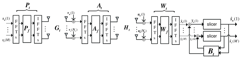
Figure 1: System model for a MIMO relay system with SC-FDE at the destination.

The remainder of this paper is organized as follows. In Section II, the system model is presented. In Section III, the optimal minimum MSE (MMSE) FDE filters and the corresponding stream error covariance (CV) matrices are derived. The optimal source and relay precoding matrices are presented in Section IV. Simulation results are given in Section V, and some conclusions are drawn in Section VI.

In this paper, $\rm tr({\mathbf{A}})$, ${\mathbf{A}}^{-1}$, ${\mathbf{A}}^{T}$, and ${\mathbf{A}}^{{\dagger}}$ denote the trace, inverse, transpose, and conjugate transpose of matrix ${\mathbf{A}}$, respectively. $\mathbb{C}^{M\times N}$ denotes the space of all $M\times N$ complex matrices and ${\mathbf{I}}_{M}$ is the $M\times M$ identity matrix. ${\mathbf{n}}\sim\mathcal{CN}(\mathbf{0},\sigma_{n}^{2}{\mathbf{I}}_{M})$ indicates that ${\mathbf{n}}\in\mathbb{C}^{M\times 1}$ is a complex Gaussian distributed vector with zero mean and CV matrix $\sigma_{n}^{2}{\mathbf{I}}_{M}$. $E[\cdot]$ and $\otimes$ denote statistical expectation and the Kronecker product, respectively. $\mbox{blkcirc}([{\mathbf{A}}_{1}^{T},{\mathbf{A}}_{2}^{T},...,{\mathbf{A}}_{M}^{T}]^{T})$ and $\mbox{blkdiag}([{\mathbf{A}}_{1}^{T},{\mathbf{A}}_{2}^{T},...,{\mathbf{A}}_{M}^{T}]^{T})$ denote a block circular matrix and a block diagonal matrix, respectively, formed by the block-wise vector $[{\mathbf{A}}_{1}^{T},{\mathbf{A}}_{2}^{T},...,{\mathbf{A}}_{M}^{T}]^{T}$. $\mathbb{F}_{N}$ denotes the $N\times N$ Discrete Fourier Transform (DFT) matrix, and $x^{\star}$ denotes the optimal value of $x$.

II System Model

We consider a block transmission system with one source node, $S$, one relay node, $R$, and one destination node, $D$, as shown in Fig. 1. The numbers of antennas at $S$, $R$, and $D$ are denoted by $N_{s}$, $N_{r}$, and $N_{d}$, respectively. The number of spatial multiplexing data streams is $M\leq\min\{N_{s},N_{r},N_{d}\}$. The transmission is organized in two phases. In the first phase, $S$ processes the information symbols and sends them to $R$. In the second phase, $R$ processes the received signal and retransmits it to $D$. We assume there is no direct link between $S$ and $D$ due to the large pathloss and/or shadowing.

The transmit signal of each source antenna is prepended by a cyclic prefix (CP), which comprises the last $N_{g,s}\geq L_{g}$ symbols of the transmitted source signal, where $L_{g}$ denotes the largest channel impulse response (CIR) length between any $S$-$R$ antenna pair. Similarly, the transmit signal of each relay antenna is prepended by a CP, which comprises the last $N_{g,r}\geq L_{h}$ symbols of the transmitted relay signal, where $L_{h}$ is the largest CIR length between any $R$-$D$ antenna pair.

II-A Precoding at Source and Relay

Let us denote the $n$th source data symbol vector as ${\mathbf{s}}_{n}=[s_{n}(1),s_{n}(2),\ldots,s_{n}(M)]^{T}$, $n=0,\ldots,N_{c}-1$, where $N_{c}$ is the size of the data block, and $s_{n}(j)$ denotes the $n$th symbol of the $j$th data stream, which is drawn from a constellation with variance $\sigma_{s}^{2}$. By stacking all ${\mathbf{s}}_{n}$ into one vector, we obtain ${\mathbf{s}}=[{\mathbf{s}}_{0}^{T},\ldots,{\mathbf{s}}_{N_{c}-1}^{T}]^{T}\in\mathbb{C}^{MN_{c}\times 1}$. The received signal at the destination, ${\mathbf{y}}$, can be compactly written as

$${\mathbf{y}}={\mathbf{H}}_{t}{\mathbf{A}}_{t}{\mathbf{G}}_{t}{\mathbf{P}}_{t}{\mathbf{s}}+{\mathbf{H}}_{t}{\mathbf{A}}_{t}{\mathbf{v}}+{\mathbf{u}}$$ (1)

with block circular matrices

$${\mathbf{P}}_{t} ={\rm blkcirc}([{\mathbf{P}}_{t,0}^{T},\cdots,{\mathbf{P}}_{t,N_{c}-1}^{T}]^{T}),$$

$${\mathbf{G}}_{t} ={\rm blkcirc}([{\mathbf{G}}_{t,0}^{T},\cdots,{\mathbf{G}}_{t,L_{g}-1}^{T},\mathbf{0}_{N_{s}\times N_{r}(N_{c}-L_{g})}]^{T}),$$

$${\mathbf{A}}_{t} ={\rm blkcirc}([{\mathbf{A}}_{t,0}^{T},\cdots,{\mathbf{A}}_{t,N_{c}-1}^{T}]^{T}),$$

$${\mathbf{H}}_{t} ={\rm blkcirc}([{\mathbf{H}}_{t,0}^{T},\cdots,{\mathbf{H}}_{t,L_{h}-1}^{T},\mathbf{0}_{N_{r}\times N_{d}(N_{c}-L_{h})}]^{T}),$$

where ${\mathbf{P}}_{t,l}\in\mathbb{C}^{N_{s}\times M}$, ${\mathbf{G}}_{t,l}\in\mathbb{C}^{N_{r}\times N_{s}}$, ${\mathbf{A}}_{t,l}\in\mathbb{C}^{N_{r}\times N_{r}}$, and ${\mathbf{H}}_{t,l}\in\mathbb{C}^{N_{d}\times N_{r}}$ denote the $l$th tap of the time-domain (TD) source precoding filter, the $S$-$R$ channel, the TD relay precoding filter, and the $R$-$D$ channel, respectively. The noise vectors at $R$ and $D$ are denoted by

$${\mathbf{v}} =[{\mathbf{v}}_{0}^{T},\ldots,{\mathbf{v}}_{N_{c}-1}^{T}]^{T}\sim\mathcal{CN}(\mathbf{0},\sigma_{v}^{2}{\mathbf{I}}_{N_{r}N_{c}}),$$

$${\mathbf{u}} =[{\mathbf{u}}_{0}^{T},\ldots,{\mathbf{u}}_{N_{c}-1}^{T}]^{T}\sim\mathcal{CN}(\mathbf{0},\sigma_{u}^{2}{\mathbf{I}}_{N_{d}N_{c}}),$$ (2)

where ${\mathbf{v}}_{n}=[v_{n}(1),v_{n}(2),\ldots,v_{n}(N_{r})]^{T}$ and ${\mathbf{u}}_{n}=[u_{n}(1),u_{n}(2),\ldots,u_{n}(N_{d})]^{T}$ denote the additive white Gaussian noise (AWGN) vectors at $R$ and $D$ at time $n$, respectively. The block circular matrices {${\mathbf{P}}_{t}$, ${\mathbf{G}}_{t}$, ${\mathbf{A}}_{t}$, ${\mathbf{H}}_{t}$} can be decomposed as

$${\mathbf{P}}_{t} ={\mathbf{F}}_{N_{s}}^{\dagger}{\mathbf{P}}_{f}{\mathbf{F}}_{M},\quad{\mathbf{G}}_{t}={\mathbf{F}}_{N_{r}}^{\dagger}{\mathbf{G}}_{f}{\mathbf{F}}_{N_{s}},$$

$${\mathbf{A}}_{t} ={\mathbf{F}}_{N_{r}}^{\dagger}{\mathbf{A}}_{f}{\mathbf{F}}_{N_{r}},\quad{\mathbf{H}}_{t}={\mathbf{F}}_{N_{d}}^{\dagger}{\mathbf{H}}_{f}{\mathbf{F}}_{N_{r}},\quad$$ (3)

with ${\mathbf{F}}_{\Upsilon}=\mathbb{F}_{N_{c}}^{\dagger}\otimes{\mathbf{I}}_{\Upsilon}$, $\Upsilon\in\{M,N_{s},N_{r},N_{d}\}$, ${\mathbf{X}}_{f}={\rm blkdiag}([{\mathbf{X}}_{0}^{T},\cdots,{\mathbf{X}}_{N_{c}-1}^{T}]^{T})$, and ${\mathbf{X}}_{f}\in\{{\mathbf{P}}_{f},{\mathbf{G}}_{f},{\mathbf{A}}_{f},{\mathbf{H}}_{f}\}$. Here, ${\mathbf{P}}_{k}\in\mathbb{C}^{N_{s}\times M}$, ${\mathbf{G}}_{k}\in\mathbb{C}^{N_{r}\times N_{s}}$, ${\mathbf{A}}_{k}\in\mathbb{C}^{N_{r}\times N_{r}}$, and ${\mathbf{H}}_{k}\in\mathbb{C}^{N_{d}\times N_{r}}$ represent the frequency-domain (FD) source precoding, $S$-$R$ channel, relay precoding, and $R$-$D$ channel matrices for the $k$th frequency tone, respectively. We define the equivalent end-to-end channel matrix ${\mathbf{Q}}_{t}={\mathbf{H}}_{t}{\mathbf{A}}_{t}{\mathbf{G}}_{t}{\mathbf{P}}_{t}$ and express it as ${\mathbf{Q}}_{t}={\mathbf{F}}_{N_{d}}^{\dagger}{\mathbf{Q}}_{f}{\mathbf{F}}_{M}$, where ${\mathbf{Q}}_{f}={\rm blkdiag}([{\mathbf{Q}}_{0}^{T},\cdots,{\mathbf{Q}}_{N_{c}-1}^{T}]^{T})$ with ${\mathbf{Q}}_{k}={\mathbf{H}}_{k}{\mathbf{A}}_{k}{\mathbf{G}}_{k}{\mathbf{P}}_{k}\in\mathbb{C}^{N_{d}\times M}$ representing the equivalent $S$-$D$ channel matrix on the $k$th frequency tone. Furthermore, the CV matrix of the equivalent noise vector ${\mathbf{n}}={\mathbf{H}}_{t}{\mathbf{A}}_{t}{\mathbf{v}}+{\mathbf{u}}$ can be obtained as

$${\mathbf{K}}=E[{\mathbf{n}}{\mathbf{n}}^{\dagger}]={\mathbf{F}}_{N_{d}}^{\dagger}{\mathbf{K}}_{f}{\mathbf{F}}_{N_{d}},$$ (4)

where ${\mathbf{K}}_{f}=\sigma_{v}^{2}{\mathbf{H}}_{f}{\mathbf{A}}_{f}{\mathbf{A}}_{f}^{\dagger}{\mathbf{H}}_{f}^{\dagger}+\sigma_{u}^{2}{\mathbf{I}}_{N_{d}N_{c}}$.

II-B Equalization at the Destination

The received signal ${\mathbf{y}}$ is transformed into the FD using ${\mathbf{F}}_{N_{d}}$ and equalized by an FD feedforward filter (FFF) ${\mathbf{W}}_{f}={\rm blkdiag}([{\mathbf{W}}_{0}^{T},\cdots,{\mathbf{W}}_{N_{c}-1}^{T}]^{T})$. The resulting signal is then transformed into the TD using ${\mathbf{F}}_{M}^{\dagger}$ resulting in

$$\hat{\mathbf{y}} = {\mathbf{W}}_{t}{\mathbf{y}},$$ (5)

where ${\mathbf{W}}_{t}={\mathbf{F}}_{M}^{\dagger}{\mathbf{W}}_{f}{\mathbf{F}}_{N_{d}}$ is the equivalent TD FFF and $\hat{\mathbf{y}}=[\hat{\mathbf{y}}_{0}^{T},\ldots,\hat{\mathbf{y}}_{N_{c}-1}^{T}]^{T}$ with $\hat{\mathbf{y}}_{n}=$$[\hat{y}_{n}(1),\hat{y}_{n}(2),\ldots,\hat{y}_{n}(M)]^{T}$ denoting the $n$th signal vector at the output of the FFF. If FD-LE is employed, $\hat{\mathbf{y}}_{n}$ is the decision variable for the $n$th source symbol vector. On the other hand, for FD-DFE, $\hat{\mathbf{y}}_{n}$ is further processed using a TD feedback filter (FBF) to perform interference cancelation. Assuming correct feedback at the output of the slicer, the signal corresponding to the $m$th data stream at time $n$ at the input of the slicer is given by

$$\bar{y}_{n}(m)=\hat{y}_{n}(m)-\sum_{l=0}^{N_{fb}}[{\mathbf{B}}_{t,l}]_{(m,:)}{\mathbf{s}}_{(n-l){{\rm mod}N_{c}}},$$ (6)

where ${\mathbf{B}}_{t,l}$ denotes the coefficient matrix of the $l$th tap of the FBF, $[{\mathbf{X}}]_{(m,:)}$ stands for the $m$th row of matrix ${\mathbf{X}}$, $N_{fb}$ is the number of feedback taps, and $(\cdot){\rm mod}N$ denotes the modulo-$N$ operation. From (6) we observe that at the initial stage of the feedback process, i.e., when $n=0$, $[{\mathbf{s}}_{N_{c}-N_{fb}},\cdots,{\mathbf{s}}_{N_{c}}]$ has to be known a priori, which can be accomplished by using known training symbols. Nevertheless, for detection of $s_{n}(m)$, $[s_{n}(1),\cdots,s_{n}(m-1)]$ is still unknown. Therefore, for causal detection, the $0$th tap of the FBF, i.e., ${\mathbf{B}}_{t,0}$, has to be a lower triangular matrix with zero diagonal entries. By collecting all $\bar{y}_{n}(m)$ into a vector $\bar{\mathbf{y}}=[\bar{\mathbf{y}}_{0}^{T},\ldots,\bar{\mathbf{y}}_{N_{c}-1}^{T}]^{T}$ with $\bar{\mathbf{y}}_{n}=[\bar{y}_{n}(1),\bar{y}_{n}(2),\ldots,\bar{y}_{n}(M)]^{T}$, we arrive at

$$\bar{\mathbf{y}}=\hat{\mathbf{y}}-{\mathbf{B}}_{t}{\mathbf{s}},$$ (7)

where ${\mathbf{B}}_{t}={\rm blkcirc}([{\mathbf{B}}_{t,0}^{T},\cdots,{\mathbf{B}}_{t,N_{fb}}^{T},\mathbf{0}_{M\times M(N_{c}-N_{fb}-1)}]^{T})\in\mathbb{C}^{MN_{c}\times MN_{c}}$ is the equivalent TD-FBF. Thus, the error vector at the input of the slicer can be expressed as

$${\mathbf{e}}=\bar{\mathbf{y}}-{\mathbf{s}}=\hat{\mathbf{y}}-\underbrace{({\mathbf{B}}_{t}+{\mathbf{I}}_{MN_{c}})}_{{\mathbf{C}}_{t}}{\mathbf{s}}=\hat{\mathbf{y}}-{\mathbf{C}}_{t}{\mathbf{s}},$$ (8)

where ${\mathbf{C}}_{t}={\rm blkcirc}([{\mathbf{C}}_{t,0}^{T},\cdots,{\mathbf{C}}_{t,N_{fb}}^{T},\mathbf{0}^{T}]^{T})$ with ${\mathbf{C}}_{t,n}={\mathbf{B}}_{t,n},\forall n\neq 0$ and ${\mathbf{C}}_{t,0}={\mathbf{B}}_{t,0}+{\mathbf{I}}_{M}$. The block circular matrix ${\mathbf{C}}_{t}$ can be decomposed as ${\mathbf{C}}_{t}={\mathbf{F}}_{M}^{\dagger}{\mathbf{C}}_{f}{\mathbf{F}}_{M}$, where ${\mathbf{C}}_{f}={\rm blkdiag}([{\mathbf{C}}_{0}^{T},\cdots,$ ${\mathbf{C}}_{N_{c}-1}^{T}]^{T})$. We note that by setting ${\mathbf{C}}_{t}={\mathbf{I}}_{MN_{c}}$, FD-DFE reduces to FD-LE.

III Optimal Minimum MSE FDE Filter Design

In this section, we derive the optimal minimum MSE equalization filters at the destination and the corresponding error CV matrices at the output of the equalizer as functions of the source and relay precoding matrices. Combining (1)-(5) and (8), the error CV matrix, ${\mathbf{E}}\triangleq E[{\mathbf{e}}{\mathbf{e}}^{\dagger}]$, can be expressed as

$${\mathbf{E}} = {\mathbf{F}}_{M}^{\dagger}\Big{(}{\mathbf{W}}_{f}(\sigma_{s}^{2}{\mathbf{Q}}_{f}{\mathbf{Q}}_{f}^{\dagger}+{\mathbf{K}}_{f}){\mathbf{W}}_{f}^{\dagger}-\sigma_{s}^{2}{\mathbf{W}}_{f}{\mathbf{Q}}_{f}{\mathbf{C}}_{f}^{\dagger}$$ (9)

$$-\sigma_{s}^{2}{\mathbf{C}}_{f}{\mathbf{Q}}_{f}^{\dagger}{\mathbf{W}}_{f}^{\dagger}+\sigma_{s}^{2}{\mathbf{C}}_{f}{\mathbf{C}}_{f}^{\dagger}\Big{)}{\mathbf{F}}_{M}.$$

Following the conventional equalization design methodology, the optimum FD FFF is obtained by minimizing the sum of stream MSEs, ${\rm tr}({\mathbf{E}})$, which yields

$${\mathbf{W}}_{f}^{\star}=\sigma_{s}^{2}{\mathbf{C}}_{f}{\mathbf{Q}}_{f}^{\dagger}\left(\sigma_{s}^{2}{\mathbf{Q}}_{f}{\mathbf{Q}}_{f}^{\dagger}+{\mathbf{K}}_{f}\right)^{-1}.$$ (10)

Substituting ${\mathbf{W}}_{f}^{\star}$ into (9) and simplifying the resulting expression, the CV matrix can be rewritten as

$${\mathbf{E}}=\sigma_{s}^{2}{\mathbf{F}}_{M}^{\dagger}{\mathbf{C}}_{f}\mathbf{\Psi}_{f}^{-1}{\mathbf{C}}_{f}^{\dagger}{\mathbf{F}}_{M},$$ (11)

where $\mathbf{\Psi}_{f}={\rm blkdiag}([\mathbf{\Psi}_{0}^{T},\cdots,\mathbf{\Psi}_{N_{c}-1}^{T}]^{T})\in\mathbb{C}^{MN_{c}\times MN_{c}}$ with

$$\mathbf{\Psi}_{k} =\sigma_{s}^{2}{\mathbf{Q}}_{k}^{\dagger}\left(\sigma_{v}^{2}{\mathbf{H}}_{k}{\mathbf{A}}_{k}{\mathbf{A}}_{k}^{\dagger}{\mathbf{H}}_{k}^{\dagger}+\sigma_{u}^{2}{\mathbf{I}}_{N_{d}}\right)^{-1}{\mathbf{Q}}_{k}+{\mathbf{I}}_{M}.$$ (12)

From (11) we observe that ${\mathbf{E}}$ is a block circular matrix. Hence, its block diagonal entries, ${\mathbf{E}}_{n}\in\mathbb{C}^{M\times M},\forall n$, are identical, i.e., ${\mathbf{E}}_{n}=\hat{\mathbf{E}},\forall n$. Since the diagonal entries of ${\mathbf{E}}_{n}$ represent the MSEs of the different spatial streams at time $n$, symbols from the same stream experience identical MSEs. CV matrix $\hat{\mathbf{E}}$ can be conveniently written as

$$\hat{\mathbf{E}}=\frac{\sigma_{s}^{2}}{N_{c}}\sum_{k=1}^{N_{c}}{\mathbf{C}}_{k}^{\dagger}\mathbf{\Psi}_{k}^{-1}{\mathbf{C}}_{k}.$$ (13)

III-A CV Matrix and Filter Design for FD-LE

Eqs. (10) and (13) are valid for both FD-LE and FD-DFE. For the special case of FD-LE, we can set ${\mathbf{C}}_{f}={\mathbf{I}}_{MN_{c}}$, which leads to

$${\mathbf{W}}_{f}^{\star}=\sigma_{s}^{2}{\mathbf{Q}}_{f}^{\dagger}\left(\sigma_{s}^{2}{\mathbf{Q}}_{f}{\mathbf{Q}}_{f}^{\dagger}+{\mathbf{K}}_{f}\right)^{-1}$$ (14)

and CV matrix

$$\hat{\mathbf{E}}_{\rm FD-LE}=\frac{\sigma_{s}^{2}}{N_{c}}\sum_{k=1}^{N_{c}}\mathbf{\Psi}_{k}^{-1}.$$ (15)

Interestingly, $\hat{\mathbf{E}}_{\rm FD-LE}$ is equal to the arithmetic mean of the subcarrier CV matrices, $\mathbf{\Psi}_{k}^{-1}$, in MIMO-OFDM relay systems [6].

III-B CV Matrix and Filter Design for FD-DFE

The FD-DFE CV matrix depends on the FD-FBF matrices ${\mathbf{C}}_{k}$. Since the FBF has to be implemented in the TD, we express ${\mathbf{C}}_{k}$ in terms of the TD FBF coefficients ${\mathbf{C}}_{t,n}$ as ${\mathbf{C}}_{k}=\sum_{n=0}^{N_{fb}}{\mathbf{C}}_{t,n}e^{-j\frac{2\pi}{N_{c}}nk}$. Now, (13) can be rewritten as

$$\hat{\mathbf{E}}_{\rm FD-DFE}$$ (16)

$$= \frac{\sigma_{s}^{2}}{N_{c}}\sum_{k=0}^{N_{c}-1}\Big{[}\sum_{n=0}^{N_{fb}}{\mathbf{C}}_{t,n}e^{-j\frac{2\pi}{N_{c}}nk}\mathbf{\Psi}_{k}^{-1}\sum_{m=0}^{N_{fb}}{\mathbf{C}}_{t,m}^{\dagger}e^{-j\frac{2\pi}{N_{c}}mk}\Big{]}$$

$$= \frac{\sigma_{s}^{2}}{N_{c}}\sum_{n=0}^{N_{fb}}\sum_{m=0}^{N_{fb}}\left({\mathbf{C}}_{t,n}\sum_{k=0}^{N_{c}-1}\mathbf{\Psi}_{k}^{-1}e^{-j\frac{2\pi}{N_{c}}(n-m)k}{\mathbf{C}}_{t,m}^{\dagger}\right)$$

$$= \frac{\sigma_{s}^{2}}{N_{c}}\hat{\mathbf{C}}{\mathbf{Z}}\hat{\mathbf{C}}^{\dagger}.$$

To simplify the notation, we have used the definitions $\hat{\mathbf{C}}=[{\mathbf{C}}_{t,0},...,{\mathbf{C}}_{t,N_{fb}}]$ and

$${\mathbf{Z}}=\left[\begin{array}[]{cccc}{\mathbf{z}}_{0}&{\mathbf{z}}_{1}&\ldots&{\mathbf{z}}_{N_{fb}}\\ {\mathbf{z}}_{1}^{\dagger}&{\mathbf{z}}_{0}&\ldots&{\mathbf{z}}_{N_{fb}-1}\\ \vdots&&\ddots&\vdots\\ {\mathbf{z}}_{N_{fb}}^{\dagger}&{\mathbf{z}}_{N_{fb}-1}^{\dagger}&\ldots&{\mathbf{z}}_{0}\\ \end{array}\right],$$ (21)

where ${\mathbf{z}}_{n}=\sum_{k=0}^{N_{c}-1}\mathbf{\Psi}_{k}^{-1}e^{j\frac{2\pi}{N_{c}}kn}$. The optimal $\hat{\mathbf{C}}$ minimizing ${\rm tr}\{{\mathbf{E}}_{\rm FD-DFE}\}$ can be obtained by solving

$$\min_{\hat{\mathbf{C}}\mathbf{\Theta}={\mathbf{C}}_{t,0}} {\rm tr}(\hat{\mathbf{C}}{\mathbf{Z}}\hat{\mathbf{C}}^{\dagger}),$$ (22)

where $\mathbf{\Theta}=[{\mathbf{I}}_{M},\mathbf{0}_{M\times(N_{fb}-1)}]$. Problem (22) can be solved using the standard Lagrange multiplier method, leading to [13]

$$\hat{\mathbf{C}}^{\star}={\mathbf{C}}_{t,0}(\mathbf{\Theta}{\mathbf{Z}}^{-1}\mathbf{\Theta})^{-1}\mathbf{\Theta}^{\dagger}{\mathbf{Z}}^{-1}.$$ (23)

By partitioning ${\mathbf{Z}}$ and ${\mathbf{Z}}^{-1}$ as

$${\mathbf{Z}}=\left[\begin{array}[]{cc}{\mathbf{Z}}_{11}&{\mathbf{Z}}_{12}\\ {\mathbf{Z}}_{12}^{\dagger}&{\mathbf{Z}}_{22}\\ \end{array}\right],{\mathbf{Z}}^{-1}=\left[\begin{array}[]{cc}{\mathbf{U}}_{11}&{\mathbf{U}}_{12}\\ {\mathbf{U}}_{12}^{\dagger}&{\mathbf{U}}_{22}\\ \end{array}\right],$$ (28)

where $\{{\mathbf{Z}}_{11},{\mathbf{U}}_{11}\}\in\mathbb{C}^{M\times M}$, $\{{\mathbf{Z}}_{12},{\mathbf{U}}_{12}\}\in\mathbb{C}^{M\times MN_{fb}}$, and $\{{\mathbf{Z}}_{22},{\mathbf{U}}_{22}\}\in\mathbb{C}^{MN_{fb}\times MN_{fb}}$, $\hat{\mathbf{C}}$ can be further expressed as

$$\hat{\mathbf{C}}=[{\mathbf{C}}_{t,0}^{-1},\quad{\mathbf{C}}_{t,0}^{-1}{\mathbf{Z}}_{12}{\mathbf{Z}}_{22}^{-1}].$$ (29)

Substituting (29) into (16), the FD-DFE CV matrix can be rewritten as

$${\mathbf{E}}_{\rm FD-DFE}=\frac{\sigma_{s}^{2}}{N_{c}}{\mathbf{C}}_{t,0}{\mathbf{U}}_{11}^{-1}{\mathbf{C}}_{t,0}^{\dagger}.$$ (30)

To complete the FBF design, the optimal ${\mathbf{C}}_{t,0}$ has to be determined. To this end, we introduce the Cholesky decomposition of ${\mathbf{U}}_{11}^{-1}$ as

$${\mathbf{U}}_{11}^{-1}={\mathbf{L}}{\mathbf{D}}{\mathbf{L}}^{\dagger},$$ (31)

where ${\mathbf{L}}$ is a unit-diagonal lower triangular matrix and ${\mathbf{D}}$ is a diagonal matrix with positive main diagonal entries. Now, it is easy to verify that the optimal ${\mathbf{C}}_{t,0}$ which minimizes ${\rm tr}({\mathbf{E}}_{\rm FD-DFE})$ is given by ${\mathbf{C}}_{t,0}^{\star}={\mathbf{L}}^{-1}$. Hence, the optimal $\hat{\mathbf{C}}$ is obtained as

$$\hat{\mathbf{C}}^{\star}=[{\mathbf{L}}^{-1},\quad{\mathbf{L}}^{-1}{\mathbf{Z}}_{12}{\mathbf{Z}}_{22}^{-1}].$$ (32)

The structure of the optimal FBF can be interpreted as follows: ${\mathbf{L}}^{-1}\in\mathbb{C}^{M\times M}$ is a lower-triangular matrix which cancels the inter-antenna interference (IAI) in the current time slot, and the remaining FBF coefficients, ${\mathbf{L}}^{-1}{\mathbf{Z}}_{12}{\mathbf{Z}}_{22}^{-1}\in\mathbb{C}^{M\times MN_{fb}}$, cancel both the IAI and inter-symbol interference (ISI) stemming from the previous $N_{fb}-1$ time slots. Inserting $\hat{\mathbf{C}}^{\star}$ into (30) the error CV matrix can be written as

$$\hat{\mathbf{E}}_{\rm FD-DFE}=\frac{\sigma_{s}^{2}}{N_{c}}{\mathbf{D}}.$$ (33)

Interestingly, unlike for FD-LE, the error CV matrix for FD-DFE is a diagonal matrix, which also depends on the number of FBF taps $N_{fb}$.

IV Source and Relay Precoding Matrix Optimization

Exploiting the expressions for the error CV matrix obtained in the previous section, in this section, we minimize a general function $f(\mbox{diag}[\hat{\mathbf{E}}])$ of the spatial stream MSEs at the output of the equalization filter under separate constraints on the powers consumed at the source and the relay. Mathematically, the optimization problem is stated as

$$\min_{\{{\mathbf{P}}_{k},{\mathbf{A}}_{k}\}} f(\mbox{diag}[\hat{\mathbf{E}}])$$

s.t. $${\rm tr}\left(E[{\mathbf{x}}{\mathbf{x}}^{\dagger}]\right)\leq P_{S},\quad{\rm tr}\left(E[{\mathbf{t}}{\mathbf{t}}^{\dagger}]\right)\leq P_{R},$$ (34)

where $\hat{\mathbf{E}}=\hat{\mathbf{E}}_{\rm FD-LE}$ and $\hat{\mathbf{E}}=\hat{\mathbf{E}}_{\rm FD-DFE}$ for FD-LE and FD-DFE, respectively, $P_{S}$ and $P_{R}$ are the power budgets for $S$ and $R$, respectively, and $\mbox{diag}[{\mathbf{M}}]$ denotes a vector containing the main diagonal entries of matrix ${\mathbf{M}}$. The objective function $f(\mbox{diag}[\hat{\mathbf{E}}])$ can be either a Schur-convex or a Schur-concave increasing function with respect to (w.r.t.) $\mbox{diag}[\hat{\mathbf{E}}]$ [14]. For concreteness, in this paper, we consider the three most important objective functions of this type, namely the arithmetic MSE (AMSE), the geometric MSE (GMSE), and the maximum MSE (maxMSE)

$$f(\mbox{diag}[\hat{\mathbf{E}}])=\begin{cases}\begin{array}[]{c}\sum_{m=1}^{M}\hat{\mathbf{E}}_{mm},\quad\mbox{AMSE}\\ \prod_{m=1}^{M}\hat{\mathbf{E}}_{mm},\quad\mbox{GMSE}\\ \max_{m=1}^{M}\hat{\mathbf{E}}_{mm},\quad\mbox{maxMSE}\\ \end{array}\end{cases},$$ (35)

where $\hat{\mathbf{E}}_{mm}$ denotes the $m$th diagonal entry of $\hat{\mathbf{E}}$. The AMSE and GMSE are Schur-concave functions while the maxMSE is a Schur-convex function w.r.t. $\mbox{diag}[\hat{\mathbf{E}}]$ [14]. We note that similar objective functions have been considered for MIMO-OFDM based relay systems in [6]. However, for MIMO-OFDM based relay systems, the AMSE, GMSE, and maxMSE are the sum, product, and maximum of the subcarrier MSEs of different spatial sub-streams. In contrast, in (35), these three quantities are the the sum, product, and maximum of the sub-stream MSEs of a single carrier.

The power consumptions at source and relay are given by

$${\rm tr}\left(E[{\mathbf{x}}{\mathbf{x}}^{\dagger}]\right) =\sigma_{s}^{2}\sum_{k=0}^{N_{c}-1}{\rm tr}\left({\mathbf{P}}_{k}{\mathbf{P}}_{k}^{\dagger}\right),$$

$${\rm tr}\left(E[{\mathbf{t}}{\mathbf{t}}^{\dagger}]\right) =\sum_{k=0}^{N_{c}-1}{\rm tr}\left({\mathbf{A}}_{k}\left(\sigma_{s}^{2}{\mathbf{G}}_{k}{\mathbf{P}}_{k}{\mathbf{P}}_{k}^{\dagger}{\mathbf{G}}_{k}^{\dagger}+\sigma_{v}^{2}{\mathbf{I}}_{N_{r}}\right){\mathbf{A}}_{k}^{\dagger}\right).$$ (36)

Since the optimization variables in (34) are matrices, solving the problem directly would incur high complexity. In the following, we will first derive the structure of the optimal precoding matrices. Knowing this structure will allow us to transform the optimization problem into an optimization problem with scalar variables.

IV-A Structure of the Optimal Precoding Matrices for FD-LE

We first derive the structure of the optimal source and relay precoding matrices for FD-LE. We begin by introducing the following singular-value decompositions (SVDs) of the channel matrices

$${\mathbf{G}}_{k} ={\mathbf{U}}_{G}^{(k)}\mathbf{\Lambda}_{G}^{(k)}{\mathbf{V}}_{G}^{(k){\dagger}},\quad{\mathbf{H}}_{k}={\mathbf{U}}_{H}^{(k)}\mathbf{\Lambda}_{H}^{(k)}{\mathbf{V}}_{H}^{(k){\dagger}},\quad\forall k,$$ (37)

where ${\mathbf{U}}_{G}^{(k)}\in\mathbb{C}^{N_{r}\times N_{r}}$, ${\mathbf{V}}_{G}^{(k)}\in\mathbb{C}^{N_{s}\times N_{s}}$ and ${\mathbf{U}}_{H}^{(k)}\in\mathbb{C}^{N_{d}\times N_{d}}$, ${\mathbf{V}}_{H}^{(k)}\in\mathbb{C}^{N_{r}\times N_{r}}$ are the singular-vector matrices of ${\mathbf{G}}_{k}$ and ${\mathbf{H}}_{k}$, respectively. Furthermore, $\mathbf{\Lambda}_{G}^{(k)}\in\mathbb{C}^{N_{r}\times N_{s}}$ and $\mathbf{\Lambda}_{H}^{(k)}\in\mathbb{C}^{N_{d}\times N_{r}}$ are the singular-value matrices of ${\mathbf{G}}_{k}$ and ${\mathbf{H}}_{k}$, respectively, and have both increasing main diagonal elements.

Theorem 1

For the optimization problem in (34), the following structures of ${\mathbf{P}}_{k}$ and ${\mathbf{A}}_{k}$ are optimal

$${\mathbf{P}}_{k}^{\star} =\bar{{\mathbf{V}}}_{G}^{(k)}\mathbf{\Lambda}_{P}^{(k)}{\mathbf{V}}_{0},\quad{\mathbf{A}}_{k}^{\star}=\bar{{\mathbf{V}}}_{H}^{(k)}\mathbf{\Lambda}_{A}^{(k)}\bar{{\mathbf{U}}}_{G}^{(k)},\quad\forall k,$$ (38)

where $\bar{{\mathbf{V}}}_{G}^{(k)}$, $\bar{{\mathbf{U}}}_{G}^{(k)}$, and $\bar{{\mathbf{V}}}_{H}^{(k)}$ contain the $M$ right-most columns of ${{\mathbf{V}}}_{G}^{(k)}$, ${{\mathbf{U}}}_{G}^{(k)}$, and ${{\mathbf{V}}}_{H}^{(k)}$, respectively. $\mathbf{\Lambda}_{P}^{(k)}$ and $\mathbf{\Lambda}_{A}^{(k)}$ are $M\times M$ diagonal matrices with the $m$th diagonal element denoted by $p_{km}$ and $a_{km}$, respectively. For Schur-concave functions, ${\mathbf{V}}_{0}={\mathbf{I}}_{M}$. For Schur-convex functions, ${\mathbf{V}}_{0}$ is a unitary matrix chosen in such a way that all main diagonal entries of $\hat{\mathbf{E}}$ are equal.

Proof:

Please refer to the Appendix. ∎

Theorem 1 implies that for Schur-concave functions, the source and relay precoding matrices jointly diagonalize the MIMO relay channels at each frequency tone, while for Schur-convex functions, the precoding matrices diagonalize the channels up to a unitary rotation at the source. Therefore, the original optimization problem involving matrix variables can be transformed into a scalar power optimization problem across different spatial beams and frequency tones.

IV-B Transformation of Optimization Problem for FD-LE

Since the maxMSE is a Schur-convex function, according to Theorem 1, the unitary matrix, ${\mathbf{V}}_{0}$, should be chosen to make all diagonal entries of $\hat{\mathbf{E}}$ equal. Recall from Section III that $\mbox{diag}[\hat{\mathbf{E}}]$ represents the MSE of different spatial streams and all symbols of a particular stream have the same MSE. This means that for maxMSE, identical MSE is achieved for all symbols in the SC-FDE system. Hence, the remaining maxMSE power allocation problem is identical to that for the AMSE criterion. The only difference between the solutions for maxMSE and AMSE minimization lies in the choice of ${\mathbf{V}}_{0}$. We note that this is not true for MIMO-OFDM relay systems, where the unitary transformation at the source only achieves identical spatial MSEs on each subcarrier, while the MSEs across subcarriers are in general different. To balance these MSEs, multilevel waterfilling has to be carried out in such MIMO-OFDM relay systems, which entails a much higher complexity compared to the single-level waterfilling required for the AMSE criterion, cf. [6]. Additionally, for MIMO-OFDM relay systems, the unitary rotation matrices are in general different on each subcarrier as the number of transmitted data streams may vary from subcarrier to subcarrier. However, for SC-FDE, the rotation matrices are identical for all frequency tones since the number of data streams is determined in the time domain.

Because of the equivalence of the power allocation problems for maxMSE and AMSE, in the following, we focus on the power allocation problem for the AMSE and GMSE criteria. From (12) and (38), we obtain $\mathbf{\Psi}_{k}={\mathbf{V}}_{0}^{{\dagger}}\mathbf{\Phi}_{k}{\mathbf{V}}_{0}$ with

$$\mathbf{\Phi}_{k} = \sigma_{s}^{2}\mathbf{\Lambda}_{P}^{(k)2}\bar{\mathbf{\Lambda}}_{G}^{(k)2}\mathbf{\Lambda}_{A}^{(k)2}\bar{\mathbf{\Lambda}}_{H}^{(k)2}$$ (39)

$$\left(\sigma_{v}^{2}\mathbf{\Lambda}_{A}^{(k)2}\bar{\mathbf{\Lambda}}_{H}^{(k)2}+\sigma_{u}^{2}{\mathbf{I}}_{M}\right)^{-1}+{\mathbf{I}}_{M},$$

where $\bar{\mathbf{\Lambda}}_{G}^{(k)}$ and $\bar{\mathbf{\Lambda}}_{H}^{(k)}$ are diagonal matrices whose diagonal entries contain the $M$ largest singular values of ${{\mathbf{G}}}^{(k)}$ and ${{\mathbf{H}}}^{(k)}$, respectively. Now, we can rewrite the objective functions as

$$f_{\rm X}(\mathbf{\Phi})=\begin{cases}\begin{array}[]{c}\sum_{m=1}^{M}\left(\frac{1}{N_{c}}\sum_{k=0}^{N_{c}-1}{\Phi}_{km}^{-1}\right),\mbox{ X=AMSE}\\ \sum_{m=1}^{M}\log_{2}\left(\frac{1}{N_{c}}\sum_{k=0}^{N_{c}-1}{\Phi}_{km}^{-1}\right),\mbox{ X=GMSE}\end{array}\end{cases},$$ (40)

where $\mathbf{\Phi}=\{{\Phi}_{km},\forall k,m\}$ with

$${\Phi}_{km}=\frac{\sigma_{s}^{2}p_{km}^{2}g_{km}^{2}a_{km}^{2}h_{km}^{2}}{\sigma_{v}^{2}a_{km}^{2}h_{km}^{2}+\sigma_{u}^{2}}+1.$$ (41)

Here, $g_{km}$ and $h_{km}$ denote the $m$th main diagonal elements of $\bar{\mathbf{\Lambda}}_{G}^{(k)}$ and $\bar{\mathbf{\Lambda}}_{H}^{(k)}$, respectively, and represent the corresponding channel gains of the $m$th spatial stream on the $k$th frequency tone. Note that, for the GMSE criterion, we have taken the logarithm of the original objective function to facilitate the subsequent optimization. Due to the monotonicity of the logarithm, the new objective function has the same optimal solution as the original one. The new objective function can be rewritten as

$$-\sum_{m=1}^{M}\log_{2}\left({{\rm SINR}_{m}}+1\right),$$ (42)

where ${{\rm SINR}_{m}}=(\frac{1}{N_{c}}\sum_{k=0}^{N_{c}-1}{\Phi}_{km}^{-1})^{-1}-1$ is the signal-to-interference-plus-noise ratio (SINR) of the $m$th data stream. This implies that (42) is essentially the negative sum of the channel capacities of different spatial streams. Therefore, minimization of the GMSE is equivalent to the maximization of the capacity of the considered MIMO SC-FDE relay system. By exploiting (38), the expression for the power consumption on the left hand side of the constraints in (34) can be expressed as

$${\rm tr}\left(E[{\mathbf{x}}{\mathbf{x}}^{\dagger}]\right) = \sigma_{s}^{2}\sum_{k=0}^{N_{c}-1}{\rm tr}\left(\mathbf{\Lambda}_{P}^{(k)2}\right)=\sum_{k=0}^{N_{c}-1}\sum_{m=1}^{M}P_{s,km}$$

$${\rm tr}\left(E[{\mathbf{t}}{\mathbf{t}}^{\dagger}]\right) = \sum_{k=0}^{N_{c}-1}{\rm tr}\left(\mathbf{\Lambda}_{A}^{(k)2}\left(\sigma_{s}^{2}\mathbf{\Lambda}_{P}^{(k)2}\bar{\mathbf{\Lambda}}_{G}^{(k)2}+\sigma_{u}^{2}{\mathbf{I}}_{M}\right)\right)$$ (43)

$$= \sum_{k=0}^{N_{c}-1}\sum_{m=1}^{M}P_{r,km},$$

where

$$P_{s,km}=\sigma_{s}^{2}p_{km}^{2},\quad P_{r,km}=a_{km}^{2}(\sigma_{s}^{2}p_{km}^{2}g_{km}^{2}+\sigma_{v}^{2})$$ (44)

can be interpreted as the power allocated to the $k$th frequency tone and the $m$th spatial stream at the source and the relay, respectively. By rewriting ${\Phi}_{km}$ in terms of the newly introduced variables $P_{s,km}$ and $P_{r,km}$ as

$${\Phi}_{km}=\frac{P_{s,km}P_{r,km}g_{km}^{2}h_{km}^{2}}{\sigma_{v}^{2}P_{r,km}h_{km}^{2}+\sigma_{u}^{2}(P_{s,km}g_{km}^{2}+\sigma_{v}^{2})}+1,$$ (45)

problem (34) can be reformulated as the following power allocation problem

$$\min_{\{P_{s.km},P_{r,km}\}} f_{\rm X}\left(\mathbf{\Phi}\right)$$

s.t. $$\sum_{k=0}^{N_{c}-1}\sum_{m=1}^{M}P_{s,km}\leq P_{S},$$ (46)

$$\sum_{k=0}^{N_{c}-1}\sum_{m=1}^{M}P_{r,km}\leq P_{R},$$

$$P_{s,km}\geq 0,P_{r,km}\geq 0,\forall k,m,$$

where the constraints $P_{s,km}\geq 0,P_{r,km}\geq 0,\forall k,m$, ensure that the allocated powers are not negative.

IV-C Structure of the Optimal Precoding Matrices for FD-DFE

For the FD-DFE receiver, we observe from (33) that ${\mathbf{E}}_{\rm FD-DFE}$ is not an explicit function of optimization variables ${\mathbf{P}}_{k}$ and ${\mathbf{A}}_{k}$, which renders the optimization a challenging task. In the following, we will show that by using some proper transformations, an upper bound for the original objective function can be derived, which is equivalent to one of the objective functions considered for the FD-LE receiver. However, first we will show that for FD-DFE, the three considered objective functions are equivalent.

IV-C1 Equivalence of Objective Functions

Since ${\mathbf{E}}_{\rm FD-DFE}$ in (33) is a diagonal matrix, we invoke the following matrix arithmetic-geometric mean inequality

$$\frac{1}{M}{\rm tr}({\mathbf{D}})=\frac{1}{M}\sum_{i=1}^{M}[{\mathbf{D}}]_{(i,i)}\geq(\prod_{i=1}^{M}[{\mathbf{D}}]_{(i,i)})^{\frac{1}{M}}=\det({\mathbf{D}})^{\frac{1}{M}},$$ (47)

where equality holds if and only if (i.f.f.) all main diagonal elements of ${\mathbf{D}}$ are equal. The inequality provides some important insights into the objective function for FD-DFE. First, it implies that the AMSE, i.e., ${\rm tr}({\mathbf{D}})$, is lower bounded by the term involving the GMSE, i.e., $\det({\mathbf{D}})$. Second, this lower bound is achieved i.f.f. the MSEs of all streams are identical. Therefore, making the diagonal entries of ${\mathbf{D}}$ identical will enable us to minimize the AMSE, GMSE, and maxMSE simultaneously. Consequently, for FD-DFE, the three considered objective functions become equivalent if this condition is fulfilled, and the value of the objective function is equal to $\det({\mathbf{D}})^{\frac{1}{M}}$. In the sequel, we will show how this can be achieved by properly choosing a unitary matrix at the source precoder. By noting that

$${\rm det}({\mathbf{D}})={\rm det}({\mathbf{L}}{\mathbf{D}}{\mathbf{L}}^{\dagger})={\rm det}({\mathbf{U}}_{11}^{-1}),$$ (48)

where we have exploited the properties that ${\rm det}({\mathbf{A}}{\mathbf{B}})={\rm det}({\mathbf{A}}){\rm det}({\mathbf{B}})$ and ${\rm det}({\mathbf{L}})=1$ [18], we can obtain

$${\mathbf{U}}_{11}^{-1} = {\mathbf{L}}{\mathbf{D}}^{1/2}({\mathbf{L}}{\mathbf{D}}^{1/2})^{\dagger}=({\mathbf{Q}}{\mathbf{R}})^{\dagger}{\mathbf{Q}}{\mathbf{R}},$$ (49)

where ${\mathbf{Q}}$ is an arbitrary unitary matrix of appropriate dimension and ${\mathbf{R}}=({\mathbf{L}}{\mathbf{D}}^{1/2})^{\dagger}$ is a lower triangular matrix whose main diagonal elements are equal to the square root of the main diagonal elements of ${\mathbf{D}}$. Therefore, finding a matrix ${\mathbf{D}}$ with equal diagonal elements is equivalent to finding a matrix ${\mathbf{R}}$ with equal diagonal elements. Since it follows from (49) that ${\mathbf{U}}_{11}^{-1/2}={\mathbf{Q}}{\mathbf{R}}$, we have to find a matrix decomposition of ${\mathbf{U}}_{11}^{-1/2}$ such that ${\mathbf{R}}$ has identical diagonal elements. Such a decomposition is referred to as equal-diagonal QR decomposition (E-QRD) [16] or geometric-mean decomposition (GMD) [17]. Note that for an arbitrary matrix $\mathbf{\Xi}$, the standard form of the GMD is,

$$\mathbf{\Xi}{\mathbf{V}}_{1}^{\dagger}={\mathbf{Q}}{\mathbf{R}},$$ (50)

where ${\mathbf{V}}_{1}$ is a unitary matrix chosen to make the diagonal entries of ${\mathbf{R}}$ all equal. Therefore, to facilitate the application of GMD, we rewrite ${\mathbf{U}}_{11}^{-1/2}$ as

$${\mathbf{U}}_{11}^{-1/2}=\mathbf{\Xi}{\mathbf{V}}_{1}^{\dagger}$$ (51)

In the following, we will find the explicit expression for $\mathbf{\Xi}$ to perform the decomposition in (50). By expressing ${\mathbf{P}}_{k}$ as the product of ${\mathbf{V}}_{1}$ and a general matrix $\tilde{\mathbf{P}}_{k}$,

$${\mathbf{P}}_{k} = \tilde{\mathbf{P}}_{k}{\mathbf{V}}_{1}^{{\dagger}},$$ (52)

we can write $\mathbf{\Psi}_{k}$ as $\mathbf{\Psi}_{k}={\mathbf{V}}_{1}\mathbf{\hat{\Psi}}_{k}{\mathbf{V}}_{1}^{\dagger}$, where

$$\mathbf{\hat{\Psi}}_{k} = \sigma_{s}^{2}\tilde{\mathbf{P}}_{k}^{\dagger}{\mathbf{G}}_{k}^{\dagger}{\mathbf{A}}_{k}^{\dagger}{\mathbf{H}}_{k}^{\dagger}\Big{(}\sigma_{v}^{2}{\mathbf{H}}_{k}{\mathbf{A}}_{k}{\mathbf{A}}_{k}^{\dagger}{\mathbf{H}}_{k}^{\dagger}+\sigma_{u}^{2}{\mathbf{I}}_{N_{d}}\Big{)}^{-1}$$ (53)

$${\mathbf{H}}_{k}{\mathbf{A}}_{k}{\mathbf{G}}_{k}\tilde{\mathbf{P}}_{k}+{\mathbf{I}}_{M}.$$

Note that $\mathbf{\hat{\Psi}}_{k}$ has the same form of ${\mathbf{\Psi}}_{k}$ in (12) but with ${\mathbf{P}}_{k}$ replaced by $\tilde{\mathbf{P}}_{k}$. Therefore, matrix ${\mathbf{Z}}$ in (21) can be written as

$${\mathbf{Z}} =\left[\begin{array}[]{cccc}{\mathbf{V}}_{1}\bar{\mathbf{z}}_{0}{\mathbf{V}}_{1}^{{\dagger}}&{\mathbf{V}}_{1}\bar{\mathbf{z}}_{1}{\mathbf{V}}_{1}^{{\dagger}}&\ldots&{\mathbf{V}}_{1}\bar{\mathbf{z}}_{N_{fb}}{\mathbf{V}}_{1}^{{\dagger}}\\ {\mathbf{V}}_{1}\bar{\mathbf{z}}_{1}^{\dagger}{\mathbf{V}}_{1}^{{\dagger}}&{\mathbf{V}}_{1}\bar{\mathbf{z}}_{0}{\mathbf{V}}_{1}^{{\dagger}}&\ldots&{\mathbf{V}}_{1}\bar{\mathbf{z}}_{N_{fb}-1}\\ \vdots&&\ddots&\vdots\\ {\mathbf{V}}_{1}\bar{\mathbf{z}}_{N_{fb}}^{\dagger}{\mathbf{V}}_{1}^{{\dagger}}&{\mathbf{V}}_{1}\bar{\mathbf{z}}_{N_{fb}-1}^{\dagger}{\mathbf{V}}_{1}^{{\dagger}}&\ldots&{\mathbf{V}}_{1}\bar{\mathbf{z}}_{0}{\mathbf{V}}_{1}^{{\dagger}}\\ \end{array}\right]$$ (58)

$$=({\mathbf{I}}_{N_{fb}}\otimes{\mathbf{V}}_{1})\bar{\mathbf{Z}}({\mathbf{I}}_{N_{fb}}\otimes{\mathbf{V}}_{1}^{\dagger}),$$ (59)

where $\bar{\mathbf{Z}}$ has the same form as ${\mathbf{Z}}$ in (21) with ${\mathbf{z}}_{n}$ replaced by $\bar{\mathbf{z}}_{n}={\sum_{k=0}^{N_{c}-1}\hat{\mathbf{\Psi}}_{k}^{-1}e^{j\frac{2\pi}{N_{c}}kn}}$. By noting that

$${\mathbf{Z}}^{-1}=({\mathbf{I}}_{N_{fb}}\otimes{\mathbf{V}}_{1})\bar{\mathbf{Z}}^{-1}({\mathbf{I}}_{N_{fb}}\otimes{\mathbf{V}}_{1}^{\dagger}),$$ (60)

where we have used $({\mathbf{I}}_{N_{fb}}\otimes{\mathbf{V}}_{1})^{-1}={\mathbf{I}}_{N_{fb}}\otimes{\mathbf{V}}_{1}^{{\dagger}}$, we obtain from (28)

$${\mathbf{U}}_{11}^{-1}={\mathbf{V}}_{1}\bar{\mathbf{U}}_{11}^{-1}{\mathbf{V}}_{1}^{\dagger},$$ (61)

where $\bar{\mathbf{U}}_{11}$ is the first $M\times M$ submatrix of $\bar{\mathbf{Z}}^{-1}$. Comparing (61) with (51), we observe that $\bar{\mathbf{U}}_{11}^{-1/2}$ is the explicit form for $\mathbf{\Xi}$. Hence, for a given $\bar{\mathbf{U}}_{11}$, we can always find a unitary matrix ${\mathbf{V}}_{1}$ which achieves the MSE lower bound.

As $\bar{\mathbf{U}}_{11}$ is a function of relay precoding matrix ${\mathbf{A}}_{k}$ as well as the remaining part of the source precoding matrix, i.e., $\tilde{\mathbf{P}}_{k}$, in the following, we need to determine these matrices. To this end, we write ${\mathbf{U}}_{11}=({\mathbf{Z}}_{11}-{\mathbf{Z}}_{12}^{\dagger}{\mathbf{Z}}_{22}^{-1}{\mathbf{Z}}_{12})^{-1}$ [18], which allows us to express the objective function for FD-DFE as

$$\mbox{OBJ}=\det({\mathbf{U}}_{11}^{-1})=\det\left({\mathbf{Z}}_{11}-{\mathbf{Z}}_{12}^{\dagger}{\mathbf{Z}}_{22}^{-1}{\mathbf{Z}}_{12}\right).$$ (62)

IV-C2 Upper Bound on Objective Function

Unfortunately, the expression for OBJ in (62) depends on the FBF length $N_{fb}$, cf. (59), which is not desirable in practice. Additionally, due to the presence of ${\mathbf{Z}}_{22}^{-1}$ in (62), it is also not straightforward to express the objective function in terms of ${\mathbf{A}}_{k}$ and $\tilde{\mathbf{P}}_{k}$. To avoid these problems, we derive an upper bound for OBJ, which is independent of $N_{fb}$ and directly related to the optimization variables.

Since matrix ${\mathbf{Z}}$ in (21) is a positive semidefinite (PSD) matrix, ${\mathbf{Z}}^{-1}$, ${\mathbf{Z}}_{22}$, and ${\mathbf{U}}_{11}$ are PSD matrices as well. Thus, ${\mathbf{U}}_{11}^{-1}$ and ${\mathbf{Z}}_{12}^{\dagger}{\mathbf{Z}}_{22}^{-1}{\mathbf{Z}}_{12}$ are also PSD matrices. By exploiting the fact that $\det\left({\mathbf{A}}+{\mathbf{B}}\right)\geq\det\left({\mathbf{A}}\right)$ if ${\mathbf{A}}$ and ${\mathbf{B}}$ are PSD matrices [18], we obtain

$$\det({\mathbf{U}}_{11}^{-1})\leq\det\left({\mathbf{Z}}_{11}\right),$$ (63)

where equality holds i.f.f. $N_{fb}=0$. Therefore, for the case of $N_{fb}=0$, $\det\left({\mathbf{Z}}_{11}\right)$ is the exact value of OBJ. Otherwise, it is an upper bound for OBJ, which can be expressed as

$$\mbox{OBJ}_{ub} ={\rm det}({\mathbf{Z}}_{11})={\rm det}\left(\sum_{k=1}^{N_{c}}\mathbf{\Psi}_{k}^{-1}\right)$$

$$={\rm det}\left(\sum_{k=1}^{N_{c}}{\mathbf{V}}_{1}\mathbf{\hat{\Psi}}_{k}^{-1}{\mathbf{V}}_{1}^{\dagger}\right)={\rm det}\left(\sum_{k=1}^{N_{c}}\mathbf{\hat{\Psi}}_{k}^{-1}\right),$$ (64)

where we exploited $\det({\mathbf{V}}_{1})=1$.

IV-C3 Structures of Optimal Source and Relay Precoding Matrices

Since we can always chose $\tilde{\mathbf{P}}_{k}$ such that $\sum_{k=1}^{N_{c}}\mathbf{\hat{\Psi}}_{k}^{-1}$ a diagonal matrix, cf. (53), the determinant in (64) is essentially the product of the diagonal entries of $\sum_{k=1}^{N_{c}}\mathbf{\hat{\Psi}}_{k}^{-1}$. Consequently, $\mbox{OBJ}_{ub}$ is equivalent to the objective function for the FD-LE receiver under the GMSE criterion. Thus, from Theorem 1 we obtain the following optimal structures for $\tilde{\mathbf{P}}_{k}$ and ${\mathbf{A}}_{k}$

$$\tilde{\mathbf{P}}_{k}^{\star}=\bar{\mathbf{V}}_{G}^{(k)}\mathbf{\Lambda}_{P}^{(k)},\quad{\mathbf{A}}_{k}^{\star}=\bar{\mathbf{V}}_{H}^{(k)}\mathbf{\Lambda}_{A}^{(k)}\bar{\mathbf{U}}_{G}^{(k){\dagger}}.$$ (65)

And the optimal ${\mathbf{P}}_{k}^{\star}$ is thus given by $\tilde{\mathbf{P}}_{k}^{\star}{\mathbf{V}}_{1}^{\dagger}$. The remaining power allocation problem is identical to that for the GMSE criterion for FD-LE, cf. (46). It is worth mentioning that for $N_{fb}>0$, the upper bound $\mbox{OBJ}_{ub}$ constitutes a tight approximation of the objective function OBJ as is illustrated in Section V.

IV-D Optimal Power Allocation

From the previous two subsections, it can be concluded that only two different types of power allocation problems have to be solved, namely the problems for the AMSE and GMSE criteria for FD-LE. The solutions to these problems are also applicable for the maxMSE criterion for FD-LE and all three criteria for FD-DFE. However, since the objective functions for the AMSE and GMSE criteria in (46) are not jointly convex w.r.t. the power allocation variables, the global optimal solution is difficult to obtain. Thus, in the following, we adopt a high signal-to-noise ratio (SNR) approximation for ${\Phi}_{km}$, i.e., we assume $\sigma_{u}^{2}\sigma_{v}^{2}$ is sufficient small such that it can be ignored in the denominator of (45), which leads to

$${\Phi}_{km}\approx{\tilde{\Phi}}_{km}=\frac{P_{s,km}P_{r,km}g_{km}^{2}h_{km}^{2}}{\sigma_{v}^{2}P_{r,km}h_{km}^{2}+\sigma_{u}^{2}P_{s,km}g_{km}^{2}}+1.$$ (66)

This approximation renders the optimization problem convex such that efficient methods can be applied for its solution. In particular, it can be shown that both objective functions $f_{\rm AMSE}(\tilde{\mathbf{\Phi}})$ and $f_{\rm GMSE}(\tilde{\mathbf{\Phi}})$, $\tilde{\mathbf{\Phi}}=\{\tilde{\Phi}_{km}$ , $\forall k,m\}$, are jointly convex w.r.t. the power allocation variables $P_{s,km}$ and $P_{r,km}$, respectively. The convexity of the objective functions can be proved straightforwardly by showing that the Hessian matrix w.r.t. $P_{s,km}$ and $P_{r,km}$ is positive semi-definite. We omit the proof here because of space constraints. Furthermore, all power constraints are affine in $P_{r,km}$ and $P_{s,km}$. Thus, the optimization problem in (46), with ${\Phi}_{km}$ approximated by $\tilde{\Phi}_{km}$, is a convex optimization problem.

We are now ready to derive an iterative power allocation algorithm. To this end, we introduce the Lagrangian of the considered power allocation problem

$$\mathcal{L} =f_{\rm X}({\tilde{\Phi}}_{km})+\lambda[\sum_{k,m}P_{s,km}-P_{S}]+\mu[\sum_{k,m}P_{r,km}-P_{R}]$$

$$-\sum_{k,m}[\beta_{km}P_{s,km}+\gamma_{km}P_{r,km}],$$ (67)

where $\lambda$ and $\mu$ are the Lagrange multipliers for the sum power constraints for source and relay, respectively, and $\beta_{km}$ and $\gamma_{km}$ are the Lagrange multipliers for the individual power constraints for source and relay, respectively. Applying the Karush-Kuhn-Tucker (KKT) conditions to (67), which are sufficient and necessary conditions for convex optimization problems [19], we obtain the optimal solution of the considered problem as

$$P_{s,km} =\frac{\sigma_{v}^{2}P_{r,km}^{2}h_{km}^{2}}{g_{km}^{2}(P_{r,km}^{2}h_{km}^{2}+\sigma_{u}^{2})}\left(\sqrt{\frac{g_{km}^{2}}{\lambda(\ln 2)B_{m}\sigma_{u}^{2}\sigma_{v}^{2}}}-1\right)^{+}$$

$$P_{r,km} =\frac{\sigma_{u}^{2}P_{s,km}^{2}g_{km}^{2}}{h_{km}^{2}(P_{s,km}^{2}g_{km}^{2}+\sigma_{v}^{2})}\left(\sqrt{\frac{h_{km}^{2}}{\mu(\ln 2)B_{m}\sigma_{u}^{2}\sigma_{v}^{2}}}-1\right)^{+},$$ (68)

where $B_{m}=1$ and $B_{m}=\sum_{k=1}^{N_{c}}({\tilde{\Phi}}_{km}+1)^{-1}$ for the AMSE and the GMSE criteria, respectively, and $[x]^{+}=\max(0,x)$. The Lagrange multipliers $\lambda$ and $\mu$, which are chosen to satisfy the sum power constraint for source and relay, respectively, can be found with the following subgradient method [19]

$$\lambda^{[n+1]} =\left[\lambda^{[n]}-\varepsilon_{1}\left(\sum_{k=0}^{N_{c}-1}\sum_{m=1}^{M}P_{s,km}-P_{S}\right)\right]^{+}$$ (69)

$$\mu^{[n+1]} =\left[\mu^{[n]}-\varepsilon_{2}\left(\sum_{k=0}^{N_{c}-1}\sum_{m=1}^{M}P_{r,km}-P_{R}\right)\right]^{+},$$ (70)

where $n$ is the iteration index, and $\varepsilon_{i},i=1,2$, are step sizes. From (68), we observe that the optimal $P_{s,km}$ depends on $P_{r,km}$ and vice versa. To tackle this problem, we propose the algorithm in Table I to iteratively find the optimal power allocations. Convergence of this algorithm to the optimal solution is guaranteed because of the convexity of the considered optimization problem. Note that if either $P_{s,km}$ or $P_{r,km}$ is equal to $0$, the other variable will also be $0$. This result is intuitively pleasing since, if for example the $(m,k)$th subchannel is shut down in the $S$-$R$ link, there is no need to waste power on this subchannel in the $R$-$D$ link. It is also worth noting that for the GMSE criterion, $P_{s,km}$ and $P_{r,km}$ are functions of $\tilde{\Phi}_{km}$, which means the optimal $P_{s,km}$ and $P_{r,km}$ for the $k$th frequency tone depend on the power allocations in all other frequency tones. Therefore, finding the optimal solution requires a higher complexity for the GMSE criterion than for the AMSE criterion.

TABLE I: Algorithm for finding the optimal power allocation. $\epsilon_{1}$ and $\epsilon_{2}$ are small constants, e.g. $\epsilon_{1}=\epsilon_{2}=10^{-4}$.

1	Initialize $\mu^{[1]}$ and $\lambda^{[1]}$
2	Initialize $P_{s,km}^{[1]}$,$P_{r,km}^{[1]}$, $\forall k,m$.
	Set $P_{s,km}^{rec}=P_{s,km}^{[1]}$, $P_{r,km}^{rec}=P_{r,km}^{[1]}$,$\forall k,m$.
3	Repeat
	Set iteration number to $n=2$.
	Repeat
	for $m=1:M$, $k=1:N_{c}$
	Find $P_{s,km}^{[n]}$ from (68) using $P_{r,km}^{rec}$ and $\lambda^{[n-1]}$.
	end for
	Update $\lambda^{[n]}$ using (69). $n=n+1$.
	until $|\lambda^{[n+1]}-\lambda^{[n]}|<\epsilon_{1}$, set $P_{s,km}^{rec}=P_{s,km}^{[n]}$.
	Set iteration number to $l=2$.
	Repeat
	for $m=1:M$, $k=1:N_{c}$
	Find $P_{r,km}^{[l]}$ from (68) using $P_{s,km}^{rec}$, and $\mu^{[l-1]}$.
	end for
	Update $\mu^{[l]}$ using (70). $l=l+1$.
	until $|\mu^{[l+1]}-\mu^{[l]}|<\epsilon_{2}$, set $P_{r,km}^{rec}=P_{r,km}^{[n]}$.
	until $P_{r,km}^{rec}$ and $P_{s,km}^{rec}$ converge.
4	$P_{s,km}^{rec}$ and $P_{r,km}^{rec}$, $\forall k,m$, are the optimal solution.

IV-E Suboptimal Power Allocation Schemes

Since the proposed precoding matrix optimization scheme involves an iterative power allocation algorithm and considerable information exchange between source and relay, it is desirable to investigate suboptimal approaches with lower complexity and reduced feedback overhead. One option is to adopt equal power allocation at the source and to optimize only the power allocation at the relay. We refer to the corresponding scheme as EPA-S. EPA-S eliminates the need for information exchange between source and relay for power allocation, hence guaranteeing faster convergence of the power allocation algorithm. However, the EPA-S scheme still requires CSI feedback from the relay to the source for computation of the source precoding matrix. In order to completely avoid CSI feedback, one can perform precoding at the relay only, which we refer to as ROP scheme. For FD-DFE, we also introduce the UPS scheme, which applies only the unitary precoding matrix ${\mathbf{V}}_{1}$ at the source. This is motivated by the result in Section IV-B, where it is shown that this unitary matrix can balance the MSEs of the different spatial streams. Similar to ROP, the UPS scheme has the advantage of a reduced feedback overhead compared to optimal power allocation and the EPA-S scheme as the source only needs to acquire knowledge of the $M\times M$ unitary matrix ${\mathbf{V}}_{0}$.

V Simulation Results

In this section, we evaluate the performance of the proposed source and relay precoding schemes using simulations. We assume that each data block contains $N_{c}=64$ symbols. The channels are modelled as uncorrelated Rayleigh block fading channels with power delay profile $p[n]=\frac{1}{\sigma_{t}}\sum_{l=0}^{L_{x}-1}e^{-n/\sigma_{t}}\delta[n-l]$ [20], where $L_{x}\in\{L_{g},L_{h}\}$ and $\sigma_{t}=2$, which corresponds to moderately frequency-selective fading. For convenience, we set the values of $L_{g}$, $L_{h}$, $N_{g,s}$, and $N_{g,r}$ all equal to 16. Unless stated otherwise, $N_{fb}$ is set to 15. We assume identical noise variances for both links, i.e., $\sigma_{u}^{2}=\sigma_{v}^{2}$, and define the source and relay SNRs as $(E_{b}/N_{0})_{s}\triangleq\frac{P_{S}}{N_{b}N_{s}N_{c}\sigma_{u}^{2}}$ and $(E_{b}/N_{0})_{r}\triangleq\frac{P_{R}}{N_{b}N_{s}N_{c}\sigma_{v}^{2}}$, respectively, where $N_{b}$ is the number of bits per symbol. For all simulation results shown, we set $(E_{b}/N_{0})_{s}=16$ dB and examine bit error rate (BER) and capacity as functions of $(E_{b}/N_{0})_{r}$. All simulations are averaged over at least 10,000 independent channel realizations. In the following, the proposed joint source and relay precoding design is referred to as JSR, and the notation $\{M,N_{s},N_{r},N_{d}\}$ is used to specify a system with the parameters appearing in the bracket.

V-A Convergence of the Algorithm and Tightness of $OBJ_{ub}$ for FD-DFE

In Figs. 2 and 3, we show the value of the objective function for the GMSE criterion versus the numbers of inner and outer iterations for different values of $(E_{b}/N_{0})_{r}$ for a $\{2,2,2,2\}$ MIMO relay system . We define an outer iteration as one optimization of $\{P_{s,km}\}$ or $\{P_{r,km}\}$ in the algorithm shown in Table I, and the update of $\{P_{s,km}\}$ ($\{P_{r,km}\}$) in each outer iteration constitutes one inner iteration. The reference lines indicate the optimal values of the objective function. Figs. 2 and 3 show that it takes at most ten inner iterations to obtain an intermediate solution for $\{P_{s,km}\}$ or $\{P_{r,km}\}$, and at most three outer iterations to obtain the final solutions for $\{P_{s,km}\}$ and $\{P_{r,km}\}$. Also, from Fig. 3, we observe that the largest improvement of the objective function value is obtained in the first and second outer iterations when $(E_{b}/N_{0})_{r}$ is small and large, respectively. This observation suggests that for low SNR, optimizing the source or the relay power is sufficient to realize most of the achievable performance gain, while for high SNR, a joint optimization of the source and relay powers is beneficial.

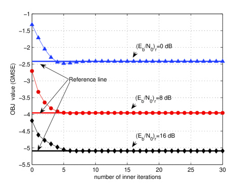
Figure 2: Objective function value (GMSE criterion) versus number of inner iterations.

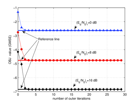
Figure 3: Objective function value (GMSE criterion) versus number of outer iterations.

In Fig. 4, we show the values of the objective function, ${\rm OBJ}$, for FD-DFE, cf. (62), for different values of $N_{fb}$. Note that ${\rm OBJ}$ for $N_{fb}=0$ serves as the upper bound, ${\rm OBJ}_{ub}$, for the general objective function. From the figure, we observe that the upper bound is very close to the objective function for all considered values of $N_{fb}$, especially for medium to high SNR and for the $\{2,3,3,3\}$ system. Therefore, ${\rm OBJ}_{ub}$ constitutes a good approximation for the objective function for the FD-DFE receiver.

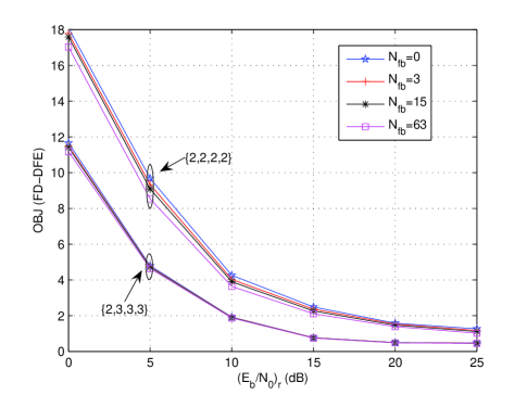
Figure 4: Objective function value of the FD-DFE receiver for different values of $N_{fb}$.

V-B Comparison of SC-FDE and OFDM for JSR Precoding

In Fig. 5, we show the BER of uncoded quaternary phase-shift keying (QPSK) as a function of $(E_{b}/N_{0})_{r}$ for the proposed FD-LE based MIMO relay system for the three considered precoding matrix optimization criteria. For FD-DFE, only the GMSE criterion is considered as for FD-DFE all three criteria are equivalent. For comparison, the performance of a MIMO-OFDM relay system optimized under the same criteria is also included [6]. The figure shows that for the $\{2,2,2,2\}$ system, the proposed MIMO relay system with an FD-LE receiver outperforms the corresponding OFDM-based system by a large margin since, in contrast to uncoded OFDM, FD-LE is able to exploit the frequency diversity offered by the channel. In addition, for both FD-LE and OFDM, the system employing the maxMSE criterion offers the best performance since the worst-case MSE is minimized. For FD-DFE, the performance improvement compared to FD-LE and OFDM is remarkable and a much higher diversity gain is observed. On the other hand, for the $\{2,3,3,3\}$ system, we observe that the performance gaps between FD-DFE, FD-LE, and OFDM become smaller. Surprisingly, using the maxMSE criterion, the optimized OFDM and FD-LE systems achieve a performance very close to that of FD-DFE. This is due to fact that the additional antennas offer additional spatial diversity which helps OFDM and FD-LE to effectively avoid the deep spectrum nulls that otherwise negatively affect their performance in frequency-selective fading.

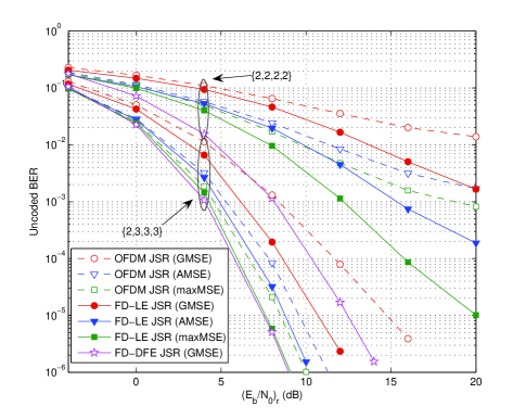
Figure 5: Uncoded BER of $\{2,2,2,2\}$ and $\{2,3,3,3\}$ MIMO relay systems for JSR precoding using different optimization criteria.

In Fig. 6, we investigate the capacity of the OFDM and SC-FDE systems with different optimization criteria. As expected, the systems optimized under the GMSE criterion have the best performance since minimizing the GMSE is equivalent to maximizing the capacity. In general, the capacity achieved by the considered MIMO-OFDM relay systems is higher than that of the corresponding FD-LE relay systems, except for the case when both systems are optimized based on the maxMSE criterion. Indeed, the OFDM system optimized under the maxMSE criterion suffers from the worst capacity performance among all the considered schemes since the available power is mainly used to improve the MSE of the subcarriers with bad channel conditions instead of taking advantage of the subcarriers with good channel conditions. In addition, Fig. 6 shows that for FD-LE, the AMSE and maxMSE criteria lead to exactly the same capacity, which implies that the unitary rotation of the source precoding matrix does not influence the capacity of the system. Furthermore, the capacity achieved with FD-DFE is larger than that achieved with any of the FD-LE schemes and very close to that of OFDM. This is due to the lower stream MSEs of FD-DFE compared to FD-LE, which translates into larger stream SINRs and larger system capacity. For the $\{2,3,3,3\}$ system, we observe that FD-LE and OFDM achieve almost the same performance for the AMSE and GMSE criteria, implying that with more source/relay/destination antennas, FD-LE will approach the achievable capacity of the OFDM system.

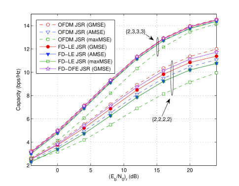
Figure 6: Capacity of $\{2,2,2,2\}$ and $\{2,3,3,3\}$ MIMO relay systems with JSR relay precoding for different optimization criteria.

V-C Performance of Suboptimal Power Allocation Schemes

In Figs. 7 and 8, we plot the uncoded and coded BERs for the suboptimal power allocation schemes discussed in Section IV-D for a {2,2,2,2} system, respectively. For the coded case, the standard rate-1/2 convolution code with generator matrix $(133,171)_{oct}$ is adopted. The OFDM and FD-LE systems are both optimized under the maxMSE criterion. The FD-DFE system is optimized under the GMSE criterion since for FD-DFE all three considered criteria are equivalent to the GMSE criterion. From Fig. 7 we observe that for uncoded transmission, the FD-LE system outperforms the OFDM system if both employ the same precoding technique. Fig. 7 also shows that for FD-LE and OFDM, EPA-S and ROP suffer from a considerable performance degradation compared to JSR, while for FD-DFE, the performance loss is relatively small for UPS and almost negligible for EPA-S. By coding across subcarriers, OFDM-based relay systems can also exploit the frequency diversity of the channel and significantly improve their BER performance, cf. Fig. 8. Nevertheless, the coded FD-LE system still outperforms the OFDM system if the same precoding technique is assumed in both cases. Also, Fig. 8 reveals that channel coding significanlty reduces the performance loss caused by suboptimal precoding techniques for both OFDM and FD-LE.

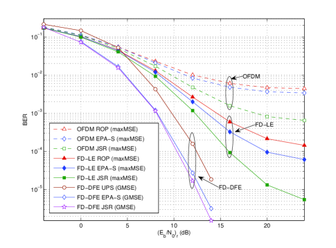
Figure 7: Uncoded BER of a $\{2,2,2,2\}$ MIMO relay system with JSR and suboptimal precoding schemes.

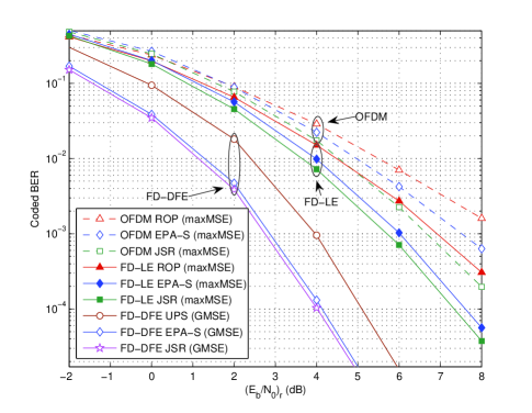
Figure 8: Coded BER of a $\{2,2,2,2\}$ MIMO relay system with JSR and suboptimal precoding schemes.

Since the performance of FD-DFE depends on the the number of FBF taps, in Fig. 9, we investigate the influence of $N_{fb}$ on the performance of a {2,2,2,2} system. The results show that while the value of $N_{fb}$ has limited impact on the performance of EPA-S, it does play a critical role for UPS. The reason is that for EPA-S, the equivalent $S$-$R$-$D$ channel is diagonalized into $M$ parallel channels, thus eliminating the inter-stream interference at the receiver. However, for the case of UPS , the equivalent end-to-end channel is not fully diagonalized and the received symbols experience inter-stream interference. Consequently, a FBF with sufficiently large $N_{fb}$ is required to cancel out this interference. As can be inferred from Fig. 9, there is a complexity tradeoff between the transmitter and the receiver for FD-DFE. For EPA-S, since a small number of FBF taps (e.g., $N_{fb}=3$) is sufficient to achieve good performance, the receiver complexity is similar to that of FD-LE. However, comparatively complex FD signal processing has to be carried out at the transmitter. This characteristic makes EPA-S suitable for the downlink transmission. For the UPS scheme, on the other hand, the transmit processing is very simple since the single tap precoding matrix ${\mathbf{V}}_{1}$ can be directly implemented in the TD. In addition, the feedback overhead is low as ${\mathbf{V}}_{1}$ is identical for all frequency tones. However, UPS requires a longer and thus more complex FBF to achieve a high performance. These characteristics make UPS a very promising scheme for uplink transmission.

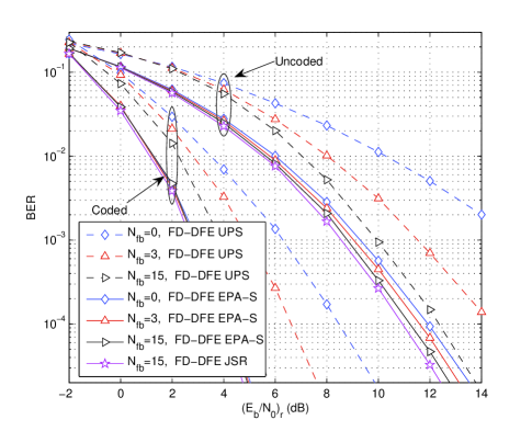
Figure 9: Uncoded and coded BER of a $\{2,2,2,2\}$ MIMO relay system with FD-DFE using JSR and suboptimal precoding schemes with different numbers of FBF taps.

VI Conclusion

In this paper, we have tackled the problem of transceiver design for MIMO relay systems employing SC-FDE. The optimal MMSE FD-LE and FD-DFE filters at the destination were derived, and the optimal structures of the source and relay precoding matrices were obtained in closed form for a general family of objective functions. For systems employing an FD-DFE receiver, we first showed that the considered objective functions are all equivalent and derived an upper bound on the original objective functions, which was shown to be equal to the GMSE objective function for the FD-LE receiver. The remaining power allocation problem was solved globally by using a high SNR approximation of the objective function and efficient convex optimization methods. Our results show that the proposed SC-FDE relaying schemes outperform the corresponding OFDM schemes in terms of both coded and uncoded BER. In addition, the performance gap between SC-FDE and OFDM relay systems decreases when the number of source/relay/destination antennas is larger than the number of data streams. Furthermore, we have shown that the proposed suboptimal power allocation schemes can reduce the system complexity and feedback overhead at the expense of a moderate performance degradation, especially in case of coded transmission, making them promising candidates for practical relay systems.

Appendix

We first provide some relevant definitions and lemmas that will be used in the proof.

Definition 1 [15,1.A.1]: Given two $N\times 1$ real vectors ${\mathbf{x}},{\mathbf{y}}\in\mathbb{R}^{N}$. Let $x_{[1]},\cdots,x_{[N]}$ and $y_{[1]},\cdots,y_{[N]}$ denote the components of ${\mathbf{x}}$ and ${\mathbf{y}}$ in decreasing order. Then, ${\mathbf{x}}$ is majorized by ${\mathbf{y}}$, or ${\mathbf{x}}\prec{\mathbf{y}}$, if $\sum_{i=1}^{k}x_{[i]}\leq\sum_{i=1}^{k}y_{[i]}$ for $k<N$ and $\sum_{i=1}^{N}x_{[i]}=\sum_{i=1}^{N}y_{[i]}$. Vector ${\mathbf{x}}$ is weakly majorized by ${\mathbf{y}}$, or ${\mathbf{x}}\prec_{w}{\mathbf{y}}$, if $\sum_{i=1}^{k}x_{[i]}\leq\sum_{i=1}^{k}y_{[i]},\forall k$.

Definition 2 [15,3.A.1]: A real function $f$ is Schur-convex if for ${\mathbf{x}}\prec{\mathbf{y}}$, we have $f({\mathbf{x}})\leq f({\mathbf{y}})$. Similarly, $f$ is Schur-concave if for ${\mathbf{x}}\prec{\mathbf{y}}$, we have $f({\mathbf{x}})\geq f({\mathbf{y}})$.

Lemma 1 [15,9.B.1]: For a Hermitian matrix ${\mathbf{A}}$ with $\mbox{diag}[{\mathbf{A}}]$ and $\lambda({\mathbf{A}})$ denoting vectors containing the main diagonal elements and the eigenvalues of ${\mathbf{A}}$ arranged in decreasing order, respectively, we have $\mbox{diag}[{\mathbf{A}}]\prec\lambda({\mathbf{A}})$.

Lemma 2 [15,9.H.2]: For $M$ matrices ${\mathbf{A}}_{i}\in\mathbb{C}^{N\times N},i=1,\cdots,M$, let ${\mathbf{B}}={\mathbf{A}}_{1}{\mathbf{A}}_{2}\cdots{\mathbf{A}}_{M}$. Then, $\mathbf{\sigma}({\mathbf{B}})\prec_{w}\mathbf{\sigma}({\mathbf{A}}_{1})\odot\mathbf{\sigma}({\mathbf{A}}_{2})\odot\cdots\mathbf{\sigma}({\mathbf{A}}_{M})$, where $\mathbf{\sigma}({\mathbf{X}})$ denotes the vector containing the singular values of matrix ${\mathbf{X}}$ arranged in decreasing order and $\odot$ denotes the element-wise product of two vectors.

Lemma 3 [15,3.A.8]: A real function $f$ satisfies ${\mathbf{x}}\prec_{w}{\mathbf{y}}\Rightarrow f({\mathbf{x}})\leq f({\mathbf{y}})$ if and only if $f$ is Schur-convex and increasing.

Lemma 4 [15,9.H.1]: For two Hermitian positive semidefinite matrices $\{{\mathbf{A}},{\mathbf{B}}\}\in\mathbb{C}^{N\times N}$ with eigenvalues $\lambda_{{\mathbf{A}},i},\lambda_{{\mathbf{B}},i}$, arranged in the same order, we have ${\rm tr}({\mathbf{A}}{\mathbf{B}})\geq\sum_{i=1}^{N}\lambda_{{\mathbf{A}},i}\lambda_{{\mathbf{B}},N-i+1}$.

Lemma 5 [15, p.7]: For a vector ${\mathbf{x}}\in\mathbb{C}^{N\times 1}$, we have $\sum_{i=1}^{N}(x_{i}/N)\mathbf{1}\prec{\mathbf{x}}$, where $\mathbf{1}$ is the all-ones vector.

Lemma 6: For Hermitian matrices ${\mathbf{A}}_{k}$ and $\hat{\mathbf{A}}_{k}$, $k=1,2,\cdots,N_{c}$ , if $\mbox{diag}[{\mathbf{A}}_{k}]\prec\mbox{diag}[\hat{\mathbf{A}}_{k}]$, we have $\mbox{diag}[\sum_{k=1}^{N_{c}}{\mathbf{A}}_{k}]\prec\mbox{diag}[\sum_{k=1}^{N_{c}}\hat{\mathbf{A}}_{k}]$.

Proof: According to Definition 1, if $\mbox{diag}[{\mathbf{A}}_{k}]\prec\mbox{diag}[\hat{\mathbf{A}}_{k}]$, we have $\sum_{i=1}^{j}a_{[ki]}\leq\sum_{i=1}^{j}\hat{a}_{[ki]}$ for $j<N$ and $\sum_{i=1}^{N}a_{[ki]}=\sum_{i=1}^{N}\hat{a}_{[ki]}$ for $j=N$, where $a_{[ki]}$ and $\hat{a}_{[ki]}$ are the $i$th diagonal entries of ${\mathbf{A}}_{k}$ and $\hat{\mathbf{A}}_{k}$, respectively. Since $a_{[ki]}$ and $\hat{a}_{[ki]},\forall k,i$, are non-negative, we have $\sum_{k=1}^{N_{c}}\sum_{i=1}^{j}a_{[ki]}\leq\sum_{k=1}^{N_{c}}\sum_{i=1}^{j}\hat{a}_{[ki]}$ for $j<N$ and $\sum_{k=1}^{N_{c}}\sum_{i=1}^{N}a_{[ki]}=\sum_{k=1}^{N_{c}}\sum_{i=1}^{N}\hat{a}_{[ki]}$ for $j=N$. Therefore, we have $\sum_{k=1}^{N_{c}}\mbox{diag}[{\mathbf{A}}_{k}]$$\prec\sum_{k=1}^{N_{c}}\mbox{diag}[\hat{\mathbf{A}}_{k}]$, which is equivalent to $\mbox{diag}[\sum_{k=1}^{N_{c}}{\mathbf{A}}_{k}]\prec\mbox{diag}[\sum_{k=1}^{N_{c}}\hat{\mathbf{A}}_{k}]$.

Lemma 7 [15, 9.B.2]: For a diagonal matrix ${\mathbf{D}}\in\mathbb{C}^{M\times M}$, there is a unitary matrix ${\mathbf{U}}$ such that ${\mathbf{A}}={\mathbf{U}}^{\dagger}{\mathbf{D}}{\mathbf{U}}$ has identical diagonal entries equal to ${\rm tr}({\mathbf{D}})/M$.

We now set out to prove the optimal structure of the source and relay precoding matrices when $f(\mbox{diag}[\hat{\mathbf{E}}])$ is a Schur-concave increasing function w.r.t. $\mbox{diag}[\hat{\mathbf{E}}]$. Let us begin with the core term in the expression for $\hat{\mathbf{E}}$ in (12), which is given by

$$\mathbf{\Psi}_{k}^{-1}= {\mathbf{I}}_{M}-$$

$$\underbrace{\sigma_{s}^{2}{\mathbf{Q}}_{k}^{\dagger}(\sigma_{s}^{2}{\mathbf{Q}}_{k}{\mathbf{Q}}_{k}^{\dagger}+\sigma_{v}^{2}{\mathbf{H}}_{k}{\mathbf{A}}_{k}{\mathbf{A}}_{k}^{\dagger}{\mathbf{H}}_{k}^{\dagger}+\sigma_{u}^{2}{\mathbf{I}}_{N_{d}})^{-1}{\mathbf{Q}}_{k}}_{\mathbf{\Upsilon}_{k}},$$ (71)

where we employed the matrix inversion lemma. The CV matrix can now be expressed as

$$\hat{\mathbf{E}}=\frac{\sigma_{s}^{2}}{N_{c}}\sum_{k=1}^{N_{c}}\mathbf{\Psi}_{k}^{-1}=\frac{\sigma_{s}^{2}}{N_{c}}(N_{c}{\mathbf{I}}_{M}-\sum_{k=1}^{N_{c}}\mathbf{\Upsilon}_{k}).$$ (72)

Since $f(\mbox{diag}[\sigma_{s}^{2}{\mathbf{I}}_{M}-\frac{\sigma_{s}^{2}}{N_{c}}\sum_{k=1}^{N_{c}}\mathbf{\Upsilon}_{k}])$ is a Schur-concave decreasing function w.r.t. $\mbox{diag}[\sum_{k=1}^{N_{c}}\mathbf{\Upsilon}_{k}]$, $-f(\mbox{diag}[\sigma_{s}^{2}{\mathbf{I}}_{M}-\frac{\sigma_{s}^{2}}{N_{c}}\sum_{k=1}^{N_{c}}\mathbf{\Upsilon}_{k}])$ is a Schur-convex increasing function w.r.t. $\mbox{diag}[\sum_{k=1}^{N_{c}}\mathbf{\Upsilon}_{k}]$. $\mathbf{\Upsilon}_{k}$ can be further expressed as

$$\mathbf{\Upsilon}_{k} = {\mathbf{X}}_{k}^{\dagger}{\mathbf{Y}}_{k}^{\dagger}({\mathbf{J}}_{k}{\mathbf{J}}_{k}^{{\dagger}}+\sigma_{u}^{2}{\mathbf{I}}_{N_{d}})^{-1}{\mathbf{Y}}_{k}{\mathbf{X}}_{k},$$ (73)

where we have used the definitions

$${\mathbf{X}}_{k} = \sigma_{s}{\mathbf{G}}_{k}{\mathbf{P}}_{k},\quad{\mathbf{Y}}_{k}={\mathbf{H}}_{k}{\mathbf{A}}_{k},$$

$${\mathbf{J}}_{k} = {\mathbf{Y}}_{k}({\mathbf{X}}_{k}{\mathbf{X}}_{k}^{{\dagger}}+\sigma_{v}^{2}{\mathbf{I}}_{N_{r}})^{1/2}.$$ (74)

By rewriting ${\mathbf{Y}}_{k}$ in terms of ${\mathbf{X}}_{k}$ and ${\mathbf{J}}_{k}$, we obtain ${\mathbf{Y}}_{k}={\mathbf{J}}_{k}({\mathbf{X}}_{k}{\mathbf{X}}_{k}^{{\dagger}}+\sigma_{v}^{2}{\mathbf{I}}_{N_{r}})^{-1/2}$. Plugging this result into (73) leads to

$$\mathbf{\Upsilon}_{k}= {\mathbf{X}}_{k}({\mathbf{X}}_{k}{\mathbf{X}}_{k}^{{\dagger}}+\sigma_{v}^{2}{\mathbf{I}}_{N_{r}})^{-1/2}{\mathbf{J}}_{k}^{\dagger}({\mathbf{J}}_{k}{\mathbf{J}}_{k}^{{\dagger}}+\sigma_{u}^{2}{\mathbf{I}}_{N_{d}})^{-1}$$

$${\mathbf{J}}_{k}({\mathbf{X}}_{k}{\mathbf{X}}_{k}^{{\dagger}}+\sigma_{v}^{2}{\mathbf{I}}_{N_{r}})^{-1/2}{\mathbf{X}}_{k}.$$ (75)

Now, we define the following SVDs

$${\mathbf{X}}_{k}={\mathbf{U}}_{X}^{(k)}\mathbf{\Lambda}_{X}^{(k)}{\mathbf{V}}_{X}^{(k)},\quad{\mathbf{J}}_{k}={\mathbf{U}}_{J}^{(k)}\mathbf{\Lambda}_{J}^{(k)}{\mathbf{V}}_{J}^{(k)},$$

$$({\mathbf{X}}_{k}{\mathbf{X}}_{k}^{{\dagger}}+\sigma_{v}^{2}{\mathbf{I}}_{N_{r}})^{-1/2}={\mathbf{U}}_{X}^{(k)}(\mathbf{\Lambda}_{X}^{(k)2}+\sigma_{v}^{2}{\mathbf{I}}_{M})^{-1/2}\mathbf{\Omega}^{(k)},$$ (76)

where ${\mathbf{U}}_{X}^{(k)}\in\mathbb{C}^{N_{r}\times M}$, ${\mathbf{U}}_{J}^{(k)}\in\mathbb{C}^{N_{d}\times M}$, $\{{\mathbf{V}}_{J}^{(k)},\mathbf{\Omega}^{(k)}\}\in\mathbb{C}^{M\times N_{r}}$, $\{\mathbf{\Lambda}_{X}^{(k)},{\mathbf{V}}_{X}^{(k)},\mathbf{\Lambda}_{J}^{(k)}\}\in\mathbb{C}^{M\times M}$.The diagonal entries of $\mathbf{\Lambda}_{X}^{(k)}$ and $\mathbf{\Lambda}_{J}^{(k)}$ are both sorted in increasing order. We can use (76) to rewrite (Appendix) as

$$\mathbf{\Upsilon}_{k}= {\mathbf{V}}_{X}^{(k){\dagger}}\mathbf{\Lambda}_{X}^{(k)}{{\mathbf{Q}}_{2}^{(k){\dagger}}}(\mathbf{\Lambda}_{X}^{(k)2}+\sigma_{v}^{2}{\mathbf{I}}_{M})^{-1/2}{{{\mathbf{Q}}_{1}^{(k){\dagger}}}}$$

$$\times({\mathbf{I}}_{M}+\sigma_{u}^{2}\mathbf{\Lambda}_{J}^{(k)-2})^{-1}{{{\mathbf{Q}}_{1}^{(k)}}}(\mathbf{\Lambda}_{X}^{(k)2}+\sigma_{v}^{2}{\mathbf{I}}_{M})^{-1/2}$$

$$\times{{{\mathbf{Q}}_{2}^{(k)}}}\mathbf{\Lambda}_{X}^{(k)}{\mathbf{V}}_{X}^{(k)},$$ (77)

where ${\mathbf{Q}}_{1}^{(k)}=\mathbf{{\mathbf{V}}}_{J}^{(k)}{\mathbf{U}}_{X}^{(k)}$ and ${\mathbf{Q}}_{2}^{(k)}=\mathbf{\Omega}^{(k)}{\mathbf{U}}_{X}^{(k)}$. By applying Lemmas 1 and 2, we obtain

$$\mbox{diag}[\mathbf{\Upsilon}_{k}] \prec\mathbf{\lambda}(\mathbf{\Upsilon}_{k})$$

$$\prec_{w}\mbox{diag}[\underbrace{({\mathbf{I}}_{M}+\sigma_{v}^{2}\mathbf{\Lambda}_{X}^{(k)-2})^{-1}}_{{\mathbf{D}}_{1}^{(k)}}\underbrace{({\mathbf{I}}_{M}+\sigma_{u}^{2}\mathbf{\Lambda}_{J}^{(k)-2})^{-1}}_{{\mathbf{D}}_{2}^{(k)}}].$$ (78)

Therefore, $\mbox{diag}[\mathbf{\Upsilon}_{k}]$ is majorized by $\mbox{diag}[{\mathbf{D}}_{1}^{(k)}{\mathbf{D}}_{2}^{(k)}]$ when ${\mathbf{V}}_{X}^{(k)}=\mathbf{\Xi}_{1}$, ${\mathbf{Q}}_{2}^{(k)}=\mathbf{\Xi}_{2}$, ${\mathbf{Q}}_{1}^{(k)}=\mathbf{\Xi}_{3}$, where $\mathbf{\Xi}_{i}\in\mathbb{C}^{M\times M},\forall i$, are arbitrary diagonal matrices with unit norm diagonal elements. Without loss of generality, we can choose $\mathbf{\Xi}_{i}={\mathbf{I}}_{M},\forall i$. Hence, we have

$${\mathbf{V}}_{X}^{(k)} = {\mathbf{I}}_{M},\quad\mathbf{\Omega}^{(k)}={\mathbf{U}}_{X}^{(k){\dagger}},\quad\mathbf{{\mathbf{V}}}_{J}^{(k)}={\mathbf{U}}_{X}^{(k){\dagger}}.$$ (79)

According to Lemma 6,

$$\mbox{diag}[\sum_{k=1}^{N_{c}}\mathbf{\Upsilon}_{k}]\prec_{w}\mbox{diag}[\sum_{k=1}^{N_{c}}({\mathbf{D}}_{1}^{(k)}{\mathbf{D}}_{2}^{(k)})]$$ (80)

holds. From the fact that $-f(\mbox{diag}[\sigma_{s}^{2}{\mathbf{I}}_{M}-\frac{\sigma_{s}^{2}}{N_{c}}\sum_{k=1}^{N_{c}}\mathbf{\Upsilon}_{k}])$ is a Schur-convex increasing function w.r.t. $\mbox{diag}[\sum_{k=1}^{N_{c}}\mathbf{\Upsilon}_{k}]$, (80), and Definition 2, we deduce that $-f(\mbox{diag}[\sigma_{s}^{2}{\mathbf{I}}_{M}-\frac{\sigma_{s}^{2}}{N_{c}}\sum_{k=1}^{N_{c}}\mathbf{\Upsilon}_{k}])\leq-f(\mbox{diag}[\sigma_{s}^{2}{\mathbf{I}}_{M}-\frac{\sigma_{s}^{2}}{N_{c}}\sum_{k=1}^{N_{c}}{\mathbf{D}}_{1}^{(k)}{\mathbf{D}}_{2}^{(k)}])$, which is equivalent to

$$f(\mbox{diag}[\sigma_{s}^{2}{\mathbf{I}}_{M}-\frac{\sigma_{s}^{2}}{N_{c}}\sum_{k=1}^{N_{c}}\mathbf{\Upsilon}_{k}])$$

$$\geq f(\mbox{diag}[\sigma_{s}^{2}{\mathbf{I}}_{M}-\frac{\sigma_{s}^{2}}{N_{c}}\sum_{k=1}^{N_{c}}{\mathbf{D}}_{1}^{(k)}{\mathbf{D}}_{2}^{(k)}]).$$ (81)

Therefore, with the help of the matrices in (79), the value of the objective function can be reduced to $f(\mbox{diag}[\sigma_{s}^{2}{\mathbf{I}}_{M}-\frac{\sigma_{s}^{2}}{N_{c}}\sum_{k=1}^{N_{c}}{\mathbf{D}}_{1}^{(k)}{\mathbf{D}}_{2}^{(k)}])$.

In the following, we derive the structure of the optimal source and relay precoding matrices minimizing the power consumption of the source and the relay. For simplicity of notation, we only consider the case when $N_{s}=N_{r}=N_{d}$. The proof can be easily extended to the case where $N_{s}$, $N_{r}$, and $N_{d}$ have different values. From (76), we have $\sigma_{s}{\mathbf{U}}_{G}^{(k)}\mathbf{\Lambda}_{G}^{(k)}{\mathbf{V}}_{G}^{(k){\dagger}}{\mathbf{P}}_{k}={\mathbf{U}}_{X}^{(k)}\mathbf{\Lambda}_{X}^{(k)}{\mathbf{V}}_{X}^{(k)}$, which can be used to express the source power consumption at frequency tone $k$ as

$$\sigma_{s}^{2}{\rm tr}({\mathbf{P}}_{k}{\mathbf{P}}_{k}^{\dagger})$$

$$={\rm tr}(\mathbf{\Lambda}_{G}^{(k)-1}\underbrace{{\mathbf{U}}_{G}^{(k){\dagger}}{\mathbf{U}}_{X}^{(k)}}_{{\mathbf{Q}}_{3}^{(k){\dagger}}}\mathbf{\Lambda}_{X}^{(k)2}\underbrace{{\mathbf{U}}_{X}^{(k){\dagger}}{\mathbf{U}}_{G}^{(k)}}_{{\mathbf{Q}}_{3}^{(k)}}\mathbf{\Lambda}_{G}^{(k)-1})$$

$$\geq{\rm tr}(\mathbf{\bar{\Lambda}}_{G}^{(k)-2}\mathbf{\Lambda}_{X}^{(k)2}),$$ (82)

where the inequality follows from Lemma 4, and the diagonal matrix $\mathbf{\bar{\Lambda}}_{G}^{(k)}\in\mathbb{C}^{M\times M}$ contains the $M$ largest singular values of ${{\mathbf{G}}}_{k}$. Therefore, in order to minimize the source power, we need to choose ${\mathbf{Q}}_{3}^{(k)}=[{\mathbf{I}}_{M}\;\;\mathbf{0}_{M\times(N_{s}-M)}]^{T}$, i.e., ${\mathbf{U}}_{X}^{(k)}={\bar{\mathbf{U}}}_{G}^{(k)}$, where ${\bar{\mathbf{U}}}_{G}^{(k)}$ contains the $M$ right-most columns of ${\mathbf{U}}_{G}^{(k)}$. Recalling from (82) that ${\mathbf{V}}_{X}^{(k)}={\mathbf{I}}_{M}$, the source matrix can be expressed as

$${\mathbf{P}}_{k}=\frac{1}{\sigma_{s}}\bar{\mathbf{V}}_{G}^{(k)}\mathbf{\bar{\Lambda}}_{G}^{(k)-1}\mathbf{\Lambda}_{X}^{(k)}=\bar{\mathbf{V}}_{G}^{(k)}\mathbf{\Lambda}_{P}^{(k)},$$ (83)

where $\bar{\mathbf{V}}_{G}^{(k)}$ contains the $M$ right-most columns of ${\mathbf{V}}_{G}^{(k)}$ and $\mathbf{\Lambda}_{P}^{(k)}\triangleq\frac{1}{\sigma_{s}}\mathbf{\bar{\Lambda}}_{G}^{(k)-1}\mathbf{\Lambda}_{X}^{(k)}$. Next, from (76) we obtain ${\mathbf{U}}_{H}^{(k)}\mathbf{\Lambda}_{H}^{(k)}{\mathbf{V}}_{H}^{(k){\dagger}}{\mathbf{A}}_{k}={\mathbf{J}}_{k}({\mathbf{X}}_{k}{\mathbf{X}}_{k}^{\dagger}+\sigma_{v}^{2}{\mathbf{I}}_{N_{d}})^{-1/2}$. Using this result, we can express the relay power consumption at frequency tone $k$ as

$${\rm tr}({\mathbf{A}}_{k}({\mathbf{X}}_{k}{\mathbf{X}}_{k}^{\dagger}+\sigma_{v}^{2}{\mathbf{I}}_{N_{r}}){\mathbf{A}}_{k}^{\dagger})$$

$$={\rm tr}(\mathbf{\Lambda}_{H}^{(k)-1}{\mathbf{U}}_{H}^{(k){\dagger}}{\mathbf{J}}_{k}{\mathbf{J}}_{k}^{\dagger}{\mathbf{U}}_{H}^{(k)}\mathbf{\Lambda}_{H}^{(k)-1})$$

$$={\rm tr}(\mathbf{\Lambda}_{H}^{(k)-1}\underbrace{{\mathbf{U}}_{H}^{(k){\dagger}}{\mathbf{U}}_{J}^{(k)}}_{{\mathbf{Q}}_{4}^{(k){\dagger}}}\mathbf{\Lambda}_{J}^{(k)2}\underbrace{{\mathbf{U}}_{J}^{(k){\dagger}}{\mathbf{U}}_{H}^{(k)}}_{{\mathbf{Q}}_{4}^{(k)}}\mathbf{\Lambda}_{H}^{(k)-1})$$

$$\geq{\rm tr}(\bar{\mathbf{\Lambda}}_{H}^{(k)-2}\mathbf{\Lambda}_{J}^{(k)2}),$$ (84)

where the inequality follows from Lemma 4, and the diagonal matrix $\mathbf{\bar{\Lambda}}_{H}^{(k)}\in\mathbb{C}^{M\times M}$ contains the $M$ largest singular values of ${{\mathbf{H}}_{k}}$. In (84), equality holds for ${\mathbf{Q}}_{4}^{(k)}=[{\mathbf{I}}_{M}$   $\mathbf{0}_{M\times(N_{r}-M)}]^{T}$, i.e., ${\mathbf{U}}_{J}^{(k)}=\bar{\mathbf{U}}_{H}^{(k)}$, where $\bar{\mathbf{U}}_{H}^{(k)}$ contains the $M$ right-most columns of ${\mathbf{U}}_{H}^{(k)}$. Recalling from (79) that ${{\mathbf{U}}_{X}^{(k)}}^{\dagger}=\mathbf{\Omega}^{(k)}={\mathbf{V}}_{J}^{(k)}$, and from (82) that ${\mathbf{U}}_{X}^{(k)}=\bar{\mathbf{U}}_{G}^{(k)}$, we obtain for ${\mathbf{A}}_{k}$ the expression

$${\mathbf{A}}_{k} = \bar{\mathbf{V}}_{H}^{(k)}\mathbf{\bar{\Lambda}}_{H}^{(k)-1}\mathbf{\Lambda}_{J}^{(k)}(\mathbf{\Lambda}_{X}^{(k)2}+\sigma_{v}^{2}{\mathbf{I}}_{M})^{-1/2}\bar{\mathbf{U}}_{G}^{(k){\dagger}}$$ (85)

$$= \bar{\mathbf{V}}_{H}^{(k)}\mathbf{\Lambda}_{A}^{(k)}\bar{\mathbf{U}}_{G}^{(k){\dagger}},$$

where $\bar{\mathbf{V}}_{H}^{(k)}$ and $\bar{\mathbf{U}}_{G}^{(k)}$ contain the $M$ right-most columns of ${\mathbf{V}}_{H}^{(k)}$ and ${\mathbf{U}}_{G}^{(k)}$, respectively, and $\mathbf{\Lambda}_{A}^{(k)}\triangleq\mathbf{\bar{\Lambda}}_{H}^{(k)-1}\mathbf{\Lambda}_{J}^{(k)}(\mathbf{\Lambda}_{X}^{(k)2}+\sigma_{v}^{2}{\mathbf{I}}_{M})^{-1/2}$. Hence, we have proved that the expressions for the source and relay precoding matrices given in (83) and (85) minimize the objective function $f(\mbox{diag}[\hat{\mathbf{E}}])$, cf. (81), as well as the power consumption at the source and the relay, cf. (82) and (84).

Now, we turn our attention to the case when $f(\mbox{diag}[\hat{\mathbf{E}}])$ is a Schur-convex increasing function w.r.t. $\mbox{diag}[\hat{\mathbf{E}}]$. From Lemma 5 we know that $\frac{1}{M}{\rm tr}(\hat{\mathbf{E}})\mathbf{1}\prec\mbox{diag}[\hat{\mathbf{E}}]$. Combining this fact and Definition 2, we obtain the inequality

$$f(\mbox{diag}[\hat{\mathbf{E}}])\geq f(\frac{1}{M}{\rm tr}(\hat{\mathbf{E}})\mathbf{1}),$$ (86)

where equality holds when the diagonal entries of $\hat{\mathbf{E}}$ are all equal to $\frac{1}{M}{\rm tr}(\hat{\mathbf{E}})$. In the following, we show that by applying a unitary rotation to the source precoding matrix, we can achieve this equality. Using the eigenvalue decomposition ${\mathbf{Q}}_{k}^{\dagger}{\mathbf{K}}_{k}^{-1}{\mathbf{Q}}_{k}={\mathbf{U}}_{E}^{(k)}\mathbf{\Lambda}_{E}^{(k)}{\mathbf{U}}_{E}^{(k){\dagger}}$, we can write $\mathbf{\Psi}_{k}^{-1}={\mathbf{U}}_{E}^{(k)}({\mathbf{I}}_{M}+\mathbf{\Lambda}_{E}^{(k)})^{-1}{\mathbf{U}}_{E}^{(k){\dagger}}$. Let us consider the feasible source precoding matrix $\bar{\mathbf{P}}_{k}={\mathbf{P}}_{k}{\mathbf{U}}_{E}^{(k)}{\mathbf{V}}_{0}$, where ${\mathbf{V}}_{0}$ is a unitary matrix and thus does not affect the power constraints. Replacing ${\mathbf{P}}_{k}$ with $\bar{\mathbf{P}}_{k}$ in $\mathbf{\Psi}_{k}^{-1}$, we arrive at

$$\mathbf{\Psi}_{k}^{-1}={\mathbf{V}}_{0}^{\dagger}({\mathbf{I}}_{M}+\mathbf{\Lambda}_{E}^{(k)})^{-1}{\mathbf{V}}_{0},$$ (87)

which allows us to express the error CV matrix as

$$\hat{\mathbf{E}}=\frac{\sigma_{s}^{2}}{N_{c}}\mathbf{\sum}_{k=1}^{N_{c}}\mathbf{\Psi}_{k}^{-1}=\frac{\sigma_{s}^{2}}{N_{c}}{\mathbf{V}}_{0}^{\dagger}\sum_{k=1}^{N_{c}}({\mathbf{I}}_{M}+\mathbf{\Lambda}_{E}^{(k)})^{-1}{\mathbf{V}}_{0}.$$ (88)

Since $\sum_{k=1}^{N_{c}}({\mathbf{I}}_{M}+\mathbf{\Lambda}_{E}^{(k)})^{-1}$ is the sum of $N_{c}$ diagonal matrices, it is also a diagonal matrix. Based on Lemma 7, we conclude that there exists a unitary matrix ${\mathbf{V}}_{0}$ such that $\hat{\mathbf{E}}$ has identical diagonal elements given by $\frac{1}{M}{\rm tr}(\hat{\mathbf{E}})$. Since the objective function is an increasing function w.r.t. its arguments, minimizing the original Schur-convex objective function is now equivalent to minimizing $\frac{1}{M}{\rm tr}(\hat{\mathbf{E}})$, which is a Schur-concave function. Therefore, the optimal structures of ${\mathbf{P}}_{k}$ and ${\mathbf{A}}_{k}$ are given by (83) and (85), respectively. Furthermore, as the resulting ${\mathbf{U}}_{E}^{(k)}$ can be shown to be an identity matrix, the source precoding matrix for Schur-convex functions is given by $\bar{\mathbf{P}}_{k}={\mathbf{P}}_{k}{\mathbf{V}}_{0}=\bar{\mathbf{V}}_{G}^{(k)}\mathbf{\Lambda}_{P}^{(k)}{\mathbf{V}}_{0}$.

References

- [1] R. Nabar, H. Bölcskei, and F. Kneubühler, “Fading relay channels: Performance limits and space-time signal design,” IEEE J. Sel. Areas Commun, vol. 22, pp. 1099–1109, 2004.
- [2] I. Hammerstrom and A. Wittneben, “Power allocation schemes for amplify-and-forward MIMO-OFDM relay links,” IEEE Trans. Wireless. Commun., vol. 6, pp. 2798–2802, 2007.
- [3] R. Mo and Y. Chew, “Precoder design for non-regenerative MIMO relay systems,” IEEE Trans. Wireless. Commun., vol. 8, pp. 5041-5049, 2007.
- [4] F. S. Tseng, W. R. Wu and J. Y. Wu, “Joint source/relay precoder design in nonregenerative cooperative systems using an MMSE criterion,” IEEE Trans. Wireless. Commun., vol. 8, pp. 4928–4933, 2009.
- [5] R. Mo and Y. Chew, “MMSE-based joint source and relay precoding design for amplify-and-forward MIMO relay networks,” IEEE Trans. Wireless. Commun., vol. 8, pp. 4668-4676, 2009.
- [6] Y. Rong, X. Tang, and Y. Hua, “A unified framework for optimizing linear nonregenerative multicarrier MIMO relay communication systems,” IEEE Trans. Signal Process., vol. 57, pp. 4837-4851, 2009.
- [7] Y. Rong and Y. Hua, “Optimality of diagonalization of multi-hop MIMO relays,” IEEE Trans. Wireless Commun., vol. 8, pp. 6068-6077, 2009.
- [8] Y. Rong, “Optimal linear non-regenerative multi-hop MIMO relays with MMSE-DFE receiver at the destination,” IEEE Trans. Wireless Commun., vol. 9, pp. 2268–2279, 2010.
- [9] C. Xing, S. Ma, Y. C. Wu, and T. S. Ng, “Transceiver design for dual-hop nonregenerative MIMO-OFDM relay systems under channel uncertainties”, IEEE Trans. Signal Process., vol. 58, pp. 6325–6339, 2010.
- [10] C. Jeong, B. Seo, S. Lee, H. Kim, and I. Kim, “Relay precoding for non-regenerative MIMO relay systems with partial CSI feedback,” IEEE Trans. Wireless Commun., vol. 11, pp. 1698–1711, 2012.
- [11] D. Falconer, S. Ariyavisitakul, A. Benyamin-Seeyar, and B. Eidson, “Frequency domain equalization for single-carrier broadband wireless systems,” IEEE Commun. Mag., vol. 40, pp. 58–66, 2002.
- [12] F. Pancaldi, G. Vitetta, R. Kalbasi, N. Al-Dhahir, M. Uysal,and H. Mheidat, “Single-carrier frequency domain equalization,” IEEE Signal Process. Mag., vol. 25, pp. 37–56, 2008.
- [13] N. Al-Dhahir, and A. H. Sayed, “The finite-length multi-input multi-output MMSE-DFE,” IEEE Trans. Signal Process., vol. 48, pp. 2921–2936, 2000.
- [14] D. P. Palomar, J. M. Cioffi, and M. A. Lagunas, “Joint Tx-Rx beamforming design for multicarrier MIMO channels: A unified framework for convex optimization,” IEEE Trans. Signal Process., vol. 51, pp. 2381-2401, 2003.
- [15] A. W. Marshall, I. Olkin, and B. Arnold, Inequalities: theory of majorization and its applications. Springer Verlag, 2010.
- [16] J. K. Zhang, A. Kavcic, and K. M. Wong, “Equal-diagonal QR decomposition and its application to precoder design for successive-cancellation detection,” IEEE Trans. Information Theory., vol. 51, pp. 154-172, 2005.
- [17] Y. Jiang, J. Li, and W. W. Hager, “Joint transceiver design for MIMO communications using geometric mean decomposition,” IEEE Trans. Signal Process., vol. 53, pp. 3791-3803, 2005.
- [18] R. A. Horn and C. R. Johnson. Matrix Analysis, Cambridge University Press, 1985.
- [19] S. Boyd and L. Vandenberghe, Convex Optimization. Cambridge, U.K.: Cambridge Univ. Press, 2004.
- [20] T. S. Rappaport, Wireless Communications: Principles and Practice. Prentice Hall, 2002.