AKARI OBSERVATIONS OF BROWN DWARFS. III. CO, CO₂ and CH₄ FUNDAMENTAL BANDS AND PHYSICAL PARAMETERS

Abstract

We investigate variations in the strengths of three molecular bands, $\mathrm{CH_{4}}$ at 3.3 $\mu$m, CO at 4.6 $\mu$m and $\mathrm{CO_{2}}$ at 4.2 $\mu$m, in 16 brown dwarf spectra obtained by AKARI. Spectral features are examined along the sequence of source classes from L1 to T8. We find that the $\mathrm{CH_{4}}$ 3.3 $\mu$m band is present in the spectra of brown dwarfs later than L5, and the CO 4.6 $\mu$m band appears in all spectral types. The $\mathrm{CO_{2}}$ absorption band at 4.2 $\mu$m is detected in late-L and T type dwarfs. To better understand brown dwarf atmospheres, we analyze the observed spectra using the Unified Cloudy Model (UCM). The physical parameters of the AKARI sample, i.e., atmospheric effective temperature $T_{\rm{eff}}$, surface gravity log g and critical temperature $T_{\rm{cr}}$, are derived. We also model IRTF/SpeX and UKIRT/CGS4 spectra in addition to the AKARI data in order to derive the most probable physical parameters. Correlations between the spectral type and the modeled parameters are examined. We confirm that the spectral type sequence of late-L dwarfs is not related to $T_{\rm{eff}}$, but instead originates as a result of the effect of dust.

1 Introduction

Brown dwarfs are objects that are too light to sustain hydrogen fusion in their cores. Their effective temperatures are very low, ranging over 2200–600 K. They are classified into L and T spectral types. The discovery of the first genuine brown dwarf, Gl 229B, by Nakajima et al. (1995), triggered active study of these sources. With their intermediate masses and temperatures, brown dwarfs are expected to have the blended properties of stars and planets, bridging the gap between them. However, their properties (for example, their dusty atmospheres) make them unique enough to be classed separately, and it is not straightforward to understand their internal physical and chemical processes from our knowledge of stars and planets. Studies of brown dwarf atmospheres will lead us to a more comprehensive understanding of the nature of $``$atmospheres$"$ of various objects from stars to planets.

The photospheres of brown dwarfs are cool and dense (log $P_{g}$ $\sim$ 6.0 dyn cm^-2; $P_{g}$ is total gas pressure), and are thus dominated by molecules and dust. The chemistry of the photosphere and resultant molecular abundances govern the presence of spectral features. Hydrogen is predominantly in the form of $\mathrm{H_{2}}$. The dominant equilibrium form of carbon is CO and $\mathrm{CH_{4}}$, oxygen is in $\mathrm{H_{2}O}$, and nitrogen is in $\mathrm{N_{2}}$ and $\mathrm{NH_{3}}$. Silicates, $\mathrm{TiO}$ and $\mathrm{VO}$ are found in objects with temperatures $T_{\rm{eff}}$ above 1600–2000 K (Burrows et al., 2001). Neutral alkali metals are found at $T_{\rm{eff}}$ of $\sim$ 1000 K (Fegley & Lodders 1996). These values are derived by solving for thermo-chemical equilibrium.

Condensation of dust under a thermo-chemical equilibrium photosphere was discussed as early as the 1960s (e.g. Lord, 1965; Larimer, 1967; Larimer & Anders, 1967). The major elements that construct dust grains are Fe, Mg, Si, O, Ca, Ti and Al. When temperature decreases below a certain threshold ($\sim$2000 K), condensation starts in the photosphere. For L dwarfs the dust exists in the upper photosphere and contributes to its spectral features. Dust in the photosphere contributes to the spectra directly by filling in the molecular absorption bands and by extinction. Dust also contributes indirectly by changing the thermal structure of the photosphere. On the other hand, for T dwarfs with lower $T_{\rm{eff}}$ dust disappears from the photosphere and does not play any role for the spectral features.

Since almost all carbon atoms are in $\mathrm{CH_{4}}$ rather than CO in the photospheres of T dwarfs with $T_{\rm{eff}}$ less than about 1300 K under thermo-chemical equilibrium, it was our expectaction that the CO absorption band would not be present in the spectra of these coldest dwarfs. As we describe below, observations have shown us that this is not the case. Several observations from the ground have detected the CO absorption band at 4.6 $\mu$m in late-T dwarfs against theoretical expectation based on the local-thermodynamical equilibrium (LTE). The band was observed in the T6 dwarf Gl 229B (Oppenheimer et al. 1998; Noll et al. 1997) and in the T8 dwarf Gl 570D (Geballe et al. 2009). Another example of deviation from the thermal equilibrium chemistry was found in the nitrogen containing molecules observed by Spitzer Space Telescope (SST). The $\mathrm{NH_{3}}$ absorption band at 10.5 $\mu$m was much weaker than that expected from the atmospheric model (Saumon et al. 2006). Although we do not know how common these phenomena are, these discrepancies between observed and model spectra have been critical problems in the study of brown dwarf atmospheres. To interpret the non-LTE abundances of these molecules, Griffith & Yelle (1999) suggested that $``$vertical mixing$"$ plays a role, in which CO molecules are dredged up from inner warm areas to outer cooler regions in the photosphere. However, the paucity of data to-date did not allow us to assess the relevance of this suggestion, and more spectroscopic data is required to investigate the above discrepancies.

Spectroscopic observations in the infrared regime are the most powerful tools to obtain physical and chemical information of brown dwarf photospheres, since brown dwarfs emit the majority of their radiative energy over this regime, and various molecular and dust features can be found therein. In the wavelength range of 2.5 to 5.0 $\mu$m, there are several prominent molecular absorption bands; $\mathrm{CH_{4}}$ $\nu_{3}$ fundamental band at 3.3 $\mu$m, $\mathrm{CO_{2}}$ $\nu_{3}$ fundamental band at 4.2 $\mu$m, CO fundamental band at 4.6 $\mu$m and $\mathrm{H_{2}O}$ $\nu_{1}$ and $\nu_{3}$ absorption bands around 2.7 $\mu$m. The CO, $\mathrm{CH_{4}}$ and $\mathrm{H_{2}O}$ absorption bands are also present in the shorter wavelength range ($\leq$ 2.5 $\mu$m) and spectra of these bands have been used in previous studies of brown dwarf atmospheres. However, it is difficult to analyze these molecular bands independently because they are blended in the observed spectra. In addition, almost all absorption bands present at wavelengths shorter than 2.5 $\mu$m, for example CO at 2.3 $\mu$m and $\mathrm{CH_{4}}$ at 1.6 and 2.2 $\mu$m, are overtone bands, and are about 10–100 times weaker than the fundamental bands in 2.5–5.0 $\mu$m. These fundamental bands are mostly non-blended and suitable for the detailed analysis in the moderate resolution spectra. However, observations in this wavelength range from the ground are always challenging. Severe absorption due to the Earth’s atmosphere and limited wavelength coverage make precise analysis difficult.

The Japanese infrared astronomical satellite AKARI (Murakami et al. 2007) was launched in February 2006. The InfraRed Camera (IRC; Onaka et al. 2007) on-board AKARI is capable of yielding moderate-resolution ($R\sim 120$) spectra in this important wavelength range devoid of any degradation by telluric features. We have conducted an observing program using the IRC to obtain continuous spectra of brown dwarfs in 2.5–5.0 $\mu$m wavelengths aiming to carry out systematic studies of physical and chemical processes in their atmospheres. Continuous spectra of brown dwarfs in 2.5–5.0 $\mu$m were obtained by AKARI for the first time, and provided new insight into the brown dwarf atmosphere.

The initial results based on the AKARI spectra of 6 brown dwarfs taken in the liquid-He cooled phase (Phase 2; see section 2.1) are reported in Yamamura et al. (2010) and Tsuji et al. (2011). Yamamura et al. (2010) found that the observed CO band strength at 4.6 $\mu$m in late-L to late-T dwarfs are not consistent with predictions, and attempted to explain the discrepancy of CO band strength in late-L to late-T dwarfs by vertical mixing effects. They argue that the CO band in late-T dwarfs could be reproduced by this effect, but earlier brown dwarfs between late-L and mid-T dwarfs are not. $\mathrm{CO_{2}}$ absorption band at 4.2 $\mu$m in one L dwarf and two T dwarfs were also stronger than expected. They find that the excess of $\mathrm{CO_{2}}$ abundance can not be explained by vertical mixing either. Tsuji et al. (2011) suggested that a possible reason of 4.2 $\mu$m $\mathrm{CO_{2}}$ absorption feature in the late-L and T type spectra is the higher than solar C and O elemental abundances used in the previous studies.

In this paper, we summarize the observation and data reduction of AKARI brown dwarf spectra in 2.5 – 5.0 $\mu$m, and present the results of systematic analysis of 16 brown dwarf spectra covering a wide range of spectral types from L to T including those taken in the warm phase (Phase 3; see section 2.1).

2 Observations and Data Reduction

2.1 AKARI

AKARI equipped with an infrared telescope with an aperture of 68.5 cm. It was sensitive over the wavelength range from 1.7 to 180 $\mu$m with two scientific instruments; the Far-Infrared Surveyor (FIS; Kawada et al. 2007) and the Infrared Camera (IRC). AKARI’s primary mission was to carry out an all-sky survey in six bands, with a better sensitivity and spatial resolution than the previous survey by the IRAS mission (Neugebauer et al. 1984). Thousands of pointed observations were also carried out. The liquid-He cool holding period of observations (Phase1, 2) lasted from 2006 May until 2007 August. After the boil-off of liquid-He, observations were continued with cryocooler only with the near-infrared camera of the IRC (Phase 3).

2.2 The InfraRed Camera (IRC)

The InfraRed Camera (IRC) onboard AKARI covers the wavelength range of 1.8–26.5 $\mu$m with three independent cameras operating simultaneously, namely the NIR (near-infrared), MIR-S (mid-infrared short), and MIR-L (mid-infrared long) channels. Our observations were carried out in the AOT (Astronomical Observation Template) IRC04 for Phase 2 and IRCZ4 for Phase 3 with the observation parameter of $`$b;Np’ (Lorente et al. 2008). In this mode, the entire 2.5–5.0 $\mu$m wavelength range is covered with a grism with dispersion of 0.0097 $\mu$m/pixel or an effective spectral resolution of $R=\lambda/\mathnormal{\Delta}\lambda=$120 at 3.6 $\mu$m for point sources (Ohyama et al. 2007). The source was placed in the 1$\times$1 arcmin<sup>2</sup> aperture, referred to as $`$Np’, prepared for spectroscopy of point sources, preventing contamination of the spectra from nearby sources. A pointed observation by AKARI allowed about 10 minutes exposure.

2.3 The Mission Program NIRLT

AKARI observation programs are classified into three categories, Large-Area Surveys (LS) organized by the project, Mission Programs (MP) by the project members, and Open-Time programs (OT). We have conducted a Mission Program titled $``$Near-InfraRed spectroscopy of L and T dwarfs$"$ (NIRLT; P.I. I. Yamamura) to obtain full NIR band spectra of brown dwarfs using the IRC. The program aimed at constructing a set of legacy data for studies of the physical and chemical structure of brown dwarfs over a wide range of spectral types from L to T.

Our target list included 40 objects selected by their expected fluxes (to be bright enough for the AKARI/IRC instrument to provide high-quality spectra within a reasonable amount of exposure time) and their spectral types (to sample various types from M to T). Nine M dwarfs, seventeen L dwarfs, and fourteen T dwarfs were included in the target list.

Table 1: Observed L and T Objects in the NIRLT Program.

Object Name	Object Name in This Paper	R.A. (J2000)	Decl.(J2000)	Sp. Type	Distance[pc]	Ref.
2MASS J14392837+1929150	2MASS J1439+1929	14:39:28.40	+19:29:15.0	L1	14.36	1,a
GD 165B	GD 165B	14:24:39.09	+09:17:10.4	L3	31.69	2,a
Kelu–1	Kelu–1	13:05:40.20	–25:41:06.0	L3	18.74	2,a
2MASS J00361617+1821104	2MASS J0036+1821	00:36:15.90	+18:21:10.0	L4	8.76	2,a
2MASS J22244381–0158521	2MASS J2224–0158	22:24:43.80	–01:58:52.0	L4.5	11.35	1,b
2MASS J05395200–0059019	2MASS J0539–0059	05:39:52.00	–00:59:01.9	L5	13.13	2,b
SDSS J144600.60+002452.0	SDSS J1446+0024	14:46:00.61	+00:24:51.9	L5	22.00	2,b
2MASS J15074769–1627386	2MASS J1507–1627	15:07:47.60	–16:27:38.0	L5	7.33	1,a
GJ 1001B	GJ 1001B	00:04:36.40	–40:44:03.0	L5	9.55	1,a
2MASS J08251968+2115521	2MASS J0825+2115	08:25:19.60	+21:15:52.0	L6	10.46	2,b
2MASS J17114573+2232044	2MASS J1711+2232	17:11:45.73	+22:32:04.4	L6.5	30.34	1,b
2MASS J16322911+1904407	2MASS J1632+1904	16:32:29.10	+19:04:41.0	L7.5	15.73	2,b
2MASS J15232263+3014562	2MASS J1523+3014	15:23:22.63	+30:14:56.2	L8	17.45	2,b
SDSS J083008.12+482847.4	SDSS J0830+4828	08:30:08.25	+48:28:48.2	L9	13.09	2,b
2MASS J03105986+1648155	2MASS J0310+1648	03:10:59.90	+16:48:16.0	L9	25.00	2,c
2MASS J03284265+2302051	2MASS J0328+2302	03:28:42.60	+23:02:05.0	L9.5	30.32	2,b
SDSS J042348.57–041403.5	SDSS J0423–0414	04:23:48.60	–04:14:04.0	T0	15.24	2,b
SDSS J125453.90–012247.4	SDSS J1254–0122	12:54:53.90	–01:22:47.0	T2	13.21	2,b
SIMP J013656.5+093347.3	SIMP J0136+0933	01:36:56.60	+09:33:47.0	T2.5	6.4	3,d
SDSS J175032.96+175903.9	SDSS J1750+1759	17:50:32.93	+17:59:04.2	T3.5	27.72	2,b
2MASS J05591914–1404488	2MASS J0559–1404	05:59:19.14	–14:04:48.8	T4.5	10.47	2,b
Gl 229B	Gl 229B	06:10:34.70	–21:51:49.0	T6	5.8	2,a
2MASS J15530228+1532369	2MASS J1553+1532	15:53:02.20	+15:32:36.0	T7	12.0	3,e
2MASS J12171110–0311131	2MASS J1217–0311	12:17:11.10	–03:11:13.1	T7.5	9.1	2,b
Gl 570D	Gl 570D	14:57:15.00	–21:21:51.0	T8	5.9	2,f
2MASS J04151954–0935066	2MASS J0415–0935	04:15:19.54	–09:35:06.6	T8	5.74	3,b
$\epsilon$ Ind Ba+Bb	$\epsilon$ Ind Ba+Bb	22:04:10.52	–56:46:57.7	T1+T6	3.62	3,g

Note. — Reference of spectral type (1) Kirkpatrick et al. (2000), (2) Geballe et al. (2002), (3) Burgasser et al. (2006).

Distances are estimated based on trigonometric parallaxes. The parallaxes are referred from (a) Dahn et al. (2002), (b) Vrba et al. (2004), (c) Stampf et al. (2010), (d) Artigau et al. (2008), (e) Jameson et al. (2008), (f) Burgasser et al. (2000), (g) King et al. (2010).

2.4 Observations

Thirty-five dwarfs (15 L, 11 T and 9 M) were observed, and thirty-three objects (14 L dwarfs, 10 T dwarfs and 9 M dwarfs) were detected. In addition, data of the L dwarf GJ 1001B were also obtained as part of the observation of its primary star, the M dwarf GJ 1001A. We list the 27 observed L and T dwarfs in Table 1. Table 2 summarizes all NIRLT observation records. We observed 10 brown dwarfs in Phase 2, and 17 sources in Phase 3.

Table 2: Summary of the Observations in the NIRLT program.

Object Name	Sp. Type	Date	ObsID:	Remarks
2MASS J14392+1929	L1	2008.7.22	1770009-001	Wrong coordinate
2MASS J14392+1929	L1	2008.7.22	1770009-002	Wrong coordinate
2MASS J14392+1929	L1	2010.1.19	1771009-001
2MASS J14392+1929	L1	2010.1.19	1771009-002
GD 165B	L3	2007.7.24	1720074-001	Data lost
GD 165B	L3	2008.7.22	1770010-001
GD 165B	L3	2008.7.22	1770010-002
GD 165B	L3	2010.1.20	1771010-001	Too faint
GD 165B	L3	2010.1.20	1771010-002	Too faint
GD 165B	L3	2010.1.20	1771010-003	Too faint
GD 165B	L3	2010.1.20	1771010-004	Too faint
Kelu–1	L3	2008.7.16	1770018-001	Wrong coordinates
Kelu–1	L3	2008.7.16	1770018-002	Wrong coordinates
2MASS J0036+1821	L4	2008.7.6	1770024-001
2MASS J0036+1821	L4	2008.7.6	1770024-002
2MASS J0036+1821	L4	2010.1.5	1771024-001
2MASS J0036+1821	L4	2010.1.5	1771024-002
2MASS J2224–0158	L4.5	2009.5.29	1770019-001
2MASS J2224–0158	L4.5	2009.5.29	1770019-002
SDSS J0539–0059	L5	2006.9.17	1720009-001
SDSS J0539–0059	L5	2009.9.16	1770007-001
SDSS J1446+0024	L5	2007.8.2	1720072-001
2MASS J1507–1627	L5	2008.8.12	1770020-001
2MASS J1507–1627	L5	2009.2.7	1770120-001
GJ 1001B	L5	2009.6.2	1770036-001
GJ 1001B	L5	2009.6.2	1770036-002
2MASS J0825+2115	L6	2008.10.26	1770016-001
2MASS J0825+2115	L6	2009.4.23	1770016-002
2MASS J0825+2115	L6	2009.10.26	1771016-001
2MASS J0825+2115	L6	2009.10.26	1771016-002
2MASS J1711+2232	L6.5	2007.3.5	1720001-001
2MASS J1711+2232	L6.5	2008.9.5	1770001-001	Data lost
2MASS J1711+2232	L6.5	2008.9.5	1770001-002	Data lost
2MASS J1632+1904	L7.5	2009.2.21	1770025-001	Too faint
2MASS J1632+1904	L7.5	2009.2.21	1770025-002	Too faint
2MASS J1523+3014	L8	2007.1.26	1770002-001
2MASS J1523+3014	L8	2008.7.30	1770002-002
SDSS J0830+4828	L9	2006.10.20	1720007-001
SDSS J0830+4828	L9	2006.10.21	1720007-002
SDSS J0830+4828	L9	2009.4.17	1770006-001
2MASS J0310+1648	L9	2008.8.12	1770011-001
2MASS J0310+1648	L9	2008.8.13	1770011-002
2MASS J0328+2302	L9.5	2009.8.19	1770027-001	Too faint
2MASS J0328+2302	L9.5	2010.2.14	1771027-001	Too faint
2MASS J0328+2302	L9.5	2010.2.14	1771027-002	Too faint
SDSS J0423–0414	T0	2008.8.25	1770015-001
SDSS J0423–0414	T0	2008.8.25	1770015-002
SDSS J1254–0122	T2	2008.7.3	1770012-001	Wrong coordinates
SDSS J1254–0122	T2	2008.7.4	1770012-002	Wrong coordinates
SDSS J1254–0122	T2	2010.1.2	1771012-001
SDSS J1254–0122	T2	2010.1.3	1771012-002
SIMP J0136+0933	T2.5	2008.7.17	1770031-001
SIMP J0136+0933	T2.5	2008.7.17	1770031-002
SIMP J0136+0933	T2.5	2010.1.16	1771031-001
SIMP J0136+0933	T2.5	2010.1.16	1771031-002
SDSS J1750+1759	T3.5	2007.3.17	1720050-001	Too faint
SDSS J1750+1759	T3.5	2007.3.17	1720050-002	Too faint
2MASS J0559–14044	T4.5	2006.9.22	1720006-001
2MASS J0559–14044	T4.5	2006.9.22	1720008-001
2MASS J0559–14044	T4.5	2008.9.22	1770005-001
2MASS J0559–14044	T4.5	2008.9.22	1770005-002
Gl 229B	T6	2008.9.25	1770013-001	Contaminated
Gl 229B	T6	2008.9.25	1770013-002	Contaminated
2MASS J1553+1532	T7	2008.8.15	1770022-001
2MASS J1553+1532	T7	2008.8.15	1770022-002
2MASS J1553+1532	T7	2008.8.15	1770022-003
2MASS J1553+1532	T7	2009.2.9	1770022-004
2MASS J1553+1532	T7	2009.2.9	1771022-001	Too faint
2MASS J1553+1532	T7	2009.2.9	1771022-002	Too faint
2MASS J1217–0311	T7.5	2007.6.26	1720068-001	Too faint
Gl 570D	T8	2009.8.10	1770023-001
Gl 570D	T8	2009.8.10	1770023-002
Gl 570D	T8	2009.8.10	1770023-003
Gl 570D	T8	2009.8.11	1770023-004
2MASS J0415–0935	T8	2007.2.18	1720005-001	Ghosting
2MASS J0415–0935	T8	2007.2.18	1720005-002	Ghosting
2MASS J0415–0935	T8	2007.8.23	5125080-001	DT
2MASS J0415–0935	T8	2007.8.24	5125081-001	DT
2MASS J0415–0935	T8	2008.8.21	1770004-001	Too faint
2MASS J0415–0935	T8	2008.8.21	1770004-002	Too faint
2MASS J0415–0935	T8	2008.8.21	1770004-003	Too faint
2MASS J0415–0935	T8	2008.8.21	1770004-004	Too faint
$\epsilon$ Ind Ba+Bb	T1+T6	2006.11.2	1720003-001
$\epsilon$ Ind Ba+Bb	T1+T6	2006.11.2	1720004-001
$\epsilon$ Ind Ba+Bb	T1+T6	2008.11.1	1770003-001
$\epsilon$ Ind Ba+Bb	T1+T6	2008.11.1	1770003-002

Note. —

Wrong coordinates: Observed with wrong coordinates

Data lost: Data downlink failed due to troubles in the ground system

Too faint: The objects was too faint

Contaminated: Not able to extract source spectrum due to heavy contamination from the nearby bright star

Ghosting: The data were not obtained due to instrumental ghosting.

DT: Observed as part of Director’s Time

2.5 Data Reduction

The standard software toolkit $IRC$$\_$$SPEC$$\_$$TOOLKIT$ (Ohyama et al. 2007) was used for data reduction. We used the toolkit version 20110301, released in 2011 March. Wavelength and flux calibrations were all done automatically in the toolkit. Spectral data are extracted from two dimensional spectral images. The two axes of the images correspond to spatial and wavelength directions, respectively. Along the spatial direction the signal is extended by the point spread function (PSF), and along the wavelength direction the signal extension is determined by the spectral resolution and the PSF. The typical wavelength calibration error is 0.5 pixel of the detector or $\sim$0.005$\mu$m (Ohyama et al. 2007), but could be larger in some cases (see Table 3). We applied small corrections (0.01–0.03$\mu$m) to the data of several sources by comparing the position of the $\mathrm{CH_{4}}$ Q-branch feature with other objects. The overall flux calibration error is 10 $\%$ in the middle of the wavelength range, and 20 $\%$ at the short/long wavelength edges.

We carried out the following three additional processing steps in order to improve the final data quality; (1) derivation of appropriate sky background, (2) stacking of multiple observations, and (3) correction of contaminating light from nearby objects.

2.5.1 Derivation of Probable Sky Background

We modified the $IRC\_SPEC\_TOOLKIT$ program to improve the sky subtraction. The original program subtracts the sky derived from same pixel width with the on source signal. Since the Phase 3 data are noisier than those in the Phase 2, the sky level derived from only a few pixels (3–5 pixels) are not sufficiently flat. The revised program derives the sky level using a larger area ($\sim$10 pixels).

Table 3: Summary of data reduction.

Object Name	Sp. Type	x shift[$\mu$m]	number of pointings	total number of flames	remarks
2MASS J1439+1929	L1	0.00	2	14
GD 165B	L3	0.00	–	–	Too faint
Kelu–1	L3	–	–	–	Not detected
2MASS J0036+1821	L4	0.015	2	15
2MASS J2224–0158	L4.5	–0.010	2	16
SDSS J0539–0059	L5	0.00	1	9
SDSS J1446+0024	L5	0.00	1	9
2MASS J1507–1627	L5	–0.020	1	7
GJ 1001B	L5	0.00	1	9
2MASS J0825+2115	L6	0.00	4	31
2MASS J1711+2232	L6.5	0.00	1	9	Too faint
2MASS J1632+1904	L7.5	0.00	2	15
2MASS J1523+3014	L8	–0.030	1	9
SDSS J0830+4828	L9	0.00	1	9
2MASS J0310+1648	L9	0.00	2	12
2MASS J0328+2302	L9.5	–	–	–	Too faint
SDSS J0423–0414	T0	0.00	1	9	Binary
SDSS J1254–0122	T2	0.00	1	9
SIMP J0136+0933	T2.5	0.010	4	31
SDSS J1750+1759	T3.5	–	–	–	Too faint
2MASS J0559–14044	T4.5	0.00	1	9
Gl 229B	T6	–	–	–	Contamination
2MASS J1553+1532	T7	–0.010	4	24
2MASS J1217–0311	T7.5	–	–	–	Too faint
Gl 570D	T8	0.00	4	28
2MASS J0415–0935	T8	–0.020	1	9
Ind Ba+Bb	T1+T6	0.00	1	9	Binary

2.5.2 Stacking of Multiple Observations

Since brown dwarfs are generally very faint (a few $\mathrm{mJy}$ $<F_{\nu}<$ 25 $\mathrm{mJy}$), one pointed observation is not always sufficient to obtain good quality data. This is especially true for the Phase 3 observations, where the noise level is about a factor of 2.5 higher than that of Phase 2. Six to eight spectral frames were taken per pointing (Lorente et al. 2008). The toolkit stacks all available exposure frames within a pointing. We observed at least twice per object, unless the observations failed for some reason. The toolkit does not stack the frames over multiple pointings. For this, we used additional custom-made programs; $IRC\_SPEC\_TOOLKIT\_wSTACMULTI$ version 20100918 (Shimonishi priv. comm.). The fourth and fifth columns in Table 3 show the number of pointings and the total number of frames used in the data reduction, respectively. The stacked data are better than single pointing data. When an object was observed both in Phase 2 and Phase 3, we used only Phase 2 data.

2.5.3 Subtraction of Signal from a Nearby Object

This process was partially applied to GJ 1001B. GJ 1001 is a low-mass binary system, with GJ 1001B being the companion of the M dwarf, GJ 1001A. The difference in the magnitude is about 3 mag at $L^{\prime}$ band, e.g. GJ 1001A is about 16 times brighter than GJ 1001B. Since the separation between GJ 1001B and GJ 1001A is only 13 arcsec (11 pix on the detector), the spectrum of GJ 1001B was contaminated by a shoulder of intense signal from GJ 1001A as the PSF of the IRC/NIR channel has a FWHM $\sim$ 3.2 pix. To measure the signal of GJ 1001B accurately, we took account of the extended signal of GJ 1001A. We assumed that the spectral image of GJ 1001A was symmetric in the spatial direction with respect to the flux peak pixels, and measured the $``$background$"$ level at the same distance from GJ 1001A to GJ 1001B on the opposite side. Then we subtract that value from the spectra of GJ 1001B instead of the background determined by the normal processing.

2.6 Validation of Absolute Flux Calibration

Among the observed 25 brown dwarfs (15 L dwarfs and 10 T dwarfs) by AKARI, 16 sources (11 L dwarfs and 5 T dwarfs) present high quality spectra whose averaged signal to noise ratio (S/N) is higher than about 3.0. The corresponding flux level is about 1 mJy for the Phase 2 data and 2.5 mJy for the Phase 3 data. The highest S/N and mean S/N are about 18 and 8, respectively. Four known binary brown dwarfs, $\epsilon$ Ind Ba+Bb (T1+T6), SDSS J0423–3014 (T0), 2MASS J0310+1648 (L9) and 2MASS J1553+1532 (T7), are excluded. The dataset is summarized in Table 4. Six objects taken in Phase 2 and 10 objects in Phase 3 are used for the analysis in this paper.

We checked AKARI’s absolute flux calibration by comparing the $L^{\prime}$ band fluxes with past photometry from Leggett et al. (2002a, b) and Golimowski et al. (2004) (Table 4). We derive the $L^{\prime}$ fluxes from AKARI spectra by applying the Mauna Kea Observatory (MKO) $L^{\prime}$ filter used by Leggett et al. (2002a, b) and Golimowski et al. (2004). The 50 $\%$ cut-off wavelength of the filter is 3.43 $\mu$m and 4.11 $\mu$m. No previous $L^{\prime}$ photometry data is available for SIMP J0136+0933. Figure 1 shows the comparison of the $L^{\prime}$ flux from AKARI (hereafter $L^{\prime}_{A}$) and past $L^{\prime}$ photometry values. We see that the $L^{\prime}_{A}$ are consistent with the past $L^{\prime}$ photometry to within 10 $\%$.

Table 4: Infrared magnitudes and colors of the analyzed brown dwarfs.

Object Name	Sp. Type	$L^{\prime}$	$L^{\prime}_{A}$	[3.3]–$L^{\prime}_{A}$	$J$–$L^{\prime}_{A}$	$J$–$K$	$J_{\mathrm{p}}$
2MASS J1439+1929	L1	10.801	10.87(0.003)	0.47	1.79	1.20	12.661
2MASS J0036+1821	L4	10.081	10.11(0.002)	0.46	2.20	1.36	12.311
2MASS J2224–0158	L4.5	10.903	10.87(0.002)	0.45	3.02	1.97	13.895
GJ 1001B	L5	10.412	10.38(0.004)	0.47	2.68	1.68	13.061
SDSS J1446+0024	L5	12.543	12.67(0.004)	0.44	2.89	1.81	15.561
SDSS J0539–0059	L5	11.321	11.29(0.001)	0.57	2.56	1.37	13.851
2MASS J1507–1627	L5	9.981	10.10(0.002)	0.58	2.60	1.45	12.701
2MASS J0825+2115	L6	11.531	11.52(0.004)	0.80	3.37	1.94	14.891
2MASS J1632+1904	L7.5	12.543	12.45(0.009)	0.96	3.32	1.81	15.771
2MASS J1523+3014	L8	12.861	12.84(0.004)	0.90	3.11	1.82	15.951
SDSS J0830+4828	L9	11.981	12.08(0.003)	1.11	3.14	1.61	15.221
SDSS J1254–0122	T2	12.253	12.35(0.010)	1.48	2.31	0.93	14.661
SIMP J0136+0933	T2.5	N/A4	10.88(0.003)	1.58	2.23	0.71	13.466
2MASS J0559–1404	T4.5	12.141	12.18(0.003)	2.55	1.39	–0.06	13.571
Gl 570D	T8	12.983	13.08(0.016)	2.02	1.74	–0.58	14.821
2MASS J0415–0935	T8	13.283	13.33(0.007)	3.56	1.99	–0.49	15.325

.

Note. — The error in $L^{\prime}$ and $J_{\mathrm{p}}$ is typically 5 %. SIMP J0136+0933 is calibrated with 2MASS photometric data. $L^{\prime}$ and $J_{\mathrm{p}}$ magnitudes are from ¹Leggett et al. (2002a), ²Leggett et al. (2002b), ³Golimowski et al. (2004), ⁴No data, ⁵Knapp et al. (2004), ⁶Cutri et al. (2003)

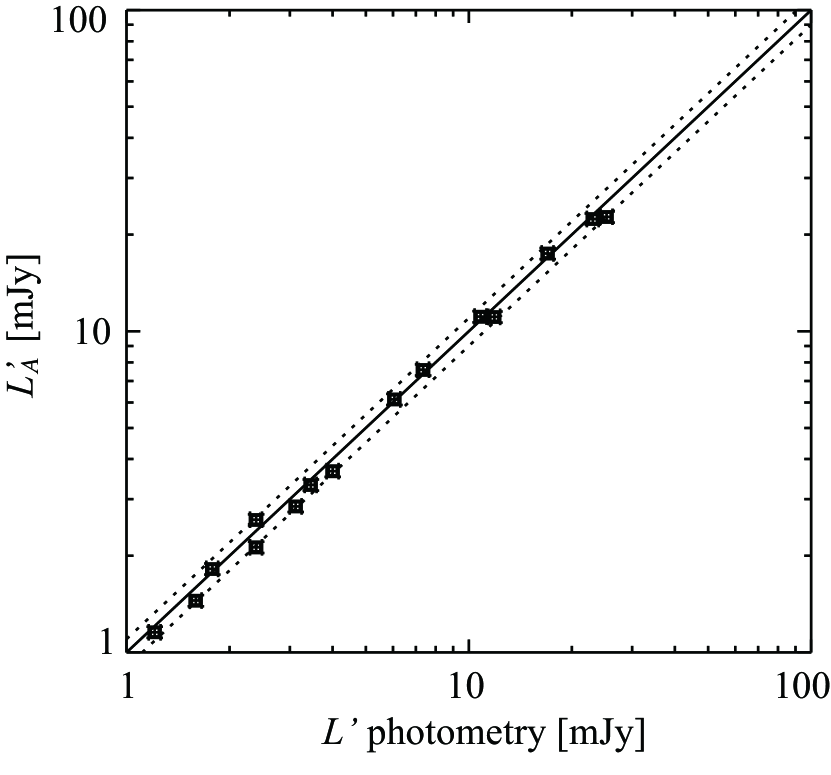
Figure 1: The comparison of the $L^{\prime}$ flux from AKARI spectra and $L^{\prime}$ photometry (Leggett et al. 2002a,b; Golimowski et al. 2004). The past $L^{\prime}$ photometric values are converted to $F_{\nu}$ [mJy]. The border of $\pm 10\%$ is denoted by the dotted lines. We see that the $L^{\prime}$ fluxes from AKARI data are consistent with past $L^{\prime}$ photometry to within 10 $\%$.

3 The 2.5 – 5.0 $\mu$m Spectral Dataset of Brown Dwarfs

Figure 2 shows the spectra of the brown dwarfs in the sequence of their spectral types from L (left bottom) to T (right top).

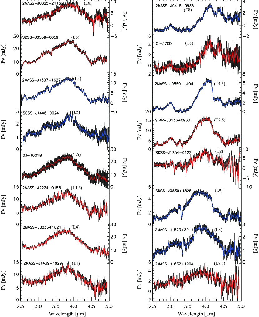
Figure 2: AKARI spectra of 11 L-dwarfs and 5 T-dwarfs. Data taken in Phase 2 are shown as the blue line and these in Phase 3 are drawn in red. The Phase 2 data are generally of better quality than the Phase 3 data. The CO 4.6 $\mu$m band appears in the spectra of all spectral types. The $\mathrm{CH_{4}}$ 3.3 $\mu$m fundamental band appears in the spectra later than L5. The band is seen in SDSS J0539–0059 and 2MASS J1507–1627, but not in the other two L5 sources, GJ 1001B and SDSS J1446+0024. The $\mathrm{CO_{2}}$ absorption band at 4.2 $\mu$m presents in the spectra of late-L and T type dwarfs. The band appear clearly in the spectra of 2MASS J0825+2115 (L6) and SDSS J0830+4828 (L9), but not in the spectrum of 2MASS J1523+3014(L8).

The following molecular absorption bands are clearly recognized in the AKARI data; $\mathrm{H_{2}O}$ (broad absorption bands around 2.7 $\mu$m and at longer than 4.0 $\mu$m), CO (4.6 $\mu$m), $\mathrm{CO_{2}}$ (4.2 $\mu$m), and $\mathrm{CH_{4}}$ (3.3 $\mu$m). Figure 2 shows identification of these bands in the AKARI spectra. The AKARI spectra of L-type dwarfs are gently peaking at 3.8 $\mu$m, and are rather smooth and featureless with the current resolution throughout 2.5–5.0 $\mu$m except for the positions of H₂O and CO. $\mathrm{CH_{4}}$ at 3.3 $\mu$m exists in the dwarfs later than L5. On the other hand, the spectra of T-type dwarfs exhibit deep molecular absorption features further to the broad H₂O bands and CO band.

3.1 CO Absorption Band at 4.6 $\mu$m

Under the assumption of LTE, CO is expected to disappear from the spectra of the late-T type dwarfs because carbon resides mostly in $\mathrm{CH_{4}}$ rather than in CO in a very cool and high-density (T$\sim$1000 K, log $P_{g}$ $\sim$ 6.0 dyn cm^-2) environment (Tsuji 1964). Only few brown dwarf spectra have been obtained in the $M$ band wavelength range (Noll et al. 1997; Oppenheimer et al. 1998; Geballe et al. 2009). They all showed the detections of the CO absorption band in the spectra of mid- to late-T dwarfs. These results raised a very important problem regarding the physics and chemistry of brown dwarf atmospheres. However, due to disturbance caused by the Earth’s atmosphere the quality of these data was not sufficient and the wavelength coverage was limited. Thus detailed analysis of these bands was not easy.

We have obtained much better spectra covering broader range including the CO band with AKARI. The AKARI data show that CO appears in the all observed brown dwarf spectra from early-L to late-T type. We confirm that the spectra of our T-type brown dwarfs clearly exhibit CO absorption band, supporting the previous ground-based studies. It is now clear that the presence of CO in the late-T dwarfs is a common characteristic. It has been argued that CO in the photosphere of late-T dwarfs is maintained by vertical mixing (Griffith & Yelle 1999; Saumon et al. 2000; Yamamura et al. 2010). The vertical mixing transfers CO molecules from the inner regions, where CO is still abundant, to outer cooler regions in the photosphere. However this mechanism does not fully explain the observed strength of the CO band, especially for the late-L to early-T dwarfs (Yamamura et al. 2010). In this paper we do not discuss the strength of CO band any more.

3.2 $\mathrm{CO_{2}}$ Absorption Band at 4.2 $\mu$m

AKARI detected $\mathrm{CO_{2}}$ absorption band at 4.2 $\mu$m in the spectra of brown dwarfs. The band is recognized in all T dwarfs and some late-L dwarfs. We see the band in the spectra of 2MASS J0825+2115 (L6) and SDSS J0830+4828 (L9) clearly, but not in the spectra of 2MASS J1523+3014(L8).

We investigate which spectral types of objects show the $\mathrm{CO_{2}}$ band. Figure 3(a) shows the variation of partial pressure of $\mathrm{CO_{2}}$ for different effective temperatures ($T_{\rm{eff}}$) in the models under the LTE assumption. We see that the partial pressure of $\mathrm{CO_{2}}$ increases with decreasing $T_{\rm{eff}}$ from 2600 to 1600 K, then changes to a decreasing trend with decreasing $T_{\rm{eff}}$ from 1600 to 700 K. This indicates that $\mathrm{CO_{2}}$ is the most abundant in a photosphere with $T_{\rm{eff}}$ $\sim$1600 K. Thus the $\mathrm{CO_{2}}$ absorption band should appear in spectra from L6 to early T dwarfs. However, $\mathrm{CO_{2}}$ 4.2 $\mu$m absorption band does not appear in some observed spectra of late-L to early-T. This analysis tells us that the behavior of $\mathrm{CO_{2}}$ absorption at late-L to early-T dwarfs is very complicated. It may reflect the difference in the elemental abundances (Tsuji et al. 2011, Sorahana et al. in prep.). However, the appearance of $\mathrm{CO_{2}}$ absorption band for late-T dwarfs can not be explained.

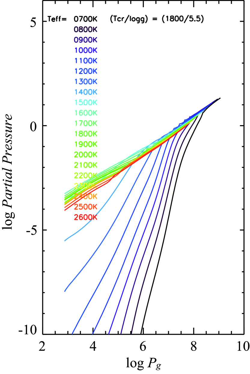
Figure 3: Partial pressures of $\mathrm{CO_{2}}$ molecule for different $T_{\rm{eff}}$ are plotted against total gas pressure. $\mathrm{CO_{2}}$ partial pressure in photosphere has a peak at $T_{\rm{eff}}$=1600 K.

3.3 $\mathrm{CH_{4}}$ Absorption Band at 3.3 $\mu$m

It is known that the $\mathrm{CH_{4}}$ $\nu_{3}$ absorption band at 3.3 $\mu$m already appears in the spectra of a mid-L dwarf (Noll et al. 2000), but the $\mathrm{CH_{4}}$ $\nu_{2}+\nu_{3}$ absorption band at 2.2 $\mu$m which is used for classification of T-type dwarfs, was not detected in the spectra of the same L dwarf (Nakajima et al. 2004). The AKARI data including 3.3 $\mu$m region should enhance our understanding of the CH₄ molecule in the photospheres of L dwarfs. We find that the $\mathrm{CH_{4}}$ 3.3 $\mu$m fundamental band appears in the spectra of brown dwarfs later than L5. Interestingly, we see the band in only two sources out of four L5 dwarfs in our AKARI sample. The band is seen in SDSS J0539–0059 and 2MASS J1507–1627, but not in the other two L5 sources, SDSS J1446+0024 and GJ 1001B (Figure 2).

3.3.1 Equivalent Width of the CH₄ Absorption Band

We examine the appearance of the CH₄ band quantitatively in the AKARI spectra from L1 to L9 dwarfs to confirm this result in detail. In L dwarfs the $\mathrm{CH_{4}}$ band is still weak and only the Q-branch feature is prominent. We derive the equivalent width of the 3.3 $\mu$m CH₄ Q-branch feature in each spectrum, and calculated the ratio between the equivalent width and its uncertainty derived from the standard deviation of the data in the nearby off-feature wavelengths. We evaluate $``$$\mathrm{CH_{4}}$ index$"$ $B_{\mathrm{CH_{4}}}$ as below.

$$B_{\mathrm{CH_{4}}}=\frac{EW}{\left(\frac{\sigma}{F_{\mathrm{center}}}\times d\lambda\times\sqrt{N-1}\right)},$$ (1)

where EW is the equivalent width, $\sigma$ is the standard deviation in the off-band wavelengths, $F_{\mathrm{center}}$ is the estimated flux at the wavelength of the band center derived by linear interpolation from the off-feature region fluxes, $d\lambda$ is the wavelength grid interval and $N$ ($\sim$ 20) is the number of data points within the defined region. We show the results in Table 5 and Figure 4. We regard the detection to be significant when $B_{\mathrm{CH_{4}}}$ is larger than 5. This threshold is chosen because of the following reasons; the $B_{\mathrm{CH_{4}}}$ of the L7.5 dwarfs where the $\mathrm{CH_{4}}$ band is confirmed by eye is 5.25. For L1 and L4 dwarfs where the band is not confirmed are 4.19 and 4.24, respectively. We find that the $\mathrm{CH_{4}}$ 3.3 $\mu$m Q-branch feature starts appearing at L5 type, and the band appears in only two of four L5 dwarfs, SDSS J0539–0059 and 2MASS J1507–1627. The detection of the $\mathrm{CH_{4}}$ absorption band in the spectra of 2MASS J1507–1627 is consistent with the past result reported by Noll et al. (2000).

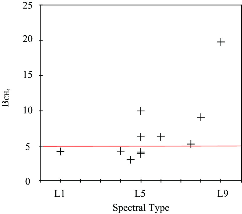
Figure 4: $\mathrm{CH_{4}}$ index $B_{\mathrm{CH_{4}}}$ measured on the AKARI spectra is plotted versus spectral type. $B_{\mathrm{CH_{4}}}$ is ratio of the equivalent width of $\mathrm{CH_{4}}$ Q-branch to its uncertainty from the standard deviation of the data points in the nearby off-band wavelengths. It is found that the onset of the $\mathrm{CH_{4}}$ feature is L5-type dwarfs. The red line indicates the threshold of $\mathrm{CH_{4}}$ detection.

Table 5: The $\mathrm{CH_{4}}$ index for L dwarfs.

Object Name	Sp. Type	$B_{\mathrm{CH_{4}}}$
2MASS J1439+1929	L1	4.12
2MASS J0036+1821	L4	4.24
2MASS J2224–0158	L4.5	3.03
GJ 1001B	L5	3.86
SDSS J1446+0024	L5	4.11
SDSS J0539–00590	L5	9.95
2MASS J1507–1627	L5	6.26
2MASS J0825+2115	L6	6.27
2MASS J1632+1904	L7.5	5.25
2MASS J1523+3014	L8	9.06
SDSS J0830+4828	L9	19.78

Note. — We define the detection threshold as 5.0.

3.3.2 Color index [3.3]–$L^{\prime}_{A}$

$B_{\mathrm{CH_{4}}}$ used in the previous section is only applicable for L-type dwarfs. The $\mathrm{CH_{4}}$ absorption band in T-type spectra becomes broader and deeper, and P- and R- branches are not negligible any more. In order to follow the variation of the $\mathrm{CH_{4}}$ 3.3 $\mu$m absorption in the spectra of brown dwarfs including T-type, we define a photometry band [3.3], which is measured by simply averaging the flux between 3.27 and 3.36 $\mu$m. [3.3]–$L^{\prime}_{A}$ are listed in Table 4, and plotted against the spectral types in Figure 5. The large error of the color for late-T type sources is caused by lack of valid data points around 3.3 $\mu$m in the AKARI spectra due to heavy $\mathrm{CH_{4}}$ absorption. [3.3]–$L^{\prime}_{A}$ colors of early-L dwarfs do not change because $\mathrm{CH_{4}}$ absorption band at 3.3 $\mu$m does not appear in these cases. The [3.3]–$L^{\prime}_{A}$ increases monotonically along L to T sequence, indicating that the $\mathrm{CH_{4}}$ $\nu_{3}$ absorption develops simply toward the later spectral types.

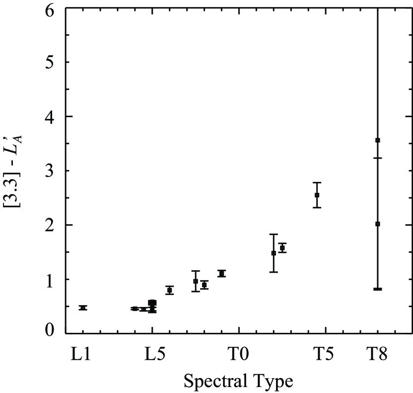
Figure 5: [3.3]–$L^{\prime}_{A}$ color as a function of spectral class. Whereas the colors of early type dwarfs do not change, the color of later than L5 dwarfs tend increasing. This indicates that the $\mathrm{CH_{4}}$ absorption band at 3.3 $\mu$m becomes stronger toward late spectral types.

3.3.3 $J-K$ color

Next, the effects of dust on the observed $\mathrm{CH_{4}}$ band strength are evaluated. The $J$ band flux is the most sensitive to dust extinction. Thus the $J-K$ color would give information of the conditions of dust in the L dwarf photospheres. $K$ photometric values are obtained from Leggett et al. (2000, 2001, 2002a, 2002b) and Knapp et al. (2004). $J-K$ colors are shown in Table 4. We see a trend of redder colors from L1 to L6. Thereafter, $J-K$ colors become bluer later than L6. The red color of early- to mid-L dwarfs is thought be due to increasing dust extinction at $J$ band. We find that the $J-K$ colors of two L5 dwarfs showing the $\mathrm{CH_{4}}$ $\nu_{3}$ absorption band, 2MASS J1507–1627 and SDSS J0539–0059, are bluer than that of other L5 objects without the band, SDSS J1446+0024 and GJ 1001B. This indicates that the difference in L5 dwarfs with or without $\mathrm{CH_{4}}$ $\nu_{3}$ absorption band is caused by dust reddening.

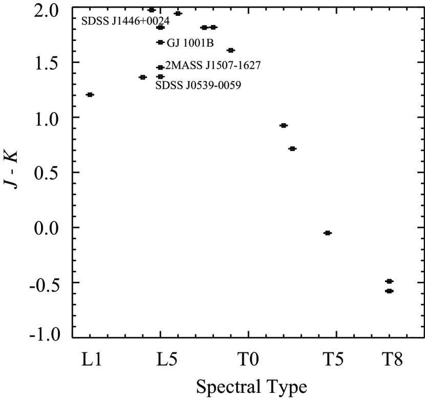
Figure 6: $J-K$ color for objects observed by AKARI. The color becomes redder from early- L to late-L dwarfs. The color from late-L to late-T becomes bluer.

4 Interpretation with the UCM

4.1 The Unified Cloudy Model

To understand the atmospheres of brown dwarfs better, we analyze the AKARI spectra using the Unified Cloudy Model (UCM, Tsuji 2002, 2005). The atmospheres of cool stars are dominated by molecules. The UCM calculates molecular abundance by assuming LTE. Generally, stellar spectra can be interpreted in terms of effective temperature $T_{\rm{eff}}$, surface gravity log g, chemical composition, and micro-turbulent velocity. Dust is an essential component in the atmospheres of brown dwarfs. We assume metallic iron, enstatite (MgSiO₃) and corundum (Al₂O₃) in the UCM as the dust species. Under the LTE dust forms at a layer where temperature drops down to the condensation temperature, $T_{\rm{cond}}$. Although we do not know the exact physics behind the behavior of dust layers, comparison with observations tells that it is difficult to explain the spectra with only these four basic parameters. The UCM assumes that the dust disappears at somewhat lower temperatures given as an additional parameter, namely the critical temperature $T_{\rm{cr}}$. Thus the dust would exist only in the layer with $T_{\rm{cr}}<T<T_{\rm{cond}}$. $T_{\rm{cr}}$ is not predictable by any physical theory at present and is required to be determined from observations empirically. The UCM apply the CH₄ line list by Freedman et al. (2008), which is based on the Spherical Top Data System (STDS) model of Wenger & Champion (1998) and believed to be the best one currently available for this band. Other line lists are CO (Guelachivili et al. 1983, Chackerian & Tipping 1983), $\mathrm{CO_{2}}$ (HITEMP database; Rothman 1997) and $\mathrm{H_{2}O}$ (Partridge & Schwenke 1997). See Tsuji (2002, 2005) for details of the model. We assume that the objects have solar metallicity (here we take the values provided by Allende Prieto et al. 2002) and that the micro turbulent velocity is near the solar value (1km/s) throughout. Then the major parameters that characterize the spectra are $T_{\rm{eff}}$, log g and $T_{\rm{cr}}$.

The two plots in Figures 7 show examples of the models corresponding to L and T dwarf with the parameters ($T_{\rm{cr}}$/log g/$T_{\rm{eff}}$)=(1800 K/5.5/1900 K) and (1900 K/4.5/1200 K), respectively. These figures show profiles of molecular abundances along the position in the photosphere. The abundances change according to the difference of $T_{\rm{eff}}$. We see that CO abundance in the photosphere of the T-type dwarf is significantly smaller than in the L-type photosphere, and instead $\mathrm{CH_{4}}$ becomes the major ingredient. We also show the dust layer ($T_{\rm{cr}}<T<T_{\rm{cond}}$) in Figures 7. We see that the dust layer is located deeper in typical T dwarf photospheres than those in typical L dwarf photospheres. The dust in L dwarf photospheres exists in smaller Rosseland mean tau region than those in T dwarf photospheres, thus the dust affects an L-type spectrum more than a T-type spectrum.

To fit the AKARI spectra, we examine the cases of 700 $\leq$ $T_{\rm{eff}}$ $\leq$ 2200 K in 100 K grid, log g=4.5, 5.0 and 5.5, $T_{\rm{cr}}$=1700, 1800, 1900 K and $T_{\rm{cond}}$ (no dust layer), i.e. a total of 16 $\times$ 3 $\times$ 4 = 192 cases.

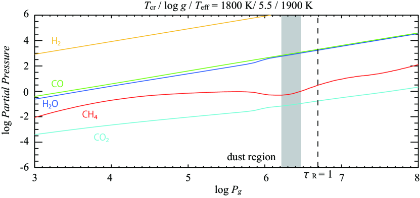
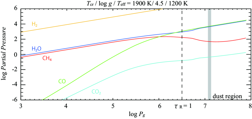
Figure 7: Partial pressures of major molecules in the photospheres of brown dwarfs are plotted against total gas pressure. The model shown in the upper panel is with parameters of ($T_{\rm{cr}}$/log g/$T_{\rm{eff}}$)=(1800 K/5.5/1900 K) corresponding to a L4 type. The lower panel is the model for ($T_{\rm{cr}}$/log g/$T_{\rm{eff}}$)=(1900 K/4.5/1200 K) corresponding to a T5. The dust layer is indicated in gray color. We see that the CO abundance in T5 photosphere is rapidly decreasing toward the surface, log $P_{g}\sim 3.0$ dyn cm^-2, and $\mathrm{CH_{4}}$ takes over the position of the most abundant carbon containing molecule.

4.2 Fitting evaluation

Our purpose of this analysis is to derive the most probable physical parameters for the AKARI sample. The wavelength region of the AKARI data gives us information about $\mathrm{CH_{4}}$, CO and $\mathrm{CO_{2}}$ molecules in the brown dwarf photospheres, and reflects the photospheric temperature relatively free from dust extinction. We use the AKARI spectral data principally to derive the physical parameters via model fitting, but there are some technical hurdles to overcome, as discussed below. Thus we use the shorter wavelength spectra (IRTF/SpeX and UKIRT/CGS4 data) to supplement our analysis. In this section we introduce the shorter wavelength spectra firstly. Then we explain the problem on model fitting and the fitting strategy to overcome the problem.

4.2.1 IRTF/SpeX data

The NASA Infrared Telescope Facility (IRTF) on Mauna Kea, Hawaii, is a 3.0 meter telescope optimized for infrared observations. SpeX is a medium-resolution spectrograph covering 0.8–5.4 $\mu$m on board IRTF. The superiority of SpeX is the capability to provide maximum simultaneous wavelength coverage. A high throughput prism mode that uses single order long slit (60 arcsec) provides the spectral resolution $\lambda/\Delta\lambda=R\sim$ 100 for 0.8–2.5 $\mu$m. Using prism cross-dispersers (for 15 arcsec-long slits), $R$ becomes 1000–2000 across 0.8–2.4 $\mu$m, 2.0–4.1 $\mu$m, and 2.3–5.5 $\mu$m.

Almost all brown dwarfs in our samples have been observed by Burgasser et al. (2004, 2006, 2008, 2010), Burgasser (2007) and Cushing (2004) with SpeX. Nine data sets have been obtained using its low-resolution prism-dispersed mode with resolutions of 75–200 depending on the used slit-width. For these nine objects, we retrieve the data from The SpeX Prism Spectral Libraries built by Adam Burgasser. Only SDSS J0539–0059 was unpublished and the data were obtained from Michael Cushing (private communication). Six other sources have been observed by SpeX using its short wavelength cross-dispersed mode with resolutions of 1200–2000, depending on the used slit-width. We obtained these data from the IRTF Spectral Library maintained by Michael Cushing.

4.2.2 UKIRT/CGS4 data

SDSS J1446+0024 has not been observed with SpeX. A spectrum in 1.0–2.5 $\mu$m was obtained with UKIRT/CGS4 (Geballe et al. 2002). CGS4 is a 1.0–5.0 $\mu$m multi-purpose grating spectrometer which was mounted on the 3.8 m United Kingdom Infrared Telescope (UKIRT), which is sited on Mauna Kea, Hawaii. CGS4 has four gratings. The data of SDSS J1446+0024 were obtained using 40 line/mm grating that provided the resolution of 300–2000, which are defined by 400 $\times$ $\lambda$. The wavelength coverage of this observation is 1.03–1.34 $\mu$m and 1.43–2.53 $\mu$m. We obtained the spectral data of SDSS J1446+0024 from Dagny Looper (private communication).

4.2.3 Absolute Flux Calibration of Short Wavelength Spectral Data

Since nine SpeX data of AKARI samples are normalized at 1.25 $\mu$m, we calibrate their absolute fluxes using the $J$ band photometric data (hereafter $J_{\mathrm{p}}$) given by Leggett et al. (2002a) and Knapp et al. (2004) listed in Table 4. These $J_{\mathrm{p}}$ were taken with the MKO filter. SIMP J0136+0933 was not observed with the MKO filter, and we use 2MASS $J$ band photometric data (Cutri et al. 2003) for the flux calibration of this object. The 2MASS $J$ band magnitude is also listed in 8th-column of Table 4. We estimate the $J$ band flux from SpeX data ($J_{\mathrm{SpeX}}$) with the MKO or 2MASS $J$ band filter transmission function $T$ by calculating equation (2),

$$J_{\mathrm{SpeX}}=\frac{\sum F_{\nu}T(\nu)\Delta\nu}{\sum T(\nu)\Delta\nu}.$$ (2)

After that, we scale the absolute flux of SpeX spectral data with the ratio of $J_{\mathrm{p}}/J_{\mathrm{SpeX}}$.

The absolute flux levels of six objects observed by SpeX and one object observed by the UKIRT/CGS4 were calibrated with the 2MASS $J$ band photometry data by Cushing et al. (2004) and Geballe et al. (2002), respectively. We derive the $J$ band flux from the calibrated spectra to compare with $J_{\mathrm{p}}$ from Leggett et al. (2002a) and Knapp et al. (2004). They are confirmed to be consistent within 10$\%$. Figure 8 shows the results.

The spectra of three objects, 2MASS J1439+1929, 2MASS J0036+1821 and 2MASS J1507–1627, were observed by SpeX in 0.81–4.11 $\mu$m simultaneously with a gap over 2.53–2.85 $\mu$m. They are calibrated by Cushing et al. (2004). In Figure 9 their AKARI spectra and SpeX spectra are plotted in red and black line, respectively. Both AKARI and SpeX data of each object are calibrated independently and scaled by the same factor on the plot. We find that two spectra are consistent within 10 $\%$, which is the uncertainty level of the AKARI spectra.

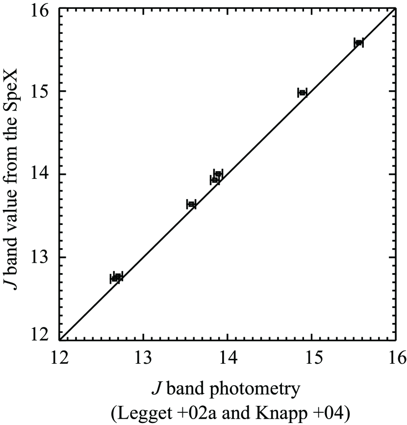
Figure 8: The $J$ band fluxes measured on the IRTF/SpeX and UKIRT/CGS4 spectra are compared with the photometry data by Leggett et al. (2002a) and Knapp et al. (2004). Six SpeX spectra are calibrated by Cushing et al. (2004), and one SGC4 spectrum is by Geballe et al. (2002), respectively. Two measurements of these 7 objects are consistent to within 10 %.

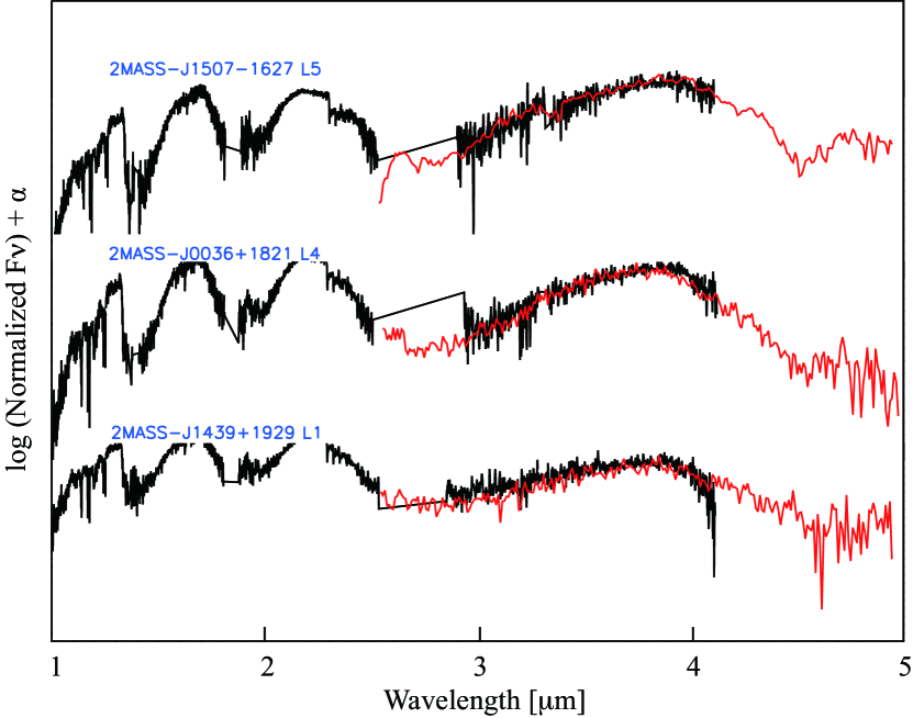
Figure 9: The comparison of SpeX spectral data (black) and AKARI spectra (red) for 2MASS J1439+1929, 2MASS J0036+1821 and 2MASS J1507–1627. Both AKARI and SpeX/CGS4 data of each object are calibrated independently and scaled by the same factor on the plot.

4.2.4 Step1 – Fitting the AKARI Spectra

Our model fitting consists of two processes. As the first step we compare the models with observed AKARI spectra between 2.5 and 4.15 $\mu$m. We use the data only over 2.5–4.15 $\mu$m, not up to 5.0 $\mu$m for fitting, because we know that the current model does not explain the observed spectra beyond 4.15 $\mu$m where the absorption bands of $\mathrm{CO_{2}}$ at 4.2 $\mu$m and CO at 4.6 $\mu$m are present (Yamamura et al. 2010, Tsuji et al. 2011). We follow Cushing et al. (2008) and evaluate the goodness of the model fitting by the statistic G_k, defined as

$$G_{k}=\frac{1}{n-m}\sum_{i=1}^{n}\omega_{i}\left(\frac{f_{i}-C_{k}F_{k,i}}{\sigma_{i}}\right)^{2},$$ (3)

where $n$ is the number of data points; $m$ is degree of freedom (this case $m=3$); $\omega_{i}$ is the weight for the $i$-th wavelength points (we give the weight as $\omega_{i}$ = 1 for all data points because of no bias within each observed spectrum); $f_{i}$ and $F_{k,i}$ are the flux densities of the observed data and $k$-th model, respectively; $\sigma_{i}$ are the errors in the observed flux densities and $C_{k}$ is the scaling factor given by

$$C_{k}=\frac{\sum\omega_{i}f_{i}F_{k,i}/\sigma_{i}^{2}}{\sum\omega_{i}{F_{k,i}}^{2}/{\sigma_{i}}^{2}}.$$ (4)

$G_{k}$ is equivalent to reduced $\chi^{2}$, since we adopt $\omega_{i}$ = 1 in our analysis.

It is difficult to determine a unique best fit model for each AKARI object because of the large error associated with the AKARI spectral data. In general, when the reduced $\chi^{2}$ (=$G_{k}$) is 1–2, the model is regarded to fit the observed data well. However, in our case $G_{k}$ easily falls below unity and we have too many $``$good fit$"$ models. This degeneracy is demonstrated in Figure 10 for the AKARI spectra of 2MASS J1507–1627 (L5). We see that many models have small ($\leq$ 1.04) $G_{k}$ between 1700 to 2000 K of $T_{\rm{eff}}$. The minimum $G_{k}$ is 0.94, and the second minimum is 0.97. The differences of $G_{k}$ between the models near the minimum are too small to determine the best fit model.

Therefore at this step, we select candidates of the best model with the following condition.

$$G_{min}\leq G_{k}<G_{min}+1,$$ (5)

where $G_{min}$ is the minimum $G_{k}$ value. $G_{min}$ is different for every object and is not always near unity, due to the difference in the error of the AKARI observed spectra. We apply $G_{min}$ + 1 as an upper limit. This criterion reasonably selects 5 $\sim$ 20 model candidates for almost all the observed data.

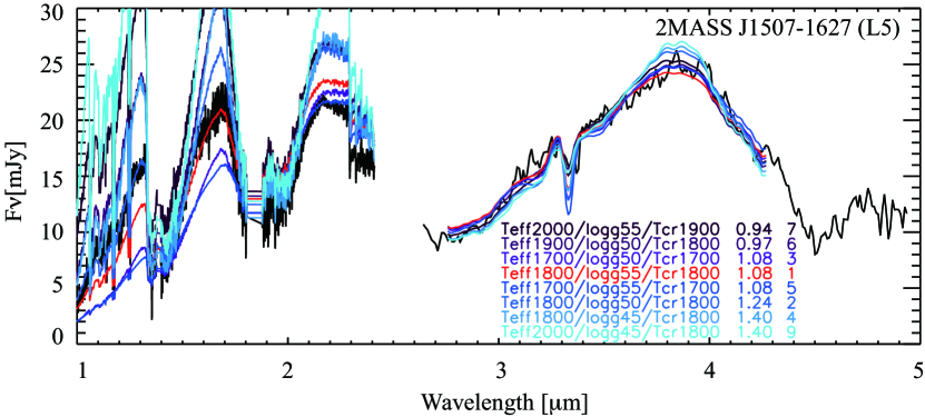
Figure 10: The spectra of 2MASS J1507–1627(L5) and models. The degeneracy in the fitting of AKARI spectrum is solved by adding the SpeX data of the shorter wavelength range. The model spectrum in red color is the best fit model for this object. The order of goodness of the fit to the SpeX data are shown on the right of the legend.

4.2.5 Step2 – Constraining Models with the Short Wavelength Data

To constrain the models from the candidates, we additionally use the spectra in the shorter wavelength range (1.0–2.5 $\mu$m) taken by IRTF/SpeX and UKIRT/CGS4. It is only possible to constrain the model parameter uniquely with the help of the short wavelength range spectra along with the AKARI data. The wavelength region of the AKARI data gives us information about molecules (=gas) in brown dwarf photospheres. On the other hand, data covering shorter wavelengths are the most sensitive to the presence of dust.

We calculate $G_{k}$ for the IRTF/SpeX or UKIRT/CGS4 (hereafter SpeX/CGS4) spectral data for the candidate models derived in Step 1. Since we have validated the absolute flux of the spectra to be accurate to better than 10 $\%$ (see section 2.6), we apply $C_{k}$ values derived in Step 1 (from the AKARI data) to Step 2. Figure 10 shows that the degeneracy appeared in the AKARI wavelengths is resolved in the shorter wavelengths. Results of the model fitting through these processes are shown in Table 6.

We do not fit the AKARI data and the SpeX/CGS4 data simultaneously. This is because the error of two data sets are very different. The average relative error of the AKARI spectra is about 10 $\%$ (Ohyama et al. 2007), while that of the SpeX and CGS4 data is below 0.05 $\%$ (Reyner et al. 2009). This difference would give much higher weight to the SpeX/CGS4 data in the fitting evaluation in Equation (3). Actually, while the reduced $\chi^{2}$ (= $G_{k}$) values of the AKARI data are between 0.1 and 100, those of the SpeX/CGS4 data are between 100 and 5000. Therefore, we decided to use the AKARI spectra first and use the SpeX and CGS4 spectra in the second step.

4.3 Uncertainty of the Model Fitting

Here we discuss the uncertainty of the best fit model parameters. The models we use for the current analysis are calculated on the 100 K (for $T_{\rm{eff}}$ and $T_{\rm{cr}}$) and 0.5 dex (for log g) grid, and the uncertainty should be no better than the grid spacing. To estimate the uncertainty we change one of $T_{\rm{eff}}$, log g and $T_{\rm{cr}}$ by one grid from the best fit value, and search for the $``$restricted best$"$ model by changing other two parameters following the same manner through Step 1 and 2. If we do not find any models satisfying $G_{min}\leq G_{k}<G_{min}+1$ (here $G_{min}$ is taken from the all parameter space in Step 1), the uncertainty of the parameter should be smaller than the grid spacing. When the best parameter is already on the edge of the parameter space; i.e., $T_{\rm{eff}}$ = 700 or 2200 K, log g = 4.5 or 5.5 and $T_{\rm{cr}}$ = 1700 K or $T_{\rm{cond}}$, we only run the test on the available side of the parameter grid.

We show a detailed example for 2MASS J2224–0158 (L4.5), whose best model is ($T_{\rm{cr}}$/log g/$T_{\rm{eff}}$)=(1700 K/5.5/1800 K), in Figure 11. We see large differences in $J$ and $H$ bands in some $``$restricted best$"$ model spectra. We derive a factor to further scale the $``$restricted best$"$ model from that given by $C_{k}$ to adjust the observed spectra in the $J$ and $H$ band region (1.01–1.81 $\mu$m) using Equation 4 (hereafter $C_{J,H}$). We exclude the $``$restricted best$"$ models if the factor, $C_{J,H}$, is more than 1.10 or less than 0.90, regarding the uncertainty of the SpeX/CGS4 absolute flux. For example $C_{J,H}$ for the $``$restricted best$"$ models for $T_{\rm{eff}}$ ($+100$ K and $-100$ K), $T_{\rm{cr}}$ ($+100$ K) and log g ($-0.5$) of 2MASS J2224–0158 (L4.5) are 0.74, 1.12, 0.65, 0.88, respectively. Thus any $``$restricted best$"$ model is invalid for 2MASS J2224–0158 (L4.5), i.e., the uncertainty is smaller than one grid.

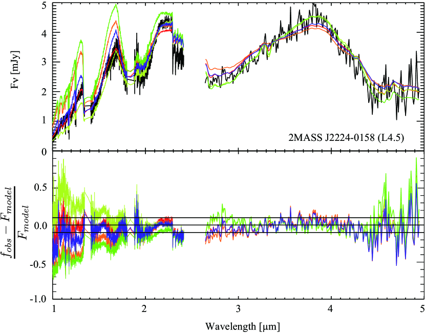
Figure 11: The comparison of the $``$restricted best$"$ models with observed spectrum for 2MASS J2224–0158 (L4.5). The real best fit model is in red and the $``$restricted best$"$ models for $T_{\rm{eff}}$ (+100 K and –100 K), $T_{\rm{cr}}$ (+100 K and –100 K) and log g (+0.5 and –0.5) are in orange, yellow, green, light blue, blue, and purple, respectively. We see that the there are large differences in the $J$ and $H$ bands.

We find that the $``$restricted best$"$ models for the case of changing $T_{\rm{eff}}$ by $\pm$100 K and $T_{\rm{cr}}$ by +100 K exhibit a noticeable change from the real best models. On the other hand, the case of changing $T_{\rm{cr}}$ by –100 K and log g result only in minor differences. We further continue the test of changing each parameter by two grids from the real best fit model. Almost all the $``$restricted best$"$ models do not stay between 0.90 and 1.10 any longer, except for the case of changing two grids of log g. We conclude that our best fit model parameters are determined as good as one grid, and at worst two grids of each parameter for $T_{\rm{eff}}$ and $T_{\rm{cr}}$, but $C_{J,H}$ for the case of changing two grids of log g still stays between 0.90 and 1.10. However, we can not change the grid of log g any more. Therefore the uncertainty of log g is not determined well for some objects. The uncertainties for each object are listed in superscript and subscript in Table 6.

5 Brown Dwarf Atmospheres along with the Spectral Types

5.1 Comparison of the Observed and the Best Fit Model Spectra

The spectra of observed and best fit models are compared in Figure 12. The model spectra generally explain the observed spectral features well, except for some objects noted below. We see that the fit in the entire AKARI region is fairly good, except for the wavelength region longer than 4.15 $\mu$m in mid- to late-T dwarfs, which we do not take into account in the fitting evaluation. We were aware that CO and $\mathrm{CO_{2}}$ bands are not reproduced by the current UCM. Actually, the model fit including this wavelength range makes the fit of the overall AKARI range even worse.

A noticeable deviation is seen in the late-T dwarfs around 3.0 $\mu$m where $\mathrm{H_{2}O}$ and $\mathrm{CH_{4}}$ absorption features overlap. The flux density around the 3.0 $\mu$m region in the model spectra of three late-T dwarfs is too low in comparison to that in the observed spectra. The $\mathrm{CH_{4}}$ absorption at 1.6 $\mu$m in the model spectra of these late-T dwarfs is always significantly weaker than that in the observed spectra. For other brown dwarfs model spectra sometimes do not explain the strength of $\mathrm{CH_{4}}$ $\nu_{3}$ absorption band around 3.3 $\mu$m. We also find that $\mathrm{CO_{2}}$ absorption band in the model of late-L to T dwarfs is sometimes too deep and sometimes too shallow compared to the observations. The fit in the SpeX/CGS4 region is good in an overall sense, except for five late-L and two early-T dwarfs. The $H$ and $K$ band flux density in the model spectra of these five dwarfs are higher than that in the observed spectra.

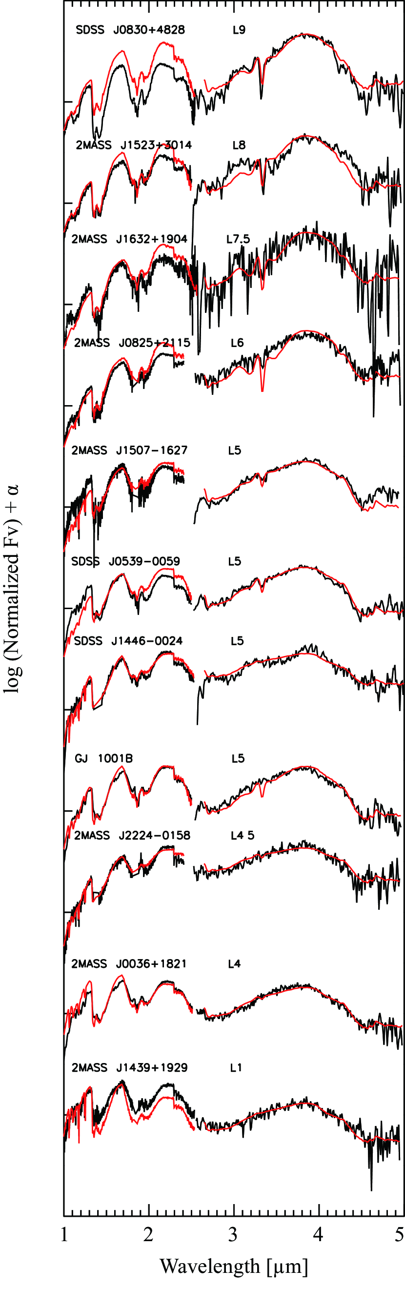
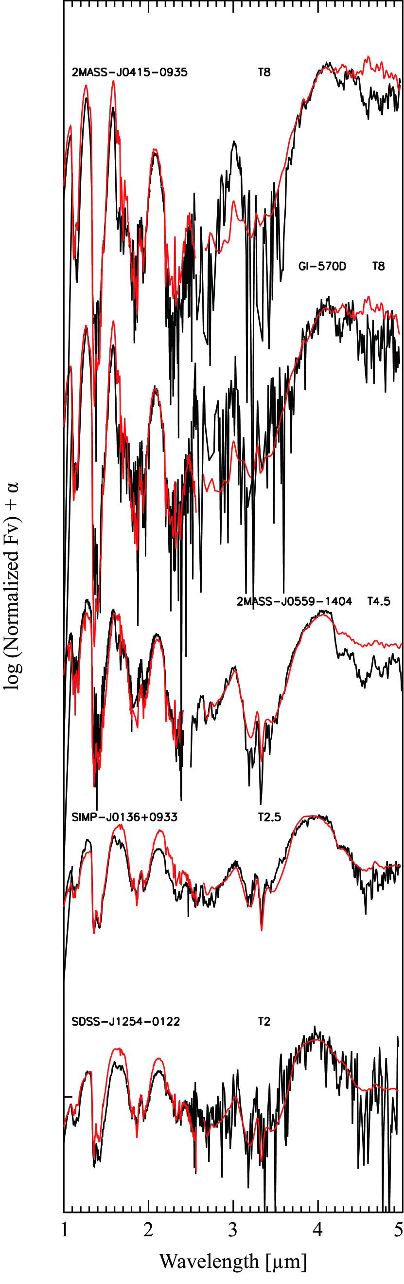
Figure 12: The fitting result. The black lines are the observed data and red lines are the best fit model spectra. The spectra between 2.5 and 5.0 $\mu$m are taken by AKARI and those between 1.0 and 2.5 $\mu$m are taken by IRTF/SpeX (except for SDSS J1446+0024 observed by UKIRT/CGS4).

The high flux level around the 3.0 $\mu$m region in the observed spectra indicates that actual photospheric temperature is higher than that of the models. On the other hand, the result of stronger $\mathrm{CH_{4}}$ absorption band at 1.6 $\mu$m in the observed spectra of late-T dwarfs indicates that the temperature in the photosphere of these dwarfs should be lower than observed. This contradiction implies that the thermal structure of the objects derived by the model is still not perfect. The deviation of the 3.3 $\mu$m $\mathrm{CH_{4}}$ for mid- to late-L dwarfs may also indicate the incompleteness of thermal structure in the model. We have to consider the mechanism to improve the thermal structure to reproduce the observation data. The second possible reason of discrepancy between the model and observations is incompleteness of the line lists. It is known that the line lists of polyatomic molecules, such as $\mathrm{H_{2}O}$, $\mathrm{CH_{4}}$, or $\mathrm{CO_{2}}$, are still not perfect. The effects of line list should be investigated, however it is not likely that these discrepancies are caused only by the incomplete line lists. A third option would be the elemental abundance. The discrepancy of $\mathrm{CO_{2}}$ absorption in the observed spectra may indicate that the elemental abundances in the photospheres of these objects are different from the assumptions in the model. Excess of $\mathrm{CO_{2}}$ absorption of SDSS J0830$+$4828 (L9), 2MASS J0559–1404 (T4.5) and 2MASS J0415–0935 (T8) were discussed by Tsuji et al. (2011) in terms of enhanced C and O elemental abundances. Recently, Madhusudhan et al. (2011) reported an anomaly in the $\mathrm{H_{2}O}$ and $\mathrm{CH_{4}}$ abundances compared to the solar abundance chemical equilibrium model prediction in the atmosphere of the hot-Jupiter WASP-12b. They suggested that the abundance of these molecules can be explained if the carbon-to-oxygen ratio [C]/[O] in this planet’s atmosphere is much greater than the solar value ([C]/[O]=0.54), i.e., [C]/[O]$>1$. Although the structure of atmosphere may be different in planets and brown dwarfs, these results are consistent with our conclusion; the elemental abundance is an essential parameter of brown dwarf / planet atmosphere and should be carefully considered in future studies. We extend the study of possible elemental abundance variations among brown dwarfs using model atmospheres and the AKARI data in a forthcoming paper (Sorahana et al. in prep).

The $H$ and $K$ band flux densities in the model spectra of late-L and early-T dwarfs are always higher than those in the observed spectra. Since the wavelength range of SpeX/CGS4 is the most sensitive to the dust extinction, we can evaluate the dust amount from the spectra of this wavelength region. The effect of dust extinction turned out to be small in the late-L to early-T dwarfs. Less warming up effect by the dust is expected. This argument indicates that an increase of the dust and the inner temperature are overestimated in the models as compared to actual photospheres. Since dust opacity relies on the composition, grain size distribution and amount, we shall confirm the effects of these quantities in the UCM. We also propose that a self-consistent, more realistic theory of condensation and sedimentation in the atmospheres is essential in future brown dwarf atmosphere models.

5.2 Model Parameters and Spectral Type

Parameters of the best fit models are shown in Table 6, and the parameters are plotted in Figure 13 with respect to the spectral types. We see that the spectral types are in principle in the sequence of $T_{\rm{eff}}$ (Figure 13 (a)). $T_{\rm{eff}}$ in late-L dwarfs have approximately the same value. log g shown in Figure 13 (b) appears to be associated with the spectral types, but with large uncertainty as shown in section 4.3. For $T_{\rm{cr}}$ shown in Figure 13 (c), we see a decreasing trend from L1 to L6, then $T_{\rm{cr}}$ changes and increasing for the objects later than L6. The uncertainties of $T_{\rm{cr}}$ of 2MASS J1523+3014 (L8) and SDSS J0830+4828 (L9) are relatively large. For the spectra near the L/T transition it is very difficult to fit the spectra over a wide wavelength range with a model spectrum. Even the best fit model spectrum deviates from observed spectrum in many points. However, the spectral shape of the best fit model agrees with the observed one much better than any $``$restricted best$"$ models by eye, and we are convinced that the best fit model parameters are secure, i.e., $T_{\rm{cr}}$ has a minimum at L6.

The result of almost constant $T_{\rm{eff}}$ in late-L dwarfs has already been pointed out by past studies. Tsuji and Nakajima (2003) argued that little change in $T_{\rm{eff}}$ would be caused by cloud migration from optically thin upper regions to the thick inner regions. We confirm this hypothesis from the derived $T_{\rm{cr}}$ in Figure 13 (c). From our fitting analysis the dust effect appears to become larger from early- to mid-L dwarfs. This result is consistent with the $J-K$ color shown in Figure 6. Mid-L dwarfs should have the largest amount of dust. The trend of $T_{\rm{cr}}$ along their spectral types shows that the contribution of dust to the spectra becomes smaller from late-L dwarfs to late-T dwarfs. Our result attests to the suggestion in Tsuji & Nakajima (2003).

Table 6: Best fit model parameters and their uncertainty derived by fitting the AKARI and the SpeX/CGS4 data.

Object Name	Sp.Type	$T_{\rm{cr}}$[K]	log g	$T_{\rm{eff}}$[K]
2MASS J1439+1929	L1	1800-100	5.5-1.0	2100
2MASS J0036+1821	L4	1800	5.5	2000-100
2MASS J2224–0158	L4.5	1700	5.5	1800
GJ 1001B	L5	1800-100	5.0-0.5	1800
SDSS J1446+0024	L5	1700+100	5.0+0.5	1800
SDSS J0539–0059	L5	1800	5.5	1800
2MASS J1507–1627	L5	1800	5.5-0.5	1800
2MASS J0825+2115	L6	1700	4.5	1500
2MASS J1632+1904	L7.5	1700	4.5+0.5	1500+100
2MASS J1523+3014	L8	1800-100	4.5+1.0	1600${{}^{+100}_{-100}}$
SDSS J0830+4828	L9	1800-100	4.5+0.5	1600-100
SDSS J1254–0122	T2	1800	5.5	1400
SIMP J0136+0933	T2.5	1800-100	4.5+1.0	1400+100
2MASS J0559–1404	T4.5	1900+100	4.5+0.5	1200+100
Gl 570D	T8	2000	4.5	700
2MASS J0415–0935	T8	2000	4.5	700

Note. — The upper and lower uncertainties for each object are shown in the superscript and subscript, respectively.

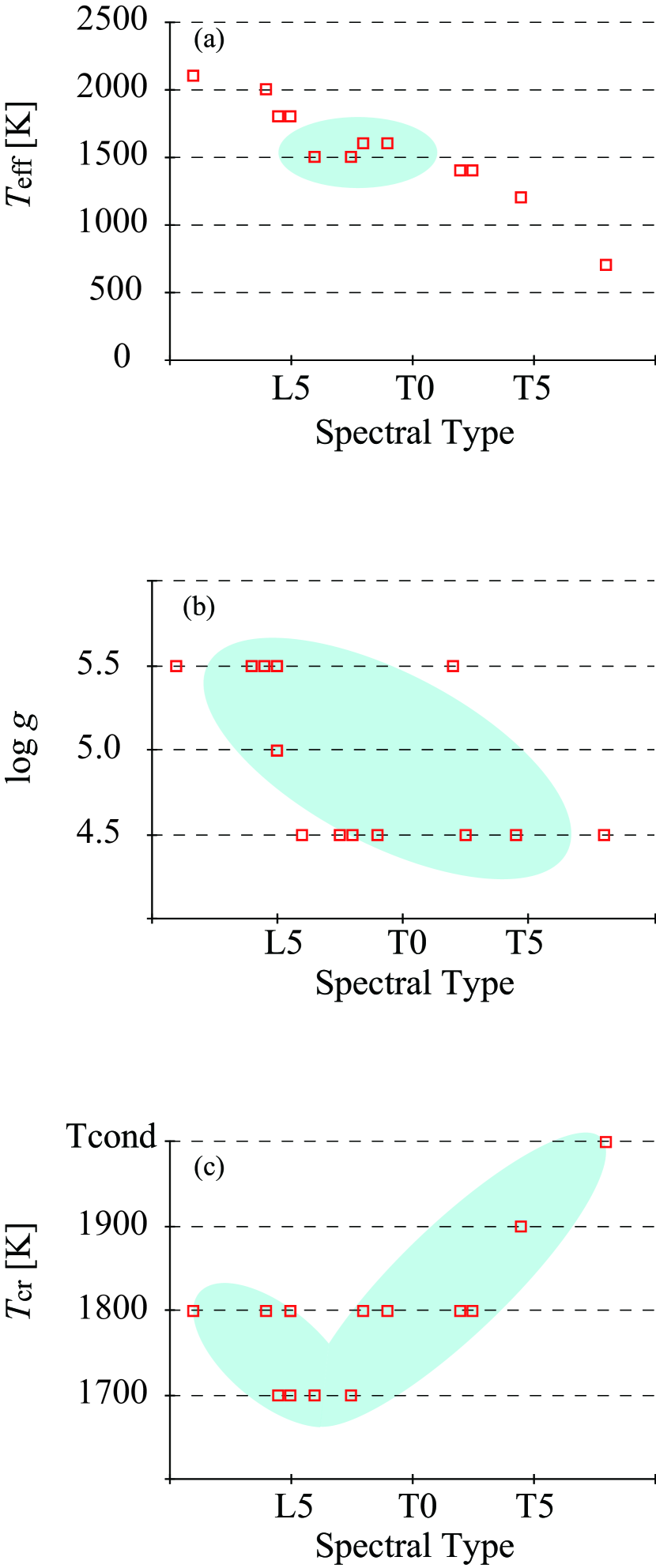
Figure 13: The best fit model parameters versus spectral type, (a) $T_{\rm{eff}}$, (b) log g, and (c) $T_{\rm{cr}}$. Objects with the same spectral type may overlap when they have the same parameters. We see that spectral type is in the sequence of $T_{\rm{eff}}$ except for the late-L dwarfs. log g decreases toward the late spectral types. $T_{\rm{cr}}$ is minimum for mid- to late-L types.

5.3 Advantage of AKARI Spectra to the Model Fitting

In previous studies, physical parameters of brown dwarfs have been derived mainly from near-infrared (1.0–2.5 $\mu$m) spectra. Tsuji et al. (2004) attempted to interpret the near-infrared spectra (0.882–1.400 $\mu$m, 1.056–1.816 $\mu$m, and 1.850–2.512 $\mu$m) obtained with Subaru Telescope with the UCM. They reported that the overall SEDs and the strengths of the major spectral features are reasonably, but not perfectly, reproduced by the UCM. In their fitting, dust extinction effects (most effectively contributing to $J$ and $H$ band) and molecular band strengths were the key features in determining the physical parameters from model candidates, but it is hardly realized that these features are all consistent with an observation. They commented that it was difficult to derive reliable physical parameters for each object by the UCM even though their fitting to the near-infrared spectra (only) can constrain the physical parameters in a certain range.

The spectra in 2.5–5.0 $\mu$m obtained by AKARI should provide additional information on brown dwarf atmospheres, as the fundamental bands of major molecules, $\mathrm{H_{2}O}$, CO, $\mathrm{CO_{2}}$ and $\mathrm{CH_{4}}$ are located in this region with less effects of dust opacity. These molecular bands may sample different part of the photosphere. By including the AKARI spectra into the model analysis, we expect to improve the model fitting to reflect more global characteristics of the objects. Cushing et al. (2008) also mentioned that the model fitting to the broader wavelength range results in more reliable physical parameters, even though the fits to the narrower wavelength region can be better.

To demonstrate the benefit of the AKARI spectra, we compare the observed spectra of two brown dwarfs, 2MASS J1523$+$3014 (L8)and SDSS J1254$--$0122 (T2), with the models derived by the current study and by Tsuji et al. (2004) in Figure 14. We see that both model spectra reasonably reproduce the near-infrared part of the observed spectra. However, the AKARI spectra can be explained only with our models.

This result indicates that the parameters derived only from near-infrared spectra might have large uncertainties, and the broader wavelength data including AKARI spectra are essential to understand the nature of brown dwarf atmospheres. We find that $T_{\rm{eff}}$ derived by our model fitting is generally $\sim$100 K higher than that of Tsuji et al. (2004) for the same spectral type objects. It is probably because of the fact that molecular bands in the AKARI wavelength range help to distinguish between the effects of $T_{\rm{eff}}$ and $T_{\rm{cr}}$.

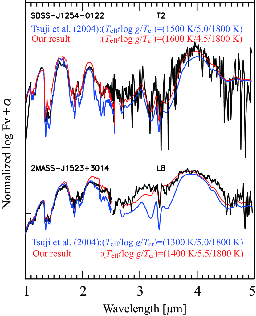
Figure 14: The best fit model spectrum in the current study (red) and that from Tsuji et al. (2004) (blue) are compared with the AKARI+SpeX observed spectra (black) of two brown dwarfs, 2MASS J1523+3014 and SDSS J1254–0122. It is seen that the near-infrared part ($\leq 2.5$ $\mu$m) is reasonably well reproduced by both the models, but AKARI spectra at longer wavelength is much better explained by the current model, showing that the AKARI spectra give further constraint to the model parameters.

6 Conclusion

We study the presence of 4.6 $\mu$m CO, 4.2 $\mu$m CO₂ and 3.3 $\mu$m CH₄ bands in 16 AKARI brown dwarf spectra over the wide range of spectral types. We confirm that the CH₄ band appears in the sources as early as L5, and find that the band is seen in only two of four L5 dwarfs in our sample. Their $J-K$ color indicates that the appearance of $\mathrm{CH_{4}}$ band in two L5 dwarfs is related to the dust abundance. The CO 4.6 $\mu$m band appears in the spectra of all spectral types until late-T dwarfs. The fact that CO generally exists in all brown dwarf atmospheres is very important, since it is confirmed that the deviation of molecular abundance in brown dwarf atmospheres from the LTE prediction is a common feature. We need further consideration on this problem in future works. We detect $\mathrm{CO_{2}}$ absorption band at 4.2 $\mu$m in the spectra of late-L and T type dwarfs. These detections indicate that the $\mathrm{CO_{2}}$ molecule is generally in the atmospheres of these dwarfs.

We analyze the AKARI spectra using the UCM. We derive the three physical parameters, effective temperature $T_{\rm{eff}}$, critical temperature $T_{\rm{cr}}$, and surface gravity log g, of 16 sources by systematic model fitting. We investigate how the spectral type correlate with the parameters. We find that the spectral type follows a sequence of $T_{\rm{eff}}$, except for the late-L dwarfs, for which the spectral type is a sequence of $T_{\rm{cr}}$, the parameter related to the effects of dust. This result confirms expectations from past studies. AKARI give us these new insights on brown dwarf atmospheres in the new spectral range, 2.5–5.0 $\mu$m. We also find important problems, which are not explained with the current brown dwarf atmosphere model. Therefore, the models need improvements and the AKARI spectra should be analyzed in further detail.

We thank to the anonymous referee for critical reading of our manuscript and constructive suggestions. We are grateful to Dr. Poshak Gandhi for his careful checking our manuscript and suggestions to improve the text. This research is based on observations with AKARI, a JAXA project with the participation of ESA. We thank Prof. Takashi Tsuji for his kind permission to access the UCM and for helpful suggestions. Dr. Adam Burgasser, Dr. Michael. Cushing, and Dr. Dagny. Looper generously provided me (Sorahana) observed data, along with warm encouragement. We acknowledge JSPS (PI: S. Sorahana) and JSPS/KAKENHI(c) No. 22540260 (PI: I. Yamamura).

References

- Allende Prieto et al. (2002) Allende Prieto, C., Lambert, D. L., & Asplund, M. 2002, ApJ, 573, L137
- Artigau et al. (2008) Artigau, É., Biller, B. A., Wahhaj, Z., et al. 2008, SPIE, 7014, 66
- Burgasser (2007) Burgasser, A. J. 2007, ApJ, 659, 655
- Burgasser et al. (2010) Burgasser, A. J., Cruz, K. L., Cushing, M., et al. 2010, ApJ, 710, 1142
- Burgasser et al. (2006) Burgasser, A. J., Geballe, T. R., Leggett, S. K., Kirkpatrick, J. D., & Golimowski, D. A. 2006, ApJ, 637, 1067
- Burgasser et al. (2008) Burgasser, A. J., Liu, M. C., Ireland, M. J., Cruz, K. L., & Dupuy, T. J. 2008, ApJ, 681, 579
- Burgasser et al. (2004) Burgasser, A. J., McElwain, M. W., Kirkpatrick, J. D., et al. 2004, ApJ, 127, 2856
- Burgasser et al. (2000) Burgasser, A. J., Wilson, J. C., Kirkpatrick, J. D., et al. 2000, AJ, 120, 1100
- Burrows et al. (2001) Burrows, A., Hubbard, W. B., Lunine, J. I., & Liebert, J. 2001, RvMP, 73, 719
- Chackerian & Tipping (1983) Chackerian, C. J., & Tipping, R. H. 1983, J. Mol. Spectrosc., 99, 431
- Cushing (2004) Cushing, M. C. 2004, PhD thesis, Univercity of Hawaii
- Cushing et al. (2008) Cushing, M. C., Marley, M. S., Saumon, D., et al. 2008, ApJ, 678, 1372
- Cushing et al. (2004) Cushing, M. C., Vacca, W. D., & Rayner, J. T. 2004, PASP, 116, 362
- Cutri et al. (2003) Cutri, R. M., Skrutskie, M. F., van Dyk, S., et al. 2003, yCat., 2246, 0
- Dahn et al. (2002) Dahn, C. C., Harris, H. C., Vrba, F. J., et al. 2002, AJ., 124, 1170
- Fegley & Lodders (1996) Fegley, Jr., B., & Lodders, K. 1996, ApJ, 472, L37
- Freedman et al. (2008) Freedman, R. S., Marley, M. S., & Lodders, K. 2008, ApJS, 174, 504
- Geballe et al. (2002) Geballe, T. R., Knapp, G. R., Leggett, S. K., et al. 2002, ApJ, 564, 466
- Geballe et al. (2009) Geballe, T. R., Saumon, D., Golimowski, D. A., et al. 2009, ApJ, 695, 844
- Golimowski et al. (2004) Golimowski, D. A., Leggett, S. K., Marley, M. S., et al. 2004, AJ, 127, 3516
- Griffith & Yelle (1999) Griffith, C. A., & Yelle, R. V. 1999, ApJ, 519, L85
- Guelachivili et al. (1983) Guelachivili, G., De Villeneuve, D., Farrenq, R., Urban, W., & Verges, J. 1983, J. Mol. Spectrosc., 98, 64
- Jameson et al. (2008) Jameson, R. F., Casewell, S. L., Bannister, N. P., et al. 2008, MNRAS, 384, 1399
- Kawada et al. (2007) Kawada, M., Baba, H., Barthel, P. D., et al. 2007, PASJ, 59, 389
- King et al. (2010) King, R. R., McCaughrean, M. J., Homeier, D., et al. 2010, A&A, 510, 99
- Knapp et al. (2004) Knapp, G. R., Leggett, S. K., Fan, X., et al. 2004, AJ, 127, 3553
- Larimer (1967) Larimer, J. W. 1967, GeCoA, 31, 1215
- Larimer & Anders (1967) Larimer, J. W., & Anders, E. 1967, GeCoA, 31, 1239
- Leggett et al. (2001) Leggett, S. K., Allard, F., Geballe, T. R., Hauschildt, P. H., & Schweitzer, A. 2001, ApJ, 548, 908
- Leggett et al. (2000) Leggett, S. K., Geballe, T. R., Fan, X., et al. 2000, ApJ, 536, L35
- Leggett et al. (2002a) Leggett, S. K., Golimowski, D. A., Fan, X., et al. 2002a, ApJ, 564, 452
- Leggett et al. (2002b) Leggett, S. K., Hauschildt, P. H., Allard, F., Geballe, T. R., & Baron, E. 2002b, MNRAS, 332, 78
- Lord (1965) Lord, III, H. C. 1965, lcar, 4, 279
- Lorente et al. (2008) Lorente, N. P. F., Glasse, A. C. H., Ramsay Howat, S. K., & Evans, C. J. 2008, ASPC, 394, 187
- Madhusudhan et al. (2011) Madhusudhan, N., Harrington, J., Stevenson, K. B., et al. 2011, Nature, 469, 64
- Murakami et al. (2007) Murakami, H., Baba, H., Barthel, P., et al. 2007, PASJ, 59, 369
- Nakajima et al. (1995) Nakajima, T., Oppenheimer, B. R., Kulkarni, S. R., et al. 1995, Nature, 378, 463
- Neugebauer et al. (1984) Neugebauer, G., Soifer, B. T., Miley, G., et al. 1984, ApJ, 278, L83
- Noll et al. (2000) Noll, K. S., Geballe, T. R., Leggett, S. K., & Marley, M. S. 2000, ApJ, 541, L75
- Noll et al. (1997) Noll, K. S., Geballe, T. R., & Marley, M. S. 1997, ApJ, 489, L87
- Ohyama et al. (2007) Ohyama, Y., Onaka, T., Matsuhara, H., et al. 2007, PASJ, 59, 411
- Onaka et al. (2007) Onaka, T., Matsuhara, H., Wada, T., et al. 2007, PASJ, 59, 401
- Oppenheimer et al. (1998) Oppenheimer, B. R., Kulkarni, S. R., Matthews, K., & van Kerkwijk, M. H. 1998, ApJ, 502, 932
- Partridge & Schwenke (1997) Partridge, H., & Schwenke, D. W. 1997, J. Chem. Phys., 106, 4618
- Rothman (1997) Rothman, L. S. 1997, High-temperature Molecular Spectroscopic Database (CD-ROM) (Andover: ONTAR Co.)
- Saumon et al. (2000) Saumon, D., Geballe, T. R., Leggett, S. K., et al. 2000, ApJ, 541, 374
- Saumon et al. (2006) Saumon, D., Marley, M. S., Cushing, M. C., et al. 2006, ApJ, 647, 552
- Tsuji (2002) Tsuji, T. 2002, ApJ, 575, 264
- Tsuji (2005) —. 2005, ApJ, 621, 1033
- Tsuji & Nakajima (2003) Tsuji, T., & Nakajima, T. 2003, ApJ, 585, L151
- Tsuji et al. (2004) Tsuji, T., Nakajima, T., & Yanagisawa, K. 2004, ApJ, 607, 511
- Tsuji et al. (2011) Tsuji, T., Yamamura, I., & Sorahana, S. 2011, ApJ, 734, 73
- Vrba et al. (2004) Vrba, F. J., Henden, A. A., Luginbuhl, C. B., et al. 2004, AJ, 127, 2948
- Wenger & Champion (1998) Wenger, C., & Champion, J. P. 1998, J. Quant. Spec. Radiat. Transf., 59, 471
- Yamamura et al. (2010) Yamamura, I., Tsuji, T., & Tanabé, T. 2010, ApJ, 722, 682