Effects of permeability and viscosity in linear polymeric gels

Abstract

We propose and analyze a mathematical model of the mechanics of gels, consisting of the laws of balance of mass and linear momentum. We consider a gel to be an immiscible and incompressible mixture of a nonlinearly elastic polymer and a fluid. The problems that we study are motivated by predictions of the life cycle of body-implantable medical devices. Scaling arguments suggest neglecting inertia terms, and therefore, we consider the quasi-static approximation to the dynamics. We focus on the linearized system about relevant equilibrium solutions, and derive sufficient conditions for the solvability of the time dependent problems. These turn out to be conditions that guarantee local stability of the equilibrium solutions. The fact that some equilibrium solutions of interest are not stress free brings additional challenges to the analysis, and, in particular, to the derivation of the energy law of the systems. It also singles out the special role of the rotations in the analysis. From the point of view of applications, we point out that the conditions that guarantee stability of solutions also provide criteria to select material parameters for devices. The boundary conditions that we consider are of two types, first displacement-traction conditions for the governing equation of the polymer component, and secondly permeability conditions for the fluid equation. We present a rigorous study of these conditions in terms of balance laws of the fluid across the interface between the gel and its environment [20], and use it to justify heuristic permeability formulations found in the literature [39], [14]. We also consider the cases of viscous and inviscid solvent, assume Newtonian dissipation for the polymer component. We establish existence of weak solutions for the different boundary permeability conditions and viscosity assumptions. We present two-dimensional, finite element numerical simulations to study pressure concentration on edges, in connection with the debonding phenomenon between the gel and the boundary substrate upon reaching a critical pressure.

1 Introduction

This article addresses mechanical modeling, stability of equilibrium states and analysis of boundary value problems of quasi-static gel dynamics. We assume that a gel is an incompressible and immiscible mixture of polymer and solvent, and study the coupled system of equations of balance of mass and linear momentum of the components. Boundary conditions are of traction-displacement type together with statements of the permeability of the gel boundary to the environmental fluid. This work is motivated by problems arising in the prediction of the life cycle of body-implantable medical devices.

Gels consist of crosslinked or entangled polymeric networks holding fluid. In its swollen state, the polymer confines the solvent and, in turn, the solvent prevents the gel from collapsing into dry polymer. Gels are abundantly present in nature and occur when materials are placed in a fluid environment. Devices such as pacemakers, bone replacement units and artificial skin turn into gel when implanted in the body. The materials that constitute a device differ in swelling ratio, this causing a build up of stress at the interfaces, as well as at the contact between the device and its boundary support. High stresses, above the manufacturer’s guaranteed threshold, may cause debonding instability leading to device failure.

The equations that we analyze encode relevant properties of gel behavior such as solvent diffusion, transport of polymer and solvent, friction and viscosity, elasticity, and time relaxation. They consist of equations of balance of mass and linear momentum for the polymer and fluid components, together with the saturation (incompressibility) constraint. Assuming that the polymer is an isotropic, elastic solid, the total energy of the gel is the sum of the elastic stored energy function of the polymer and the Flory-Huggins energy of mixing. The variable fields of the equilibrium problem consist of the volume fractions of the gel components and the deformation gradient tensor of the polymer. These fields are not all independent, but they are related by the equation of balance of mass of the polymer and the saturation condition on the gel. The problem of constrained energy minimization studied by Micek, Rognes and Calderer in [26] established sufficient conditions on the energy and on the imposed boundary conditions that guarantee existence of a global energy minimizer. The authors also developed, analyzed and numerically implemented a mixed finite element discretization of the equilibrium linear operator. A challenge of the analysis is the presence of residual stress in the reference configuration of the polymer. The work yielded numerical evaluations of shear stress at the interface between two gels representing bone tissue and the artificial implant. However, gel behavior is inherently a time evolution problem due to the combined effects of transport, diffusion and dissipation. This serves as a motivation to the work presented in this article.

Scaling arguments for gels consisting of polymer melts justify neglecting the inertia terms and analyzing the quasi-static system. Specifically, the size of polymer dissipation effects with respect to inertia results in the latter being dominant at time scales on the order of $10^{-7}$ seconds [9]. Of course, such time scales are negligible for biomedical devices with typical life-cycle of 20 years. From a different perspective, the effect of the inertia terms was analyzed by Zhang and Calderer [9]. They studied the free boundary problem of gel swelling, in one space dimension, neglecting the Newtonian dissipation of the both gel components. In such a case, the governing equation turns out to be a frictional, weakly dissipative, hyperbolic partial differential equation [12], [13]. The scaling that justifies retaining the inertia effects is consistent with the dynamics of polysaccharide gel networks found in many living systems, such as in gliding myxobacteria [22], [30].

The model proposed here shares analogies with deformable porous media flow models but has the additional feature of accounting for interaction between fluid and polymer through the Flory-Huggins energy. From a different perspective, especially challenging multi-component mixtures are used in geology and in oil and natural gas recovery models [3], [4], [28]. In these models, a relevant role is played by the Terzaghi’s stress, which is the pressure exerted by the fluid in the pores against the stress applied to the rock. Its analog in the case of the gel is the pressure in the solvent accounted by the Flory-Huggins energy. The current analysis is not immediately extendable to the triphasic models when one of the components is compressible.

The governing system that we study is motivated by the stress-diffusion coupling model developed by Doi and Yamaue [39], [14], [40], [41], and also by Hong et al. [37]. Feng and He [15] studied purely inviscid gels with impermeable boundary as governed by the stress-diffusion coupling model. Our model treats the polymer component of the gel as a nonlinear elastic solid, and includes, both, fluid and polymer dissipation, diffusion, the Flory-Huggins interaction, and accounts for different permeability properties of the interface between the gel and the surrounding fluid as well as traction-displacement conditions imposed on the polymer boundary. To our knowledge, all these combined effects have not been accounted for in the previous works. We develop an existence theory for the governing system of partial differential equations, linearized about an equilibrium state. Some of the tools presented in [15] have been applied to our analysis, in the case that the solvent is inviscid. One novelty of this work is the derivation of permeability conditions from balance balance laws at the interface between the gel and its surrounding fluid, following a model developed for the treatment of polyelectrolyte gels [20].

We assume that the polymer component of the gel is an isotropic elastic material with Newtonian dissipation. The equations possess bulk, stress free, equilibrium solutions that are pure expansion or compression. We point out that, as for isotropic elasticity, if the energy is convex with respect to the deformation gradient, these are the only stress free critical points. However, if the energy is nonconvex, the system may also admit non-spherical equilibrium deformations. These states may be consistent with experimentally observed pattern structures in polyelectrolyte gels [5], [6] and [29]. Equilibrium gel states with nonzero stress are also relevant in many applications. In particular, reference configurations with residual stress may be counted as a special case of the former. Our analysis, addresses the two types of linearization of the governing system, first, about stress free spherical deformations, and secondly about equilibrium solutions that satisfy mixed traction-displacement boundary conditions. Within this perspective, we may consider the process of device implantation as subjecting an originally stress free body to displacement initial and boundary conditions, as well as to the environmental stress of the surrounding tissue, and the permeability effects of such a contact. The device will no longer be at equilibrium under the newly imposed initial and boundary conditions, and a dynamical process will begin at implantation. The second type of linearization is relevant to the iterative process of solution of a nonlinear problem.

We derive restrictions on the constitutive equations that ensure the coercivity of the static operators. These are also known as the Coleman and Noll conditions and guarantee the classical stability requirement that the stress work be non-negative in every strain ([36], sections 52 and 83). Moreover, we find that the procedure of deriving the energy relation brings out the special role of the rotations in the case that residual stresses are present.

We assume that the reference configuration of the gel is that of the polymer network previous to the gel formation. Accordingly, the boundary of the current domain is that of the polymer, and it evolves with its velocity. The Eulerian formulation of the governing system of the gel and the natural Lagrangian setting of solid elasticity of the polymer present challenges to the analyses. These manifest themselves in the derivation of the energy relations satisfied by weak solutions of the governing systems. We consider the cases of impermeable and fully permeable boundary between the gel and the environmental fluid. The case of a semipermeable gel boundary follows from the former, with some elementary modifications, and so, we omit its presentation. Finally, we point out that the conditions for local equilibria employed in the solvability of the time dependent problems are also sufficient to guarantee regularity of the weak solutions.

In related work, we developed and analyzed a numerical method based on finite elements to simulate solutions of the models presented here, in two dimensional domains, in the case that the fluid is inviscid. We consider a gel sample in the unit square, subject to zero displacement in two opposite edges and to a fixed pressure of $10^{4}Pa$ in the other two. We calculate the stress components under the following criteria: the relative scaling of the Flory-Huggins energy with respect to the elastic one, the degree of stiffness, expansion and compressibility of the polymer, and the type of boundary permeability. The elasticity modulus of the polymer is set at $1$GPa, consistent with values encountered in device materials. We find that pressure concentrates on the edges where the the displacement is held to zero, its values increasing with decreased compressibility, and large stiffness. Permeability also promotes stress concentration, but with the interior stress being lower than that in the impermeable case. If the pressure at an edge overcomes the debonding threshold, then it would detach from its support. The experimental literature reports on values of the debonding pressure for different materials ranging from 0.5 to 10 times the elastic modulus $\mu_{E}$, when the value of the latter is of the order of $10^{7}$Pa [23].

The paper is organized as follows. In section 2, we present the balance laws of the gel, the constitutive equations and discuss the equilibrium states. Section 3 is devoted to the linearization of the governing equations, formulation of boundary conditions, and the study of the local stability of the equilibrium solutions. In section 4, we study existence of weak solutions in the case that the fluid is inviscid, and section 5 is devoted to the case of viscous solvent. In both sections, the linearization is carried out about uniform dilations or compressions. In section 6, we derive the energy law in the case that the governing equations are linearized about an arbitrary equilibrium solution. This is the main ingredient in extending the analysis of sections 4 and 5 to the more general case, and for which we omit the details. The numerical simulations are presented in section 7. Finally, in section 8, we draw some conclusions. This work is based on the Ph.D dissertation by Brandon Chabaud [10].

2 Modeling of Gel Mechanics

We assume that a gel is a saturated, incompressible and immiscible mixture of elastic solid and fluid. In the reference configuration, the polymer occupies a domain $\Omega\subset{\mathbf{R}}^{3}$. The solid undergoes a deformation according to the one-to-one, differentiable map

$${\mathbf{y}}={\mathbf{y}}({\mathbf{x}},t),\quad\textrm{such that\,\,}\det({\nabla_{\tiny{{\mathbf{x}}}}}{\mathbf{y}})>0,\,\,{\mathbf{x}}\in\Omega.$$ (1)

We let $\Omega_{t}={\mathbf{y}}(\Omega,t)$ denote the domain occupied by the gel at time $t\geq 0$, and denote $F={\nabla_{\tiny{{\mathbf{x}}}}}{\mathbf{y}}$. We label the polymer and fluid components with indices 1 and 2, respectively. A point ${\mathbf{y}}\in\Omega_{t}$ is occupied by, both, solid and fluid at volume fractions $\phi_{1}=\phi_{1}({\mathbf{y}},t)$ and $\phi_{2}=\phi_{2}({\mathbf{y}},t)$, respectively. We let $\mathbf{v}_{1}=\mathbf{v}_{1}({\mathbf{y}},t)$ and $\mathbf{v}_{2}=\mathbf{v}_{2}({\mathbf{y}},t)$ denote the corresponding velocity fields.

An immiscible mixture is such that the constitutive equations depend explicitly on the volume fractions $\phi_{i},i=1,2$. We let $\rho_{i}$ denote the mass density of the $i$th component (per unit volume of gel). It is related to the intrinsic density, $\gamma_{i}$, by the equation $\rho_{i}=\gamma_{i}\phi_{i}$, $i=1,2$. Moreover $\gamma_{i}=\textrm{constant},i=1,2$ define an incompressible mixture. Throughout this section, and unless otherwise specified, the $\nabla$ notation refers to derivative with respect to the Eulerian space variable ${\mathbf{y}}$. The assumption of saturation of the mixture, that is, that no species other than polymer and fluid are present, is expressed by the equation

$$\phi_{1}+\phi_{2}=1.$$ (2)

(In some terminologies, this condition is also known as incompressibility). The governing equations in the Eulerian form consist of the balance of mass and linear momentum of each component as well as the chain-rule relating the time derivative of the gradient of deformation with the velocity gradient:

$$\frac{\partial\phi_{i}}{\partial t}+\nabla\cdot(\phi_{i}\mathbf{v}_{i}) =0,$$ (3)

$$\gamma_{i}\phi_{i}\left(\frac{\partial\mathbf{v}_{i}}{\partial t}+(\mathbf{v}_{i}\cdot\ \nabla)\mathbf{v}_{i}\right) =\nabla\cdot\mathcal{T}_{i}-\phi_{i}\nabla p-\eta(\mathbf{v}_{i}-\mathbf{v}_{j}),\,\,1\leq i\neq j\leq 2$$ (4)

$$\frac{\partial F}{\partial t}+(\mathbf{v}_{1}\cdot\nabla)F =(\nabla\mathbf{v}_{1})F,$$ (5)

$\eta>0$ constant, ${\mathbf{y}}\in\Omega_{t}$, $i=1,2$. Here $\mathcal{T}_{i}$ is the Cauchy stress tensor of the $i$th component. The Lagrangian form of the equation of balance of mass of the polymer component is

$$\phi_{1}({\mathbf{y}}({\mathbf{x}},t),t)\,\det F({\mathbf{x}},t)=\phi_{I}({\mathbf{x}}),\,\,\,{\mathbf{x}}\in\Omega,$$ (6)

where $0<\phi_{\textrm{\tiny I}}<1$ represents the prescribed, differentiable, reference volume fraction. Adding up both equations in (3), and taking (2) into account gives

$$\nabla\cdot(\phi_{1}\mathbf{v}_{1}+\phi_{2}\mathbf{v}_{2})=0.$$ (7)

The governing system consists of equations (2)-(5) supplemented with constitutive equations for $\mathcal{T}_{i}$ together with prescribed boundary and initial conditions. Rather than analyzing this system directly, we will instead consider the set of equations (2), (4), (5), (6) and (7).

2.1 Gel environment

Upon body implantation, the device becomes immersed in tissue occupying the domain $\mathcal{B}_{t}$, with $\Omega_{t}\subset\mathcal{B}_{t}$. We let $\mathcal{T}_{b}$ denote the stress in the surrounding fluid. In [20], we prescribe governing equations for the fluid in $\mathcal{B}_{t}$ as well as balance laws at the interface $\partial\Omega_{t}\cap\partial\mathcal{B}_{t}$. In this article, we adopt the simplified assumption that the outside fluid exerts a prescribed pressure $\mathcal{T}_{b}=-P_{0}I$, and do not postulate balance laws in $\mathcal{B}_{t}$. Letting $\mathbf{v}_{b}$ denote the velocity field of the outside fluid, we assume that the following relations hold on $\partial\Omega_{t}$ [20]:

$$\phi_{2}(\mathbf{v}_{2}-\mathbf{v}_{1})\cdot{\mathbf{n}}= (\mathbf{v}_{b}-\mathbf{v}_{1})\cdot{\mathbf{n}}:=w,$$ (8)

$$(\mathbf{v}_{b}-\mathbf{v}_{1})_{\|}= (\mathbf{v}_{2}-\mathbf{v}_{1})_{\|}:=\mathbf{q},$$ (9)

$$(\mathcal{T}_{1}+\mathcal{T}_{2}){\mathbf{n}}+[p]{\mathbf{n}}= -\gamma_{2}w^{2}(1-\frac{1}{\phi_{2}}){\mathbf{n}}.$$ (10)

Equation (8) is the statement of balance of fluid mass across $\partial\Omega_{t}$ and (10) states the balance of linear momentum of the fluid across the interface. Here $[p]:=P_{0}-p$, where $p$ is the gel pressure at the interface limit. It is easy to check that the right hand side of equation (10) is the change in linear momentum density of fluid crossing a unit area of the interface, and the left hand side represents the total force per unit area acting on the fluid.

Also, following [20], we assume that the interface has an intrinsic viscosity, with coefficients $\eta_{\perp}>0$ and $\eta_{\|}>0$, respectively, affecting the fluid crossing it in the normal direction, or moving tangentially to it. Specifically, we assume that

$$\Pi_{\perp}:= \frac{1}{2}\gamma_{2}\big{(}(\frac{w}{\phi_{2}})^{2}-w^{2})-[p]-{\mathbf{n}}\cdot(\frac{\mathcal{T}_{2}}{\phi_{2}}){\mathbf{n}}=\eta_{\perp}w,$$ (11)

$$\Pi_{\|}:= (\mathcal{T}_{1}{\mathbf{n}})_{\|}=\eta_{\|}(\mathbf{v}_{2}-\mathbf{v}_{1})_{\|}.$$ (12)

2.2 Boundary conditions

We assume that the gel is surrounded by its onw fluid. The boundary conditions at the interface $\partial\Omega_{t}$ consist of the set of equations (8)-(12). In the case that the mass inertia of the fluid is neglected, they yield two types of boundary conditions, traction on the gel and equations expressing the degree of permeability of the gel boundary to its surrounding fluid. First of all, from (8) and (9), we obtain the velocity $\mathbf{v}_{b}$ of the fluid outside the gel but near the boundary:

$$\mathbf{v}_{b}\cdot{\mathbf{n}}=(\phi_{1}\mathbf{v}_{1}+\phi_{2}\mathbf{v}_{2})\cdot{\mathbf{n}},\quad\mathbf{v}_{b}\cdot\mathbf{q}=\mathbf{v}_{2}\cdot\mathbf{q},\quad\textrm{on}\,\partial\Omega_{t},$$ (13)

for any $\mathbf{q}\neq 0$ such that $\mathbf{q}\cdot{\mathbf{n}}=0$. Equation (10), yields balance of force at the gel-fluid interface,

$$-P_{0}{\mathbf{n}}=(\mathcal{T}_{1}+\mathcal{T}_{2}-pI){\mathbf{n}}.$$ (14)

Equations (11)-(12) are statements of semipermeability of the gel interface. Neglecting inertia, and using equation (8), the first one becomes

$$-[p]-{\mathbf{n}}\cdot(\frac{\mathcal{T}_{2}}{\phi_{2}}){\mathbf{n}}=\eta_{\perp}\phi_{2}(\mathbf{v}_{2}-\mathbf{v}_{1})\cdot{\mathbf{n}}.$$ (15)

Now, substituting equation (14) into (12), the latter becomes

$$-\mathcal{T}_{2}{\mathbf{n}}|_{\|}=\eta_{\|}(\mathbf{v}_{2}-\mathbf{v}_{1})_{\|}.$$ (16)

So, the boundary conditions on $\partial\Omega_{t}$ consist of equations (14), (15) and (16).

We now take limits in equations (15) and (16) as $\eta_{\|},\eta_{\perp}\to\infty$, 0, giving,

$$\phi_{2}(\mathbf{v}_{2}-\mathbf{v}_{1})\cdot{\mathbf{n}}=0,\quad\textrm{and}\quad(\mathbf{v}_{2}-\mathbf{v}_{1})_{\|}=0,$$ (17)

$$-[p]-{\mathbf{n}}\cdot(\frac{\mathcal{T}_{2}}{\phi_{2}}){\mathbf{n}}=0,\quad\textrm{and}\quad\mathcal{T}_{2}{\mathbf{n}}|_{\|}=0,$$ (18)

which correspond to the case of impermeable and fully permeable boundary, respectively. Rather than imposing the traction condition (14) on the whole interface $\partial\Omega_{t}$, we will consider mixed traction-displacement boundary conditions. That is,

$$-P_{0}{\mathbf{n}}= (\mathcal{T}_{1}+\mathcal{T}_{2}-pI){\mathbf{n}},\,\,\,\textrm{on}\,\,\Gamma,$$ (19)

$$\tilde{\mathbf{u}}= \tilde{\mathbf{U}},\quad\textrm{on}\,\,\Gamma_{0},$$ (20)

where $\Gamma_{0}\cup\Gamma=\partial\Omega_{t}$, $\Gamma_{0}\cap\Gamma=\emptyset,$ and $\tilde{\mathbf{u}}={\mathbf{y}}-{\mathbf{y}}_{0}$ denotes the displacement vector, with ${\mathbf{y}}_{0}$ representing an equilibrium deformation field to be chosen later, and $\tilde{\mathbf{U}}$ a prescribed boundary displacement.

Remark.  The condition of semipermeability states the continuity of the force acting on the fluid across the interface. A related expression, with $\phi_{2}=1$ in equation (15), is usually found in the literature.

2.3 Energy, dissipation and constitutive equations

The total energy of system consisting of the gel immersed in the environmental fluid is

$$\mathcal{F}= \int_{\Omega_{t}}(\sum_{i=1,2}\frac{1}{2}\gamma_{i}\phi_{i}|\mathbf{v}_{i}|^{2}+\psi(F,\phi_{1},\phi_{2}))\,d{\mathbf{y}}$$ (22)

$$\psi:=\phi_{1}W(F)+G(\phi_{1},\phi_{2})$$

where $\psi$ denotes the free energy per unit deformed volume of the gel, and $W=W(F)$ and $G=G(\phi_{1},\phi_{2})$ represent the elastic energy density of the polymer and the Flory-Huggins energy of the gel, respectively, with

$$G(\phi_{1},\phi_{2})= a\,\phi_{1}\ln{{\phi_{1}}}+b\,\phi_{2}\ln{{\phi_{2}}}+c\,\phi_{1}\phi_{2},$$ (23)

$$a= \frac{K\theta}{V_{m}N_{1}},b=\frac{K\theta}{V_{m}N_{2}},\,\,c=\frac{K\theta}{2V_{m}}\chi.$$ (24)

Here $K\theta$ denotes the macroscopic energy unit, $V_{m}>0$ is the volume occupied by one monomer, $N_{1}$ and $N_{2}$ represent the number of lattice sites occupied by the polymer and solvent, respectively, and $N_{x}$ the number of monomers between entanglement points; $\theta>0$ denotes the absolute temperature, and $\chi>0$ represents the Flory interaction parameter [16] and [17].

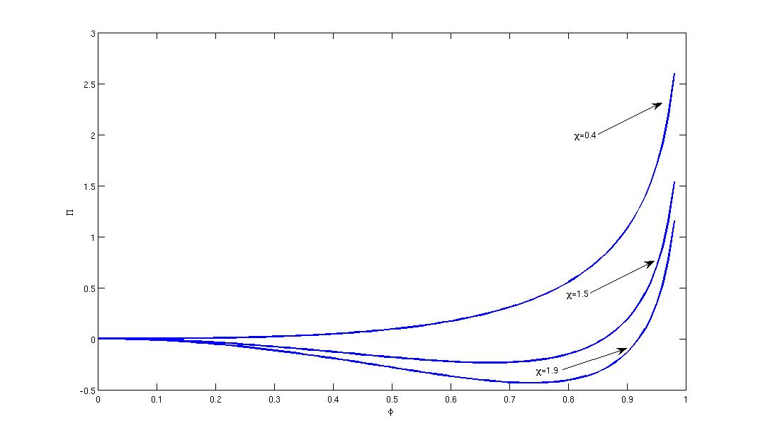
Fig. 1: These are plots of the osmotic pressure of the gel with respect to the polymer volume fraction $\phi$. We point out the change of monotonicity of the graphs with respect to $\chi$. Such phenomenon corresponds to phase separation in the gel.

We let $\mathcal{T}_{i}^{r}$ and $\mathcal{T}_{i}^{v},i=1,2$ denote the reversible and the viscous components of the gel stress, respectively. So, the total stress of the $i$-component is $\mathcal{T}_{i}=\mathcal{T}^{r}_{i}+\mathcal{T}^{v}_{i},\,i=1,2$, with $\mathcal{T}^{r}_{2}=0$. Moreover, we assume that the dissipative stress of each component is Newtonian,

$$\mathcal{T}_{i}^{v}= \eta_{i}\mathbf{D}(\mathbf{v}_{i})+\mu_{i}(\nabla\cdot\mathbf{v}_{i})I,\,\,\mathcal{T}_{b}=\frac{\eta_{2}}{2}D(\mathbf{v}_{b})\,\,$$

$$\quad\mathbf{D}(\mathbf{v}):=\frac{1}{2}(\nabla\mathbf{v}+\nabla\mathbf{v}^{T}),$$

$i=1,2$; $\eta_{i}>0$ and $\mu_{i}>0$ denote the shear and bulk viscosity coefficients, respectively, of the components. The total stress $\mathcal{T}$ of the gel is

$$\mathcal{T}=\mathcal{T}_{1}+\mathcal{T}_{2}.$$ (26)

From now on, we will treat (7) as a constraint, and let $p$ denote the corresponding Lagrange multiplier. Letting $\epsilon({\mathbf{x}},t)$ denote the internal energy density of the gel and $\zeta({\mathbf{x}},t)=\frac{1}{\theta}(\epsilon({\mathbf{x}},t)-\psi({\mathbf{x}},t))$ the entropy density, the Clausius-Duhem inequality states that $\dot{\zeta}\geq 0$ holds, for all admissible processes of the gel. This allows us to establish the following proposition, which proof is presented in [8].

Proposition 1.

Suppose that the Clausius-Duhem inequality holds for all admissible processes, and let $\{\mathbf{v}_{i},\phi_{i},p\}$ smooth solutions of equations (2), (4), (6), (7), (11), (12) and (2.3). Suppose that the boundary conditions (8)-(12) are satisfied. Then the following relations hold:

$$\mathcal{T}^{r}_{1}=\hat{\sigma}-\pi I,\,\,\hat{\sigma}=\phi_{1}\frac{\partial W}{\partial F}F^{T}$$ (27)

$$\pi=\phi_{1}(\frac{\partial G}{\partial\phi_{1}}-\frac{\partial G}{\partial\phi_{2}})-G.$$ (28)

Moreover, the dissipation inequality

$$\frac{d\mathcal{F}}{dt}= -\int_{\Omega_{t}}\bigg{(}\eta_{i}{\big{|}\!\big{|}}\mathbf{D}(\mathbf{v}_{i}){\big{|}\!\big{|}}^{2}+\mu_{i}(\nabla\cdot\mathbf{v}_{i})^{2}+\eta{\big{|}\!\big{|}}\mathbf{v}_{1}-\mathbf{v}_{2}{\big{|}\!\big{|}}^{2}\bigg{)}\,d{\mathbf{y}}-\int_{\partial\Omega_{t}}(\eta_{\perp}w^{2}+\eta_{\|}|\mathbf{q}|^{2})\,dS,$$

holds, where ${\mathbf{n}}$ denotes the unit outward normal to the boundary.

As a result of the required material frame-indifference, there exists a function $\hat{W}$ defined on the space of symmetric, positive definite tensors, such that $W(F)=\hat{W}(C),$ where $C=F^{T}F$. We let $\mathcal{P}=2\phi_{I}\frac{\partial\hat{W}(C)}{\partial C}$ denote the second Piola-Kirchhoff stress tensor. We further assume that the polymer is an isotropic elastic material, so there is a scalar function $w$ of the principal invariants $\mathcal{I}=\{I_{1},I_{2},I_{3}\}$ of $C$, such that $\hat{W}(C)=w(\mathcal{I})$. In this case, the following representation holds ([27], page 279):

$$\frac{\partial\hat{W}}{\partial C}=\alpha_{1}(\mathcal{I})I+\alpha_{2}(\mathcal{I})C+\alpha_{0}(\mathcal{I})C^{-1},$$ (30)

$$\alpha_{0}=I_{3}\frac{\partial w}{\partial I_{3}},\quad\alpha_{1}=\frac{\partial w}{\partial I_{1}}+I_{1}\frac{\partial w}{\partial I_{2}},\quad\alpha_{2}=-\frac{\partial w}{\partial I_{2}}.$$ (31)

The Cauchy stress tensor $\hat{\sigma}=\frac{1}{\det F}F\mathcal{P}(C)F^{T}$ in (27) has the form,

$$\hat{\sigma}=\phi_{\textrm{\tiny I}}\big{(}\beta_{0}({\mathcal{I}})I+\beta_{1}({\mathcal{I}})B+\beta_{2}({\mathcal{I}})B^{-1}\big{)},$$ (32)

$$\beta_{0}=\frac{2}{\sqrt{I}_{3}}(I_{2}\frac{\partial w}{\partial I_{2}}+I_{3}\frac{\partial w}{\partial I_{3}}),\,\,\beta_{1}=\frac{2}{\sqrt{I}_{3}}\frac{\partial w}{\partial I_{1}},\,\,\beta_{2}=-2\sqrt{I_{3}}\frac{\partial w}{\partial I_{2}}.$$ (33)

Example 2.3.1.

Let us consider a Hadamard material ([11], [26]),

$$w(I_{1},I_{2},I_{3})=\frac{{\mu_{\textrm{\tiny E}}}}{2}\big{(}\frac{a_{1}}{s}I_{1}^{s}+\frac{\alpha}{r}I_{3}^{-r}+\frac{a_{3}}{q}I_{3}^{q}\big{)},\quad\mu_{E}=K\theta\mu_{x},$$ (34)

$$\hat{\sigma}=\frac{\phi_{I}{\mu_{\textrm{\tiny E}}}}{\sqrt{I}_{3}}\big{(}\nu B-\kappa I\big{)},$$ (35)

$$\nu=\nu(\mathcal{I})=a_{1}I_{1}^{s-1},\quad\kappa=\kappa(\mathcal{I})=\frac{1}{{\mu_{\textrm{\tiny E}}}\phi_{\textrm{\tiny I}}}{\pi\sqrt{I_{3}}}+\alpha I_{3}^{-r}-a_{3}I_{3}^{q},$$ (36)

$$\beta_{1}=\frac{\phi_{I}{\mu_{\textrm{\tiny E}}}}{\sqrt{I}_{3}}\nu,\,\,\beta_{2}=0,\,\,\beta_{0}=-\frac{\phi_{I}{\mu_{\textrm{\tiny E}}}}{\sqrt{I}_{3}}\kappa,$$ (37)

where $\alpha>0$, $a_{1}>0,a_{3}>0,$ $q,s,r\geq 1$ are constant. The parameter $\mu_{x}$ represents the crosslink density of the network.

Stress free bulk equilibrium states $(\phi_{0},F_{0},p_{0})$ are constant fields satisfying (6), and

$$\mathcal{T}_{1}^{r}(F_{0},\phi_{0})-\phi_{0}p_{0}I=0,\quad-(1-\phi_{0})p_{0}=0,$$ (38)

with $\mathcal{T}_{1}^{r}$ as in (27). It is easy to check that the former reduce to

$$\beta_{1}f^{2}+\beta_{2}f^{-2}=\phi_{I}^{-1}{\pi(\phi)}-\beta_{0},\,\,{\textrm{where}}$$ (39)

$$B=f^{2}I,\,\,\phi=\phi_{I}f^{-\frac{3}{2}},\,\,f>0.$$ (40)

For the energy in (34), equations (38) become $\nu B=\kappa I,$ with $\nu$ and $\kappa$ as in (36). Equivalently,

$$\frac{\pi(\phi)}{{\mu_{\textrm{\tiny E}}}\phi}+\alpha(\frac{\phi}{\phi_{\textrm{\tiny I}}})^{2r}-a_{3}(\frac{\phi_{\textrm{\tiny I}}}{\phi})^{2q}=a_{1}3^{s-1}(\frac{\phi_{\textrm{\tiny I}}}{\phi})^{\frac{2}{3}s},$$ (41)

with $\pi(\phi)$ as in (23) and (28). We summarize the previous statements in the following:

Proposition 2.

Suppose that the gel is isotropic. Then the stress free bulk states are uniform dilations or compressions satisfying equation (39) and (40). In the case that the energy is given by (34), there is a unique equilibrium state provided the material parameters satisfy

$$\frac{\alpha}{\phi_{\textrm{\tiny I}}}>a_{1}3^{s-1}\phi_{\textrm{\tiny I}}^{\frac{2s}{3}}+a_{3}\phi_{\textrm{\tiny I}}^{2q}+\frac{1}{{\mu_{\textrm{\tiny E}}}}(c+b-a).$$ (42)

Moreover, $\kappa(\phi_{0})>0$, and $\phi_{0}>\phi^{*}>0$, where $\phi^{*}$ satisfies $\kappa(\phi^{*})=0$.

Remarks.  We point out that the assumptions on the coefficients of $w$ and $G$ are sufficient to guarantee the existence of a global minimizer of the total energy under appropriately prescribed boundary conditions [2], including those of displacement-traction type. Inequality (42) gives insights on material parameter ranges that guarantee existence of unique stress free equilibrium states.

1. Phase separation may occur for material parameters such that $\kappa(\phi)$ is non-monotonic. A necessary condition for the latter to occur is that $c>0$ in (24) be sufficiently large, and therefore it corresponds to the case that $\pi(\phi)$ has negative intervals; in device applications, usually $c=.5$. This is illustrated in Figure 2.1.

2. Holding $c$ fixed, small values of $\alpha>0$ or ${\mu_{\textrm{\tiny E}}}>0$ may also lead to phase separation. The latter correspond to prescribing small shear and bulk moduli. Moreover, the equilibrium value $0<\phi_{0}<1$ also increases with respect to ${\mu_{\textrm{\tiny E}}}$

We now let $\phi_{0},F_{0}$ denote a solution of the boundary value problem

$$\nabla\cdot\mathcal{T}_{1}^{r}(F,\phi)=0,\quad\phi\det F=\phi_{\textrm{\tiny I}},\,\,\,p=\textrm{constant},$$ (43)

subject to mixed displacement-traction boundary conditions.

3 Linear problems

We now linearize the governing system (4), (5), (6) and (7) about a particular time independent solution $(\phi_{0},F_{0},p_{0}=0,\mathbf{v}_{1}=\mathbf{0}=\mathbf{v}_{2})$. Relevant special cases include stress-free dilation or compression states $F_{0}=f_{0}I$, and also non-stress free equilibria. The tilde notation represents perturbations from the equilibrium state, which is labeled with $0$-super (or sub) indices. Let $\tilde{F}:={\nabla_{\tiny{{\mathbf{x}}}}}\tilde{\mathbf{u}}$, and

$$\phi=\phi_{0}+\tilde{\phi},\,\,F=F_{0}+\tilde{F},\,\,p=\tilde{p},\,\,\mathbf{v}_{1}=\tilde{\mathbf{v}},\,\,\mathbf{v}_{2}=\tilde{\mathbf{w}}.$$ (44)

The gel domain now corresponds to the reference configuration, $\Omega$, of the polymer. First, we calculate the linear swelling ratio and polymer volume fraction:

$$\det F=\phi_{0}\det F_{0}(1+\gamma({\nabla_{\tiny{{\mathbf{x}}}}}\tilde{\mathbf{u}}))+o(|{\nabla_{\tiny{{\mathbf{x}}}}}\tilde{\mathbf{u}}|^{2}),$$ (45)

$$\phi=\phi_{0}(1-\gamma({\nabla_{\tiny{{\mathbf{x}}}}}\tilde{\mathbf{u}}))+o(|{\nabla_{\tiny{{\mathbf{x}}}}}\tilde{\mathbf{u}}|^{2}),$$ (46)

where $\gamma({\nabla_{\tiny{{\mathbf{x}}}}}\tilde{\mathbf{u}})={\textrm{tr\,}}(F_{0}^{-1}{\nabla_{\tiny{{\mathbf{x}}}}}\tilde{\mathbf{u}})$. Letting $C_{0}=F^{T}_{0}F_{0}$, we denote

$$\mathfrak{C}_{ijkl}= 2\frac{\partial^{2}\hat{W}}{\partial C_{ij}\partial C_{kl}}(C_{0})=\frac{\partial\mathcal{P}_{0}}{\partial C}(C_{0}),$$ (47)

$$\pi^{0}= \pi(\phi_{0},1-\phi_{0}),\quad\pi^{0}_{j}=\frac{\partial\pi}{\partial\phi_{j}}(\phi_{0},1-\phi_{0}),\,\,\,j=1,2.$$ (48)

The fourth order tensor with components $\mathfrak{C}_{ijkl}$ corresponds to the elasticity matrix, with the symmetry properties

$$\mathfrak{C}_{ijkl}=\mathfrak{C}_{klij}=\mathfrak{C}_{jikl}=\mathfrak{C}_{ijlk}.$$ (49)

The quantities (45)-(48) yield the linearized expressions of the stress tensors. These equations are exact up to terms of order $o(|{\nabla_{\tiny{{\mathbf{x}}}}}\tilde{\mathbf{u}}|^{2})$):

$$\hat{\sigma}= \hat{\sigma}_{0}+\phi_{0}\{-F_{0}\mathcal{P}_{0}F_{0}^{T}\gamma({\nabla_{\tiny{{\mathbf{x}}}}}\tilde{\mathbf{u}})+F_{0}\mathfrak{C}(F_{0}^{T}{\nabla_{\tiny{{\mathbf{x}}}}}\tilde{\mathbf{u}}+{\nabla_{\tiny{{\mathbf{x}}}}}\tilde{\mathbf{u}}^{T}F_{0})F^{T}_{0}$$ (50)

$$+\big{(}F_{0}\mathcal{P}_{0}{\nabla_{\tiny{{\mathbf{x}}}}}\tilde{\mathbf{u}}^{T}+{\nabla_{\tiny{{\mathbf{x}}}}}\tilde{\mathbf{u}}\mathcal{P}_{0}F_{0}^{T}\big{)}\},$$

$$\pi= \pi^{0}-\phi_{0}(\pi_{1}^{0}-\pi_{2}^{0})\,\gamma({\nabla_{\tiny{{\mathbf{x}}}}}\tilde{\mathbf{u}}),$$

$$\mathcal{T}= \mathcal{T}_{1}^{r}=\mathcal{T}_{1}^{r,0}+(\phi_{0}\big{(}\pi_{1}^{0}-\pi_{2}^{0})I-\hat{\sigma}(F_{0},\phi_{0})\big{)}\gamma({\nabla_{\tiny{{\mathbf{x}}}}}\tilde{\mathbf{u}})$$ (51)

$$+\phi_{0}\{F_{0}\mathfrak{C}(F_{0}^{T}{\nabla_{\tiny{{\mathbf{x}}}}}\tilde{\mathbf{u}}+{\nabla_{\tiny{{\mathbf{x}}}}}\tilde{\mathbf{u}}^{T}F_{0})F^{T}_{0}+\big{(}F_{0}\mathcal{P}_{0}{\nabla_{\tiny{{\mathbf{x}}}}}\tilde{\mathbf{u}}^{T}+{\nabla_{\tiny{{\mathbf{x}}}}}\tilde{\mathbf{u}}\mathcal{P}_{0}F_{0}^{T}\big{)}\}$$

The linearized system of equations is

$$\nabla\cdot(\phi_{0}\tilde{\mathbf{v}}+(1-\phi_{0})\tilde{\mathbf{w}})=0,$$ (52)

$$\nabla\cdot\mathcal{T}_{1}-\beta(\tilde{\mathbf{v}}-\tilde{\mathbf{w}})-\phi_{0}\nabla p=\mathbf{0},$$ (53)

$$\nabla\cdot\mathcal{T}_{2}+\beta(\tilde{\mathbf{v}}-\tilde{\mathbf{w}})-(1-\phi_{0})\nabla p=\mathbf{0},$$ (54)

$$\mathcal{T}_{1}({\nabla_{\tiny{{\mathbf{x}}}}}\tilde{\mathbf{u}},\nabla\tilde{\mathbf{v}})=\mathcal{T}_{1}^{r}({\nabla_{\tiny{{\mathbf{x}}}}}\tilde{\mathbf{u}})+\eta_{1}\mathbf{D}(\tilde{\mathbf{v}})+\mu_{1}(\nabla\cdot\tilde{\mathbf{v}})I,$$ (55)

$$\mathcal{T}_{2}({\nabla_{\tiny{{\mathbf{x}}}}}\tilde{\mathbf{u}},\nabla\tilde{\mathbf{w}})=\eta_{2}\mathbf{D}(\tilde{\mathbf{w}})+\mu_{2}(\nabla\cdot\tilde{\mathbf{w}})I.$$ (56)

$$\tilde{\mathbf{u}}_{t}=\tilde{\mathbf{v}},$$ (57)

together with (46). We point out that the last equation follows from the linearization of (5), neglecting uniform translations:

$${\nabla_{\tiny{{\mathbf{x}}}}}\dot{\mathbf{u}}=(\nabla\mathbf{v}_{1})F_{0}.$$ (58)

3.1 Stability of Equilibrium Solutions

The conditions that guarantee the stability of the equilibrium states turn out to be also necessary conditions for the solvability of the time-dependent, quasi-static problem, that we study in later sections. In order to established such conditions, we first outline the properties of the second order tensor $\mathcal{P}$ and that of the fourth order one $\mathfrak{C}$. Unlike the case of linearizing about a stress free state, here we need to include $\mathcal{T}_{r}^{0}$ in the analysis of stability.

Notation.  With the understanding that the quantities that we study are evaluated at $F_{0},C_{0}=F^{T}_{0}F_{0}$, in this section, we suppress the $0$-notation in the equilibrium solution, and the $\it tilde$ symbol in the perturbation terms, unless explicitly needed. The fourth order elasticity tensor

$$\mathfrak{C}_{ijpq}(C) ={\scriptsize\mathcal{A}}_{1}\delta_{pq}\delta_{ij}+{\scriptsize\mathcal{A}}_{2}({\textrm{tr\,}}C\delta_{pq}-C_{pq})C_{ij}+{\scriptsize\mathcal{A}}_{3}(\det C)C_{pq}^{-T}C_{ij}^{-1}$$ (59)

$$+\alpha_{2}\delta_{ip}\delta_{jq}-\alpha_{0}C^{-1}_{ip}C^{-1}_{qj},\,\,{\scriptsize{\mathcal{A}}}_{m}=\sum_{n=0}^{2}\frac{\partial\alpha_{n}}{\partial I_{m}},\,\,\,m=1,2,3.$$

In the case that $C$ corresponds to a pure expansion or compression, $C=f^{2}I$, $f>0$, we obtain the following representations.

$$\mathfrak{C}_{ijpq}= \lambda(f)\delta_{ij}\delta_{pq}+2\mu(f)\delta_{ip}\delta_{jq},\quad\textrm{with}$$ (60)

$$\lambda= \sum_{n=0}^{2}\big{(}\frac{\partial\alpha_{n}}{\partial I_{1}}+\frac{\partial\alpha_{n}}{\partial I_{2}}f^{4}+\frac{\partial\alpha_{n}}{\partial I_{3}}f^{2}\big{)},\quad\mu=\alpha_{2}-\alpha_{0}f^{-4}.$$ (61)

Moreover, the total linearized stress tensor (51) becomes

$$\mathcal{T}^{r}=2\tilde{\mu}\mathbf{D}({\mathbf{u}})+\tilde{\lambda}{\textrm{tr\,}}{\mathbf{D}({\mathbf{u}})}I,\quad{\textrm{with}}$$ (62)

$$\tilde{\mu}=\phi_{\textrm{\tiny I}}\big{(}2\mu+f_{0}^{-2}(\alpha_{1}+\alpha_{2}f_{0}^{2}+\alpha_{0}f_{0}^{-2}\big{)},$$ (63)

$$\tilde{\lambda}=\phi_{0}(\pi_{1}^{0}-\pi_{2}^{0})-\pi^{0}+2\phi_{\textrm{\tiny I}}\lambda.$$ (64)

Likewise, the analog of the fourth order tensor (59) that combines the elastic and Flory-Huggins effects is

$${\tilde{\mathfrak{C}}}_{ijpq}=\tilde{\lambda}(f)\delta_{ij}\delta_{pq}+2\tilde{\mu}(f)\delta_{ip}\delta_{jq}.$$ (65)

Proposition 3.

Let $f>0$. Suppose that

$$\tilde{\mu}(f)>0,\quad 3\tilde{\lambda}(f)+2\tilde{\mu}(f)>0,$$ (66)

hold. Then $\tilde{\mathfrak{C}}$ in (65) is coercive, that is, there exists a constant $\mu_{0}>0$ such that

$${\tilde{\mathfrak{C}}}_{ikls}A_{ik}A_{ls}\geq\mu_{0}|A|^{2}$$ (67)

holds, for all $A\in M^{3\times 3}$.

For the Hadamard energy in (34), with $\kappa$ and $\nu$ as in (36), we have

$$\tilde{\mu}=\phi_{\textrm{\tiny I}}(f^{-2}\kappa+\nu)f^{-2},\quad\tilde{\lambda}=\phi(\pi_{1}^{0}-\pi_{2}^{0})-\pi^{0}+2\phi_{\textrm{\tiny I}}\lambda.$$ (68)

3.1.1 General equilibrium state

We assume that $(F_{0},\phi_{0})$ is a solution of (43), and let $\mathcal{T}^{r}$ be as in (51), with the elasticity tensor $\mathfrak{C}$ given by (59). We say that an equilibrium solution is locally stable if

$$\mathcal{T}^{r}(F_{0},\phi_{0})\cdot\nabla\mathbf{v}\geq 0,$$ (69)

for all sufficiently smooth fields ${\mathbf{u}},\mathbf{v}$ satisfying (58). We now derive sufficient conditions for the stability of equilibrium solutions. Let us introduce the following notation.

$$C_{2}:=\frac{\partial^{2}w}{\partial I_{1}^{2}}+\frac{\partial^{2}w}{\partial I_{1}\partial I_{3}}I_{3},\quad C_{3}=I_{3}^{2}\frac{\partial^{2}w}{\partial I_{3}^{2}}+\frac{\phi_{1}}{2}\pi_{1,2}.$$ (70)

Proposition 4.

Suppose that $w=w(I_{1},I_{3})$ and that relations (30)-(33) and (58) hold. Let $0<\phi_{0}({\mathbf{x}})<1$ and $F_{0}({\mathbf{x}})\in\mathcal{M}^{n\times n}_{+},\,{\mathbf{x}}\in\Omega$, be an equilibrium solution. Then

$$\mathcal{T}^{r}\cdot\nabla\mathbf{v}=\mathcal{T}^{r}_{0}\cdot\nabla\mathbf{v}+\phi_{\textrm{\tiny I}}\frac{\partial}{\partial t}\mathcal{H},$$ (71)

where

$$\mathcal{H}:=\mathfrak{C}({\nabla_{\tiny{{\mathbf{x}}}}}{\mathbf{u}}^{T}F_{0})\cdot({\nabla_{\tiny{{\mathbf{x}}}}}{\mathbf{u}}^{T}F_{0})^{T}+\mathfrak{D}({\nabla_{\tiny{{\mathbf{x}}}}}{\mathbf{u}};F_{0})+\frac{1}{2}\pi_{1,2}^{0}\,{\textrm{tr\,}}^{2}(F_{0}^{-1}{\nabla_{\tiny{{\mathbf{x}}}}}{\mathbf{u}}),$$ (72)

$$\mathfrak{C}({\nabla_{\tiny{{\mathbf{x}}}}}{\mathbf{u}}^{T}F_{0})\cdot({\nabla_{\tiny{{\mathbf{x}}}}}{\mathbf{u}}^{T}F_{0})=C_{2}\,{\textrm{tr\,}}^{2}({\nabla_{\tiny{{\mathbf{x}}}}}{\mathbf{u}}^{T}F_{0})+I_{3}^{2}\frac{\partial^{2}w}{\partial I_{3}^{2}}\,{\textrm{tr\,}}^{2}(F^{-1}_{0}{\nabla_{\tiny{{\mathbf{x}}}}}{\mathbf{u}})-I_{3}\frac{\partial w}{\partial I_{3}}|({\nabla_{\tiny{{\mathbf{x}}}}}{\mathbf{u}})F^{-1}_{0}|^{2},$$ (73)

$$\mathfrak{D}({\nabla_{\tiny{{\mathbf{x}}}}}{\mathbf{u}};F_{0}):=\frac{\alpha_{0}}{2}{\textrm{tr\,}}\big{(}(F^{-T}_{0}{\nabla_{\tiny{{\mathbf{x}}}}}{\mathbf{u}}^{T})^{2}+{\nabla_{\tiny{{\mathbf{x}}}}}{\mathbf{u}}\,C^{-1}_{0}{\nabla_{\tiny{{\mathbf{x}}}}}{\mathbf{u}}^{T}\big{)}+\alpha_{1}\big{(}F_{0}{\nabla_{\tiny{{\mathbf{x}}}}}{\mathbf{u}}^{T}\cdot{\nabla_{\tiny{{\mathbf{x}}}}}{\mathbf{u}}\,F^{-1}_{0}+|{\nabla_{\tiny{{\mathbf{x}}}}}{\mathbf{u}}|^{2}),$$ (74)

$$\pi^{0}_{1,2}(\phi_{1}):=\pi_{1}^{0}-\pi_{2}^{0}=a-b-2c\phi_{1}+\frac{b}{1-\phi_{1}}.$$ (75)

Proof.

Starting with

$$\mathcal{T}^{r}\cdot\nabla\mathbf{v}= \bigg{(}\mathcal{T}_{r}^{0}+\phi_{\textrm{\tiny I}}\{F_{0}\mathfrak{C}(F_{0}^{T}{\nabla_{\tiny{{\mathbf{x}}}}}\tilde{\mathbf{u}}+{\nabla_{\tiny{{\mathbf{x}}}}}\tilde{\mathbf{u}}^{T}F_{0})F^{T}_{0}$$

$$+ \big{(}F_{0}\mathcal{P}_{0}{\nabla_{\tiny{{\mathbf{x}}}}}\tilde{\mathbf{u}}^{T}+{\nabla_{\tiny{{\mathbf{x}}}}}\tilde{\mathbf{u}}\mathcal{P}_{0}F_{0}^{T}\big{)}\}+\phi_{\textrm{\tiny I}}(\pi_{1}^{0}-\pi_{2}^{0})I)\gamma(F_{0}^{-1}{\nabla_{\tiny{{\mathbf{x}}}}}{\mathbf{u}})\bigg{)}\cdot\nabla\mathbf{v},$$ (76)

straightforward calculations that apply (58) give

$$\frac{\partial}{\partial t}\big{(}\mathfrak{C}({\nabla_{\tiny{{\mathbf{x}}}}}{\mathbf{u}}^{T}F_{0})\cdot({\nabla_{\tiny{{\mathbf{x}}}}}{\mathbf{u}}^{T}F_{0})\big{)}=\mathfrak{C}({\nabla_{\tiny{{\mathbf{x}}}}}{\mathbf{u}}^{T}F_{0}+F_{0}^{T}{\nabla_{\tiny{{\mathbf{x}}}}}{\mathbf{u}})\cdot({\nabla_{\tiny{{\mathbf{x}}}}}\dot{\mathbf{u}}^{T}F_{0}),$$ (77)

$$\frac{\partial\mathfrak{D}}{\partial t}=(F_{0}\mathcal{P}_{0}{\nabla_{\tiny{{\mathbf{x}}}}}{\mathbf{u}}^{T}+{\nabla_{\tiny{{\mathbf{x}}}}}{\mathbf{u}}\mathcal{P}_{0}F^{T}_{0})\cdot\nabla\mathbf{v},$$ (78)

$$\frac{\partial}{\partial t}(\frac{\phi_{\textrm{\tiny I}}}{2}\pi^{0}_{1,2}\,{\textrm{tr\,}}^{2}(F^{-1}_{0}{\nabla_{\tiny{{\mathbf{x}}}}}{\mathbf{u}}))=\phi_{\textrm{\tiny I}}\pi^{0}_{1,2}{\textrm{tr\,}}(F^{-1}_{0}{\nabla_{\tiny{{\mathbf{x}}}}}{\mathbf{u}})I\cdot({\nabla_{\tiny{{\mathbf{x}}}}}\dot{\mathbf{u}}F^{-1}_{0}),$$ (79)

where $\mathcal{P}$ is given in (30). ∎

Next, we establish coercivity of the operator $\mathcal{H}$ in (72). For this, let us write

$$\mathcal{H}:=\mathcal{H}_{1}+\mathcal{H}_{2},$$ (80)

$$\mathcal{H}_{1}:=C_{2}{\textrm{tr\,}}^{2}(\nabla{\mathbf{u}}^{T}F_{0})+C_{3}{\textrm{tr\,}}^{2}(F^{-1}_{0}\nabla{\mathbf{u}})-\alpha_{0}|\nabla{\mathbf{u}}F^{-1}_{0}|^{2}+\frac{\alpha_{0}}{2}{\textrm{tr\,}}(\nabla{\mathbf{u}}C_{0}^{-1}\nabla{\mathbf{u}}^{T}),$$ (81)

$$\mathcal{H}_{2}:=\frac{\alpha_{0}}{2}{\textrm{tr\,}}(F^{-T}_{0}\nabla{\mathbf{u}}^{T})^{2}+\alpha_{1}(F_{0}\nabla{\mathbf{u}}^{T}\cdot\nabla{\mathbf{u}}F^{-1}_{0}+|\nabla{\mathbf{u}}|^{2}).$$ (82)

Lemma 5.

Let $a,b$, $c$ be as in (23) and $0<\chi\leq 0.5$. Then $\pi^{0}_{1,2}>0$ is monotonically increasing. Moreover if for each $I_{1}>0$, $w(I_{1},I_{3})$ is convex with respect to $I_{3}$, then $C_{3}>0$.

This condition on $\chi$ is satisfied in gels used in device applications. The monotonicity of $\pi^{0}_{1,2}$ for this range of $\chi$ is illustrated in Figure 2.1.

Proposition 6.

Suppose that the assumptions of Lemma 3.3 hold. Assume that $\alpha_{0}<0$ and that $C_{2}>0$. Then

$$\mathcal{H}_{1}\geq|\alpha_{0}||\nabla{\mathbf{u}}F^{-1}_{0}|^{2}+C_{2}{\textrm{tr\,}}^{2}(\nabla{\mathbf{u}}^{T}F_{0})+C_{3}{\textrm{tr\,}}^{2}(F^{-1}_{0}\nabla{\mathbf{u}}).$$ (83)

Next, we study the coercivity of $\mathcal{H}$. Let us consider the polar decomposition $F=RV$, where $R$ denotes the rotation tensor, and $V=\sqrt{C}$. Let $\lambda_{i},\,i=1,2,3$ denote the eigenvalues of $C$. Let us denote

$$N:= ({\nabla_{\tiny{{\mathbf{x}}}}}{\mathbf{u}}^{T})R,$$ (84)

$$\Gamma_{ij}:= h_{ij}N_{ij}N_{ji},\quad h_{ij}:=\frac{\alpha_{0}+\alpha_{1}(\lambda_{i}+\lambda_{j})}{\sqrt{\lambda_{i}\lambda_{j}}},\quad i\neq j.$$ (85)

We now calculate $\mathcal{H}_{2}$ using its representation in terms of the eigenvector basis of $C$,

$$\mathcal{H}_{2}= \frac{\alpha_{0}}{2}\sum_{I}\lambda_{i}^{-1}N_{ii}^{2}+\frac{\alpha_{0}}{2}\sum_{i\neq j}\Gamma_{ij}+2\alpha_{1}\sum_{i}N_{ii}^{2}+\alpha_{1}\sum_{i\neq j}N_{ij}^{2}$$ (86)

We combine the first term of the right hand side of $\mathcal{H}_{2}$ with the last one on the right hand side of $\mathcal{H}_{1}$ (81) (which can also be written in terms of $N_{ij}$). We also combine the mixed products in $\Gamma_{ij}$ with the last term in $\mathcal{H}_{2}$, upon application of the Cauchy-Schwartz inequality. We now state

Theorem 7.

Let $(F_{0},\phi_{0})$ be an equilibrium solution. Suppose that the assumptions of Proposition 3.4 hold. Furthermore, we assume that $C_{2}>0$ in (70) and

$$\alpha_{1}>\frac{1}{2}\max_{i\neq j}|h_{ij}|.$$ (87)

Then

$$\mathcal{H}\geq\frac{|\alpha_{0}|}{2}|\nabla{\mathbf{u}}F^{-1}_{0}|^{2}+C_{2}{\textrm{tr\,}}^{2}(\nabla{\mathbf{u}}^{T}F_{0})+C_{3}{\textrm{tr\,}}^{2}(F^{-1}_{0}\nabla{\mathbf{u}}).$$ (88)

Remarks. 

1.  Inequalities (66) and (67) (for a spherical equilibrium state), and the positivity of $C_{2}$ and $C_{3}$ in (70) (for an arbitrary equilibrium state) correspond to the strong ellipticity of the linear operator. Strong ellipticity guarantees regularity of the weak solutions of the linear problem. In the case that $F_{0}=f_{0}I$, the assumptions of Theorem 3.5 imply inequalities (66) to hold.

2.  The need to separately account for stretch and rotation in the proof of Theorem 3.5 is a signature feature of linear elasticity, when the equilibrium state is not stress free. In particular, the theorem applies to the linearization about the reference configuration, even if the residual stress is nonzero. In this case, inequality (87) is identically satisfied.

3.2 Initial, boundary-value problems

We formulate the governing equations in terms of homogeneous boundary conditions on the displacement field, which also satisfies the only initial condition to be specified in the problem,

$$\mathbf{\tilde{u}}|_{t=0}=\mathbf{\tilde{u}}_{0},\quad\mathbf{\tilde{u}}_{0}|_{\Gamma_{0}}=\tilde{\mathbf{U}}|_{t=0}.$$ (89)

The latter is a compatibility condition with the boundary data at $t=0$. Assume that $\Gamma_{0}$ is of class $C^{m}$, for some given integer $m\geq 1$, and $\tilde{\mathbf{U}}\in H^{m-1/2}(\Gamma_{0})$. We let ${\mathbf{U}}$ denote the extension of $\tilde{\mathbf{U}}$ to $\Omega$, so that $||{\mathbf{U}}||_{H^{m}({\Omega})}\leq C||\tilde{\mathbf{U}}||_{H^{m-1/2}(\Gamma_{0})}$ [24, p. 68]. From now on, we will set $m=2$. We also assume $P_{0}\in H^{1/2}({\partial\Omega})$ and ${\partial\Omega}\in C^{1}$. Then $\exists P\in H^{1}({\Omega})$ such that $P|_{{\partial\Omega}}=P_{0}$ and $||P||_{H^{1}({\Omega})}\leq C||P_{0}||_{H^{1/2}({\partial\Omega})}$.

Let,

$$\bar{\mathbf{u}}=\mathbf{\tilde{u}}-{\mathbf{U}},\quad\bar{\mathbf{u}}_{0}=\mathbf{\tilde{u}}_{0}-\mathbf{U}_{t=0},\quad\bar{\mathbf{v}}_{2}=\tilde{\mathbf{v}}_{2}-\mathbf{V}\quad\textrm{and}\quad\bar{p}=\tilde{p}-P,\quad\bar{\mathbf{u}}_{t}=\mathbf{v}_{1},$$ (90)

where $\mathbf{V}$ and $P$ are defined as follows:

$$\mathbf{V}=\mathbf{U}_{t},\,\,P=0\,\,$$ (91)

$$\mathbf{V}=0,\,\,P\,\textrm{ is the extension of}\,P_{0},$$ (92)

for impermeable and fully permeable boundary, respectively. The governing system reduces now to

$$\nabla\cdot({\phi_{0}}\bar{\mathbf{u}}_{t}+(1-{\phi_{0}})\bar{\mathbf{v}}_{2})=h,$$ (93)

$$\nabla\cdot\mathcal{T}_{1}({\nabla_{\tiny{{\mathbf{x}}}}}\bar{\mathbf{u}},\nabla\bar{\mathbf{v}}_{1})-\phi_{0}\nabla\bar{p}-\beta(\bar{\mathbf{u}}_{t}-\bar{\mathbf{v}}_{2})=\mathbf{f}_{1},$$ (94)

$$\nabla\cdot\mathcal{T}_{2}({\nabla_{\tiny{{\mathbf{x}}}}}\bar{\mathbf{u}},\nabla\bar{\mathbf{v}}_{2})-(1-\phi_{0})\nabla\bar{p}+\beta(\bar{\mathbf{u}}_{t}-\bar{\mathbf{v}}_{2})=\mathbf{f}_{2},$$ (95)

with $\mathcal{T}_{1}$ and $\mathcal{T}_{2}$ as in (55) and (56), respectively, and

$$h=-\nabla\cdot({\phi_{0}}{\mathbf{U}}_{t}+(1-{\phi_{0}}){\mathbf{V}}),\,\,\kappa=\frac{1}{\beta}(1-{\phi_{0}})^{2},$$ (96)

$$\mathbf{f}_{1}=-\nabla\cdot\mathcal{T}_{1}(\mathbf{D}({\mathbf{U}}),\mathbf{D}({\mathbf{U}}_{t}))+\phi_{0}\nabla P+\beta({\mathbf{U}}_{t}-{\mathbf{V}})$$ (97)

$$\mathbf{f}_{2}=-\nabla\cdot\mathcal{T}_{2}(\mathbf{D}({\mathbf{V}}))+(1-\phi_{0})\nabla P-\beta({\mathbf{U}}_{t}-{\mathbf{V}})$$ (98)

$$\mathbf{G}=(P-P_{0}){\mathbf{n}}-\mathcal{T}(\mathbf{D}(\mathbf{U}),\mathbf{D}(\mathbf{U}_{t}),\mathbf{D}({\mathbf{V}})){\mathbf{n}},\,\,\textrm{on}\,\partial\Omega,$$ (99)

$$H=h+\nabla\cdot(\frac{1-\phi_{0}}{\beta})\mathbf{f}_{2}:=-\nabla\cdot\mathbf{\mathcal{H}},$$ (100)

Notation.  We suppress the superimposed bar on the unknown fields, and write $({\mathbf{u}},\mathbf{v}_{2},p)$.

Without loss of generality, in sections 4 and 5, we consider linearization of the original system about uniform expansion or compression, $F_{0}=f_{0}I$. With the help of the energy law developed in section 6, these results can be easily extended to the case of a general equilibrium state.

4 Inviscid solvent

We prove existence and uniqueness of weak solution in the case that the fluid component is inviscid. Setting $\eta_{2}=0$ and $\mu_{2}=0$ in (56) and solving it explicitly for $\mathbf{v}_{2}$, yields the governing system:

$$\mathbf{v}_{2}=\mathbf{v}_{1}-\frac{1}{\beta}\big{(}\nabla p+\mathbf{f}_{2}\big{)},$$ (101)

$$\nabla\cdot\big{(}\mathbf{v}_{1}-\kappa\nabla p\big{)}=H,$$ (102)

$$\nabla\cdot\mathcal{T}=\mathbf{f}_{1}+\mathbf{f}_{2},$$ (103)

$$\mathcal{T}=\mathcal{T}^{r}+\frac{\eta_{1}}{2}(\nabla\mathbf{v}_{1}+\nabla\mathbf{v}_{1}^{T})+\mu_{1}(\nabla\cdot\mathbf{v}_{1})I,$$ (104)

with $\mathcal{T}^{r}$ as in (51). We will analyze two cases that correspond to impermeability and full permeability of the boundary, respectively.

4.1 Impermeable boundary

We assume that the boundary of the gel is impermeable to solvent, so that the normal component of the vectorial condition (17) holds on $\partial\Omega$. This combined with equation (101) reduces to requiring

$$\nabla p\cdot{\mathbf{n}}|_{{\partial\Omega}}=0$$ (105)

on the pressure. Moreover, following Feng and He [15], we define the variable $q=\nabla\cdot{\mathbf{u}},$ which measures the volume change of the solid network of the gel. The system of equations can be reformulated as

$$q=\nabla\cdot{\mathbf{u}},$$ (106)

$$q_{t}-\nabla\cdot(\kappa\nabla p)=H$$ (107)

$$\nabla\cdot\mathcal{T}({\nabla_{\tiny{{\mathbf{x}}}}}{\mathbf{u}},\nabla{\mathbf{u}}_{t},q_{t})-\nabla p=\mathbf{f}_{1}+\mathbf{f}_{2},$$ (108)

$$\mathcal{T}({\nabla_{\tiny{{\mathbf{x}}}}}{\mathbf{u}},\nabla{\mathbf{u}}_{t},q_{t})=\tilde{\lambda}{\textrm{tr\,}}(\mathbf{D}({\mathbf{u}}))I+\tilde{\mu}\mathbf{D}({\mathbf{u}})+\eta_{1}\mathbf{D}({\mathbf{u}}_{t})+\mu_{1}q_{t}I,$$ (109)

with $\tilde{\lambda}$ and $\tilde{\mu}$ as in (68). The quantities $H,\mathbf{f}_{1}$, $\mathbf{f}_{2}$ and $\mathbf{G}$ are as in (96)-(100) with $P=0$. The initial and boundary conditions on solutions of this system are

$${\mathbf{u}}|_{t=0}={\mathbf{u}}_{0},\,\,q|_{t=0}=\nabla\cdot{\mathbf{u}}_{0},$$ (110)

$${\mathbf{u}}|_{\Gamma_{0}}=\mathbf{0},{\mathbf{u}}_{0}|_{\Gamma_{0}}=\mathbf{0},$$ (111)

$$\mathcal{T}({\nabla_{\tiny{{\mathbf{x}}}}}{\mathbf{u}},{\nabla_{\tiny{{\mathbf{x}}}}}\mathbf{v}_{1},p,q_{t}){\mathbf{n}}|_{\Gamma}=\mathbf{G},$$ (112)

together with (105). In order to prove existence of weak solution of the governing system, we first derive an energy law. For this, we multiply (108) by ${\mathbf{u}}_{t}$ and use equations (106) and (107) and integrate by parts over ${\Omega}$, applying the boundary conditions,

$$\frac{d}{dt}\int_{{\Omega}}\frac{1}{2}\big{(}{\tilde{\mu}}|\mathbf{D}({\mathbf{u}})|^{2}+{\tilde{\lambda}}q^{2}\big{)}\,d{\mathbf{x}}+\int_{{\Omega}}\frac{1}{2}\big{(}\kappa|\nabla p|^{2}+{\eta_{1}}|\mathbf{D}({\mathbf{u}}_{t})|^{2}+\mu_{1}q_{t}^{2}\big{)}d\,{\mathbf{x}}$$

$$=\int_{\Gamma}\mathbf{G}\cdot{\mathbf{u}}_{t}+\int_{\Omega}(\mathbf{f}_{1}+\mathbf{f}_{2})\cdot{\mathbf{u}}_{t}\,d{\mathbf{x}}.$$ (113)

We introduce the function spaces and notational conventions:

$${\mathbf{W}}(\Omega)=\{{\boldsymbol{\omega}}\in H^{1}({\Omega}):\boldsymbol{\omega}|_{\Gamma_{0}}=\mathbf{0}\},\,\,\,H_{0}^{1}=\{\boldsymbol{\omega}\in H^{1}({\Omega}):\boldsymbol{\omega}|_{\partial\Omega}=0\},$$

$$\Phi=L^{2}({\Omega}),\quad\Psi=H^{1}({\Omega}),$$

$$\Phi_{0}=\{q\in L^{2}(0,T;L^{2}(\Omega)):\int_{0}^{T}\int_{\Omega}q\,d{\mathbf{x}}\,dt=0\},$$

$$\mathbf{\mathcal{W}}_{1}=\{{\boldsymbol{\omega}}\in L^{2}(0,T;{\mathbf{W}}(\Omega)):\int_{0}^{T}\int_{\Omega}q_{0}\nabla\cdot{\boldsymbol{\omega}}\,d{\mathbf{x}}\,dt=0,\,\forall\,q_{0}\in L^{2}(0;T;\Phi_{0})\},$$

$$\mathbf{\mathcal{W}}_{2}=\{{\boldsymbol{\omega}}\in L^{2}(0,T;{\mathbf{W}}(\Omega)):\int_{0}^{T}\int_{\Omega}c\nabla\cdot{\boldsymbol{\omega}}\,d{\mathbf{x}}\,dt=0,\,\forall\,c\in\mathbf{R}\}.$$

We write $\boldsymbol{\omega}\in H^{1}_{0}$ to indicate that every component of the vector function $\boldsymbol{\omega}$ is a scalar function in $H^{1}(\Omega)$ vanishing on the boundary.

Definition 8.

$({\mathbf{u}},q,p)\in\mathbf{{\mathbf{W}}}\times L^{2}({\Omega})\times H^{1}({\Omega})$ is a weak solution if $\forall$ $(\boldsymbol{\omega},\varphi,\psi)\in{\mathbf{W}}\times L^{2}({\Omega})\times H^{1}({\Omega})$,

$$\int_{{\Omega}}\varphi q\,d{\mathbf{x}}=\int_{{\Omega}}\varphi\nabla\cdot{\mathbf{u}}\,d{\mathbf{x}},$$ (114)

$$\int_{{\Omega}}q_{t}\psi\,d{\mathbf{x}}+\int_{{\Omega}}\kappa\nabla p\cdot\nabla\psi\,d{\mathbf{x}}=\int_{{\Omega}}H\psi\,d{\mathbf{x}},$$ (115)

$$\int_{{\Omega}}\{\big{(}-p+\tilde{\lambda}q+\mu_{1}q_{t})I+\tilde{\mu}\mathbf{D}({\mathbf{u}})+\eta_{1}\mathbf{D}({\mathbf{u}}_{t})\}\cdot\mathcal{D}(\boldsymbol{\omega})\,d{\mathbf{x}}$$

$$=\int_{\Gamma}\mathbf{G}\cdot\boldsymbol{\omega}\,dS+\int_{\Omega}(\mathbf{f}_{1}+\mathbf{f}_{2})\cdot\boldsymbol{\omega}\,d{\mathbf{x}},$$ (116)

$$\int_{{\Omega}}\mathbf{D}({\mathbf{u}}(0))_{ij}\mathbf{D}(\boldsymbol{\omega})_{ij}\,d{\mathbf{x}}=\int_{{\Omega}}\mathbf{D}({\mathbf{u}}_{0})_{ij}\mathbf{D}(\boldsymbol{\omega})_{ij}\,d{\mathbf{x}},\,\,\,\int_{{\Omega}}q(0)\varphi\,d{\mathbf{x}}=\int_{{\Omega}}q_{0}\varphi\,d{\mathbf{x}}.$$ (117)

Since no boundary conditions are prescribed on $p$, an inf-sup condition is needed to establish compactness.

Lemma 9.

For any positive $T<\infty$, there exists $\alpha_{0}>0$ such that

$$\sup_{{\mathbf{w}}\in L^{2}(0,T;{\mathbf{W}}(\Omega))}\frac{|\int_{0}^{T}\int_{\Omega}\phi\nabla\cdot{\mathbf{w}}\,d{\mathbf{x}}\,dt|}{||\mathbf{D}({\mathbf{w}})||_{L^{2}(0,T;L^{2}(\Omega))}}\geq\alpha_{0}||\phi||_{L^{2}(0,T;L^{2}(\Omega))},\quad\forall\phi\in L^{2}(0,T;L^{2}(\Omega)).$$ (118)

Proof: The proof presented here is due to Sayas [31] but is a special case of the general LBB condition [7]. Since $L^{2}(0,T;L^{2}(\Omega))=\Phi_{0}\oplus\mathbf{R}$ (that is, $\Phi_{0}$ is the orthogonal complement of $\mathbf{R}$ under the $L^{2}$ inner product), it is clear that the inequality (118) is equivalent to

$$\sup_{{\mathbf{w}}\in L^{2}(0,T;{\mathbf{W}}(\Omega))}\frac{|\int_{0}^{T}\int_{\Omega}(\phi_{0}+c)\nabla\cdot{\mathbf{w}}\,d{\mathbf{x}}\,dt|}{||\mathbf{D}({\mathbf{w}})||_{L^{2}(0,T;L^{2}(\Omega))}}\geq\alpha_{0}[||\phi_{0}||_{L^{2}(0,T;L^{2}(\Omega))}+|c|]\quad\forall\phi_{0}\in\Phi_{0},\ \forall c\in\mathbf{R}.$$ (119)

By [18], (119) holds if and only if the following are valid:

1. There exists an $\alpha_{1}>0$ such that

   $$\sup_{{\mathbf{w}}\in L^{2}(0,T;{\mathbf{W}}(\Omega))}\frac{|\int_{0}^{T}\int_{\Omega}\phi_{0}\nabla\cdot{\mathbf{w}}\,d{\mathbf{x}}\,dt|}{||\mathbf{D}({\mathbf{w}})||_{L^{2}(0,T;L^{2}(\Omega))}}\geq\alpha_{1}||\phi_{0}||_{L^{2}(0,T;L^{2}(\Omega))},\quad\forall\phi_{0}\in\Phi_{0},$$

2. There exists an $\alpha_{2}>0$ such that

   $$\sup_{{\mathbf{w}}\in L^{2}(0,T;{\mathbf{W}}(\Omega))}\frac{|\int_{0}^{T}\int_{\Omega}c\nabla\cdot{\mathbf{w}}\,d{\mathbf{x}}\,dt|}{||\mathbf{D}({\mathbf{w}})||_{L^{2}(0,T;L^{2}(\Omega))}}\geq\alpha_{2}|c|,\quad\forall c\in\mathbf{R},$$

3. $L^{2}(0,T;{\mathbf{W}}(\Omega))=\mathbf{\mathcal{W}}_{1}+\mathbf{\mathcal{W}}_{2}.$

Note that since $L^{2}(0,T;H_{0}^{1}(\Omega))\subseteq L^{2}(0,T;{\mathbf{W}}(\Omega)),$ the first item holds if

$$\sup_{{\mathbf{w}}\in L^{2}(0,T;H_{0}^{1}(\Omega))}\frac{|\int_{0}^{T}\int_{\Omega}\phi_{0}\nabla\cdot{\mathbf{w}}\,d{\mathbf{x}}\,dt|}{||\mathbf{D}({\mathbf{w}})||_{L^{2}(0,T;L^{2}(\Omega))}}\geq\alpha_{1}||\phi_{0}||_{L^{2}(0,T;L^{2}(\Omega))},\,\,\,\forall\phi_{0}\in L^{2}(0,T;\Phi_{0}).$$

The latter is a well-known result shown in [19]. In order to prove the validity of the second item, note that for ${\mathbf{w}}\in L^{2}(0,T;{\mathbf{W}}(\Omega)),$ $\int_{0}^{T}\int_{\Omega}c\nabla\cdot{\mathbf{w}}\,d{\mathbf{x}}\,dt=\int_{0}^{T}\int_{\Gamma}c{\mathbf{w}}\cdot{\mathbf{n}}\,dS\,dt.$ Thus the result holds if it is possible to find a ${\mathbf{w}}\in L^{2}(0,T;{\mathbf{W}}(\Omega))$ satisfying $\int_{0}^{T}\int_{\Gamma}{\mathbf{w}}\cdot{\mathbf{n}}\neq 0,$ where ${\mathbf{n}}$ denotes the unit outward normal to $\Gamma$. Assuming that $\Gamma$ is Lipschitz, we take $\tilde{\Gamma}_{1}\subset\Gamma$ with nonzero measure, and a fixed vector $\mathbf{m}\in\mathbf{R}^{n}$ such that for some $\delta_{0}>0,$

$$\mathbf{m}\cdot{\mathbf{n}}({\mathbf{y}})\geq\delta_{0}$$

for a.e. ${\mathbf{y}}\in\tilde{\Gamma}_{1}.$ Choose any $\varphi\in C^{\infty}([0,T]\times\Gamma)$ with $\varphi\geq 0,$ $\textrm{supp}\,\varphi\subset[0,T]\times\tilde{\Gamma}_{1},$ and $\int_{0}^{T}\int_{\tilde{\Gamma}_{1}}\varphi>0.$ The function $\varphi:[0,T]\times\Gamma\rightarrow\mathbf{R}$ can be lifted to an element $w\in L^{2}(0,T;H^{1}(\Omega))$ whose trace on $[0,T]\times\Gamma$ is $\varphi$. Take ${\mathbf{w}}=w\mathbf{m}\in L^{2}(0,T;{\mathbf{W}}(\Omega))$. Then

$$\int_{0}^{T}\int_{\Gamma}{\mathbf{w}}\cdot{\mathbf{n}}\,dS\,dt=\int_{0}^{T}\int_{\tilde{\Gamma}_{1}}\varphi\mathbf{m}\cdot{\mathbf{n}}\,dS\,dt\geq\delta_{0}\int_{0}^{T}\int_{\tilde{\Gamma}_{1}}\varphi\,dS\,dt>0.$$

Hence the second item holds. Finally, to prove item 3, we must show that for any ${\mathbf{w}}\in L^{2}(0,T;{\mathbf{W}}(\Omega)),$ there exist ${\mathbf{w}}_{1}\in\mathbf{\mathcal{W}}_{1}$ and ${\mathbf{w}}_{2}\in\mathbf{\mathcal{W}}_{2}$ such that ${\mathbf{w}}={\mathbf{w}}_{1}+{\mathbf{w}}_{2}.$ Note that $\mathbf{\mathcal{W}}_{1}$ is equivalent to the set of vectors in $L^{2}(0,T;{\mathbf{W}}(\Omega))$ with constant divergence. Also, $\mathbf{\mathcal{W}}_{2}$ is equivalent to the set of vectors in $L^{2}(0,T;{\mathbf{W}}(\Omega))$ with normal component on $\Gamma$ equal to $0.$ Since $L^{2}(0,T;H_{1}^{0})\subseteq\mathbf{\mathcal{W}}_{2},$ select ${\mathbf{w}}_{2}\in L^{2}(0,T;H_{0}^{1}(\Omega))$ satisfying $\nabla\cdot{\mathbf{w}}_{2}=\nabla\cdot{\mathbf{w}}-\frac{1}{T|\Omega|}\int_{0}^{T}\int_{\Omega}\nabla\cdot{\mathbf{w}}.$ Set ${\mathbf{w}}_{1}={\mathbf{w}}-{\mathbf{w}}_{2}.$ This implies that (119) holds and thus completes the proof of the lemma. $\Box$

We are now ready to prove the following theorem.

Theorem 10.

Assume that the hypotheses of Lemma 3.3 hold. Let $F_{0}=f_{0}I$, $\phi_{0}=\phi_{\textrm{\tiny I}}\,{\det F_{0}}$ denote an equilibrium solution satisfying (39). Suppose that $\tilde{\lambda}$ and $\tilde{\mu}$ are as in (63)-(64) and satisfy (66). Assume that for some $T>0$, the prescribed boundary conditions satisfy $\tilde{\mathbf{U}}\in H^{1}(0,T;H^{\frac{1}{2}}(\Gamma_{0}))$ and $P_{0}\in L^{2}(0,T;L^{2}(\Gamma))$; let ${\mathbf{u}}_{0}\in{\mathbf{W}}(\Omega)$ denote the prescribed initial displacement. Then there exists a unique weak solution $({\mathbf{u}},q,p)$ to the initial boundary value problem (105)-(112) that satisfies

$${\mathbf{u}}\in L^{\infty}(0,T;H^{1}(\Omega)),\ {\mathbf{u}}_{t}\in L^{2}(0,T;H^{1}(\Omega))$$

$$q\in L^{\infty}(0,T;L^{2}(\Omega)),\ q_{t}\in L^{2}(0,T;L^{2}(\Omega))$$

$$p\in L^{2}(0,T;H^{1}(\Omega)).$$

Proof: First of all, we note that the right hand side terms $\mathbf{f}_{i}$, $H$ and $\mathbf{\mathcal{H}}$ of the governing equations are given by (96)-(100) with $P=0$ and $Q=\nabla\cdot{\mathbf{U}}$. We apply the Faedo-Galerkin method together with the discrete version of the inf-sup condition of Lemma 4.2. For this, we decompose ${\mathbf{W}}(\Omega)={\mathbf{W}}_{1}(\Omega)\oplus{\mathbf{W}}_{2}(\Omega)$, where ${\mathbf{W}}_{1}$ is the set of all divergence-free vectors in ${\mathbf{W}}(\Omega)$ and ${\mathbf{W}}_{2}$ denotes its orthogonal complement under the inner product $\int_{{\Omega}}\mathbf{D}({\mathbf{w}})_{ij}\mathbf{D}(\mathbf{v}_{1})_{ij}$, for ${\mathbf{w}},\mathbf{v}_{1}\in{\mathbf{W}}(\Omega)$. ${\mathbf{W}}_{1}$ and ${\mathbf{W}}_{2}$ are both separable Hilbert spaces, so there exist sequences of linearly independent smooth functions $\{{\mathbf{w}}^{(1),k}\}_{k=1}^{\infty}$ and $\{{\mathbf{w}}^{(2),k}\}_{k=1}^{\infty}$ which are dense in ${\mathbf{W}}_{1}$ and ${\mathbf{W}}_{2}$, respectively. Moreover, the sequence $\{{\mathbf{w}}^{(1),k},{\mathbf{w}}^{(2),k}\}_{k=1}^{\infty}$ forms a linearly independent dense set in ${\mathbf{W}}(\Omega)$. Define $\phi^{k}=\nabla\cdot{\mathbf{w}}^{(2),k}$ for $k=1,\ldots,\infty$. $\{\phi^{k}\}_{k=1}^{\infty}$ forms a linearly independent dense set in $\Phi$. Since $\Psi\subseteq\Phi,$ $\{\phi^{k}\}_{k=1}^{\infty}$ forms a linearly independent dense set in $\Psi$ as well. For any integer $N\geq 1$, define the finite dimensional Galerkin spaces

$${\mathbf{W}}_{N}=\textrm{span}\{{\mathbf{w}}^{(1),k},{\mathbf{w}}^{(2),k}\}_{k=1}^{N},\,\,\Phi_{N}=\textrm{span}\{\phi^{k}\}_{k=1}^{N},\,\,\Psi_{N}=\Phi_{N}.$$

We now establish the discrete inf-sup condition. By (118) and according to [18], it can be shown that for the same $\alpha_{0}$ as in (118) and for each $N\geq 1$,

$$\sup_{{\mathbf{w}}^{N}\in L^{2}(0,T;{\mathbf{W}}_{N})}\frac{|\int_{0}^{T}\int_{{\Omega}}\phi^{N}\nabla\cdot{\mathbf{w}}^{N}\,d{\mathbf{x}}\,dt|}{||\mathbf{D}({\mathbf{w}}^{N})||_{L^{2}(0,T;L^{2}({\Omega}))}}\geq\alpha_{0}||\phi^{N}||_{L^{2}(0,T;L^{2}({\Omega}))},\quad\forall\phi^{N}\in L^{2}(0,T;\Phi_{N}).$$ (120)

Next, we set up the finite dimensional approximation of the problem. We look for $({\mathbf{u}}^{N},q^{N},p^{N})\in{\mathbf{W}}_{N}\times\Phi_{N}\times\Psi_{N}$ satisfying the following integral relations, for all $({\mathbf{w}}^{N},\phi^{N},\psi^{N})\in{\mathbf{W}}_{N}\times\Phi_{N}\times\Psi_{N}$:

$$\int_{{\Omega}}\phi^{N}q^{N}\,d{\mathbf{x}}=\int_{{\Omega}}\phi^{N}\nabla\cdot{\mathbf{u}}^{N}\,d{\mathbf{x}},$$ (121)

$$\int_{{\Omega}}q_{t}^{N}\psi^{N}\,d{\mathbf{x}}+\int_{{\Omega}}\kappa\nabla p^{N}\cdot\nabla\psi^{N}\,d{\mathbf{x}}=-\int_{{\Omega}}\mathbf{\mathcal{H}}\cdot\nabla\psi^{N}\,d{\mathbf{x}},$$ (122)

$$\int_{{\Omega}}\big{(}-p^{N}+\tilde{\lambda}q^{N}+\mu_{1}q_{t}^{N})I+\tilde{\mu}\mathbf{D}({\mathbf{u}}^{N})+\eta_{1}\mathbf{D}({\mathbf{u}}_{t}^{N})\big{)}\cdot\mathcal{D}(\boldsymbol{\omega}^{N})\,d{\mathbf{x}}$$

$$\,\,\,\,=\int_{\Gamma}\mathbf{G}\cdot\boldsymbol{\omega}^{N}\,dS+\int_{\Omega}(\mathbf{f}_{1}+\mathbf{f}_{2})\cdot\boldsymbol{\omega}^{N}\,d{\mathbf{x}},$$ (123)

$$\int_{{\Omega}}\mathbf{D}({\mathbf{u}}^{N}(0))_{ij}\mathbf{D}({\mathbf{w}}^{N})_{ij}\,d{\mathbf{x}}=\int_{{\Omega}}\mathbf{D}({\mathbf{u}}_{0})_{ij}\mathbf{D}({\mathbf{w}}^{N})_{ij}\,d{\mathbf{x}},$$ (124)

$$\int_{{\Omega}}q^{N}(0)\phi^{N}\,d{\mathbf{x}}=\int_{{\Omega}}q_{0}\phi^{N}\,d{\mathbf{x}}.$$ (125)

This leads to a system of linear ordinary differential equations in time for the coefficients of ${\mathbf{u}}^{N},q^{N},p^{N}$ with a complete set of initial conditions. So, there exists a unique triple $({\mathbf{u}}^{N},q^{N},p^{N})\in{\mathbf{W}}_{N}\times\Phi_{N}\times\Psi_{N}$ satisfying the system for all $t\in[0,T]$. As in the continuous case, it can be shown that the discrete system has the following energy law:

$$\int_{{\Omega}}\frac{1}{2}\big{(}{\tilde{\mu}}|\mathbf{D}({\mathbf{u}}^{N}(T))|^{2}+{\tilde{\lambda}}(q^{N})^{2}(T)\big{)}d{\mathbf{x}}+\int_{0}^{T}\int_{{\Omega}}\frac{1}{2}\big{(}\kappa|\nabla p^{N}|^{2}+{\eta_{1}}|\mathbf{D}({\mathbf{u}}_{t}^{N})|^{2}+\mu_{1}(q^{N}_{t})^{2}\big{)}\,d{\mathbf{x}}\,dt$$

$$=\int_{0}^{T}\{\int_{\Gamma}\mathbf{G}\cdot{\mathbf{u}}_{t}^{N}\,dS+\int_{\Omega}(\mathbf{f}_{1}+\mathbf{f}_{2})\cdot{\mathbf{u}}_{t}^{N}\,d{\mathbf{x}}\}\,dt+\int_{{\Omega}}\frac{1}{2}\big{(}{\tilde{\mu}}|\mathbf{D}({\mathbf{u}}^{N}(0))|^{2}+{\tilde{\lambda}}(q^{N})^{2}(0)\big{)}\,d{\mathbf{x}}.$$ (126)

Using (126), Korn’s inequality, the initial conditions (124) and (125), and the discrete inf-sup condition (120), we find that ${\mathbf{u}}^{N}$, $q^{N}$, ${\mathbf{u}}_{t}^{N}$, $q_{t}^{N}$ and $p^{N}$ are uniformly bounded in $L^{\infty}(0,T;H^{1}({\Omega}))$, $L^{\infty}(0,T;L^{2}({\Omega}))$, $L^{2}(0,T;H^{1}({\Omega}))$, $L^{2}(0,T;L^{2}({\Omega}))$ and $L^{2}(0,T;H^{1}({\Omega}))$, respectively. Since $T$ is finite, we find upon passing to subsequences, that

• $\exists{\mathbf{u}}\in H^{1}(0,T;H^{1}(\Omega))\cap L^{\infty}(0,T;H^{1}(\Omega))$ such that ${\mathbf{u}}^{N}\rightharpoonup{\mathbf{u}}$ in $H^{1}(0,T;H^{1}(\Omega))$ and ${\mathbf{u}}^{N}\stackrel{{\scriptstyle\ast}}{{\rightharpoonup}}{\mathbf{u}}$ in $L^{\infty}(0,T;H^{1}(\Omega))$;

• $\exists q\in H^{1}(0,T;L^{2}(\Omega))\cap L^{\infty}(0,T;L^{2}(\Omega))$ such that $q^{N}\rightharpoonup q$ in $H^{1}(0,T;L^{2}(\Omega))$ and $q^{N}\stackrel{{\scriptstyle\ast}}{{\rightharpoonup}}q$ in $L^{\infty}(0,T;L^{2}(\Omega))$;

• $\exists p\in L^{2}(0,T;H^{1}(\Omega))$ such that $p^{N}\rightharpoonup p$ in $L^{2}(0,T;H^{1}(\Omega)).$

As in (Temam [33]), it can be shown that the triple $({\mathbf{u}},q,{\overline{p}})$ is a weak solution of the system. Finally, uniqueness of the weak solution follows from the energy law and the inf-sup condition. $\Box$

4.2 Fully permeable boundary

In this section, we consider the case where the boundary of the gel is fully permeable to its surrounding inviscid solvent. The governing equations consist of (106)-(109) together with (96)-(100). The initial and boundary conditions are given by (110)-(112) and (18), which for $\eta_{2}=0,\nu_{2}=0$, the latter reduces to

$$p=0,\quad\textrm{on}\,\,\partial\Omega.$$ (127)

The energy law has the same expression as in the impermeable case (113).

Definition 11.

A triple $({\mathbf{u}},q,p)\in\mathbf{W}\times L^{2}(\Omega)\times H_{0}^{1}(\Omega)$ is called a weak solution if for all $({\mathbf{w}},\phi,\psi)\in\mathbf{W}\times L^{2}(\Omega)\times H_{0}^{1}(\Omega)$ equations (114)-(117) hold.

We now state the following theorem.

Theorem 12.

Assume that the hypotheses of Lemma 3.3 hold. Let $F_{0}=f_{0}I$, $\phi_{0}=\phi_{\textrm{\tiny I}}{\det F_{0}}$ denote an equilibrium solution satisfying (39). Suppose that $\tilde{\lambda}$ and $\tilde{\mu}$ are as in (63)-(64) and satisfy (66). Let $\tilde{\mathbf{U}}$ and $P_{0}$ be as in Theorem 4.3, and ${\mathbf{u}}_{0}\in{\mathbf{W}}(\Omega)$ denote the displacement initial condition. Then there exists a unique weak solution $({\mathbf{u}},q,p)$ of problem (105)-(112) which satisfies

$${\mathbf{u}}\in L^{\infty}(0,T;H^{1}(\Omega)),\ {\mathbf{u}}_{t}\in L^{2}(0,T;H^{1}(\Omega)),\,p\in L^{2}(0,T;H^{1}(\Omega)),$$

$$q\in L^{\infty}(0,T;L^{2}(\Omega)),\ q_{t}\in L^{2}(0,T;L^{2}(\Omega)).$$

Proof: We define the function spaces

$$\mathbf{\mathcal{V}}_{1}=\{{\mathbf{w}}\in{\mathbf{W}}:\nabla\cdot{\mathbf{w}}=0\},\,\,\mathbf{\mathcal{V}}_{2}=\{\mathbf{0}\}\cup\{{\mathbf{w}}\in{\mathbf{W}}\setminus\mathbf{\mathcal{V}}_{1}:{\mathbf{w}}|_{{\partial\Omega}}=\mathbf{0}\},$$

$$\quad\quad\quad\mathbf{\mathcal{V}}_{3}=\{\mathbf{0}\}\cup[{\mathbf{W}}\setminus(\mathbf{\mathcal{V}}_{1}\cup\mathbf{\mathcal{V}}_{2})].$$

We point out that $\mathbf{\mathcal{V}}_{1}$, $\mathbf{\mathcal{V}}_{2}$, and $\mathbf{\mathcal{V}}_{3}$ are separable Hilbert spaces. Therefore, there exist sequences $\{{\mathbf{w}}^{(1),k}\}_{k=1}^{\infty}\subset\mathbf{\mathcal{V}}_{1}$, $\{{\mathbf{w}}^{(2),k}\}_{k=1}^{\infty}\subset\mathbf{\mathcal{V}}_{2}$ and $\{{\mathbf{w}}^{(3),k}\}_{k=1}^{\infty}\subset\mathbf{\mathcal{V}}_{3}$ of linearly independent smooth functions which are dense in $\mathbf{\mathcal{V}}_{1}$, $\mathbf{\mathcal{V}}_{2}$ and $\mathbf{\mathcal{V}}_{3}$, respectively. The sequence $\{{\mathbf{w}}^{(1),k},{\mathbf{w}}^{(2),k},{\mathbf{w}}^{(3),k}\}_{k=1}^{\infty}$ forms a linearly independent dense set in ${\mathbf{W}}$. Define $\phi^{(2),k}=\nabla\cdot{\mathbf{w}}^{(2),k}$ and $\phi^{(3),k}=\nabla\cdot{\mathbf{w}}^{(3),k}$ for $k=1,\ldots,\infty$. The sequence $\{\phi^{(2),k},\phi^{(3),k}\}_{k=1}^{\infty}$ forms a linearly independent dense set in $\Phi$. Since $\Psi\subset\Phi$, and it consists of functions which are zero on ${\partial\Omega}$, the sequence $\{\phi^{(2),k}\}_{k=1}^{\infty}$ forms a linearly independent dense set in $\Psi$. For any integer $N\geq 1$, we define the finite dimensional Galerkin spaces

$${\mathbf{W}}_{N}=\textrm{span}\{{\mathbf{w}}^{(1),k},{\mathbf{w}}^{(2),k},{\mathbf{w}}^{(3),k}\}_{k=1}^{N},\,\,\Phi_{N}=\textrm{span}\{\phi^{(2),k},\phi^{(3),k}\}_{k=1}^{N},\,\,\Psi_{N}=\textrm{span}\{\phi^{(2),k}\}_{k=1}^{N}.$$

It is easy to check that the discrete energy law (126) holds as well. By the theory of linear differential equations, for each $N$ there exists a unique $({\mathbf{u}}^{N},q^{N},{\overline{p}}^{N})\in{\mathbf{W}}_{N}\times\Phi_{N}\times\Psi_{N}$ satisfying (121)-(125) for all $t\in[0,T]$. Integrating in time over $[0,T]$ and applying the initial conditions (110), and using the discrete energy law, we conclude that the sequences ${\mathbf{u}}^{N}$, $q^{N}$, ${\mathbf{u}}_{t}^{N}$, $q_{t}^{N}$ and $p^{N}$ are uniformly bounded in $L^{\infty}(0,T;H^{1}({\Omega}))$, $L^{\infty}(0,T;L^{2}({\Omega}))$, $L^{2}(0,T;H^{1}({\Omega}))$, $L^{2}(0,T;L^{2}({\Omega}))$ and $L^{2}(0,T;H^{1}({\Omega}))$, respectively. Since $T<\infty$, passing to subsequences gives

• $\exists{\mathbf{u}}\in H^{1}(0,T;H^{1}(\Omega))\cap L^{\infty}(0,T;H^{1}(\Omega))$ such that ${\mathbf{u}}^{N}\rightharpoonup{\mathbf{u}}$ in $H^{1}(0,T;H^{1}(\Omega))$ and ${\mathbf{u}}^{N}\stackrel{{\scriptstyle\ast}}{{\rightharpoonup}}{\mathbf{u}}$ in $L^{\infty}(0,T;H^{1}(\Omega))$;

• $\exists q\in H^{1}(0,T;L^{2}(\Omega))\cap L^{\infty}(0,T;L^{2}(\Omega))$ such that $q^{N}\rightharpoonup q$ in $H^{1}(0,T;L^{2}(\Omega))$ and $q^{N}\stackrel{{\scriptstyle\ast}}{{\rightharpoonup}}q$ in $L^{\infty}(0,T;L^{2}(\Omega))$;

• $\exists p\in L^{2}(0,T;H^{1}(\Omega))$ such that $p^{N}\rightharpoonup p$ in $L^{2}(0,T;H^{1}(\Omega)).$

The conclusion that the triple $({\mathbf{u}},q,p)$ is a unique weak solution of the system follows as in the case of impermeable boundary.

5 Viscous solvent

In this section, we consider the problem of a gel immersed in a viscous solvent. That is, we take the viscosity coefficients $\eta_{i}>0$ and $\mu_{i}>0$, $i=1,2,$ in the constitutive equations of the stress. In contrast with the case of non-viscous solvent, with scalar permeability conditions, these are now vector relations, for impermeable as well as permeable boundary. The governing equations are

$$\nabla\cdot({\phi_{0}}{\mathbf{u}}_{t}+(1-{\phi_{0}})\mathbf{v}_{2})=h,$$ (128)

$$\nabla\cdot\mathcal{T}_{1}({\nabla_{\tiny{{\mathbf{x}}}}}{\mathbf{u}},{\nabla_{\tiny{{\mathbf{x}}}}}{\mathbf{u}}_{t})-\phi_{0}\nabla p+\beta(\mathbf{v}_{2}-{\mathbf{u}}_{t})=\mathbf{f}_{1},$$ (129)

$$\nabla\cdot\mathcal{T}_{2}({\nabla_{\tiny{{\mathbf{x}}}}}{\mathbf{u}},\nabla\mathbf{v}_{2})-(1-\phi_{0})\nabla p+\beta({\mathbf{u}}_{t}-\mathbf{v}_{2})=\mathbf{f}_{2},$$ (130)

$$\mathcal{T}_{1}=2\tilde{\mu}\mathbf{D}({\mathbf{u}})+\tilde{\lambda}{\textrm{tr\,}}{\mathbf{D}({\mathbf{u}})}I+\eta_{1}\mathbf{D}(\mathbf{v}_{1})+\mu_{1}(\nabla\cdot\mathbf{v}_{1}),$$ (131)

$$\mathcal{T}_{2}=\eta_{2}\mathbf{D}(\mathbf{v}_{2})+\mu_{2}(\nabla\cdot\mathbf{v}_{2}),$$ (132)

with $\tilde{\mu}$ and $\tilde{\lambda}$ as in equations (68), and $h,\mathbf{f}_{1}$, $\mathbf{f}_{2}$ and $\mathbf{G}$ (shown below) as in (96)-(100). As in the case of inviscid solvent, ${\mathbf{U}}$, ${\mathbf{U}}_{t},$ ${\mathbf{V}}$ and $P$ are extensions of the boundary data satisfied by the original variables $\tilde{\mathbf{u}},$ $\tilde{\mathbf{v}}_{1}$, $\tilde{\mathbf{v}}_{2}$ and $\tilde{p}$, and subject to compatibility conditions. Given $\Gamma_{0},\Gamma\subset\partial\Omega$, $\Gamma_{0}\cap\Gamma=\emptyset$, and $T>0$, initial and boundary conditions are:

$${\mathbf{u}}|_{t=0}={\mathbf{u}}_{0},\,\,\,{\mathbf{u}}|_{\Gamma_{0}}=\mathbf{0},{\mathbf{u}}_{0}|_{\Gamma_{0}}=\mathbf{0},$$ (133)

$$(\mathcal{T}_{1}+\mathcal{T}_{2}){\mathbf{n}}|_{\Gamma}=\mathbf{G}.$$ (134)

As in the previous section, permeability conditions on $\Gamma$ need to be prescribed as well. The selection of ${\mathbf{V}}$ in (96)-(100) will be made according to the boundary permeability.

5.1 Impermeable boundary

We now assume that $\partial\Omega$ is impermeable to the solvent. Accordingly, we require that the vectorial boundary condition (17) hold. Following Ladyzhenskaya ([24], Ch.1, Sec. 2]), we assume that the initial displacement ${\mathbf{u}}_{0}={\mathbf{u}}_{0}({\mathbf{x}})$ in (133) is continuously differentiable and such that

$$\int_{\Omega}\nabla\cdot{\mathbf{u}}_{0}=0.$$ (135)

For the sake of compatibility, we define

$${\mathbf{V}}={\mathbf{U}}_{t}\,\,\,\textrm{in}\,\,\Omega.$$ (136)

The latter together with (136) imply that

$$h=-\nabla\cdot(\phi_{0}{\mathbf{U}}_{t}+(1-\phi_{0}){\mathbf{V}})=0\,\,\textrm{in }\,\,\Omega.$$ (137)

The governing system consists of equations (128)-(135) and (17). It satisfies the following energy relation:

$$\frac{d}{dt}\int_{{\Omega}}\frac{1}{2}[\tilde{\mu}|\mathbf{D}({\mathbf{u}})|^{2}+\tilde{\lambda}(\nabla\cdot{\mathbf{u}})^{2}]\,d{\mathbf{x}}+\int_{{\Omega}}[\eta_{1}|\mathbf{D}({\mathbf{u}}_{t})|^{2}+\mu_{1}(\nabla\cdot{\mathbf{u}}_{t})^{2}+\eta_{2}|\mathbf{D}(\mathbf{v}_{2})|^{2}$$

$$+\mu_{2}(\nabla\cdot\mathbf{v}_{2})^{2}+\beta|{\mathbf{u}}_{t}-\mathbf{v}_{2}|^{2}]\,d{\mathbf{x}}=\int_{\Gamma}\mathbf{G}\cdot{\mathbf{u}}_{t}\,dS-\int_{{\Omega}}\big{(}\nabla\mathbf{f}_{1}\cdot D({\mathbf{u}}_{t})+\nabla\mathbf{f}_{2}\cdot D(\mathbf{v}_{2})\,d{\mathbf{x}}.$$ (138)

The function space of the problem is

$$\mathbf{\mathfrak{W}}=\{({\mathbf{w}}^{1},{\mathbf{w}}^{2})\in H^{1}({\Omega})\times H^{1}({\Omega}):{\mathbf{w}}^{1},{\mathbf{w}}^{2}|_{\Gamma_{0}}=\mathbf{0};\ {\mathbf{w}}^{1}-{\mathbf{w}}^{2}|_{\partial\Omega}=\mathbf{0};$$

$$\nabla\cdot[\phi_{0}{\mathbf{w}}^{1}+(1-\phi_{0}){\mathbf{w}}^{2}]=0\}.$$

Definition 13.

A weak solution is any $({\mathbf{u}},\mathbf{v}_{2})\in\mathbf{\mathfrak{W}}$ satisfying for all $({\mathbf{w}}^{1},{\mathbf{w}}^{2})\in\mathbf{\mathfrak{W}}$ the equations

$$\int_{{\Omega}}\{[\tilde{\mu}\mathbf{D}({\mathbf{u}})+\tilde{\lambda}\nabla\cdot{\mathbf{u}}I+\eta_{1}\mathbf{D}({\mathbf{u}}_{t})+\mu_{1}\nabla\cdot{\mathbf{u}}_{t}I]\cdot\mathbf{D}({\mathbf{w}}^{1})+[\eta_{2}\mathbf{D}(\mathbf{v}_{2})+\mu_{2}\nabla\cdot\mathbf{v}_{2}I]\cdot\mathbf{D}({\mathbf{w}}^{2})$$

$$+\beta({\mathbf{u}}_{t}-\mathbf{v}_{2})\cdot({\mathbf{w}}^{1}-{\mathbf{w}}^{2})\}\,d{\mathbf{x}}=\int_{\Gamma}\mathbf{G}\cdot{\mathbf{w}}^{1}\,dS-\int_{{\Omega}}(\nabla\mathbf{f}_{1}\cdot\mathbf{D}({\mathbf{w}}^{1})+\nabla\mathbf{f}_{2}\cdot\mathbf{D}(\mathbf{w}^{2}))\,d{\mathbf{x}},$$ (139)

$$\int_{{\Omega}}\mathbf{D}({\mathbf{u}}(0))\cdot\mathbf{D}({\mathbf{w}}^{1})\,d{\mathbf{x}}=\int_{{\Omega}}\mathbf{D}({\mathbf{u}}_{0})\cdot\mathbf{D}({\mathbf{w}}^{1})\,d{\mathbf{x}}.$$ (140)

We now state the following theorem.

Theorem 14.

Suppose that $(\phi_{0},F_{0})$, $\tilde{\lambda}$ and $\tilde{\mu}$ are as in theorem 4.3. Suppose that the viscosity coefficients satisfy $\mu_{i},\eta_{i}>0,i=1,2$. Assume that for some finite $T>0$, ${\mathbf{U}}\in H^{1}(0,T;H^{1}(\Omega))$, ${\mathbf{g}}\in L^{2}(0,T;L^{2}(\Gamma))$ for a.e. $t\in[0,T]$, ${\mathbf{u}}_{0}\in\mathbf{H}_{0}^{1}(\Omega)$, and satisfy relations (136)-(135). Let $\mathbf{f}_{i},i=1,2$, $H$ and $\mathbf{\mathcal{H}}$ be as in (97)-(100) with $P=0$. Then there exists a unique weak solution $({\mathbf{u}},\mathbf{v}_{2},p)$ to the initial boundary value problem (128)–(135) and (17) such that

$${\mathbf{u}}\in H^{1}(0,T;H^{1}({\Omega})),\quad\mathbf{v}_{2}\in L^{2}(0,T;H^{1}({\Omega})),$$

$$p\in L^{2}(0,T;H^{1}(\Omega)).$$

Proof: $\mathbf{\mathfrak{W}}$ is a separable Hilbert space, so there is a sequence of linearly independent smooth functions $\{({\mathbf{w}}^{1,k},{\mathbf{w}}^{2,k})\}_{k=1}^{\infty}\subset\mathbf{\mathfrak{W}}$ which is dense in $\mathbf{\mathfrak{W}}$. For any integer $N\geq 1$, define the finite dimensional space

$$\mathbf{\mathfrak{W}}_{N}=\textrm{span}\{({\mathbf{w}}^{1,k},{\mathbf{w}}^{2,k})\}_{k=1}^{N}.$$

For any integer $N\geq 1$, we seek $({\mathbf{u}}^{N},\mathbf{v}_{1}^{N})\in\mathbf{\mathfrak{W}}_{N}$ satisfying for all $({\mathbf{w}}^{1,N},{\mathbf{w}}^{2,N})\in\mathbf{\mathfrak{W}}_{N}$ the equation

$$\int_{{\Omega}}\big{(}(\tilde{\mu}\mathbf{D}({\mathbf{u}}^{N})+\tilde{\lambda}\nabla\cdot{\mathbf{u}}^{N}I+\eta_{1}\mathbf{D}({\mathbf{u}}_{t}^{N})+\mu_{1}\nabla\cdot{\mathbf{u}}_{t}^{N}I)\cdot\mathbf{D}({\mathbf{w}}^{1,N})+(\eta_{2}\mathbf{D}(\mathbf{v}_{2}^{N})+\mu_{2}\nabla\cdot\mathbf{v}_{2}^{N}I)\cdot\mathbf{D}({\mathbf{w}}^{2,N})\big{)}$$

$$+\int_{{\Omega}}\beta({\mathbf{u}}_{t}^{N}-\mathbf{v}_{2}^{N})\cdot({\mathbf{w}}^{1,N}-{\mathbf{w}}^{2,N})=\int_{\Gamma}\mathbf{G}\cdot{\mathbf{w}}^{2,N}-\int_{{\Omega}}\nabla\mathbf{f}_{1}\cdot\mathbf{D}({\mathbf{w}}^{1,N})+\nabla\mathbf{f}_{2}\cdot\mathbf{D}({\mathbf{w}}^{2,N}).$$ (141)

It is easy to assert that there exists a unique $({\mathbf{u}}^{N},\mathbf{v}_{2}^{N})\in\mathbf{\mathfrak{W}}_{N}$ for all $t\in[0,T]$. Take ${\mathbf{w}}^{1,N}={\mathbf{u}}_{t}^{N}$ and ${\mathbf{w}}^{2,N}=\mathbf{v}_{2}^{N}$. Integrating in time over $[0,T]$ and using (141) and standard inequalities, we obtain the energy inequality

$$\int_{{\Omega}}[\tilde{\mu}|\mathbf{D}({\mathbf{u}}^{N}(T))|^{2}+\tilde{\lambda}(\nabla\cdot{\mathbf{u}}^{N}(T))^{2}]\,d{\mathbf{x}}+\int_{0}^{T}\int_{{\Omega}}[\eta_{1}|\mathbf{D}({\mathbf{u}}_{t}^{N})|^{2}+\frac{1}{2}\mu_{1}(\nabla\cdot{\mathbf{u}}_{t}^{N})^{2}\,d{\mathbf{x}}\,dt$$ (142)

$$+\eta_{2}|\mathbf{D}(\mathbf{v}_{2}^{N})|^{2}+\mu_{2}(\nabla\cdot\mathbf{v}_{2}^{N})^{2}+\beta|{\mathbf{u}}_{t}^{N}-\mathbf{v}_{2}^{N}|^{2}]\,d{\mathbf{x}}\leq C[||\mathbf{D}({\mathbf{u}}_{0})||_{L^{2}({\Omega})}^{2}+||{\mathbf{g}}||_{L^{2}(0,T;L^{2}(\Gamma))}^{2}$$

$$+||{\mathbf{U}}||_{H^{1}(0,T;H^{1}({\Omega}))}^{2}+||{\mathbf{V}}||_{L^{2}(0,T;H^{1}({\Omega}))}^{2}].$$

From this inequality and the fact that $T>0$ is finite, uniform bounds for ${\mathbf{u}}^{N}$ in $H^{1}(0,T;H^{1}({\Omega}))$, and $\mathbf{v}_{2}^{N}$ in $L^{2}(0,T;H^{1}({\Omega}))$ follow. These yield the existence of weak limits ${\mathbf{u}}\in H^{1}(0,T;H^{1}({\Omega}))$ such that ${\mathbf{u}}^{N}\rightharpoonup{\mathbf{u}}$ in $H^{1}(0,T;H^{1}({\Omega}))$, and $\mathbf{v}_{2}\in L^{2}(0,T;H^{1}({\Omega}))$ such that $\mathbf{v}_{2}^{N}\rightharpoonup\mathbf{v}_{2}$ in $L^{2}(0,T;H^{1}({\Omega}))$. As in Theorems 4.3 and 4.5, they are weak solutions of the system. Uniqueness of weak solutions is a consequence of the linearity of the problem and the energy law (138). This completes the proof of the theorem. $\Box$

5.2 Fully permeable boundary

We now assume that $\partial\Omega$ is fully permeable to solvent, and require the linearized form of the boundary permeability condition (18) hold:

$$-(1-\phi_{0})(p-P_{0}){\mathbf{n}}+\eta_{2}\mathbf{D}(\mathbf{v}_{2})+\mu_{2}(\nabla\cdot\mathbf{v}_{2}){\mathbf{n}}=0,\,\,\textrm{on}\,\partial\Omega,$$ (143)

where $P_{0}$ is the hydrostatic pressure of the solvent surrounding the gel. Assuming that $P_{0}\in H^{\frac{1}{2}}(\partial\Omega)$, we denote $P\in H^{1}(\Omega)$ its extension to the interior of the domain. The governing system consists of equations (128)-(132) with forcing terms obtained as in (96)-(100) by setting ${\mathbf{V}}=0$ and letting $P$ be as previously mentioned. The initial and boundary conditions are as in (133)-(134) and (143).

Remark. An alternate choice to taking ${\mathbf{V}}=0$ in in (96)-(100) is letting ${\mathbf{V}}=-\frac{\phi_{0}}{1-\phi_{0}}{\mathbf{U}}_{t}$ . This gives $\nabla\cdot(\phi_{0}{\mathbf{U}}_{t}+(1-\phi_{0}){\mathbf{V}})=0$, and corresponds to a class of solutions with no motion of the center of mass of the gel, with only the relative velocity present.

The system satisfies the energy relation (138). Setting the space of test functions as

$$\tilde{\mathbf{W}}=\{({\mathbf{w}}^{1},{\mathbf{w}}^{2})\in H^{1}({\Omega})\times H^{1}({\Omega}):{\mathbf{w}}^{1},{\mathbf{w}}^{2}|_{\Gamma_{0}}=\mathbf{0};\,\nabla\cdot[\phi_{0}{\mathbf{w}}^{1}+(1-\phi_{0}){\mathbf{w}}^{2}]=0\},$$

weak solutions of the system are defined by relations (139) and (140).

We now state the following theorem, which proof is analogous to that of the case of impermeable boundary.

Theorem 15.

Suppose that $(\phi_{0},F_{0})$, $\tilde{\lambda}$ and $\tilde{\mu}$ are as in theorem 4.3. Suppose that the viscosity coefficients satisfy $\mu_{i},\eta_{i}>0,i=1,2$. Then the governing system (128)-(132), with forcing terms (96)-(100) and satisfying initial and boundary conditions (133)-(134) and (143) has a unique weak solution $({\mathbf{u}},\mathbf{v}_{2},p)$ satisfying ${\mathbf{u}}\in H^{1}(0,T;H^{1}({\Omega})),\,\mathbf{v}_{2}\in L^{2}(0,T;H^{1}({\Omega}))$ and $p\in L^{2}(0,T;H^{1}(\Omega))$.

6 Linearization about non-spherical equilibria

Let us consider the governing system linearized about equilibrium solutions $(\phi_{0},F_{0})$ that do not necessarily correspond to dilation or compression states. In addition, such states may not be stress free. The next proposition establishes an energy law for such systems.

Proposition 16.

Suppose that the assumptions of Proposition 3.5 hold. Let $\mathfrak{C}$ and $\mathfrak{D}$ be as in (73) and (74), respectively. Then smooth solutions of the system (52)-(56) and (58), and (50)-(51) satisfy the energy relation

$$\frac{d}{dt}\int_{{\Omega}}\frac{\phi_{\textrm{\tiny I}}}{2}[\bigg{(}\mathfrak{C}({\nabla_{\tiny{{\mathbf{x}}}}}{\mathbf{u}}^{T}F_{0})\cdot({\nabla_{\tiny{{\mathbf{x}}}}}{\mathbf{u}}^{T}F_{0})^{T}+\mathfrak{D}({\nabla_{\tiny{{\mathbf{x}}}}}{\mathbf{u}};F_{0})\bigg{)}+\pi_{1,2}^{0}\,{\textrm{tr\,}}^{2}(F^{-1}_{0}{\nabla_{\tiny{{\mathbf{x}}}}}{\mathbf{u}})]\,d{\mathbf{x}}$$ (144)

$$+\int_{{\Omega}}[\eta_{1}|\mathbf{D}({\mathbf{u}}_{t})|^{2}+\mu_{1}(\nabla\cdot{\mathbf{u}}_{t})^{2}+\eta_{2}|\mathbf{D}(\mathbf{v}_{2})|^{2}+\mu_{2}(\nabla\cdot\mathbf{v}_{2})^{2}+\beta|{\mathbf{u}}_{t}-\mathbf{v}_{2}|^{2}]\,d{\mathbf{x}}$$

$$=\int_{\Gamma}\mathbf{G}\cdot{\mathbf{u}}_{t}\,dS-\int_{{\Omega}}\big{(}\nabla\mathbf{f}_{1}\cdot D({\mathbf{u}}_{t})+\nabla\mathbf{f}_{2}\cdot D(\mathbf{v}_{2})\big{)}\,d{\mathbf{x}}.\,\,\,\quad\Box$$ (145)

Integrating the previous relation with respect to $t$, and using the coercivity properties of $\mathfrak{C}$ and $\mathfrak{D}$ established in Proposition 3.4, estimates for ${\mathbf{u}}$ follow:

$$\int_{\Omega}\frac{|\alpha_{0}|}{2}|\nabla{\mathbf{u}}F^{-1}_{0}|^{2}+C_{2}{\textrm{tr\,}}^{2}(\nabla{\mathbf{u}}^{T}F_{0})+C_{3}{\textrm{tr\,}}^{2}(F^{-1}_{0}\nabla{\mathbf{u}})$$

$$\leq\int_{{\Omega}}\frac{\phi_{\textrm{\tiny I}}}{2}[\bigg{(}\mathfrak{C}({\nabla_{\tiny{{\mathbf{x}}}}}{\mathbf{u}}^{T}F_{0})\cdot({\nabla_{\tiny{{\mathbf{x}}}}}{\mathbf{u}}^{T}F_{0})^{T}+\mathfrak{D}({\nabla_{\tiny{{\mathbf{x}}}}}{\mathbf{u}};F_{0})\bigg{)}+\pi_{1,2}^{0}\,{\textrm{tr\,}}^{2}(F^{-1}_{0}{\nabla_{\tiny{{\mathbf{x}}}}}{\mathbf{u}})]\,d{\mathbf{x}}$$

$$+\int_{0}^{T}\int_{{\Omega}}[\eta_{1}|\mathbf{D}({\mathbf{u}}_{t})|^{2}+\mu_{1}(\nabla\cdot{\mathbf{u}}_{t})^{2}+\eta_{2}|\mathbf{D}(\mathbf{v}_{2})|^{2}+\mu_{2}(\nabla\cdot\mathbf{v}_{2})^{2}+\beta|{\mathbf{u}}_{t}-\mathbf{v}_{2}|^{2}]\,d{\mathbf{x}}\,dt$$

$$=\int_{0}^{T}\int_{\Gamma}\mathbf{G}\cdot{\mathbf{u}}_{t}\,dS\,dt-\int_{0}^{T}\int_{{\Omega}}\big{(}\nabla\mathbf{f}_{1}\cdot D({\mathbf{u}}_{t})+\nabla\mathbf{f}_{2}\cdot D(\mathbf{v}_{2}))\,d{\mathbf{x}}\,dt.$$ (146)

With this estimate, the well-posedness of the weak linear systems, in the cases of non-viscous as well as viscous solvent, and for all types of boundary permeability conditions follow. This allows us to extend theorems 4.3 through 5.3 to the more general case of non-spherical equilibria with possible residual stress.

7 Numerical Simulations

We present two-dimensional numerical simulations of the gel models previously analyzed, in the case of a viscous gel immersed in an inviscid solvent, and for, both, impermeable and fully permeable boundary. The goal is to investigate concentrations of stress that may lead to failure of the device, if critical thresholds are attained. We developed a fully discrete numerical method based on finite elements. All simulations have been performed using the DOLFIN library of the FEniCS project [1, 21]. The equations are linearized about a stress-free swollen or contracted equilibrium state, which is consistent with the gel having residual stress. We assume that this state corresponds to that of the device previous to implantation.

The domain of the gel is the unit square ${\Omega}=[0,1]\times[0,1]$. We construct a uniform mesh of $2048$ triangles, each with height $h=2^{-5}$. We take a uniform partition of the time interval and use the backward Euler method to discretize the PDE system in time.

We carry out the non-dimensionalization of the equations according to the following choices of scales:

• Stresses are normalized by the pressure scale $\mu_{E}$, the elastic modulus of the polymer (34).

• The Flory-Huggins energy density (23) is scaled by the factor $\frac{K\theta}{V_{m}}$ [37]. We set $\chi=0.5$ in (23).

• We take the time scale as $T=\frac{\eta_{1}}{\mu_{E}}$ sec, where $\eta_{1}$ denotes the viscosity coefficient of the polymer. We set the length scale to $L=1\textrm{cm}$.

We impose mixed displacement-pressure boundary conditions as explained in section 2.2. We assume the part of the boundary $\Gamma=\{y=0\}\cup\{y=1\}$ is subject to a pressure, $P_{0}$, that we take to be consistent with the arterial pressure: $P_{0}=10^{4}$ Pa. Zero boundary displacement is imposed throughout $\Gamma_{0}=\{x=0\}\cup\{x=1\}$. A normalized initial displacement ${\mathbf{u}}_{0}=(\frac{1}{2\pi}\sin(2\pi x)f_{0}(1-f_{0}^{3}),y(1-\cos(2\pi x))f_{0}(1-f_{0}^{3}))$ is imposed in ${\Omega}$, where $f_{0}$ denotes an equilibrium expansion or compression. We compute stress components, labeling normal stresses as $\sigma_{xx}$ and $\sigma_{yy}$, and letting $\sigma_{xy}$ denote the shear stress. The simulations address the following issues:

1. The ratio of energy scales, $\frac{\mu_{E}}{K\theta/V_{m}}$. We show simulations for the elastic modulus $\mu_{E}=10^{9}Pa$ which reflects values used in polymer made devices. The scale of the Flory-Huggins energy is taken between 1 and $10^{-2}$. We set $\eta_{1}=10^{8}$ Pa$\times$sec, which results in a time scale of $0.1$ sec.

2. The degree of stiffness, expansion and compressibility of the polymer as represented by the energy exponents $s,q$ and $r$, respectively.

3. Type of permeability of the boundary.

 

 

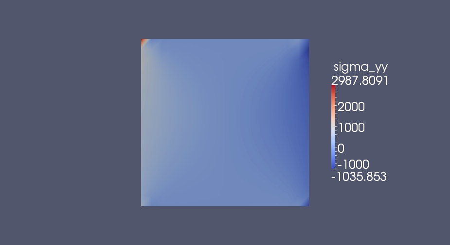
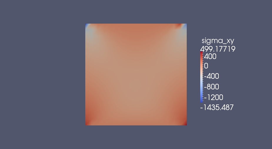
Fig. 2: Stress components $\sigma_{yy}$ and $\sigma_{xy}$ for $\mu_{E}=1$GPa, parameters $s=3,q=1.5,r=4$ and Flory-Huggins scaling parameter $10^{5}$Pa. Top row corresponds to fully permeable boundary and bottom row to impermeable.

 

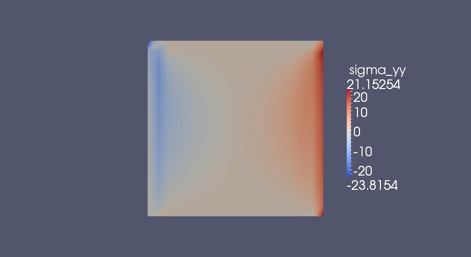
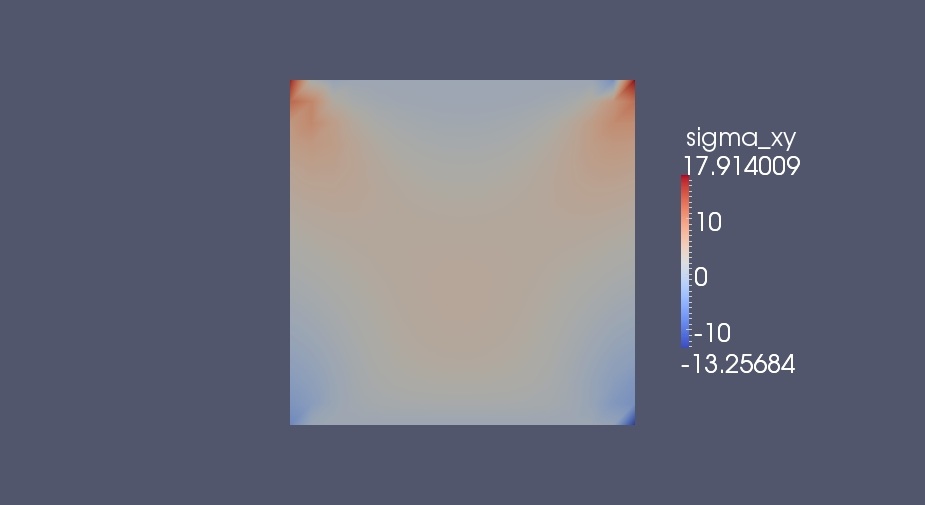
Fig. 3: Stress components $\sigma_{yy}$ and $\sigma_{xy}$ for $\mu_{E}=10^{9}$Pa, parameters $s=1,q=1.5,r=1.1$ and Flory-Huggins scaling parameter $10^{7}$Pa; fully permeable boundary.

We summarize the findings of our numerical simulations as follows.

1. The $\sigma_{yy}$ component presents stress concentration on the two fixed displacement edges, $\Gamma_{0}$, for the whole range of parameters that we tested. The components $\sigma_{xy}$ and $\sigma_{xx}$ (not included here) show corner concentration. In the case of impermeable boundary, the stress distributes almost uniformly across the domain, showing higher values than in the permeable case. Gels with permeable boundary show a low stress profile in the interior of the domain, with stresses concentrating on $\Gamma_{0}$.

2. The boundary stress concentrations of the $\sigma_{yy}$ component may trigger debonding upon reaching a experimentally determined threshold value [38].

3. For a given set of parameters, stresses in the case of impermeable boundary are higher than their permeable counterparts. This reflects the fact that, in a gel with fully permeable boundary, exchange of solvent takes place across the interface causing some stress relaxation. Moreover, in the ideal case of pure permeability, the fluid exchange takes place without loss of energy.

4. We have performed simulations with values of $s$ ranging from $s=1$ (Neo-Hookean material) to $s=3$ (hard rubber), and for values of $r$ ranging from $r=1.5$ (high compressibility) to $r=4$. We found that raising either of these exponents by 1, it may increase the stresses by at least by one order of magnitude.

5. The stress values, as represented by their maximum and minimum absolute values, show a decreasing pattern with the increase of the Flory-Huggins energy scaling with respect to the elastic one, reflecting softenning of the material.

6. The stresss distribution shown in the figures correspond to time equal to one hour. Calculations done for the same data after one day, show stress values in the same order of magnitude as the ones presented here.

7. Whereas the values of stresses shown in Figure 2 may be near the debonding pressure threshold, those in Figure 1 may have already crossed it. The experimental literature reports on values of the debonding pressure for different materials and loading conditions ranging from 0.5 to 10 times the elastic modulus $\mu_{E}$ [23].

8 Conclusions

We analyzed a model of the dynamics of gels that addresses inviscid and viscous solvent and polymer, permeability and traction-displacement boundary conditions, elasticity and diffusion. In particular, we focused on the linearized system about relevant equilibrium solutions and derived conditions for the solvability of the time dependent problems. These are also conditions that guarantee local stability of the equilibrium solutions of stress-free dilation and compression states as well as general equilibria, that is, solutions of traction-displacement boundary value problems of nonlinear elasticity. Although we proved well-posedness of the solutions of the time dependent equations linearized about dilation and compression states, the energy laws that we derived would allow us to extend the results to the more general linearized equations in a straight forward manner. In particular, the latter includes reference states with residual stress.

The analysis developed in this article answers specific questions arising in applications. Indeed, the assumptions ensuring stability of equilibrium solutions, and the subsequent well-posedness of the time dependent problem are formulated in terms of the parameters of the elastic and Flory-Huggins energies and their relative scale. Although this is far from sufficient to identify a material for a specific application, it does provide a criteria to eliminate materials for which instability would occur. This would have an immediate effect on reducing the number of costly and time consuming experiments to test a certain material for application by as much as 50 percent [25]. In addition to the stability characterization of the parameters, the numerical simulations provide data that indicate whether gel pressure has reached the debonding threshold. Furthermore, the choice of viscosity and drag coefficients determine the time of relaxation of a disturbance.

The simulations presented in the paper accurately address boundary conditions encountered in device applications, as well as values of elastic modulus $\mu_{E}=1GPa$ and Flory-Huggins parameters of realistic device materials. However, the domains that we use are two-dimensional and so, cannot represent realistic shapes of devices. Another important feature not addressed in the current research is the stress concentration phenomenon at the interface between two different materials of the device. Development of numerical tools based on Discontinuous Galerkin methods is currently underway to simulate actual devices more accurately.

The stress corner concentrations that we found have also been observed in gel membrane experiments on drug delivery devices. In this case, though, the presence of ions significantly magnifies the effect [32].

From a different point of view, a better understanding of the debonding phenomenon is needed, perhaps appealing to the problem of cavitation and cavity propagation. Experimental work on debonding also brings out the viscoelastic aspects of the phenomenon, so its treatment may require the adoption of viscoelastic stress strain laws [38].

The analysis presented here can be extended to treating triphasic models developed in the study of drug-delivery devices [34], [35]. However, this extension is not straightforward since the laws of balance of mass in the latter case are significantly more challenging.

From the point of view of analysis, one goal of the forthcoming work is to study the nonlinear problem within the context of the Oldroyd-B models of nonlinear elasticity. We point out that Sections 3.1.1 and 6 deal with the linearization of the system about arbitrary equilibrium solutions. This provides a necessary ingredient in the time discretization of a nonlinear model.

9 Acknowledgements

This work was partially supported by the National Science Foundation, grant number DMS 0909165. The authors also wish to extend their appreciation to Medtronic, Inc., Twin Cities, for the financial support and technical advice, especially by Dr. Suping Lyu, throughout the development of the project. The authors also wish to thank Professors Hans Weinberger, Francisco Javier Sayas, Bernardo Cockburn and Satish Kumar for the many useful discussions.

References

- [1] DOLFIN project http//www.fenics.org/dolfin.
- [2] J. M. Ball. Convexity conditions and existence theorems in nonlinear elasticity. Arch. Ration. Mech. Anal., 63:337–403, 1977.
- [3] L. S. Bennethum and J. H. Cushman. Multiscale, hybrid mixture theory for swelling systems–i: Balance laws. Int. J. Eng. Sci, 34:125–145, 1996.
- [4] L. S. Bennethum and J. H. Cushman. Multiscale, hybrid mixture theory for swelling systems–ii: Constitutive theory. Int. J. Eng. Sci, 34:147–169, 1996.
- [5] A. Boudaoud and S. Chaieb. Mechanical phase diagram of shrinking cylindrical gels. Phys. Rev. E, 68:021801, 2003.
- [6] A. Boudaoud and E. Sultan. The buckling of a swollen thin gel layer bound to a compliant substrate. J. Appl. Mech., 75:051002, 2008.
- [7] F. Brezzi. On the existence, uniqueness and approximation of saddle point problems arising from Lagrange multipliers. RAIRO Numerical Analysis, 8:129–151, 1974.
- [8] M. C. Calderer, B. Chabaud, S. Lyu, and H. Zhang. Modeling approaches to the dynamics of hydrogel swelling. Journal of Computational and Theoretical Nanoscience, -7(4), 2010.
- [9] M. C. Calderer and H. Zhang. Incipient dynamics of swelling of gels. SIAM J. Appl. Math., 68:1641–1664, 2008.
- [10] B. Chabaud. Models, analysis and numerics of gels. Univeristy of Minnesota,Ph.D thesis, 2009, 2009.
- [11] P.G. Ciarlet. Mathematical Elasticity, Vol 1. North-Holland, 1987.
- [12] C. M. Dafermos. A system of hyperbolic conservation laws with frictional damping. Z. Angew Math. Phys., 46:S294–S307, 1995.
- [13] C. M. Dafermos. Hyperbolic Conservation Laws in Continuum Physics. Springer, 2005.
- [14] M. Doi and A. Onuki. Dynamic coupling between stress and composition in polymer solutions and blends. J. Phys. II France, 2:1631–1656, 1992.
- [15] X. Feng and Y. He. Analysis of fully discrete finite element methods for a system of differential equations modeling swelling dynamics of polymer gels. Submitted, 2009.
- [16] P.J. Flory. Principles of Polymer Chemistry. Cornell U. Press, 1953.
- [17] D. R. Gaskell. Introduction to the Thermodynamics of Materials. Taylor & Francis, 1995.
- [18] G. Gatica and F.J. Sayas. Characterizing the inf-sup condition on product spaces. Numer. Math., 109:209–231, 2008.
- [19] V. Girault and P. A. Raviart. Finite Element Approximation of the Navier Stokes Equations. Number 749 in Lecture Notes in Mathematics. Springer Verlag, Berlin, Heidelbert, New York, 1979.
- [20] K.Micek H.Chen, Y.Mori and M.C.Calderer. A dynamic model of polyelectrolyte gels. SIAM J.Appl. Math, in press, 2012.
- [21] FEniCS Project. http://www.fenics.org. University of Chicago, Chalmers University and University of Oslo.
- [22] D. Kaiser. Coupling cell movement to multicellular development in myxobacteria. Nature Reviews Microbiology, 1:45–54, 2003.
- [23] K.R.Shull and C.Creton. Deformation behavior of thin, compliant layers under tensile loading conditions. J. Polymer Sci. Prg B: Polym, Phys., 42:4023–4073, 2004.
- [24] O. A. Ladyzhenskaya. The Mathematical Theory Of Viscous Incompressible Fluid. Gordon and Breach, 1969.
- [25] S. Lyu. Personal communication, 2010.
- [26] M.C. Calderer M. Rognes and C. Micek. Mixed finite element methods for gels with biomedical applications. SIAM J. Appl.Math, 70:1305–1329, 2009.
- [27] E. Fried M.E. Gurtin and L. Anand. Continuum Mechanics and Thermodynamics. Cambridge University Press, 2009.
- [28] M. A. Murad, L. S. Bennethum, and J. H. Cushman. Macroscale thermodynamics and the chemical potential of swelling porous media. Transport in Porous Media, 39:187–225, 2000.
- [29] A. Onuki. Theory of pattern formation in gels: Surface folding in highly compressible elastic bodies. Phys Rev A, 39:5932–5948, 1989.
- [30] H. Reichenbach and M. Dworkin. Introduction to the gliding bacteria. In The prokaryotes, pages 315–327, 1981.
- [31] F.J. Sayas. Personal communication, 2010.
- [32] R.A. Siegel. Personal communication, 2011.
- [33] R. Temam. The Navier-Stokes Equations: Theory and Numerical Analysis. 2nd edn. North-Holland, Amsterdam, 1977.
- [34] J. H. Cushman T.J. Weinstein and L. S. Bennethum. Two-scale, three-phase theory for swelling drug delivery systems. part i: Mixture theory. J.Pharm Sci, 97:1878–1903, 2008.
- [35] J. H. Cushman T.J. Weinstein and L. S. Bennethum. Two-scale, three-phase theory for swelling drug delivery systems. part ii: Flow and transport. J.Pharm Sci, 97:1904=1915, 2008.
- [36] C. Truesdell and W.Noll. The Non-Linear Field Theories of Mechanics. Springer Verlag, third edition, 2010.
- [37] J.Zhou W.Hong, X. Zhao and Z.Suo. A theory of coupled diffusion and large deformation in polymeric gels. J.Mech.Phys. Sol., 56:1779–1793, 2008.
- [38] T. Yamaguchi and M. Doi. Debonding dynamics of pressure-sensitive adhesives: 3d block model. Eur Phys J.E, 21:331–339, 2006.
- [39] T. Yamaue and M. Doi. Theory of one-dimensional swelling dynamics of polymer gels under mechanical constraint. Phys. Rev. E, 69:041402, 2004.
- [40] T. Yamaue, H. Mukai, K. Asaka, and M. Doi. Electrostress diffusion coupling model for polyelectrolyte gels. Macromolecules, 38:1349–1356, 2005.
- [41] T. Yamaue, T. Taniguchi, and M. Doi. The simulation of the swelling and deswelling dynamics of gels. Molecular Physics, 102(2):167–172, 2004.