Irradiation Induced Dimensional Changes in Bulk Graphite; The theory

Abstract

Basing on experimental data on irradiation-induced deformation of graphite we introduced a concept of diffuse domain structure developed in reactor graphite produced by extrusion. Such domains are considered as random continuous deviations of local graphite texture from the global one. We elucidate the origin of domain structure and estimate the size and the degree of orientational ordering of its domains. Using this concept we explain the well known radiation-induced size effect observed in reactor graphite. We also propose a method for converting the experimental data on shape-change of finite-size samples to bulk graphite. This method gives a more accurate evaluation of corresponding data used in estimations of reactor graphite components lifetime under irradiation.

1 Introduction

Employment of graphite as neutron moderator as well as construction material has a long history starting with the first reactor created by Enrico Fermi. Artificial reactor grade graphites were designed for these purposes[1]. The graphite components life time in active zone actually determines a life time of water-cooled carbon reactor as a whole, stimulating a study of radiation-induced evolution of reactor graphite properties.

With respect to production technology, reactor grade graphites range from almost isotropic to substantially anisotropic. Here we imply both physical and mechanical properties as well as irradiation effects. Widely used reactor grade graphites, such as Pile Grade A, ATR-2E, GR-280, produced by extrusion process exhibit a transversal-isotropic symmetry of physical and mechanical properties and radiation-induced effects[2, 3, 4, 5, 6, 7]. Such symmetry requires five independent mechanical constants; in different representations these are elasticity constants, or compliances, or the set of Young’s modulus, rigidity modulus, and Poisson coefficient[8].

Graphite rod subjected to irradiation undergoes transversely isotropic alternating-sign shape changes reaching several percent. The most important factors leading to non-uniform shape changes and hence, growth in internal stresses, are gradients of temperature and neutron exposure on the scale of a particular monolithic graphite element. Radiation-induced creep of graphite is not sufficient to compensate effects caused by shape changes and temperature gradients. Finally, a complicated irradiation-induced evolution of elastic moduli along with shape changes may lead, under low creep, to a destruction of monolithic graphite components.

In calculations of construction lifetime by using, e.g., the crack initiation and growth criterion, the determining factors are the data on evolution with neutron fluence of elastic moduli and relative shape changes in directions of an axis of symmetry (^∥) and in a plane of isotropy (^⟂)[2, 3, 4, 5, 6, 7, 9, 10, 11, 12]. The standard way to obtain such data is by irradiation of finite-size graphite samples in materials testing reactors at a higher, compared with power reactors, neutron flux accompanied with periodical measurements of characteristics. In 5-6 years the neutron fluence is acquired corresponding to 30-40 years lifetime graphite unit in operation conditions of power reactor. Such experiments are inevitably conducted under conditions different from operation ones, which has an inevitable influence on the data obtained. Necessary adjustments require a development of the corresponding models which would help to convert the data obtained under higher neutron flux for finite-dimension samples to conditions of bulk graphite and power reactors.

2 Formulation of the problem

In adjusting data on transversally isotropic reactor grade graphite irradiated in materials testing reactors one encounters three main problems, requiring a creation of models and a recalculation of corresponding data:

1. Differences in neutron energy spectra. The problem is sufficiently simply solved by standard methods of neutron fluence recalculation to solid-state doze values in terms of displacements per atom ($\operatorname{dpa}$) [5, 13]. Note that such conversion is not universal. When heterogeneous nucleation of microstructural elements is important (for example, PWR pressure vessels) the conversion to dpa results in a partial loss of needed information.

2. Noticeable differences in intensities of Frenkel pair generation ($\operatorname{dpa}/\operatorname*{s}$). Morphology of reactor grade graphite has a complicated multiscale structure formed by the filler, which comprises the objects with different degrees of order based on graphite micro-crystallites with the ideal crystal structure and dimensions of $\sim 10^{2}\operatorname{nm}$, a binder with an isotropic microcrystalline structure, and an ensemble of microcracks[1, 6, 9, 10, 11, 12, 14, 15]. By the objects are meant formations of various scales from micro-crystallite complexes with various packing to larger formations including grains. As the dimension scale increases, the objects become less anisotropic. An ensemble of microcracks is a result of relaxation processes at the scales with sufficiently high anisotropy level. At larger scales the anisotropy is too small to initiate the microcracks initiation.

   A driving force of radiation-induced effects in reactor grade graphite are processes taking place in an ideal crystalline structure of microcrystallite. Frenkel pair generation under the action of a neutron flux on crystal lattice results in the formation of a supersaturated two-component solid solution of interstitial atoms and vacancies. For a variety of reasons, the decay of quasi-2D supersaturated solid solution mainly leads to the formation of ensembles of interstitial dislocation loops of basal type, which, in turn, change microcrystallite shapes[6, 7, 12, 16]. Below we list current understanding of the microstructural mechanisms of radiation-induced shape changes of microcrystallites: The formation of interstitial clusters, dislocation loops and new graphitic planes will cause an expansion of the microcrystallite in the c-axis[17]. Adjacent lattice vacancies collapse parallel to the layers and form sinks for other vacancies, causing shrinkage parallel to the graphite layers[18]. Just the change of crystallite shape is a driving force for developing stresses, evolution of crack ensembles, and so on. At the bulk graphite scale, these effects are responsible for the shape changes, evolution of mechanical properties (partially) etc. Thus, juxtaposing radiation-induced effects obtained under different generation rates of Frenkel pairs ($\operatorname{dpa}/\operatorname*{s}$) requires solving the nontrivial problem on development of quasi-2D microstructure in graphite crystal lattice with microcrystal self-consistent boundary conditions[19].

3. Discrepancy between radiation-induced shape changes of bulk graphite and data obtained on finite-dimension samples. In our previous work [20], based on numerous measurements of shape changes in cylindrical samples the two results were obtained:

   Initially circular cross-section of the sample under irradiation takes an increasingly pronounced elliptical shape and orientations of the ellipses vary randomly along the sample on a scale of $0.6\operatorname{cm}$. The results of calculations of the relative volume changes using traditionally accepted methodology

   $$\left(\Delta V/V\right)_{T}=\left(\Delta L/L\right)^{\parallel}+2\left(\Delta L/L\right)^{\perp},$$ (1)

   (where $\left(\Delta L/L\right)^{\parallel}$ and $\left(\Delta L/L\right)^{\perp}$ are relative length changes of the samples cut from the bulk material in directions parallel and perpendicular to the extrusion direction) increasingly diverge with irradiation doze from the results of the direct measurements of the relative volume changes (see Fig. 1).

   

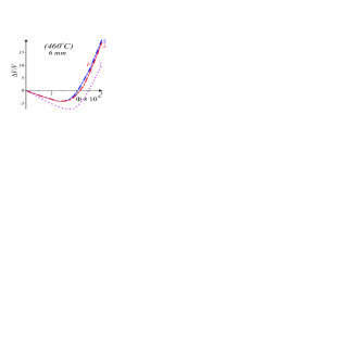
   Figure 1: Relative volume change $\Delta V/V$ (in %) as a function of fluence $\Phi$ ($\operatorname{neutrons}/\operatorname{m}^{2}$, $E_{n}>0.18\operatorname{MeV}$) in samples irradiated at temperature $460\pm 25^{\circ}\operatorname{C}$. Two dash-dotted lines are experimentally measured volumes $\Delta L/L+2\left(\Delta d/d\right)$ in $d=6\operatorname{mm}$ diameter cylindrical samples of length $L$ with both parallel (^∥) and perpendicular (^⟂) cuts relative to the extrusion direction; single dotted line ($T$) shows the traditionally used combination (1), calculated using longitudinal experimental data for those two extrusions. For the sample with $d=8\operatorname{mm}$, the result is qualitatively the same.

   As it was shown[20] the reason for such a mismatch is that expression (1) only relates the relative elongations of samples to relative volume change while neglecting changes in cross-sectional areas.

Basing on the presented experimental facts it was assumed that at macro-scale graphite can be considered as an transversally-isotropic elastic medium with irradiation-induced shape changes described by gradient tensor:

$$\hat{F}_{M}=\left(\begin{array}[c]{ccc}1+\left(\Delta L/L\right)^{\perp}&0&0\\ 0&1+\left(\Delta L/L\right)^{\perp}&0\\ 0&0&1+\left(\Delta L/L\right)^{\parallel}\end{array}\right).$$ (2)

Here, $\left(\Delta L/L\right)^{\parallel,\perp}$ are the relative bulk graphite shape changes in parallel and perpendicular directions relative to the axis of symmetry (which coincides with the extrusion direction). But on a scale of $\simeq 0.6\operatorname{cm}$, nonuniformities in shape changes are observed.

Actually, to such regions without pronounced boundaries may correspond local (at a scale of $l\simeq 0.6\operatorname{cm}$) random deviations of the axis of symmetry from the average direction in the bulk graphite. This representation was formalized by introducing a concept of “domain” – the region of size $l$ possessing the gradient tensor of relative radiation-induced deformation in local coordinate system

$$\hat{F}_{0}=\left(\begin{array}[c]{ccc}1+\left(\Delta l/l\right)_{\perp}&0&0\\ 0&1+\left(\Delta l/l\right)_{\perp}&0\\ 0&0&1+\left(\Delta l/l\right)_{\parallel}\end{array}\right).$$ (3)

Here $\left(\Delta l/l\right)_{\alpha}$ are irradiation-induced relative changes in sizes of free domain (i.e. mentially cut out of the elastic medium). The axis of symmetry of the domain is inclined at random angle $\theta$ with respect to that of bulk graphite (see Fig. 2).

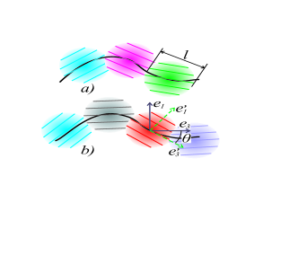
Figure 2: The random elastic medium with direction of anisotropy (solid line) continuously varying in space on the scale $l$ can be visualized in several equivalent ways a) and b) as the sets of diffuse domains of size $l$. The axis $\mathbf{e}_{3}^{\prime}$ (anisotropy direction) of local coordinate system $\left(\mathbf{e}_{1}^{\prime},\mathbf{e}_{2}^{\prime},\mathbf{e}_{3}^{\prime}\right)$ related to domains is rotated by random angle $\theta=\theta\left(\mathbf{x}\right)$ with respect to the axis $\mathbf{e}_{3}$ (orthotropy direction) of global coordinate system $\left(\mathbf{e}_{1},\mathbf{e}_{2},\mathbf{e}_{3}\right)$ related to the sample.

The domains are continuously transformed in space into each other on the scale of domain size $l$. It is impossible to uniquely identify the boundaries of such “diffuse” domains, which can be defined only statistically as regions in space with correlated directions of anisotropy.

The longitudinal measurement data $\left(\Delta L/L\right)^{\parallel},\left(\Delta L/L\right)^{\perp}$ can be calculated by averaging over random angle $\theta$ the projections of tensors $\hat{F}_{0}$ to the axis of symmetry of cylindrical samples. Such formalism leads us to writing a closed system of equations for obtaining $\left(\Delta l/l\right)_{\parallel},\left(\Delta l/l\right)_{\perp}$ and $\overline{\sin^{2}\theta}$, where $\theta$ is the angular deviation of the domain axis of symmetry from the bulk graphite common axis of symmetry, by using experimentally measured parameters $\left(\Delta L/L\right)_{S}^{\parallel},\left(\Delta L/L\right)_{S}^{\perp}$, and $\bar{\varepsilon}=\frac{1}{N}\sum\nolimits_{k=1}^{N}\varepsilon_{k}$ where $\varepsilon_{k}=\left[d_{\max}-\left(d_{\min}\right)_{k}\right]/d$ is the flattening factor for $k$-th transversal cross-section of the sample.

The developed model consistently explains the entire array of obtained experimental data. Taking into account that sample cross-sections are of the same scale ($d=0.6\operatorname{cm}$ and $d=0.8\operatorname{cm}$) as domain size, the irradiation-induced change of domain shape in samples can be considered as almost free dilatation (parameters $\left(\Delta l/l\right)_{\parallel}$ and $\left(\Delta l/l\right)_{\perp}$). At the same time, if we consider the case of radiation-induced effects in bulk graphite, the presence of an ensemble of disoriented domains with changing shapes would give rise to internal stresses, which entails a conclusion that shape and volume changes in bulk graphite are not equivalent to those in finite-size cylindrical samples. Keeping in mind that we are aimed at determining shape changes of bulk graphite while experimental data refer to samples with cross-sections on the same scale as the domains size, we have to recalculate the experimental data.

This work is devoted to further development of model [20] in order to suggest a method for recalculating data obtained on small-size samples to radiation-induced shape changes of bulk graphite. In the model developed for transversal-isotropic medium we employ pure elastic approach rather than elastoplastic one as required for rigorous solution of the problem. This is explained by insufficient understanding of the mechanisms of graphite irradiation creep related to the problem II above. Actually we obtain a lower bound for influence of disoriented domain structure on shape changes in bulk graphite.

In section 3 we develop a new approach to the description of elasticity of such diffuse domain structure. We consider both the case of high anisotropy (see Fig. 3 b) and uniform distribution of anisotropy directions (see Fig. 3 c).

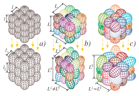
Figure 3: Domain structures in graphite: spherical shape of diffuse domains with transversely isotropic symmetry (shown by grid lines) and size $l$ becomes ellipsoidal (with sizes $l_{\perp}\neq l_{\parallel}$) due to irradiation-induced shape-change of free domains. Regular structure a) deforms affinely ($L^{\perp}/L^{\parallel}=l_{\perp}/l_{\parallel}$). The domains in irregular domain structure b) and c) randomly deform due to interaction with their elastic environment, and the structure as the whole deforms nonaffinelly ($L^{\perp}/L^{\parallel}\neq l_{\perp}/l_{\parallel}$): In case b) of high anisotropy the macroscopic deformation has the same transversely isotropic symmetry ($L^{\perp}\neq L^{\parallel}$), but different amplitude compared with the domains. In case c) of isotropic distribution of domain directions the macroscopic deformation is isotropic ($L^{\perp}=L^{\parallel}$) even for anisotropic domain deformation ($l_{\perp}\neq l_{\parallel}$).

Those cases correspond to different grades of reactor graphite[1, 4, 5, 6]. Macroscopic description of diffuse domain structure on scales large with respect to domain size is developed in section 4. In section 5 we describe formation of diffuse domain structure in graphite produced by the extrusion process. We also estimate size and a degree of alignment of the emerging domains.

3 Elasticity of diffuse domain structure

In this section we introduce main concepts and formulate a physical model of elasticity of diffuse domain structure. We consider diffuse domains as more or less homogeneous regions with anisotropic elasticity. Such domains do not have sharp boundaries, and their direction of anisotropy continuously and randomly change in space on scale of domain size $l$, see Fig. 2.

3.1 Strain of domain structure

Deformation of solid can be described by strain tensor $\hat{\varepsilon}$, which is related to the gradient tensor as $\hat{\varepsilon}=(\hat{F}\hat{F}^{T}-1)/2$, where ^T means transposition. Since the domain size is much larger than the scale of micro-cracks the strain tensor can be considered as a continuous function of coordinates ${\mathbf{x}}$. We describe deformation of graphite by taking the state before irradiation as reference state. Thus defined strain tensor can be presented as the sum $\hat{\varepsilon}^{tot}=\hat{\varepsilon}^{M}+\hat{\varepsilon}$ of two contributions: macroscopic deformation of sample $\hat{\varepsilon}^{M}\left({\mathbf{x}}\right)$ and local elastic deformation $\hat{\varepsilon}\left({\mathbf{x}}\right)$ with components

$$\varepsilon_{\alpha\beta}=\frac{1}{2}\left(\frac{\partial u_{\alpha}}{\partial x_{\beta}}+\frac{\partial u_{\beta}}{\partial x_{\alpha}}\right)$$ (4)

where $u_{\alpha}$ are components of elastic deformation vector. In equilibrium, this vector describes local deviations on the scale of domain size $l$, so that its average over the macro-scale vanishes.

In the case of bulk graphite with free boundaries the macroscopic strain tensor $\hat{\varepsilon}^{M}$ is diagonal in global coordinate system related to sample (see Fig. 2). In linear approximation in relative changes of sample sizes $\left(\Delta L/L\right)_{\alpha}$ in principal directions $\alpha=1,2,3$ (see Fig. 3 b) it can be written as

$$\varepsilon_{\alpha\beta}^{M}=\left(F_{M}\right)_{\alpha\beta}-\delta_{\alpha\beta}=\left(\Delta L/L\right)_{\alpha}\delta_{\alpha\beta}$$ (5)

Here and below, if possible, we shall drop the index $M$ characterizing the bulk graphite. Gradient tensor $\hat{F}_{M}$ is defined in Eq. (2) and $\delta$ is the unit Kronecker tensor.

Graphite domains are randomly oriented in space. The local coordinate system related to the domains (see Fig. 2 b) can be obtained from global coordinate system related to sample by means of rotations by three Euler angles $\Omega$: two polar angles $\varphi$ and $\psi$ and the azimuthal angle $\theta$, characterizing the orientation of the local frame with respect to the graphite orthotropy axis. All three angles $\Omega\left({\mathbf{x}}\right)=\left(\varphi\left({\mathbf{x}}\right),\theta\left({\mathbf{x}}\right),\psi\left({\mathbf{x}}\right)\right)$ randomly vary in space with coordinates ${\mathbf{x}}$ on the scale of domain size $l$. Domain rotation by given angles $\Omega=\left(\varphi,\theta,\psi\right)$ can be described by rotation matrix:

$$\begin{array}[c]{c}\hat{r}\left(\Omega\right)=\left(\begin{array}[c]{ccc}\cos\varphi&-\sin\varphi&0\\ \sin\varphi&\cos\varphi&0\\ 0&0&1\end{array}\right)\times\\ \left(\begin{array}[c]{ccc}1&0&0\\ 0&\cos\theta&-\sin\theta\\ 0&\sin\theta&\cos\theta\end{array}\right)\left(\begin{array}[c]{ccc}\cos\psi&-\sin\psi&0\\ \sin\psi&\cos\psi&0\\ 0&0&1\end{array}\right)\end{array}$$ (6)

This matrix relates the strain tensors in global $\hat{\varepsilon}^{tot}=\hat{\varepsilon}^{M}+\hat{\varepsilon}$ and in local $\hat{\varepsilon}^{loc}$ coordinate systems:

$$\varepsilon_{\alpha\beta}^{tot}=\sum\nolimits_{\alpha^{\prime}\beta^{\prime}}r_{\alpha\alpha^{\prime}}r_{\beta\beta^{\prime}}\varepsilon_{\alpha^{\prime}\beta^{\prime}}^{loc}$$ (7)

Eq. (7) can be rewritten in matrix notations as

$$\varepsilon_{i}^{tot}=\sum\nolimits_{j}R_{ij}\left(\Omega\right)\varepsilon_{j}^{loc}$$ (8)

Here and below we use Greek indexes ($\alpha\beta$) to distinguish components of symmetric tensor $\varepsilon_{\alpha\beta}=\varepsilon_{\beta\alpha}$ and Latin indexes ($i$) when presenting this tensor in vector notation. The first three components of such vector determine normal strain $\varepsilon_{i}=\varepsilon_{ii}$ ($i=1,2,3$) and the other three components of this vector determine shear strain, $\varepsilon_{4}=2\varepsilon_{23},\varepsilon_{5}=2\varepsilon_{13}$ and $\varepsilon_{6}=2\varepsilon_{12}$. Similar expressions for stress tensor are $\sigma_{i}=\sigma_{ii}$ ($i=1,2,3$) and $\sigma_{4}=\sigma_{23},\sigma_{5}=\sigma_{13},\sigma_{6}=\sigma_{12}$.

The rotation matrix $\hat{R}\left(\Omega\right)$ in Eq. (8) is

$$\begin{array}[c]{c}\hat{R}\left(\Omega\right)=\left(\begin{array}[c]{ccc}r_{11}^{2}&r_{12}^{2}&r_{13}^{2}\\ r_{21}^{2}&r_{22}^{2}&r_{23}^{2}\\ r_{31}^{2}&r_{32}^{2}&r_{33}^{2}\\ 2r_{21}r_{31}&2r_{22}r_{32}&2r_{23}r_{33}\\ 2r_{11}r_{31}&2r_{12}r_{32}&2r_{13}r_{33}\\ 2r_{11}r_{21}&2r_{12}r_{22}&2r_{13}r_{23}\end{array}\right.\\ \left.\begin{array}[c]{ccc}r_{13}r_{12}&r_{13}r_{11}&r_{11}r_{12}\\ r_{23}r_{22}&r_{23}r_{21}&r_{21}r_{22}\\ r_{33}r_{32}&r_{33}r_{31}&r_{31}r_{32}\\ r_{23}r_{32}+r_{22}r_{33}&r_{23}r_{31}+r_{21}r_{33}&r_{22}r_{31}+r_{21}r_{32}\\ r_{11}r_{32}+r_{11}r_{32}&r_{13}r_{31}+r_{11}r_{33}&r_{12}r_{31}+r_{11}r_{32}\\ r_{11}r_{22}+r_{12}r_{23}&r_{13}r_{21}+r_{11}r_{23}&r_{12}r_{21}+r_{11}r_{22}\end{array}\right)\end{array}$$

and where $r_{ij}$ are elements of the matrix (6). Below we use notations $\hat{R}^{-1}\left(\Omega\right),\hat{R}^{T}\left(\Omega\right)$ and $\hat{R}^{-T}\left(\Omega\right)$ for inverse, transposed and inverse transposed rotation matrixes, respectively.

3.2 Elastic energy of domain structure

Energy of diffuse domain structure takes simplest form in local coordinate system, which continuously rotates in space (see Fig. 2 b):

$$E=\dfrac{1}{2}\int d{\mathbf{x}}{{\displaystyle\sum\nolimits_{ij}}}c_{ij}\left[\hat{\varepsilon}^{loc}\left({\mathbf{x}}\right)-\hat{\varepsilon}^{F}\right]_{i}\left[\hat{\varepsilon}^{loc}\left({\mathbf{x}}\right)-\hat{\varepsilon}^{F}\right]_{j}$$ (9)

Irradiation-induced dilatation of freely dilating domains $\hat{\varepsilon}^{F}$ describes irreversible deformation of the domain with free boundaries (which was cut out of the sample) due to irradiation. The dilatation is diagonal in local coordinate system related to the domain:

$$\varepsilon_{\alpha\beta}^{F}=\left(\hat{F}_{0}\right)_{\alpha\beta}-\delta_{\alpha\beta}=\left(\Delta l/l\right)_{\alpha}\delta_{\alpha\beta}$$ (10)

Here $\hat{F}_{0}$ is defined in Eq. (3) and $\left(\Delta l/l\right)_{\alpha}$ are corresponding relative changes of free domain sizes in principal directions $\alpha=1,2,3$, see Fig. 3 a. The strain in local coordinate system $\hat{\varepsilon}^{loc}\left({\mathbf{x}}\right)$ is related to the strain $\hat{\varepsilon}$ in global coordinate system via Eqs. (7) and (8). Notice, that the above defined strain tensors have different origination: $\hat{\varepsilon}^{F}$ (Eq. 10) describes irreversible irradiation induced domain dilatation and creep, $\hat{\varepsilon}$ is truly elastic deformation tensor and the macroscopic deformation $\hat{\varepsilon}^{M}$ (Eq. 5) has both inelastic and elastic contributions.

Symmetric stiffness matrix $\hat{c}$ in Eq. (9) is nearly the same for all domains, but the axis of its symmetry randomly rotates with respect to direction of bulk graphite orthotropy axis. Components $c_{ij}$ of local stiffness matrix $\hat{c}$ are elastic moduli of the domain. They change under irradiation and depend on neutron fluence and temperature (see section 6 below). Here we consider the case of transversely isotropic symmetry, when the matrix $\hat{c}$ in local coordinate system has the form

$$\hat{c}=\left(\begin{array}[c]{cccccc}c_{11}&c_{12}&c_{13}&0&0&0\\ c_{12}&c_{11}&c_{13}&0&0&0\\ c_{13}&c_{13}&c_{33}&0&0&0\\ 0&0&0&c_{44}&0&0\\ 0&0&0&0&c_{44}&0\\ 0&0&0&0&0&\left(\allowbreak c_{11}-c_{12}\right)/2\end{array}\right)$$ (11)

Substituting the local strain $\hat{\varepsilon}^{loc}$ from Eq. (8) to elastic energy (9) we finally get elastic energy of diffuse domain structure

$$E=\dfrac{1}{2}{\displaystyle\int}d{\mathbf{x}{\displaystyle\sum\nolimits_{ij}}}c_{ij}\left[\hat{R}^{-1}\left(\hat{\varepsilon}+\hat{\varepsilon}^{M}\right)-\hat{\varepsilon}^{F}\right]_{i}\left[\hat{R}^{-1}\left(\hat{\varepsilon}+\hat{\varepsilon}^{M}\right)-\hat{\varepsilon}^{F}\right]_{j}$$ (12)

Using this elastic energy we describe below in section 4.4 three the most important cases of domain structures:

Regular:

Regular structure (see Fig. 3 a) deforms affinely with domain deformation. In this case the equilibrium macroscopic deformation is the same as for free domains, Eq. (10), $\hat{\varepsilon}^{M}=\hat{\varepsilon}^{loc}=\hat{\varepsilon}^{F}$.

Free:

In the case of “unconnected” freely dilated domains $\hat{\varepsilon}^{loc}=\hat{\varepsilon}^{F}$ and the macroscopic deformation $\hat{\varepsilon}^{M}=\overline{\hat{R}}\hat{\varepsilon}^{F}$ differs from deformation of individual domains $\hat{\varepsilon}^{F}$ only due to difference in domain orientations. Here the bar means averaging over domain orientation.

Irregular:

Domains of irregular structure (see Fig. 3 b) are in more cramped conditions with respect to the case of regular domain structure. Elastic environment tends to compress the domain with respect to the case of freely dilated domains and $\hat{\varepsilon}^{loc}\neq\hat{\varepsilon}^{F}$. Equilibrium deformation $\hat{\varepsilon}^{M}$ is determined by balance between elastic deformation of the domain and elastic response of its environment on this deformation.

Uniform:

In the case of uniform distribution of domain directions (see Fig. 3 c) the macroscopic deformation $\hat{\varepsilon}^{M}$ is isotropic even for strongly anisotropic deformation of individual domains, $\hat{\varepsilon}^{loc}\neq\hat{\varepsilon}^{F}$.

4 Macroscopic description of diffuse domain structure

In this section we develop macroscopic theory of reactor graphite elasticity. Although diffuse domains have different orientations, many such domains at spatial scales large with respect to domain size form an orthotropic and homogeneous material from a marcomechanics standpoint. The main feature of diffuse domain structure is absence of cross-domain boundaries, near which the breakup of stress or strain may take place as in ordinary polycristalline solids. In the case of diffuse domain structure both stress and strain change continuously and the domains of diffuse domain structure directly feel the stress $\hat{\sigma}\left({\mathbf{x}}\right)$ of the elastic enviroment. Under the influence of such stress the randomly turned domains deform non-affinely with macroscopic deformation of bulk graphite (see Fig. 3 b and c) and the strain $\hat{\varepsilon}$ of such irregular domain structure gains large short wavelength (on the order of domain size $l$) components.

4.1 Local stress

Elastic energy (12) can be expanded in powers of the strain $\hat{\varepsilon}$. We leave linear term in this expansion unchanged, and transform only its quadratic term using the equality

$$\begin{array}[c]{c}\dfrac{1}{2}{\displaystyle\int}d{\mathbf{x}{\displaystyle\sum\nolimits_{ij}}}c_{ij}\left(\hat{R}^{-1}\hat{\varepsilon}\right)_{i}\left(\hat{R}^{-1}\hat{\varepsilon}\right)_{j}=\\ -\dfrac{1}{2}{{\displaystyle\int}}d{\mathbf{x}{\displaystyle\sum\nolimits_{ij}}}S_{ij}\sigma_{i}\sigma_{j}+{{\displaystyle\int}}d{\mathbf{x}{\displaystyle\sum\nolimits_{i}}}\sigma_{i}\varepsilon_{i}\end{array}$$ (13)

Here

$$\hat{S}\left(\Omega\right)=\hat{R}\left(\Omega\right)\hat{s}\hat{R}^{T}\left(\Omega\right)$$ (14)

is local compliance matrix in global coordinate system and $\hat{s}=\hat{c}^{-1}$ is local compliance matrix inverse to the local stiffness matrix $\hat{c}$, Eq. (11). Let us show that if the stress $\hat{\sigma}$ is found from extremum of the right hand side of Eq. (13), the latter will be equal to the left hand side of this equation. Substituting the solution of extremum equation for the local stress

$$\sigma_{i}=\sum\nolimits_{j}S_{ij}^{-1}\left(\Omega\right)\varepsilon_{j}=\sum\nolimits_{j}\left[\hat{R}^{-T}\left(\Omega\right)\hat{c}\hat{R}^{-1}\left(\Omega\right)\right]_{ij}\varepsilon_{j}$$ (15)

back to the right hand side of Eq. (13) we really reproduce the expression for the left hand side of this equation.

Using Eq. (13) we can transform quadratic in $\hat{\varepsilon}$ term in Eq. (12) into corresponding linear term and rewrite elastic energy (12) in terms of the local stress $\hat{\sigma}\left({\mathbf{x}}\right)$:

$$E\left[\sigma\right] =const-\dfrac{1}{2}\int d{\mathbf{x}}\sum\nolimits_{ij}S_{ij}\left[\Omega\left({\mathbf{x}}\right)\right]\sigma_{i}\left({\mathbf{x}}\right)\sigma_{j}\left({\mathbf{x}}\right)+$$

$$\int d{\mathbf{x}}{\displaystyle\sum\nolimits_{i}}\left(\sigma_{i}\left({\mathbf{x}}\right)+\sigma_{i}^{M}\left[\Omega\left({\mathbf{x}}\right)\right]-\sigma_{i}^{F}\left[\Omega\left({\mathbf{x}}\right)\right]\right)\varepsilon_{i}\left({\mathbf{x}}\right)$$ (16)

where $\hat{\sigma}^{F}$ is stress because of irradiation-induced deformation of the domain. In matrix notations

$$\sigma_{i}^{F}\left[\Omega\left({\mathbf{x}}\right)\right]=\hat{R}^{-T}\left(\Omega\right)\hat{c}\hat{\varepsilon}^{F}$$ (17)

Stress $\hat{\sigma}^{M}$ describes elastic response of medium on this deformation:

$$\hat{\sigma}^{M}\left(\Omega\right)=\hat{R}^{-T}\left(\Omega\right)\hat{c}\hat{R}^{-1}\left(\Omega\right)\hat{\varepsilon}^{M}=\hat{S}^{-1}\left(\Omega\right)\hat{\varepsilon}^{M}$$ (18)

Minimum of elastic energy (16) gives standard equation of equilibrium in the presence of external stress $\sigma_{i}\left({\mathbf{x}}\right)$:

$${\displaystyle\sum\limits_{\beta}}\frac{\partial}{\partial x_{\beta}}\left(\sigma_{\alpha\beta}+\sigma_{\alpha\beta}^{M}-\sigma_{\alpha\beta}^{F}\right)=0$$ (19)

To derive this equation we substituted elastic strain (4) in Eq. (16). Variation of elastic energy for given stress tensor $\hat{\sigma}$ takes the form

$$\delta E=\int d{\mathbf{x}}{\displaystyle\sum\nolimits_{\alpha\beta}}\left(\sigma_{\alpha\beta}+\sigma_{\alpha\beta}^{M}-\sigma_{\alpha\beta}^{F}\right)\frac{\partial\delta u_{\alpha}}{\partial x_{\beta}}$$

Integrating this expression by parts and equating volume term to zero, we find Eq. (19).

The solution of this linear equation can be written as a superposition of contributions from all domains. Each of these contributions slowly decays with the distance from the domain (as a power law at large distances). The domains have random orientations, and their total contribution to the stress is effectively self-averaged because of discussed above long-range character of elasticity. Therefore, in deriving equations of macroscopic elasticity we may consider the stress $\hat{\sigma}\left({\mathbf{x}}\right)$ as weakly varying on the scale of domain size function. Since angles $\Omega$ randomly alter in space, the constant stress $\hat{\sigma}$ describes strain $\hat{\varepsilon}\left({\mathbf{x}}\right)$ strongly varying in space on the scale of domain size, see Eq. (15).

Note that Eq. (19) corresponds to minimum of energy (16). Because of this minimum condition substitution of the approximate solution $\hat{\sigma}\left({\mathbf{x}}\right)\simeq const$ of stochastic equation (19) in energy (16) gives only minor corrections of second order in small-scale space variations of the function $\hat{\sigma}\left({\mathbf{x}}\right)$.

4.2 Derivation of macroscopic elasticity equations

Below we will neglect the effect of weak spatial stress variations on the scale of domain size $l$ on macroscopic elasticity of graphite. Than the integration over ${\mathbf{x}}$ in Eq. (16) is equivalent to pre-averaging of the stress expansion coefficients $S_{ij}\left[\Omega\left({\mathbf{x}}\right)\right],\sigma_{i}^{M}\left[\Omega\left({\mathbf{x}}\right)\right]$ and $\sigma_{i}^{F}\left[\Omega\left({\mathbf{x}}\right)\right]$ over characteristic spatial scale of the function $\hat{\sigma}\left({\mathbf{x}}\right)$, and macroscopic free energy for slowly varying stress $\hat{\sigma}\left({\mathbf{x}}\right)$ takes the form

$$\begin{array}[c]{c}E\left[\sigma\right]=-\dfrac{1}{2}{{\displaystyle\int}}d{\mathbf{x}{\displaystyle\sum\nolimits_{ij}}}\bar{S}_{ij}\sigma_{i}\left({\mathbf{x}}\right)\sigma_{j}\left({\mathbf{x}}\right)\\ +{{\displaystyle\int}}d{\mathbf{x}{\displaystyle\sum\nolimits_{i}}}\left[\sigma_{i}\left({\mathbf{x}}\right)+\bar{\sigma}_{i}^{M}\left({\mathbf{x}}\right)-\bar{\sigma}_{i}^{F}\left({\mathbf{x}}\right)\right]\varepsilon_{i}\left({\mathbf{x}}\right),\end{array}$$ (20)

where bar means averaging over space.

Equation of equilibrium (19) can also be transferred to its pre-averaged form with the aid of equality

$$\begin{array}[c]{c}\overline{\dfrac{\partial F\left({\mathbf{x}}\right)}{\partial x_{\beta}}}={{\displaystyle\int}}d{\mathbf{x}}^{\prime}w\left({\mathbf{x}}^{\prime}-{\mathbf{x}}\right)\dfrac{\partial F\left({\mathbf{x}}^{\prime}\right)}{\partial x_{\beta}^{\prime}}=-{{\displaystyle\int}}d{\mathbf{x}}^{\prime}\dfrac{\partial w\left({\mathbf{x}}^{\prime}-{\mathbf{x}}\right)}{\partial x_{\beta}^{\prime}}F\left({\mathbf{x}}\right)\\ =\dfrac{\partial}{\partial x_{\beta}}{{\displaystyle\int}}d{\mathbf{x}}^{\prime}w\left({\mathbf{x}}^{\prime}-{\mathbf{x}}\right)F\left({\mathbf{x}}^{\prime}\right)=\dfrac{\partial\bar{F}\left({\mathbf{x}}\right)}{\partial x_{\beta}}\end{array}$$

which is valid for any function $F\left({\mathbf{x}}\right)$ and bell-like weight function $w\left({\mathbf{x}}^{\prime}-{\mathbf{x}}\right)$. The weight function is centered at point ${\mathbf{x}}$ and has characteristic size larger than $l$. As the result of such averaging Eq. (19) for slowly varying stress $\hat{\sigma}\left({\mathbf{x}}\right)$ takes the form

$$\sum\limits_{\beta}\frac{\partial}{\partial x_{\beta}}\left[\sigma_{\alpha\beta}\left({\mathbf{x}}\right)+\bar{\sigma}_{\alpha\beta}^{M}\left({\mathbf{x}}\right)-\bar{\sigma}_{\alpha\beta}^{F}\left({\mathbf{x}}\right)\right]=0$$ (21)

In equilibrium neighbouring domains can self-consistently adapt their deformations since rigid directions of these domains are deployed by random angles to each other. Eq. 21 should be solved with the boundary conditions on surface of bulk sample:

$$\sum\nolimits_{\beta}\left[\sigma_{\alpha\beta}\left({\mathbf{x}}\right)+\bar{\sigma}_{\alpha\beta}^{M}\left({\mathbf{x}}\right)\right]n_{\beta}=P_{\alpha}$$ (22)

where $n_{\beta}$ are components of normal to the surface, and $P_{\alpha}$ are components of external force applied to the surface. This force can be considered as a substitute at the surface of corresponding volume source of deformation $\bar{\sigma}_{\alpha\beta}^{F}$ in Eq. 21.

Elastic energy (20) can be rewritten in standard form of macroscopic theory of elasticity by introducing “smoothed” on the domain scale $l$ strain tensor $\bar{\varepsilon}$ with components

$$\bar{\varepsilon}_{i}\left({\mathbf{x}}\right)=\sum\nolimits_{j}\bar{S}_{ij}\sigma_{j}\left({\mathbf{x}}\right)$$ (23)

which is obtained by averaging the microscopic strain $\hat{\varepsilon}$ with the above weight function $w$:

$$\begin{array}[c]{c}\bar{\varepsilon}_{i}\left({\mathbf{x}}\right)={\displaystyle\int}d{\mathbf{x}}^{\prime}w\left({\mathbf{x}}^{\prime}-{\mathbf{x}}\right)\varepsilon_{i}\left({\mathbf{x}}^{\prime}\right)\\ ={\displaystyle\int}d{\mathbf{x}}^{\prime}w\left({\mathbf{x}}^{\prime}-{\mathbf{x}}\right){{\displaystyle\sum\nolimits_{j}}}S_{ij}\left[\Omega\left({\mathbf{x}}^{\prime}\right)\right]\sigma_{j}\left({\mathbf{x}}^{\prime}\right)\\ \simeq{\displaystyle\int}d{\mathbf{x}}^{\prime}w\left({\mathbf{x}}^{\prime}-{\mathbf{x}}\right){{\displaystyle\sum\nolimits_{j}}}S_{ij}\left[\Omega\left({\mathbf{x}}^{\prime}\right)\right]\sigma_{j}\left({\mathbf{x}}\right)=\sum_{j}\bar{S}_{ij}\sigma_{j}\left({\mathbf{x}}\right)\end{array}$$

Substituting Eq. (23) into elastic energy (20) we can rewrite it in standard form for macroscopic elasticity:

$$E\left[\bar{\varepsilon}\right] ={\displaystyle\int}d{\mathbf{x}}\left[\dfrac{1}{2}{{\displaystyle\sum\nolimits_{ij}}}\bar{C}_{ij}\bar{\varepsilon}_{i}\left({\mathbf{x}}\right)\bar{\varepsilon}_{j}\left({\mathbf{x}}\right)+\right.$$

$$\left.{{\displaystyle\sum\nolimits_{i}}}\left(\bar{\sigma}_{i}^{M}\left({\mathbf{x}}\right)-\bar{\sigma}_{i}^{F}\left({\mathbf{x}}\right)\right)\bar{\varepsilon}_{i}\left({\mathbf{x}}\right)\right]$$ (24)

where $\bar{C}=\bar{S}^{-1}$ is macroscopic stiffness matrix, $\bar{\sigma}_{i}^{F}\left({\mathbf{x}}\right)$ and $\bar{\sigma}_{i}^{M}\left({\mathbf{x}}\right)$ are averages of the corresponding values (17) and (18). Minimum of this energy reproduces equation of equilibrium of effective elastic medium (21), where the stress $\hat{\sigma}$ is related to the strain $\bar{\varepsilon}$ via Eq. (23). Since we defined $\hat{\varepsilon}^{M}$ as equilibrium macroscopic strain (see Eq. 5) in equilibrium we have $\sigma_{\alpha\beta}\left({\mathbf{x}}\right)=\bar{\varepsilon}_{\alpha\beta}\left({\mathbf{x}}\right)=0$. Eq. (24) with $\bar{\varepsilon}_{\alpha\beta}\left({\mathbf{x}}\right)\neq 0$ describing elastic response of graphite to external perturbation (elastic moduli, see next section).

4.3 Elastic moduli of bulk sample

The average compliance matrix $\bar{S}$ in Eq. (20) is found by space averaging the local compliance matrix $\hat{S}\left(\Omega\right)$, Eq. (14):

$$\bar{S}_{ij}=\sum\nolimits_{kl}\overline{R_{ik}\left(\Omega\right)R_{jl}\left(\Omega\right)}s_{kl}$$ (25)

Averaging of inverse stiffness matrix, and not of stiffness matrix itself, is related to the fact that domains deform non-affinely with the macroscopic strain, see Fig. 3 b[25]. Instead, they directly feel the applied macroscopic stress $\hat{\sigma}\left({\mathbf{x}}\right)$[26].

Space averaging in Eqs. (20) and (25) can be rewritten as averaging over all orientations of domains $\Omega=\left(\varphi,\theta,\psi\right)$. Rotation angles $\varphi$ and $\psi$ are randomly distributed in the interval $\left(0,2\pi\right)$ while probability distribution of the azimuthal angle $\theta$ can be characterized by the second and fourth moments of $\sin\theta$:

$$m_{2}=\int_{0}^{\pi/2}\sin^{2}\theta\Psi\left(\theta\right)\sin\theta d\theta,\quad m_{4}=\int_{0}^{\pi/2}\sin^{4}\theta\Psi\left(\theta\right)\sin\theta d\theta$$ (26)

The distribution function $\Psi\left(\theta\right)$ of the angle $\theta$ is calculated below in section 5.2 in case of graphite manufactured through the process of extrusion. In this case the fourth moment $m_{4}$ can be expressed in terms of the second moment $m_{2}$, see Eq. 45 below.

Calculating the angular average in Eq. (25) we get linear relation between elements of averaged and local compliance matrixes:

$$\bar{S}_{11} =s_{11}+\tfrac{1}{2}\left(-2s_{11}+2s_{13}+s_{44}\right)m_{2}+\tfrac{3}{8}s,$$

$$\bar{S}_{12} =s_{12}+\left(-s_{12}+s_{13}\right)m_{2}+\tfrac{1}{8}s,$$

$$\bar{S}_{13} =s_{13}+\tfrac{1}{2}\left(s_{11}+s_{12}-3s_{13}+s_{33}-s_{44}\right)m_{2}-\tfrac{1}{2}s,$$ (27)

$$\bar{S}_{33} =s_{33}+\left(2s_{13}-2s_{33}+s_{44}\right)m_{2}+s,$$

$$\bar{S}_{44} =s_{44}+\tfrac{1}{2}\left(6s_{11}-2s_{12}-8s_{13}+4s_{33}-5s_{44}\right)m_{2}-2s,$$

$$s =\left(s_{11}-2s_{13}+s_{33}-s_{44}\right)\allowbreak m_{4}$$

In case of uniform distribution of domain directions $\Psi\left(\theta\right)=1$ substituting the moments

$$m_{2}=2/3,\qquad m_{4}=8/15$$ (28)

into the above equations we obtain moduli of macroscopically isotropic material (see Fig. 3 c):

$$\bar{S}_{11} =\bar{S}_{33}=\tfrac{1}{15}\left(8s_{11}+4s_{13}+3s_{33}+2s_{44}\right),$$

$$\bar{S}_{12} =\bar{S}_{13}=\tfrac{1}{15}\left(s_{11}+5s_{12}+8s_{13}+s_{33}-s_{44}\right),$$ (29)

$$\bar{S}_{44} =2\left(\bar{S}_{11}-\bar{S}_{12}\right)=\tfrac{2}{15}\left(7s_{11}-5s_{12}-4s_{13}+2s_{33}+5s_{44}\right)$$

Anisotropy and degree of disorientation increase with decreasing spatial scale and become large on scale of a stack of microcrystallites. Under the effect of thermal expansion of microcrystallites amplitude of stress on this scale can reach the level of crack initiation and growth. The characteristic scale of emerging microcracks is small compared to domain size. Therefore, relation (27) between macroscopic and domain modules do not depend on evolution of microcrack subsystem and is determined only by the distribution of domain orientations.

4.4 Free boundary conditions

Solution of Eq. (21) for samples subjected to external pressure $P$ is $\bar{\sigma}^{M}-\bar{\sigma}^{F}=\hat{\sigma}^{ext}$ with diagonal tensor $\sigma_{\alpha\beta}^{ext}=P\delta_{\alpha\beta}$. In case of free boundary conditions there is no stress at the boundary of the sample, $\hat{\sigma}^{ext}=0$, and the equilibrium macroscopic strain $\hat{\varepsilon}^{M}$ is determined by the condition of zero average stress:

$$\bar{\sigma}^{M}=\bar{\sigma}^{F}$$ (30)

This condition corresponds to equilibrium between the average stress due to irradiation-induced deformation of domains, Eq. (17) and the average stress due to response of elastic medium on this deformation, Eq. (17). Averaging the local stresses, Eqs. (17) and (18), over Euler angles $\Omega=\left(\psi,\phi,\theta\right)$ we find linear matrix equation for the macroscopic strain (5):

$$\overline{\hat{S}^{-1}\left(\Omega\right)}\hat{\varepsilon}^{M}=\overline{\hat{R}^{-T}\left(\Omega\right)}\hat{c}\hat{\varepsilon}^{F}$$

The solution of this equation is

$$\left(\Delta L/L\right)^{\parallel} =\left(\Delta l/l\right)_{\parallel}+k^{\parallel}\left[\left(\Delta l/l\right)_{\perp}-\left(\Delta l/l\right)_{\parallel}\right],$$

$$\ \left(\Delta L/L\right)^{\perp} =\left(\Delta l/l\right)_{\perp}-\tfrac{1}{2}k^{\perp}\left[\left(\Delta l/l\right)_{\perp}-\left(\Delta l/l\right)_{\parallel}\right]$$ (31)

The factors $k$ in this expression can be written in explicit form:

$$k^{\parallel} =\left[2\left(4c_{44}c_{\parallel}-\Delta\right)\allowbreak m_{2}+\left(c_{\perp}-c_{\parallel}\right)\allowbreak\gamma m_{2}^{2}\right.$$

$$\left.\left.+2c_{\parallel}\left(\gamma-4c_{44}\right)\allowbreak m_{4}\right]\right/K,$$ (32)

$$k^{\perp} =\left[2\left(4c_{44}c_{\perp}-\Delta\right)m_{2}+2\left(c_{\parallel}-c_{\perp}\right)\left(\gamma+c_{\perp}-c_{\parallel}\right)\allowbreak m_{2}^{2}\right.$$

$$\left.\left.+2c_{\perp}\left(\gamma-4c_{44}\right)\allowbreak m_{4}\right]\right/K,$$ (33)

$$K =2\Delta+\left[4c_{44}\left(c_{\perp}+2c_{\parallel}\right)-6\Delta\right]\allowbreak m_{2}-\left(c_{\perp}-c_{\parallel}\right)^{2}m_{2}^{2}$$

$$+\allowbreak\left(c_{\perp}+2c_{\parallel}\right)\left(\gamma-4c_{44}\right)\allowbreak\allowbreak m_{4}$$

where $m_{2}$ and $m_{4}$ are moments of $\sin\theta$ (see Eq. 26) and we use abbreviations

$$\begin{array}[c]{ll}c_{\parallel}=c_{11}+c_{12}+c_{13},&c_{\perp}=2c_{13}+c_{33},\\ \gamma=c_{11}+c_{12}-2c_{13},&\Delta=c_{33}\left(c_{11}+c_{12}\right)-2c_{13}^{2}\end{array}$$

Combining Eqs. (31) we find radiation-induced change of sample volume

$$\Delta V/V =\left(\Delta L/L\right)^{\parallel}+2\left(\Delta L/L\right)^{\perp}$$

$$= \left(\Delta l/l\right)_{\parallel}+2\left(\Delta l/l\right)_{\perp}-k_{V}\left[\left(\Delta l/l\right)_{\perp}-\left(\Delta l/l\right)_{\parallel}\right],$$ (34)

Amplitude of volume change is described by the factor $k_{V}$:

$$k_{V} =k^{\perp}-k^{\parallel}=\left(c_{\perp}-c_{\parallel}\right)\left[8c_{44}m_{2}-\left(3\gamma+2c_{\perp}-2c_{\parallel}\right)m_{2}^{2}\right.$$

$$\left.\left.+2\left(\gamma-4c_{44}\right)m_{4}\right]\right/K$$ (35)

In case $k_{V}=0$ ($c_{\perp}=c_{\parallel}$) the relative volume change is the same as for medium with freely dilating domains

$$\left(\Delta V/V\right)_{F}=\left(\Delta l/l\right)_{\parallel}+2\left(\Delta l/l\right)_{\perp}$$

although such sample deforms strongly anisotropically (see Fig. 3 b). In case $k_{V}\neq 0$ the difference between those volume changes is related to deformation of domain shape due to elastic response of environment. The case $k_{V}>0$ corresponds to compression of the domain by the medium, and $k_{V}<0$ describes its dilation.

Consider most important cases in more detail:

Regular:

Regular domain structure corresponds to case $m_{2}=m_{4}=0$, when the macroscopic strain coincides with the irradiation-induced strain,

$$\left(\Delta L/L\right)^{\parallel}=\left(\Delta l/l\right)_{\parallel},\qquad\left(\Delta L/L\right)^{\perp}=\left(\Delta l/l\right)_{\perp}$$

The bulk sample deforms affinely with domain deformation, see Fig. 3 a.

Free:

Stress in freely dilated domains is determined by the local condition $\hat{\sigma}^{M}\left({\mathbf{x}}\right)=\hat{\sigma}^{F}\left({\mathbf{x}}\right)$ that does not satisfy the equilibrium equation (19) due to long-range character of elasticity. The solution $\hat{\varepsilon}^{M}\left({\mathbf{x}}\right)=\hat{R}\left[\Omega\left({\mathbf{x}}\right)\right]\hat{\varepsilon}^{F}$ of the above condition takes into account only domain rotation and ignores elastic response of the medium on irradiation-induces deformation of domains. Below for comparison we write down macroscopic deformation of such fictional medium of freely dilating objects:

$$\ \left(\Delta L/L\right)_{F}^{\parallel} =\left(\Delta l/l\right)_{\parallel}+m_{2}\left[\left(\Delta l/l\right)_{\perp}-\left(\Delta l/l\right)_{\parallel}\right]$$

$$\left(\Delta L/L\right)_{F}^{\perp} =\left(\Delta l/l\right)_{\perp}-\tfrac{1}{2}m_{2}\left[\left(\Delta l/l\right)_{\perp}-\left(\Delta l/l\right)_{\parallel}\right]$$ (36)

and corresponding volume change of such medium:

$$\left(\frac{\Delta V}{V}\right)_{F}=\left(\frac{\Delta L}{L}\right)_{F}^{\parallel}+2\left(\frac{\Delta L}{L}\right)_{F}^{\perp}=\left(\frac{\Delta l}{l}\right)_{\parallel}+2\left(\frac{\Delta l}{l}\right)_{\perp}$$ (37)

Irregular:

At high anisotropy of domain directions (see Fig. 3 b) the factors $k$ are proportional to the second moment $m_{2}\ll 1$:

$$k^{\parallel}\simeq\left(4c_{44}c_{\parallel}/\Delta-1\right)m_{2},\quad k^{\perp}\simeq\left(4c_{44}c_{\perp}/\Delta-1\right)m_{2}$$ (38)

Nonaffine deformation of bulk sample is related both to random rotation of domains and elastic response of the medium on their shape-change. To separate both contributions compare Eqs. (31) and (38) with Eqs. (36). The factors $k^{\parallel}$ and $k^{\perp}$ are both proportional to $m_{2}$, and similarly to Eq. (36) they take into account the effect of domain disorientation on sample size. The difference between $k^{\parallel},k^{\perp}$ and $m_{2}$ is due to compression of domains by their elastic environment.

Uniform:

In case of uniform distribution of domain directions (see Fig. 3 c) with moments (28) we find from Eqs. (32) and (33) that the sample as the whole deforms isotropically under irradiation:

$$\begin{array}[c]{c}\left(\Delta L/L\right)^{\parallel}=\left(\Delta L/L\right)^{\perp}=\\ \dfrac{c_{\perp}}{c_{\perp}+2c_{\parallel}}\left(\dfrac{\Delta l}{l}\right)_{\parallel}+\dfrac{2c_{\parallel}}{c_{\perp}+2c_{\parallel}}\left(\dfrac{\Delta l}{l}\right)_{\perp}\end{array}$$

5 Formation of diffuse domain structure

In this section we propose simple model of diffuse domains formation in graphite prepared by direct melt extrusion process. We also estimate the size of such domains and describe orientational alignment of domains in extrusion flow.

5.1 Typical domain size $l$

We will treat a mixture of pitch and coke particles at fabrication conditions as very viscous incompressible fluid. Velocity field ${\mathbf{v}}({\mathbf{x}})$ of such fluid with density $\rho$ can be described by Navier-Stokes equation:

$$\rho\left[\partial{\mathbf{v}}/\partial t+\left({\mathbf{v}}\triangledown\right){\mathbf{v}}\right]-\eta\triangledown^{2}{\mathbf{v=f}}$$ (39)

with boundary condition ${\mathbf{v}}=0$ at channel walls. Here $\triangledown$ is gradient, $\eta$ is dynamic viscosity of the fluid and force ${\mathbf{f}}$ initiates rotation of random graphite crystallites. Before extrusion the crystallites have random directions of anisotropy (with uniform distribution function $\Psi_{0}\left(\theta\right)=1$), and they are rotated in the flow under influence of gradient of the force ${\mathbf{f}}$. Mechanism of such rotation is different on spatial scales small and large with respect to characteristic correlation length

$$l{\mathbf{\simeq\operatorname{Re}}}\eta/\left(\rho v\right)$$ (40)

where $\operatorname{Re}$ is effective Reynolds number:

At small scales $x<l$

main contribution to left hand side of Eq. (39) comes from viscous term $-\eta\triangledown^{2}{\mathbf{v\simeq f}}$. This term stabilizes the flow inside the correlation volume $l^{3}$ and describes regular laminar motion of the fluid on the scale $l$. Therefore, the rotation of anisotropy axes due to the force ${\mathbf{f}}$ is strongly correlated at small spatial scales $x<l$.

At large scales $x>l$

main contribution to the turning force ${\mathbf{f}}$ comes from the term $\rho\left({\mathbf{v}}\triangledown\right){\mathbf{v\simeq f}}$, which describes convective acceleration (instability) of the flow and leads to randomization of motion at large distances $x>l$ due to amplification of the effect of random initial orientation of crystallites. This amplification also leads to a decrease in the Reynolds number $\operatorname{Re}$ with respect to case of ordinary structureless fluid.

Using characteristic Reynolds number $\operatorname{Re}\simeq 10$ we find from Eq. (40) a simple estimate of domain size for viscous fluid with typical kinematic viscosity $\nu=\eta/\rho\simeq 100\operatorname{cSt}$ ($\operatorname{mm}^{2}/\operatorname{s}$) and average velocity of flow $v\simeq 10\operatorname{cm}/\operatorname{s}$:

$$l\simeq\operatorname{Re}\nu/v\simeq 1\operatorname{cm}$$ (41)

This estimation is in good agreement with domain size $l\simeq 0.6\operatorname{cm}$ observed in GR-280 graphite[20]. Although our estimate of the Reynolds number $\operatorname{Re}$ needs additional experimental justification, Eq. (41) can be used to predict flow temperature and velocity gradient dependence of the domain size $l$ in reactor graphites.

5.2 Distribution of domain orientations

Due to random shape and orientations of crystallites the turning force ${\mathbf{f}}$ in Eq. (39) is also random, and coarse-grained at scale $l$ domains in the flow experience rotations at random angles $\delta\theta$ during a small time interval $\delta t$, see Fig. 4.

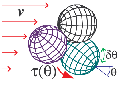
Figure 4: Randomly turned coarse-grained at scale $l$ domains rotate in the gradient flow $\mathbf{v}\left(\mathbf{x}\right)$ at random angles $\delta\theta$ during a small time interval $\delta t$ and are oriented under the influence of orientation-dependent torque $\tau\left(\theta\right)$.

Such diffusion-like rotations can be described by orientational Smoluchowski equation for distribution function $\Psi\left(\theta\right)$ of domain angles $\theta$:

$$\frac{\partial\Psi\left(\theta\right)}{\partial t}=\frac{1}{\sin\theta}\frac{\partial}{\partial\theta}\left\{D\left(\theta\right)\sin\theta\left[\frac{\partial\Psi\left(\theta\right)}{\partial\theta}+\tau\left(\theta\right)\Psi\left(\theta\right)\right]\right\}$$ (42)

with uniform initial distribution $\Psi_{0}\left(\theta\right)=1$ before extrusion. In general, the angular diffusion coefficient $D\left(\theta\right)=\left\langle\delta\theta^{2}\right\rangle/(2\delta t)$ can depend on the angle $\theta$. The drift term in this equation reflects the fact that the domain experiences an average torque $\tau\left(\theta\right)$ due to the flow, which restricts its free rotation. Both opposite directions of domain anisotropy are equivalent, $\tau\left(\pi-\theta\right)=\tau\left(\theta\right)$ and therefore, the expansion of this function in a Fourier series has the form:

$$\tau\left(\theta\right)=\sum\nolimits_{n>0}\tau_{n}\sin\left(2n\theta\right).$$

Higher order corrections $\tau_{n}$ with $n>1$ are not important for our consideration and will be dropped below. Amplitude $\tau=\tau_{1}$ of the dimensionless torque is proportional to average strain rate of the flow.

Steady state solution of Eq. (42) at times $t\gg D^{-1}$ has the form

$$\Psi\left(\theta\right)=e^{\tau\cos^{2}\theta-g\left(\tau\right)},\qquad g\left(\tau\right)=\ln\left(\int_{0}^{\pi/2}e^{\tau\cos^{2}\theta}\sin\theta d\theta\right)$$ (43)

Substituting the distribution function (43) in Eq. (26) we find expressions for first two moments of this distribution:

$$m_{2}=1-g^{\prime}\left(\tau\right),\qquad m_{4}=m_{2}^{2}+g^{\prime\prime}\left(\tau\right)$$ (44)

In case of graphite obtained by extrusion at large velocity gradients the torque $\tau$ is large, $\tau\gg 1$, and we get from Eq. (44) $m_{2}\simeq 1/\tau\ll 1$ and $m_{4}\simeq 2m_{2}^{2}$. In case of graphite formed under hydrostatic pressure average torque is small, $\tau\ll 1$, and we reproduce moments of uniform distribution, Eq. (28). A typical value of the second moment of graphite GR-280 $m_{2}\simeq 0.3$ corresponds to intermediate case $\tau\simeq 4$ between those two limits.

In the Ref.[20] we show that the second moment $m_{2}$ can be directly obtained from analysis of experiments measuring irradiation-induced deformation of small size graphite samples. The fourth moment $m_{4}$ can be expressed in terms of the second moment $m_{2}$ excluding parameter $\tau$ from Eqs. (44). Implicit dependence (44) of the fourth moment on the second moment can be interpolated for the whole range of torque $\tau>0$ by the following simple expression:

$$m_{4}\simeq\frac{\allowbreak 2m_{2}^{2}}{1+3m_{2}^{2}/2}$$ (45)

6 Dose dependence

Compliance moduli of a domain $s_{ij}$ can be estimated using experimentally measured macroscopic compliance moduli $\bar{S}_{ij}$. Difficulties in determining a set of five independent constants $\bar{S}_{ij}$ characterizing elastic properties of transversely isotropic solid lie in the fact that, as a rule, only two Young’s modules $E_{\parallel},E_{\perp}$ and Poisson’s ratio $\nu$ are investigated in studies of irradiation effects of reactor graphite. In our case, we need to know all the five independent constants as well as their dose dependence.

Experimental data for non-irradiated Pile Grade A reactor graphite[28] are shown in Table 1.

Pile	$\bar{S}_{11}$	$\bar{S}_{12}$	$\bar{S}_{13}$	$\bar{S}_{33}$	$\bar{S}_{44}$
Grade A	$2.150$	$-0.127$	$-0.123$	$1.087$	$3.333$
Mono-	$s_{11}^{m}$	$s_{12}^{m}$	$s_{13}^{m}$	$s_{33}^{m}$	$s_{44}^{m}$
crystal	$0.011$	$-0.00045$	$-0.025$	$0.326$	$4.35$
Domain	$s_{11}$	$s_{12}$	$s_{13}$	$s_{33}$	$s_{44}$
	$2.\,\allowbreak 5$	$-0.12$	$-0.19$	$0.64$	$2.73$

Table 1: Compliance moduli of Pile Grade A [28] and monocrystal non-irradiated graphites (in units of $10^{-11}\operatorname{cm^{2}/dyn}$). In last raw we show our estimate for domain complience moduli.

We expect that this graphite forms macroscopically homogeneous domain structure similarly to GR-280 graphite, since both of them are fabricated by the same extrusion method (see section 5 above). Values of moments $m_{2}$ and $m_{4}$ and domain size $l$ for these graphites may differ.

Effect of irradiation on elasticity of Pile Grade A graphite has been studied in details only for two Young’s moduli $E_{\parallel},E_{\perp}$ and Poisson’s ratios $\nu_{\parallel}$ and $\nu_{\perp}$ which are related to the macroscopic compliance moduli as[22, 23]:

$$\begin{array}[c]{llllll}E_{\parallel}&\!\!\!\!=1/\bar{S}_{33},&G_{\parallel}&\!\!\!\!=1/\bar{S}_{44},&\nu_{\parallel}&\!\!\!\!=-\bar{S}_{13}/\bar{S}_{33},\\ E_{\perp}&\!\!\!\!=1/\bar{S}_{11},&G_{\perp}&\!\!\!\!=1\left/\left[2\left(\bar{S}_{11}-\bar{S}_{12}\right)\right]\right.,&\nu_{\perp}&\!\!\!\!=-\bar{S}_{12}/\bar{S}_{11}.\end{array}$$

Dose dependence of entire set of compliance moduli has been established only for monocrystalline and pyrolytic graphites over a wide temperature range[29, 24, 30]. It is noticed that only “small” elastic constants $c_{33}$ and $c_{44}$ experience significant changes (increase in value) with irradiation dose.

Detailed data processing for the elastic moduli $E_{\parallel}$ and $E_{\perp}$ of ATR-2E graphite produced by extrusion, is given in Ref. [13]. It is shown that dose dependence of both Young’s moduli $E_{\parallel}$ and $E_{\perp}$ is the same. The only difference is in normalization factors:

$$E_{\parallel}\left(\Phi\right)=E_{\parallel}f\left(\Phi\right),\qquad E_{\perp}\left(\Phi\right)=E_{\perp}f\left(\Phi\right)$$ (46)

Functional dependence of structure factor $f\left(\Phi\right)$ on neutron fluence $\Phi$ is shown in Fig. 5 for different irradiation temperatures.

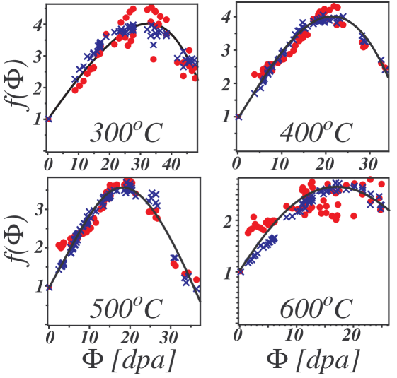
Figure 5: Dose $\Phi$ (in units of displacements per atom) dependence $f\left(\Phi\right)=E\left(\Phi\right)/E\left(0\right)$ of elastic moduli[13] of ATR-2E graphite at irradiation temperatures $300^{\circ},400^{\circ},500^{\circ}$ and $600^{\circ}C$ (circles). Crosses show the approximation of the function $f\left(\Phi\right)$ by Eq. (47).

Different experiments demonstrate similar shape of dose dependence of the elastic moduli: a rather sharp increase, reaching maximum and subsequent decrease. Below we propose simple empirical expression for dose dependence of the structure factor $f\left(\Phi\right)$.

We assume that there are two main contributions to the structure factor:

$$f\left(\Phi\right)\simeq 1-\vartheta\left(\Delta V/V\right)+\Phi/\Phi^{\ast}$$ (47)

due to evolution of subsystem of microcracks and due to irradiation hardening of crystallites. It is shown in Ref. [14] (Eq. 8) that the first of these contributions to elastic moduli is proportional to relative volume change $\Delta V/V$. This contribution is responsible for reversal of graphite shrinkage at high irradiation doses $\Phi$[14, 20]. Second contribution linearly grows with the irradiation dose $\Phi$ (different powers of $\Phi$ give worse agreement with experiments). As one can see from Fig. 5 this simple dependence (47) describes adequately well all main features of dose dependence of the elastic moduli at different irradiation temperatures. Note also that the two fitting constants $\vartheta\simeq 17$ and $\Phi^{\ast}\simeq 17$ almost do not depend (at noise level) on irradiation temperature. The universality of these constants is a further argument in support of equation (47). Large value of dimensionless constant $\vartheta$ is related to high contrast between elastic contributions of crystallites and microcracks. Similar correlations between dimensional change and Young’s modulus structure factor $f\left(\Phi\right)$ were also established for Gilsocarbon[27].

In order to determine dose dependence of all other elastic moduli, we first compare the Young’s modulus $E_{\parallel,\perp},G_{\parallel,\perp}$ and $\nu_{\parallel,\perp}$ for a typical Pile Grade A and single-crystal non-irradiated graphites, see Table 2.

Pile	$E_{\parallel}^{(a)}$	$G_{\parallel}^{(a)}$	$E_{\perp}^{(c)}$	$G_{\perp}^{(c)}$	$\nu_{\perp}$	$\nu_{\parallel}$
Grade A	$9.2$	$3.0$	$4.6$	$2.2$	$0.06$	$0.11$
Mono-	$E_{\perp}^{(a)}$	$G_{\perp}^{(a)}$	$E_{\parallel}^{(c)}$	$G_{\parallel}^{(c)}$	$\nu_{\perp}$	$\nu_{\parallel}$
crystal	$909$	$437$	$30$	$2.29$	$0.04$	$0.076$

Table 2: Young’s ($E$) and shear ($G$) moduli of Pile Grade A [28] and single-crystal non-irradiated graphites in units of $\operatorname{GPa}=10^{10}\operatorname{dyn}$ and corresponding Poisson’s ratios ($\nu$). Superscripts show preferential directions of crystal axes.

Due to random orientation of crystallites main contribution to all macroscopic moduli $\bar{S}_{ij}$ comes from “large” monocrystalline moduli $s_{33}^{m}$ and $s_{44}^{m}$ (see section 4.3 for description of orientational disorder effect). Macroscopic compliance moduli $\bar{S}_{ij}$ are only weakly affected by “small” moduli $s_{11}^{m},s_{12}^{m}$ and $s_{13}^{m}$ (see Table 1 for relative values of all moduli) since probability of finding basal planes along the direction of extrusion is small enough. In addition, anisotropy of elastic properties of reactor graphite is significantly smoothed out due to the presence of microcrack subsystem and binder[15]. The above described effects are responsible for observation of only moderate level of macroscopic orthotropy of graphite elasticity along with sharply pronounced anisotropy on crystallite scale.

We conclude that dose dependence of the shear moduli of diffuse domain structure (see Fig. 2) can be approximated by the same structure factor $f\left(\Phi\right)$ as for Young’s modules (46):

$$G_{\parallel}\left(\Phi\right)=G_{\perp}f\left(\Phi\right),\qquad G_{\perp}\left(\Phi\right)=G_{\perp}f\left(\Phi\right)$$ (48)

An important consequence of Eqs. (46) and (48) for the Poisson’s ratios

$$\nu_{\parallel}\left(\Phi\right)=const,\qquad\nu_{\perp}\left(\Phi\right)=const$$

is confirmed experimentally[28]. Using Eqs. (46) and (48) we find dose dependence of all macroscopic compliance moduli:

$$\bar{S}_{ij}\left(\Phi\right)=\bar{S}_{ij}f^{-1}\left(\Phi\right)$$

where $\bar{S}_{ij}$ are corresponding values of those moduli in absence of irradiation, see Table 1.

Knowing experimental values of the moduli $\bar{S}_{ij}$ Eqs. (27) can be solved for the domain compliance moduli $s_{ij}$

$$s_{ij}\left(\Phi\right)=s_{ij}f^{-1}\left(\Phi\right)$$ (49)

Calculated values $s_{ij}$ in the absence of irradiation for Pile Grade A graphite are also presented in Table 1. Substituting Eq. (49) into Eqs. (32), (33) and (35) and using experimental value $m_{2}\simeq 0.3$ and for GR-280 graphite[20] we estimate the factors

$$k^{\parallel}\simeq-0.17,\quad k^{\perp}\simeq 0.18,\quad k_{V}\simeq 0.35$$ (50)

in Eqs. (31) and (34) for relative shape changes of bulk graphite samples. We conclude that bulk graphite sample deforms nonaffinally with domain deformation.

Values of irradiation-induced dilatations $\left(\Delta l/l\right)_{\parallel}$ and $\left(\Delta l/l\right)_{\perp}$ can be estimated measuring deformation of cylindrical samples (S) with diameter $8$ mm close to the domain size $l$. Relative changes in length of such samples with orientations coinciding (^∥) and orthogonal (^⟂) to the extrusion direction are[20]:

$$\left(\Delta L/L\right)_{S}^{\parallel,\perp}=\left(\Delta l/l\right)_{\parallel}+m_{2}^{\parallel,\perp}\left[\left(\Delta l/l\right)_{\perp}-\left(\Delta l/l\right)_{\parallel}\right]$$ (51)

Here $m_{2}^{\parallel}\simeq 0.3$ and $m_{2}^{\perp}\simeq 0.7$ are second moments of corresponding samples irradiated at temperature $550^{\circ}$C.

Experimentally observed dose dependence of the relative length changes is plotted in Fig. 6. Using these data and substituting the solution $\left(\Delta l/l\right)_{\parallel,\perp}$ of Eqs. (51) into Eq. (31) we also plot the predicted dose dependence of relative elongations of macroscopic samples.

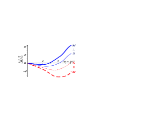
Figure 6: Dose dependence of relative deformations (in %) of graphite irradiated at temperature $T=550^{\circ}$C in reactor BOR-60$:$ The relative changes of the length of cylindric finite-size samples (S) and of macroscopic size samples (M) with orientations coinciding ($\parallel$, solid lines) and orthogonal ($\perp$, dashed lines) to the extrusion direction.

Note, that relative elongation of bulk samples is much higher than that of small size samples. In bulk samples the domains are in more crowded conditions in directions perpendicular to the extrusion direction (in these directions the deformation of domains due to orientational disorder is maximal). Therefore, at low doses, the relative strain in these directions is weaker, $|\Delta L/L|^{\perp}_{M}<|\Delta L/L|^{\perp}_{S}$. Increase in logitudinal strain $|\Delta L/L|^{\parallel}_{M}>|\Delta L/L|^{\parallel}_{S}$ is related to interaction between longitudinal and transverse elastic modes. These conditions can also be rewritten in a form $(\Delta L/L)^{\perp}_{M}>(\Delta L/L)^{\perp}_{S}$ and $(\Delta L/L)^{\parallel}_{M}<(\Delta L/L)^{\parallel}_{S}$ that is also valid for large doses. Since obtained results are sensitive to value of the moment $m_{2}$, it is desirable to carry out further experiments to get better characterization of reactor grade graphites texture.

7 Summary

The main results of this paper are as follows:

1. Basing on experimental data on radiation-induced deformation of graphite, we introduced the concept of diffuse domain structure, which is the reason of size effects in reactor graphite. In such structure there are no sharp boundaries between domains, and the direction of domain anisotropy undergoes random deviations from global orientation of the sample. We also derived equations of macroscopic elasticity, describing the deformation of solids due to irradiation-induced shape change of their domains having transversely isotropic structure. This theory can also be used to describe deformation of stressed samples. A relation is obtained between elastic moduli of domains and macroscopic solid as the whole. We have proposed a scheme for conversion of experimental data obtained on samples of finite size to describe shape-change of bulk graphite. Such scheme is required for engineering calculations of graphite blocks integrity.

2. We have presented simple model explaining origin of diffuse domains in graphite produced by the extrusion process. Our estimation of domain size is in good agreement with known experimental data[20]. This model can also be used to predict the dependence of the domain size on extrusion velocity and viscosity of visco-plastic medium.

3. We also elaborated simple model describing orientational ordering of domains during extrusion. This model enables us to calculate the moments of domain’s orientation, needed in description of elastic properties of reactor-grade graphite.

References

- [1] John H.W. Simmons, Radiation damage in graphite, Oxford, Pergamon Press (1965).
- [2] B.T. Kelly, W.H. Martin and P.T. Nettley, Phyl. Trans. A, 260 (1966).
- [3] B.T. Kelly, Prog. Nucl. Energy, 2 (1978) 219-269.
- [4] Irradiation damage in graphite due to fast neutrons in fission and fusion systems, IAEA-TECDOC-1154, September (2000).
- [5] G. Haag, Properties of ATR-2E Graphite and property changes due to fast neutron irradiation, Forschungszentrum, Jülich, (2005).
- [6] Ya.I. Shtrombakh, B.A. Gurovich, P.A. Platonov and V.M. Alekseev, J. of Nucl. Mater., 225 (1995) 273-301.
- [7] G. Hall, B.J. Marsden, S.L. Fok, J. Smart, Nucl. Engin. and Design, 222 (2003) 39-330.
- [8] J.F. Nye, Physical properties of crystals, Oxford, Clarendon Press, (1964).
- [9] D.K.L. Tsang, B.J. Marsden, J. of Nucl. Mater., 350 (2006) 208-220.
- [10] G. Hall, B.J. Marsden, S.L. Fok, J. of Nucl. Mater., 353 (2006) 12-18.
- [11] C. Berre et al. J. of Nucl. Mater., 352 (2006) 1-5.
- [12] T.D. Burchell, Proc. IAEA Specialist’s Meeting on the Present Status of Graphite Development for Gas-Cooled Reactors, Sept. 9 (1991) 49-58.
- [13] A.V. Subbotin, O.V. Ivanov, I.M. Dremin et al. Atomic Energy, 100 (2005) 204-26.
- [14] S.V. Panyukov and A.V. Subbotin, Atomic Energy, 105 (2008) 25-32.
- [15] S.V. Panyukov and A.V. Subbotin, Atomic Energy, 107 (2009) 268-273.
- [16] W.N. Reynolds and P.A. Thrower, Phyl. Mag. 12 (1965) 573-593.
- [17] S. Amelinckx, P. Delavignette and M. Heerschap, Dislocations and stacking faults in graphite, Chem. Phys. Carbon, ed. P.L. Walker 1 (1965) 1-71.
- [18] T.D. Burchell and T. Oku, Material properties data for fusion reactor plasma facing carbon-carbon composites Atomic and Plasma–Material Interaction Data for Fusion (supplement to J. Nucl. Fusion) 5 (1994) 77-128 (International Atomic Energy Agency).
- [19] W.C. Morgan, Carbon, 1 (1964) 255-261, 51-62.
- [20] M.V. Arjakov, A.V. Subbotin, S.V. Panyukov et al, J. of Nucl. Mater., 420 (2012) 241-251.
- [21] R.E. Nightingale and E.M. Woodruff, Nucl. Sci. and Engineering, 19 (1964) 390-392.
- [22] A.E.H. Love, Mathematical theory of elasticity, London, (1952).
- [23] S.G. Lekhnitsky, Elastic theory of anisotropic medium, Nauka, Moscow, 1977 (in Russian).
- [24] C. Baker and A. Kelly, Phil. Mag. 9 (1964), 927.
- [25] W. Voigt, Wied. Ann. 38 (1889) 573–587.
- [26] A. Reuss, Z. Angew. Math. Mech. 9 (1929) 49–58.
- [27] B.J. Marsden, G.N. Hall, Compr. Nucl. Mat., 4 (2012) 325-390.
- [28] Irradiation damage in graphite due to fast neutrons in fission and fusion systems, IAEA-TECDOC-1154, September (2000).
- [29] E.J. Seldin and C.W. Nezbeda, J. Appl. Phys. 41 (1970) 3389.
- [30] J.B. Ayasse and E. Bonjour, Pro. fourth SCI Conference on industrial carbons and graphites, SCI, London, (1976).