Relation between squeezing of vacuum fluctuations, quantum entanglement and sub-shot noise in Raman scattering

Abstract

A completely quantum description of Raman process is used to investigate the nonclassical properties of the modes in the stimulated, spontaneous and partially spontaneous Raman process. Both coherent scattering (where all the initial modes are coherent) and chaotic scattering (where initial phonon mode is chaotic and all the other modes are coherent) are studied. Nonclassical character of Raman process is observed by means of intermodal entanglement, single mode and intermodal squeezing of vacuum fluctuations, sub-shot noise and wave variances. Joint photon-phonon number and integrated-intensity distributions are then used to illustrate the observed nonclassicalities. Conditional and difference number distributions are also provided to illustrate the nonclassical character. The mutual relation between the obtained nonclassicalities and their variations dependent on phases, rescalled time and ratio of coupling constants are also reported.

Anirban Pathak^a,b, Jaromir ${\rm K}\breve{{\rm r}}{\rm epelka}^{b}$ and Jan ${\rm\check{Perina}}$^b,c

^aJaypee Institute of Information Technology, A-10, Sector-62, Noida, UP-201307, India

^bRCPTM, Joint Laboratory of Optics of Palacky University and Institute of Physics of Academy of Science of the Czech Republic, Faculty of Science, Palacky University, 17. listopadu 12, 771 46 Olomouc, Czech Republic

^cDepartment of Optics, Palacky University, 17. listopadu 12, 771 46 Olomouc, Czech Republic

Keywords: Raman scattering, nonclassicality, quasidistribution.

1 Introduction

Quantum statistics of Raman scattering were discussed from various points of view in a number of papers (see [1, 2] and references therein, Section 10.4 of [3] and [4] for reviews). In this paper we describe the Raman scattering process with a completely quantum mechanical Hamiltonian. The model is capable to include the stimulated, spontaneous and partially spontaneous Raman process. We use the second order short-time approximation for solution of the Heisenberg equation of motion corresponding to this Hamiltonian. The solution is then used to relate the nonclassical properties of photons and phonons in these processes (i.e. stimulated, spontaneous and partially spontaneous Raman process). To be precise, nonclassical characteristics of photon and phonon modes generated in these processes are exhibited through a number of properties, including squeezing of vacuum fluctuations, quantum entanglement of modes, sub-shot noise and wave variances. Further, joint photon-phonon number, integrated-intensity distributions, conditional and difference number distributions are also found useful to illustrate the observed nonclassicalities.

Remaining part of the paper is arranged as follows. In Section 2 we briefly describe the fully quantum Hamiltonian of Raman process and several criteria of nonclassicalities that are used in the present study. In Section 2 we have briefly described the model Hamiltonian that provides a completely quantum description of the Raman scattering process and also describe a normal-ordered characteristic function in the Gaussian form for the same system. Criteria for testing of nonclassicalities are also introduced. In Section 3 we investigate nonclassical character of Raman process for coherent scattering by means of intermodal entanglement, single mode and intermodal squeezing of vacuum fluctuations, sub-shot noise and wave variances. In Section 4 the same nonclassical characteristics are investigated for the chaotic scattering. The observed nonclassicalities are further illustrated through joint photon-phonon number and wave distribution in Section 5. In Section 6 we study difference and conditional number distributions associated with the Raman process. Finally, Section 7 is dedicated to conclusion.

2 The model Hamiltonian and the criteria of nonclassicality

A fully quantum description of the Raman scattering process can be provided by the following Hamiltonian [1, 5]:

$$H=\sum_{j=L,S,A,V}\hbar\omega_{j}a_{j}^{\dagger}a_{j}-\left(\hbar ga_{L}a_{S}^{\dagger}a_{V}^{\dagger}+\hbar\chi^{*}a_{L}a_{V}a_{A}^{\dagger}+{\rm h.c.}\right),$$ (1)

where ${\rm h.c.}$ stands for Hermitian conjugate and the subscripts $L,S,A$ and $V$ correspond to pump (laser), Stokes, anti-Stokes and vibration (phonon) modes respectively, $\omega_{j},\,a_{j}$ and $a_{j}^{\dagger}$ are frequency, annihilation operator and creation operator in the $j$ th mode, $g$ and $\chi$ are the Stokes and anti-Stokes coupling constants. Using the Hamiltonian (1) we can construct a set of Heisenberg equations and solve them in short-time approximation. A second order short-time approximated solution was already reported [3]. It is interesting to note that using the short-time approximated solution, we can obtain a normal-ordered characteristic function in the Gaussian form. Such a characteristic function can completely characterize the Raman process, and it can be analytically expressed as [3]

$$\begin{array}[]{lcl}C_{N}(\beta_{L},\beta_{S},\beta_{A},\beta_{V},t)&=&\left\langle\exp\left\{\sum_{j=L,S,A,V}\right.\left[-B_{j}(t)|\beta_{j}|^{2}\right.\right.\\ &+&\left.\left(\frac{1}{2}C_{j}^{*}(t)\beta_{j}^{2}+{\rm c.c.}\right)+\beta_{j}\xi_{j}^{*}(t)-\beta_{j}^{*}\xi_{j}(t)\right]+\\ &+&\left.\left.\sum_{j<k}\left(D_{jk}(t)\beta_{j}^{*}\beta_{k}^{*}+\bar{D}_{jk}(t)\beta_{j}\beta_{k}^{*}+{\rm c.c.}\right)\right\}\right\rangle,\end{array}$$ (2)

where ${\rm c.c.}$ stands for complex conjugate terms, the set $(L,\,S,\,A,\,V)$ is assumed to be ordered and

$$\begin{array}[]{lcl}B_{L}(t)&=&|\chi|^{2}t^{2}|\xi_{A}|^{2},\\ B_{S}(t)&=&|g|^{2}t^{2}|\xi_{L}|^{2},\\ B_{A}(t)&=&0,\\ B_{V}(t)&=&|g|^{2}t^{2}|\xi_{L}|^{2}+|\chi|^{2}t^{2}|\xi_{A}|^{2},\\ C_{L}(t)&=&-g^{*}\chi t^{2}\xi_{S}\xi_{A}\exp(-2i\omega_{L}t),\\ C_{S}(t)&=&0,\\ C_{A}(t)&=&0,\\ C_{V}(t)&=&-g\chi t^{2}\xi_{S}^{*}\xi_{A}\exp(-2i\omega_{V}t),\\ D_{LS}(t)&=&-\frac{1}{2}|g|^{2}t^{2}\xi_{L}\xi_{S}\exp\left[-i\left(\omega_{L}+\omega_{S}\right)t\right],\\ D_{LA}(t)&=&-\frac{1}{2}|\chi|^{2}t^{2}\xi_{L}\xi_{A}\exp\left[-i\left(\omega_{L}+\omega_{A}\right)t\right],\\ D_{LV}(t)&=&\left[i\chi t\xi_{A}-\frac{1}{2}\left(|g|^{2}+|\chi|^{2}\right)t^{2}\xi_{L}\xi_{V}\right]\exp\left[-i\left(\omega_{L}+\omega_{V}\right)t\right],\\ D_{SA}(t)&=&-\frac{1}{2}g\chi^{*}t^{2}\xi_{L}^{2}\exp\left[-i\left(\omega_{S}+\omega_{A}\right)t\right],\\ D_{SV}(t)&=&\left(igt\xi_{L}-\frac{1}{2}|g|^{2}t^{2}\xi_{S}\xi_{V}-g\chi t^{2}\xi_{A}\xi_{V}^{*}\right)\exp\left[-i\left(\omega_{S}+\omega_{V}\right)t\right],\\ D_{AV}(t)&=&-\frac{1}{2}|\chi|^{2}t^{2}\xi_{A}\xi_{V}\exp\left[-i\left(\omega_{A}+\omega_{V}\right)t\right],\\ \bar{D}_{LS}(t)&=&-\frac{1}{2}g\chi^{*}t^{2}\xi_{L}\xi_{A}^{*}\exp\left[i\left(\omega_{L}-\omega_{S}\right)t\right],\end{array}$$ (3)

all other $\bar{D}_{jk}=0;$ $\xi_{j},\,j=L,S,A,V$ are initial coherent complex amplitudes. As the above characteristic function is Gaussian consequently (3) can be used to obtain normal fluctuation quantities (variances) $\left\langle\left(\Delta W_{j}\right)^{2}\right\rangle_{N}$ and $\langle\Delta W_{j}\Delta W_{k}\rangle_{N}$, which are defined as [3]:

$$\begin{array}[]{lcl}\left\langle\left(\Delta W_{j}\right)^{2}\right\rangle_{N}&=&\left\langle a_{j}^{\dagger 2}(t)a_{j}^{2}(t)\right\rangle-\left\langle a_{j}(t)a_{j}(t)\right\rangle^{2}\\ &=&\left\langle B_{j}^{2}+|C_{j}|^{2}+2B_{j}|\xi_{j}(t)|^{2}+\left[C_{j}\xi_{j}^{*2}(t)+{\rm c.c.}\right]\right\rangle\end{array}$$ (4)

and

$$\begin{array}[]{lcl}\langle\Delta W_{j}\Delta W_{k}\rangle_{N}&=&\left\langle a_{j}^{\dagger}(t)a_{k}^{\dagger}(t)a_{j}(t)a_{k}(t)\right\rangle-\left\langle a_{j}^{\dagger}(t)a_{j}(t)\right\rangle\left\langle a_{k}^{\dagger}(t)a_{k}(t)\right\rangle\\ &=&\left\langle|D_{jk}|^{2}+|D_{jk}|^{2}+\left[D_{jk}\xi_{j}^{*}(t)\xi_{k}^{*}(t)-\bar{D}_{jk}\xi_{j}(t)\xi_{k}^{*}(t)+{\rm c.c.}\right]\right\rangle.\end{array}$$ (5)

Brackets on the right-hand side in (2, 4 and 5) mean an average over the initial amplitudes. Equations (3)-(5) provide us with sufficient mathematical framework required for the study of the nonclassical character of stimulated and spontaneous Raman process. This is so because the criteria for various nonclassical phenomena can be conveniently expressed in terms of the quantities described in (3)-(5). For example, we may note the criteria for principle squeezing of vacuum fluctuations in single mode ($j)$ and compound mode ($ij),$ which are [3]:

$$\lambda_{j}=1+2(B_{j}-|C_{j}|)<1$$ (6)

and

$$\lambda_{ij}=1+B_{i}+B_{j}-2{\rm Re}\bar{D}_{ij}-|C_{i}+C_{j}+2D_{ij}|<1$$ (7)

respectively. From the above two criteria it is clear that (3) provides us sufficient input for analytic study of the principle squeezing of vacuum fluctuations, both in single modes and in compound modes. Similarly, condition for entanglement is in general [6]

$$\left(K_{ij}\right)_{\pm}=(B_{i}\pm|C_{i}|)(B_{j}\pm|C_{j}|)-\left(|D_{ij}|\mp|\bar{D}_{ij}|\right)^{2}<0,$$ (8)

and condition for sub-shot noise is

$$C_{ij}=B_{i}^{2}+B_{j}^{2}+|C_{i}|^{2}+|C_{j}|^{2}-2|D_{ij}|^{2}-2|\bar{D}_{ij}|^{2}<0;$$ (9)

further the condition for nonclassical sum- or difference-variance is

$$\left\langle\left(\Delta W_{ij}\right)^{2}\right\rangle_{\pm}=\left\langle\left(\Delta W_{i}\right)^{2}\right\rangle_{N}+\left\langle\left(\Delta W_{j}\right)^{2}\right\rangle_{N}\pm\langle\Delta W_{j}\Delta W_{k}\rangle_{N}<0.$$ (10)

Present work aims to rigorously investigate the presence of different nonclassicalities in the Raman process in the second order short-time approximation. To begin with we will discuss intermodal entanglement in the next section. Before we present our analytic results it is important to note that for the convenience of understanding the process we have introduced following two scaled quantities: $gt=\tau$ and $\frac{|\chi|}{|g|}=p$. The time evolution of various nonclassical characteristics can now be expressed with respect to dimensionless quantity $gt=\tau$ and the ratio between the Stokes and anti-Stokes coupling constants $p$. Further we have used $I_{j}=|\xi_{j}|^{2}$ for the incident stimulating intensities and the phases of the complex amplitude $\xi_{j}=|\xi_{j}|\exp(\phi_{j})$ are denoted as $\phi_{j}$ that are combined as

$$\phi_{L}-\phi_{V}-\phi_{S}=\theta_{2}$$

and

$$\phi_{A}-\phi_{L}-\phi_{V}=\theta_{1},$$

where $\theta_{2}$ and $\theta_{1}$ can be visualized as the mismatch phases in Stokes ($\omega_{S}=\omega_{L}-\omega_{V})$ and in anti-Stokes ($\omega_{A}=\omega_{L}+\omega_{V})$ transitions, respectively. In the following the coupling constants $g$ and $\chi$ are assumed to be real.

3 Phonon mode is coherent

In the above discussion, all the modes including the phonon mode are coherent. In such a situation we may investigate the existence of different kind of nonclassicalities by using (3)-(10). The same is done in the following subsections, where intermode entanglement, single mode and intermode squeezing, sub-shot noise and variances are studied in detail.

3.1 Intermodal entanglement

Substituting (3) in (8) we obtain

$$\left(K_{LV}\right)_{+}=\left(K_{LV}\right)_{-}=-p^{2}\tau^{2}I_{A}=E_{LV}$$ (11)

and

$$\left(K_{SV}\right)_{+}=\left(K_{SV}\right)_{-}=-\tau^{2}I_{L}=E_{SV}.$$ (12)

$\left(K_{ij}\right)_{\pm}=0$ for all the other cases. Since we are using a second order short-time approximated solution we cannot conclude anything about the separability of those four modes for which $\left(K_{ij}\right)_{\pm}=0$. But we can clearly see that in stimulated Raman process (where $I_{A}\neq 0$, $I_{L}\neq 0$ , $I_{S}\neq 0$, $\,I_{V}\neq 0$ ) the vibration-phonon mode is entangled with the pump-mode and the Stokes mode and it does not depend on $I_{S}$ and $I_{V}$. Consequently if we think of a partially spontaneous Raman process with $I_{A}\neq 0,\,I_{L}\neq 0,\,I_{S}=0$, $I_{V}=0,$ then also we will observe both type of photon-phonon entanglement that we have observed in stimulated Raman process. Interestingly in the completely spontaneous process (where $I_{A}=0$, $I_{L}\neq 0$, $I_{S}=0$,  $I_{V}=0$) we can also observe entanglement between Stokes mode and phonon mode, but in such situation we cannot conclude about the separability of the pump mode and the phonon mode.

3.2 Single mode and intermodal squeezing

Substituting (3) in ( 6) and (7) we obtain in the interaction picture reflecting the compensation of exponential function in (3) in a homodyne detection

$$\begin{array}[]{lcl}\lambda_{L}&=&1+2p\tau^{2}|\xi_{A}|(p|\xi_{A}|-|\xi_{S}|),\\ \lambda_{LA}&=&1+p^{2}\tau^{2}|\xi_{A}|\left[|\xi_{A}|-\left(|\xi_{L}|+|\xi_{S}|\right)\right],\\ \lambda_{SA}&=&1+I_{L}\tau^{2}(1-p),\\ \lambda_{AV}&=&1+\tau^{2}\left(I_{L}+p^{2}I_{A}-p^{2}|\xi_{A}||\xi_{V}|-p|\xi_{S}||\xi_{A}|\right),\\ \lambda_{LV}&=&1+2p^{2}\tau^{2}I_{A}+\tau^{2}I_{L}-2\left[p^{2}\tau^{2}I_{A}+\frac{(1+p^{2})^{2}}{4}\tau^{4}I_{L}I_{V}\right]^{\frac{1}{2}}-2p\tau^{2}|\xi_{S}||\xi_{A}|,\\ &\approx&1+2p^{2}\tau^{2}I_{A}+\tau^{2}I_{L}-2p\tau I_{A}-2p\tau^{2}|\xi_{S}||\xi_{A}|,\\ \lambda_{LS}&=&1+\tau^{2}\left(p^{2}I_{A}+I_{L}-|\xi_{L}||\xi_{S}|-p|\xi_{S}||\xi_{A}|+p|\xi_{L}||\xi_{A}|\cos(\phi_{L}-\phi_{A})\right)\\ &\approx&1+\tau^{2}I_{L},\\ \lambda_{SV}&=&1+2\tau^{2}I_{L}+p^{2}\tau^{2}I_{A}-2\left[\tau^{2}I_{L}+\left(\frac{1}{2}\tau^{2}|\xi_{S}||\xi_{V}|+p\tau^{2}|\xi_{A}||\xi_{V}|\right)^{2}\right]^{\frac{1}{2}}+p\tau^{2}|\xi_{S}||\xi_{A}|\\ &\approx&1+2\tau^{2}I_{L}+p^{2}\tau^{2}I_{A}-2\tau|\xi_{L}|+p\tau^{2}|\xi_{S}||\xi_{A}|.\end{array}$$ (13)

From the above equations one can easily obtain the following conditions:

1. Since $|\xi_{S}|>|\xi_{A}|$ in general the pump mode is always squeezed if $|g|>|\chi|,$ otherwise it is squeezed if $p|\xi_{A}|<|\xi_{S}|$, which is expected to be satisfied in most cases.

2. $\lambda_{LA}<1$ in stimulated Raman process if $|\xi_{A}|<\left(|\xi_{L}|+|\xi_{S}|\right)$, which is the natural case. So intermodal squeezing between pump and anti-Stokes mode can be observed in stimulated Raman process. In spontaneous Raman process $\lambda_{LA}=1$ so squeezing is not observed, but in partial spontaneous Raman process with $|\xi_{V}|=0,|\xi_{S}|=0,0<|\xi_{A}|<|\xi_{L}|$ squeezing can be observed.

3. $\lambda_{SA}<1$ iff $p>1,$ i.e. if anti-Stokes coupling is stronger than the Stokes coupling. If $p>1$ then the intermodal squeezing in Stokes and anti-Stokes modes is observed for both stimulated and spontaneous Raman processes.

4. For a completely spontaneous process $\lambda_{AV}\approx 1+\tau^{2}I_{L}$ is always greater than 1. However, also in the stimulated process the term $\tau^{2}I_{L}$ will be dominant. The same is the case for $\lambda_{LS}.$

5. For a very short time the linear term in $\lambda_{LV}$ would dominate and consequently, during that time $\lambda_{LV}\approx 1-2p\tau I_{A}$ will be less than unity and consequently squeezing will be observed in stimulated and partially spontaneous process.

6. For a very short time the linear term will dominate in $\lambda_{SV}$ and consequently, during that time $\lambda_{SV}\approx 1-2\tau|\xi_{L}|<1$ would indicate intermodal squeezing in both stimulated and spontaneous process.

Variation of $\lambda_{ij}-1$ with respect to $p$ and $\tau$ are shown in Fig. 1, which clearly depicts the above observations.

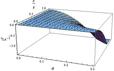
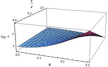
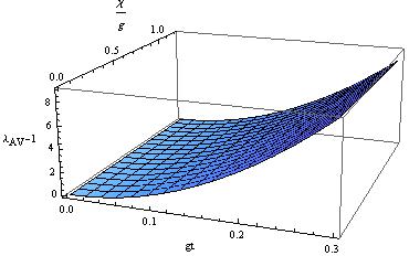
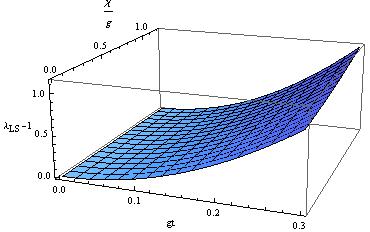
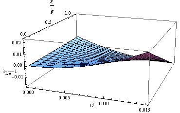
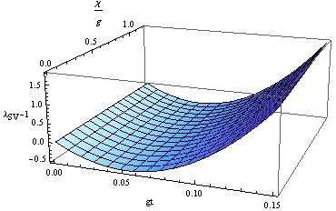
Figure 1: Variation of $\lambda_{ij}-1$ with respect to $p$ and $gt$ when $|\xi_{L}|=10,\,$ $|\xi_{A}|=1,$ $|\xi_{S}|=9$, $|\xi_{V}|=0.01$ and $\phi_{L}=\phi_{A}$.

3.3 Sub-shot noise

When we substitute (3) in (9) we find that

$$C_{LV}=-2p^{2}\tau^{2}I_{A}=2(K_{LV})_{\pm}$$ (14)

and

$$C_{SV}=-2\tau^{2}I_{A}=2(K_{SV})_{\pm}$$ (15)

and $C_{ij}=0$ in the remaining four cases. Since in this particular system $C_{LV}$ and $C_{SV}$ are directly proportional to $(K_{LV})_{\pm}$ and $(K_{SV})_{\pm}$, wherever we have seen intermodal entanglement we, can also observe sub-shot noise in those cases.

3.4 Variances

Using (3)-(5) and (10) we can obtain the analytic expressions for intermodal variances in the following forms

$$\begin{array}[]{lcl}\left\langle\left(\Delta W_{AV}\right)^{2}\right\rangle_{+}&=&2\tau^{2}I_{V}\left(I_{L}-p|\xi_{S}||\xi_{A}|\cos(\theta_{1}+\theta_{2})\right),\\ \left\langle\left(\Delta W_{SA}\right)^{2}\right\rangle_{+}&=&2\tau^{2}I_{L}\left(I_{S}-p|\xi_{S}||\xi_{A}|\cos(\theta_{2}-\theta_{1})\right),\\ \left\langle\left(\Delta W_{LA}\right)^{2}\right\rangle_{+}&=&-2p\tau^{2}I_{L}|\xi_{S}||\xi_{A}|\cos(\theta_{2}-\theta_{1}),\\ \left\langle\left(\Delta W_{LS}\right)^{2}\right\rangle_{+}&=&2p\tau^{2}I_{L}|\xi_{A}|\left(p|\xi_{A}|+|\xi_{S}|\cos(\theta_{2}-\theta_{1})\right),\\ \left\langle\left(\Delta W_{LV}\right)^{2}\right\rangle_{+}&=&2p^{2}\tau^{2}\left(3I_{L}I_{A}+3I_{A}I_{V}+I_{A}-I_{L}I_{V}\right)\\ &+&2p\tau^{2}|\xi_{S}||\xi_{A}|\left(I_{L}\cos(\theta_{2}-\theta_{1})+I_{V}\cos(\theta_{1}+\theta_{2})\right)+4p\tau|\xi_{A}||\xi_{L}||\xi_{V}|\cos(\theta_{1}),\\ \left\langle\left(\Delta W_{SV}\right)^{2}\right\rangle_{+}&=&2\tau^{2}\left(3I_{L}I_{S}+3I_{L}I_{V}+p^{2}I_{A}I_{V}+I_{L}-I_{S}I_{V}\right)\\ &+&2p\tau^{2}|\xi_{S}||\xi_{A}|\left(2I_{L}\cos(\theta_{2}-\theta_{1})-3I_{V}\cos(\theta_{1}+\theta_{2})\right)+4\tau|\xi_{L}||\xi_{S}||\xi_{V}|\cos(\theta_{2}),\end{array}$$ (16)

and

$$\begin{array}[]{lcl}\left\langle\left(\Delta W_{AV}\right)^{2}\right\rangle_{-}&=&2\tau^{2}I_{V}\left(I_{L}+2p^{2}I_{A}-p|\xi_{S}||\xi_{A}|\cos(\theta_{1}+\theta_{2})\right),\\ \left\langle\left(\Delta W_{SA}\right)^{2}\right\rangle_{-}&=&2\tau^{2}I_{L}\left(I_{S}+p|\xi_{S}||\xi_{A}|\cos(\theta_{2}-\theta_{1})\right),\\ \left\langle\left(\Delta W_{LA}\right)^{2}\right\rangle_{-}&=&2p\tau^{2}I_{L}\left(2pI_{A}-|\xi_{S}||\xi_{A}|\cos(\theta_{2}-\theta_{1})\right),\\ \left\langle\left(\Delta W_{LS}\right)^{2}\right\rangle_{-}&=&2\tau^{2}I_{L}\left(p^{2}I_{A}+2I_{S}-3p|\xi_{S}||\xi_{A}|\cos(\theta_{2}-\theta_{1})\right),\\ \left\langle\left(\Delta W_{LV}\right)^{2}\right\rangle_{-}&=&-2p^{2}\tau^{2}\left(I_{L}I_{A}+I_{A}I_{V}+I_{A}-I_{L}I_{V}\right)+4\tau^{2}I_{L}I_{V}\\ &-&6p\tau^{2}|\xi_{S}||\xi_{A}|\left(I_{L}\cos(\theta_{2}-\theta_{1})+I_{V}\cos(\theta_{1}+\theta_{2})\right)-4p\tau|\xi_{A}||\xi_{L}||\xi_{V}|\cos(\theta_{1}),\\ \left\langle\left(\Delta W_{SV}\right)^{2}\right\rangle_{-}&=&-2\tau^{2}\left(I_{L}I_{S}+I_{L}I_{V}-p^{2}I_{A}I_{V}+I_{L}-I_{S}I_{V}\right)\\ &-&2p\tau^{2}|\xi_{S}||\xi_{A}|\left(2I_{L}\cos(\theta_{2}-\theta_{1})-I_{V}\cos(\theta_{1}+\theta_{2})\right)-4\tau|\xi_{L}||\xi_{S}||\xi_{V}|\cos(\theta_{2}).\end{array}$$ (17)

Negativity of intermodal variances $\left\langle(\Delta W)_{ij}^{2}\right\rangle_{\pm}$ implies nonclassicality. Analytic expressions for intermodal variances $\left\langle(\Delta W)_{ij}^{2}\right\rangle_{+}$ and $\left\langle(\Delta W)_{ij}^{2}\right\rangle_{-}$ for all the possible combinations of modes in the stimulated Raman process are provided in (16) and (17), respectively. It is difficult to conclude directly about the presence of nonclassicality from these general analytic expressions of $\left\langle(\Delta W)_{ij}^{2}\right\rangle_{\pm}.$ Thus to visualize the existence of nonclassicality we have plotted the analytic expressions provided in (16) and (17). The plots are given in Fig. 2 and Fig. 3 and it is easy to see that both $\left\langle(\Delta W)_{ij}^{2}\right\rangle_{+}$ and $\left\langle(\Delta W)_{ij}^{2}\right\rangle_{-}$ depicts nonclassical behavior for a) pump and phonon mode and b) pump and anti-Stokes mode, c) Stokes and phonon mode. However for pump and Stokes mode only $\left\langle(\Delta W)_{LS}^{2}\right\rangle_{+}$ shows the existence of nonclassicality.

For the chosen values of $|\xi_{i}|$ and $p$ we have seen that $\left\langle(\Delta W)_{SA}^{2}\right\rangle_{\pm}=2\tau^{2}I_{L}|\xi_{S}|\left(|\xi_{S}|\pm p|\xi_{A}|\cos(\theta_{2}-\theta_{1})\right)>0$ but a negative value is possible if $p|\xi_{A}|>|\xi_{S}|$. Thus a very strong anti-Stokes coupling (compared to Stokes coupling) may yield nonclassical variance for Stokes and anti-Stokes mode. This is consistent with the appearance of intermodal squeezing where $\lambda_{AS}-1=I_{L}\tau^{2}(1-p)$ is negative only when $p>1,$ that is when anti-Stokes coupling is stronger than Stokes coupling.

Now from (17) we can easily observe that for a completely spontaneous Raman process $\left\langle(\Delta W)_{SV}^{2}\right\rangle_{-}=-2\tau^{2}I_{L}$ is always negative which indicates intermodal nonclassical behavior between phonon mode and Stokes mode. We have already shown that these two modes show intermodal entanglement, sub-shot noise behavior and squeezing of vacuum fluctuations in the spontaneous Raman process. Thus as far as the nonclassicalities in spontaneous Raman process are concerned these two modes play the most important role.

From (16) and (17) we can see that for very small values of rescaled time $\tau$ the term linear in $\tau$ is expected to dominate in $\left\langle(\Delta W)_{LV}^{2}\right\rangle_{\pm}$ and in $\left\langle(\Delta W)_{SV}^{2}\right\rangle_{\pm}$; $\left\langle(\Delta W)_{LV}^{2}\right\rangle_{\pm}$ varies with $\theta_{1}$, which is exhibited in Fig. 4. Further the linear term in $\left\langle(\Delta W)_{SV}^{2}\right\rangle_{+}$ is very weak and the nonclassical behavior can be seen only for a very small values of $\tau$. This is why in Fig. 2 we have plotted $\left\langle(\Delta W)_{SV}^{2}\right\rangle_{+}$ for a very short time only.

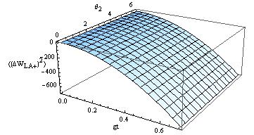
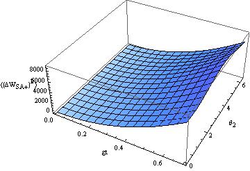
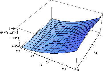
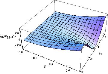
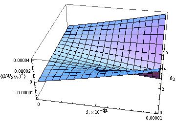
Figure 2: Variation of intermodal variance $\left\langle(\Delta W)_{ij}^{2}\right\rangle_{+}$ with respect to $gt$ and $\theta_{2}$ here we have chosen $|\xi_{L}|=10,\,$ $|\xi_{A}|=1,$ $|\xi_{S}|=9$, $|\xi_{V}|=0.01,\,$ $\theta_{1}=\frac{\pi}{6}$ and $p=0.9.$

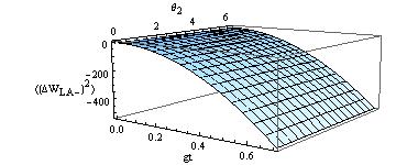
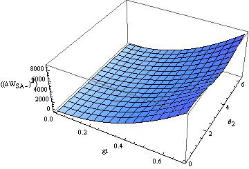
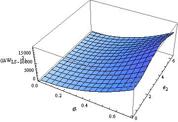
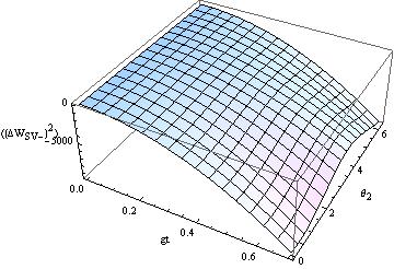
Figure 3: Variation of variance $\left\langle(\Delta W)_{ij}^{2}\right\rangle_{-}$ with respect to $gt$ and $\theta_{2}$ here we have chosen $|\xi_{L}|=10,\,$ $|\xi_{A}|=1,$ $|\xi_{S}|=9$, $|\xi_{V}|=0.01,\,$ $\theta_{1}=\frac{\pi}{6},$ and $p=0.9.$

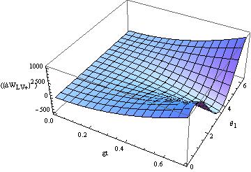
Figure 4: Variation of variance $\left\langle(\Delta W)_{LV}^{2}\right\rangle_{\pm}$ with respect to $\theta_{1}$ when $\theta_{2}=\frac{\pi}{6}$ all other parameters are same as in previous figures.

4 Phonon mode is chaotic

In this case we perform the average over the initial phonon amplitude in (2) with a Gaussian distribution in the Gaussian approximation. Assuming that the phonon mode is chaotic with average phonon number $\langle n_{V}\rangle,$ then the coefficients in the interaction picture described in (3) get modified as

$$\begin{array}[]{lcl}B_{L}&=&|\chi|^{2}t^{2}|\xi_{A}|^{2}\left(\langle n_{V}\rangle+1\right)+|g|^{2}t^{2}|\xi_{S}|^{2}\langle n_{V}\rangle,\\ B_{S}&=&|g|^{2}t^{2}|\xi_{L}|^{2}\left(\langle n_{V}\rangle+1\right),\\ B_{A}&=&|\chi|^{2}t^{2}|\xi_{L}|^{2}\langle n_{V}\rangle,\\ B_{V}&\approx&\langle n_{V}\rangle,\\ C_{L}&=&-g^{*}\chi t^{2}\xi_{A}\xi_{S}\left(2\langle n_{V}\rangle+1\right),\\ C_{S}&=&0,\\ C_{A}&=&0,\\ C_{V}&=&-g\chi t^{2}\xi_{S}^{*}\xi_{A},\\ D_{LS}&=&-\frac{1}{2}|g|^{2}t^{2}\xi_{L}\xi_{S}\left(2\langle n_{V}\rangle+1\right),\\ D_{LA}&=&-\frac{1}{2}|\chi|^{2}t^{2}\xi_{L}\xi_{A}\left(2\langle n_{V}\rangle+1\right),\\ D_{SA}&=&-\frac{1}{2}g\chi^{*}t^{2}\xi_{L}^{2}\left(2\langle n_{V}\rangle+1\right),\\ D_{SV}&=&igt\xi_{L}\left(\langle n_{V}\rangle+1\right),\\ D_{LV}&=&i\chi t\xi_{A}\left(\langle n_{V}\rangle+1\right),\\ D_{AV}&=&0,\\ \bar{D}_{LS}&=&-g\chi^{*}t^{2}\xi_{A}^{*}\xi_{L}\left(\langle n_{V}\rangle+1\right),\\ \bar{D}_{LA}&=&-g\chi^{*}t^{2}\xi_{S}^{*}\xi_{L}\langle n_{V}\rangle,\\ \bar{D}_{SA}&=&0,\\ \bar{D}_{SV}&=&0,\\ \bar{D}_{LV}&=&igt\xi_{S}^{*}\langle n_{V}\rangle,\\ \bar{D}_{AV}&=&i\chi t\xi_{L}^{*}\langle n_{V}\rangle.\end{array}$$ (18)

Now using equations (4), (5) and (18) we can obtain for single-mode variances

$$\begin{array}[]{lcl}\langle\left(\Delta W_{L}\right)^{2}\rangle_{N}&=&2p^{2}\tau^{2}I_{A}I_{L}\left(\langle n_{V}\rangle+1\right)+2\tau^{2}I_{S}I_{L}\langle n_{V}\rangle-2p\tau^{2}|\xi_{A}||\xi_{S}|I_{L}\left(2\langle n_{V}\rangle+1\right)\cos(\theta_{2}-\theta_{1}),\\ \langle\left(\Delta W_{S}\right)^{2}\rangle_{N}&=&2\tau^{2}I_{L}I_{S}\left(\langle n_{V}\rangle+1\right),\\ \langle\left(\Delta W_{A}\right)^{2}\rangle_{N}&=&2p^{2}\tau^{2}I_{L}I_{A}\langle n_{V}\rangle,\\ \langle\left(\Delta W_{V}\right)^{2}\rangle_{N}&\approx&\langle n_{V}\rangle^{2},\end{array}$$ (19)

and for correlation fluctuations

$$\begin{array}[]{lcl}\left(\Delta W_{L}\Delta W_{A}\right)_{N}&=&-\tau^{2}p^{2}I_{L}I_{A}\left(2\langle n_{V}\rangle+1\right)+2p\tau^{2}I_{L}|\xi_{S}||\xi_{A}|\langle n_{V}\rangle\cos(\theta_{2}-\theta_{1}),\\ \left(\Delta W_{L}\Delta W_{S}\right)_{N}&=&-\tau^{2}I_{L}I_{S}\left(2\langle n_{V}\rangle+1\right)+2p\tau^{2}I_{L}|\xi_{S}||\xi_{A}|\left(\langle n_{V}\rangle+1\right)\cos(\theta_{2}-\theta_{1}),\\ \left(\Delta W_{S}\Delta W_{A}\right)_{N}&=&-\tau^{2}pI_{L}|\xi_{A}||\xi_{S}|\cos(\theta_{2}-\theta_{1})\left(2\langle n_{V}\rangle+1\right).\end{array}$$ (20)

Analytic expressions of the other cross-correlations are not of interest as all variances that involve phonon mode will always be positive because of the dominance of $\langle\left(\Delta W_{V}\right)^{2}\rangle\approx\langle n_{V}\rangle^{2}$ term. Now substituting equations (18), (19) and (20) in the criteria of nonclassicalities introduced in (6)-(10) we can investigate the nonclassical character of stimulated and spontaneous Raman process when the phonon mode is chaotic and then compare the results with the similar results obtained in the coherent case. This is done in the following subsections.

4.1 Intermodal entanglement

Substituting (18) in (8) we obtain

$$\begin{array}[]{lcl}\left(K_{SV}\right)_{\pm}&=&-\tau^{2}I_{L}\left(\langle n_{V}\rangle+1\right),\\ \left(K_{LV}\right)_{\pm}&=&-p^{2}\tau^{2}I_{A}\left(\langle n_{V}\rangle+1\right)\mp 2p\tau^{2}|\xi_{A}||\xi_{S}|\langle n_{V}\rangle\left(3\langle n_{V}\rangle+2\right).\end{array}$$ (21)

All other $\left(K_{ij}\right)_{\pm}=0$.

We can conclude:

1. From (21) it is clear that the phonon mode is always entangled with Stokes mode. The same characteristic was also observed in coherent case but if we consider $\left(K_{SV}\right)_{\pm}$ as a measure of amount of entanglement, then the amount of entanglement in chaotic case is increased by a factor of $\left(1+\langle n_{V}\rangle\right)$ and it is more announced.

2. Similarly the phonon mode can be entangled with the pump mode. It is straightforward to see that $\left(K_{LV}\right)_{+}=-p^{2}\tau^{2}I_{A}\left(\langle n_{V}\rangle+1\right)-2p\tau^{2}|\xi_{A}||\xi_{S}|\langle n_{V}\rangle\left(\left(3\langle n_{V}\rangle+2\right)\right)$ exhibits intermodal entanglement.

3. But interestingly $\left(K_{LV}\right)_{-}$ does not show signature of intermodal entanglement.

4. Stokes mode and phonon mode are entangled for completely spontaneous Raman process also but the present calculation is non-conclusive about entanglement of pump and phonon mode.

4.2 Single mode and intermodal squeezing

By substituting (18) in (6) and (7) we obtain

$$\begin{array}[]{lcl}\lambda_{L}&=&1+2\tau^{2}\left[p^{2}I_{A}\left(\langle n_{V}\rangle+1\right)+I_{S}\langle n_{V}\rangle-p|\xi_{A}||\xi_{S}|\left(2\langle n_{V}\rangle+1\right)\right],\\ \lambda_{LA}&\approx&1+p^{2}\tau^{2}|\xi_{L}|\left(|\xi_{L}|\langle n_{V}\rangle-|\xi_{A}|\left(2\langle n_{V}\rangle+1\right)\right),\\ \lambda_{LS}&\approx&1+\tau^{2}|\xi_{L}|\left(|\xi_{L}|\left(\langle n_{V}\rangle+1\right)-|\xi_{S}|\left(2\langle n_{V}\rangle+1\right)\right),\\ \lambda_{SA}&=&1+\tau^{2}I_{L}(1-p)\left(\langle n_{V}\rangle+1-p\langle n_{V}\rangle\right).\end{array}$$ (22)

We see that:

1. Squeezing in the pump laser mode can be observed by approximating $\frac{|\xi_{A}|}{|\xi_{S}|}>\frac{\langle n_{V}\rangle}{\left(2\langle n_{V}\rangle+1\right)}$.

2. Intermodal squeezing is not possible when one of the mode is phonon mode as in that case $\lambda_{iV}\approx 1+\langle n_{V}\rangle>1.$

3. Intermodal squeezing will not be usually observed between pump mode and anti-Stokes mode as $\lambda_{LA}<1$ implies $|\xi_{L}|<2|\xi_{A}|+\frac{|\xi_{A}|}{\langle n_{V}\rangle}\approx 2|\xi_{A}|$. But technically it is allowed and intermodal squeezing between pump mode and anti-Stokes mode can in principle be seen for stimulated Raman process as well as for partially spontaneous Raman process ($I_{A}\neq 0$, $I_{L}\neq 0$, $I_{S}=0$,   $I_{V}=0$).

4. Intermodal squeezing between pump mode and Stokes mode is possible if $|\xi_{L}|\left(\langle n_{V}\rangle+1\right)<|\xi_{S}|\left(2\langle n_{V}\rangle+1\right),$ i.e. if $\frac{|\xi_{L}|}{|\xi_{S}|}<\frac{\left(2\langle n_{V}\rangle+1\right)}{\left(\langle n_{V}\rangle+1\right)}$. For $\langle n_{V}\rangle\gg 1$ this condition implies that $|\xi_{L}|<2|\xi_{S}|$ and for $\langle n_{V}\rangle=0$ it implies $|\xi_{L}|<|\xi_{S}|.$

5. To have $\lambda_{SA}<1,$ we need $p=\frac{|\chi|}{|g|}>1$ and $\left(\langle n_{V}\rangle+1\right)>p\langle n_{V}\rangle,$ i.e. $\frac{|\chi|}{|g|}<1+\frac{1}{\langle n_{V}\rangle}.$ For coherent scattering $\langle n_{V}\rangle\rightarrow 0$ and we have the previous condition $\frac{|\chi|}{|g|}>1.$

6. Similarly when $p<1$ then $\lambda_{SA}<1$ implies $\left(p\langle n_{V}\rangle-\left(\langle n_{V}\rangle+1\right)\right)>0\Rightarrow p>1+\frac{1}{\langle n_{V}\rangle}\Rightarrow p>1$. Thus the condition of negativity is not satisfied and we are non-conclusive about the entanglement between Stokes mode and anti-Stokes mode if $p<1.$

4.3 Sub-shot noise

By substituting (18) in (9) we obtain

$$\begin{array}[]{lcl}C_{AV}&=&\langle n_{V}\rangle^{2}\left(1-2p^{2}\tau^{2}I_{L}\right),\\ C_{LV}&=&\langle n_{V}\rangle^{2}-2p^{2}\tau^{2}I_{A}\left(\langle n_{V}\rangle+1\right)^{2}-2\tau^{2}I_{S}\langle n_{V}\rangle^{2},\\ C_{SV}&=&\langle n_{V}\rangle^{2}-2\tau^{2}I_{L}\left(\langle n_{V}\rangle+1\right)^{2},\end{array}$$ (23)

and all other $C_{ij}=0.$ For stimulated Raman process, sub-shot noise is observed in the above three cases. In coherent case subshot noise behavior was not observed for anti-Stokes and phonon mode. Further, negativity of $C_{AV}$ and $C_{SV}$ will be observed for spontaneous Raman process too. But in the spontaneous Raman process sub-shot noise behavior will not be observed for pump and phonon modes. However, we can observe it for partially spontaneous process ($\langle n_{V}\rangle\neq 0,\,I_{L}\neq 0,\,I_{A}=0$ and $I_{S}=0$.)

4.4 Variances

By substituting (19) and (20) in (10) we obtain

$$\begin{array}[]{lcl}\langle\left(\Delta W\right)_{SA}^{2}\rangle_{\pm}&=&2p^{2}\tau^{2}I_{L}I_{A}\langle n_{V}\rangle+2\tau^{2}I_{L}I_{S}\left(\langle n_{V}\rangle+1\right)\\ &\mp&2\tau^{2}pI_{L}|\xi_{A}||\xi_{S}|\cos(\theta_{2}-\theta_{1})\left(2\langle n_{V}\rangle+1\right),\\ \langle\left(\Delta W\right)_{LS}^{2}\rangle_{\pm}&=&2p^{2}\tau^{2}I_{A}I_{L}\left(\langle n_{V}\rangle+1\right)+2\tau^{2}I_{L}I_{S}\left(2\langle n_{V}\rangle+1\right)(1\mp 1)\\ &-&2p\tau^{2}I_{L}|\xi_{S}||\xi_{A}|\cos(\theta_{2}-\theta_{1})\left(\left(2\langle n_{V}\rangle+1\right)\mp 2\left(\langle n_{V}\rangle+1\right)\right),\\ \langle\left(\Delta W\right)_{LA}^{2}\rangle_{\pm}&=&2p^{2}\tau^{2}I_{A}I_{L}\left(\left(2\langle n_{V}\rangle+1\right)\mp\left(\langle n_{V}\rangle+1\right)\right)+2\tau^{2}I_{S}I_{L}\langle n_{V}\rangle\\ &-&2p\tau^{2}|\xi_{A}||\xi_{S}|I_{L}\cos(\theta_{2}-\theta_{1})\left(\left(2\langle n_{V}\rangle+1\right)\mp 2\langle n_{V}\rangle\right).\end{array}$$ (24)

From (24) we observe following:

1. $\langle\left(\Delta W\right)_{LS}^{2}\rangle_{+}=2p\tau^{2}|\xi_{A}|I_{L}\left(p|\xi_{A}|\left(\langle n_{V}\rangle+1\right)+|\xi_{S}|\cos(\theta_{2}-\theta_{1})\right)$. Thus negative variance can be seen for $p|\xi_{A}|\left(\langle n_{V}\rangle+1\right)<|\xi_{S}|$. Since $|\xi_{A}|<|\xi_{S}|$ this nonclassical feature between pump mode and Stokes mode will be observed for small values of mean phonon number $\langle n_{V}\rangle.$

2. In the analytic expression of $\langle\left(\Delta W\right)_{AS}^{2}\rangle_{\pm}$ if we assume $I_{A}\ll I_{S}$ then we obtain

   $$\langle\left(\Delta W\right)_{AS}^{2}\rangle_{\pm}=2\tau^{2}I_{L}|\xi_{S}|\left(|\xi_{S}|\left(\langle n_{V}\rangle+1\right)\mp p|\xi_{A}|\left(2\langle n_{V}\rangle+1\right)\cos(\theta_{2}-\theta_{1})\right)$$

   which would show nonclassicality if $p\frac{|\xi_{A}|}{|\xi_{S}|}>\frac{\langle n_{V}\rangle+1}{2\langle n_{V}\rangle+1}$. This implies $p|\xi_{A}|>\frac{1}{2}|\xi_{S}|$ which is inconsistent with the assumption $I_{A}\ll I_{S}$. Thus if $I_{A}\ll I_{S}$ then we do not observe nonclassical variance in anti-Stokes and Stokes modes.

3. If we assume $I_{A}\gg I_{S}$ and consider the complete analytic expression of $\langle\left(\Delta W_{AS}\right)^{2}\rangle_{\pm},$ then the condition $p\frac{|\xi_{A}|}{|\xi_{S}|}>\frac{\langle n_{V}\rangle+1}{2\langle n_{V}\rangle+1}$ will serve as necessary but not sufficient condition of nonclassicality. Now if we assume that for some choice of $p,I_{A},I_{S},\langle n_{V}\rangle$ we observe nonclassical intermodal variance for Stokes and anti-Stokes modes, then we can show that for that situation $\langle\left(\Delta W_{LS}\right)^{2}\rangle_{+}$ will not show nonclassicality. The proof is simple. First we assume that both $\langle\left(\Delta W_{LS}\right)^{2}\rangle_{+}$ and $\langle\left(\Delta W_{AS}\right)^{2}\rangle_{\pm}$ are negative. Therefore, $\frac{1}{\langle n_{V}\rangle+1}>p\frac{|\xi_{A}|}{|\xi_{S}|}>\frac{\langle n_{V}\rangle+1}{2\langle n_{V}\rangle+1}$, which implies $\left(2\langle n_{V}\rangle+1\right)>\left(\langle n_{V}\rangle+1\right)^{2}$ or $\langle n_{V}\rangle^{2}<0$. Thus by reductio ad absurdum we have shown that intermodal nonclassical variance cannot be seen simultaneously in a) Stokes and anti-Stokes mode and b) Stokes and pump mode.

4. For the compound mode $(LA)$ one could observe sub-shot noise provided that $|\chi||\xi_{A}|>\frac{|g||\xi_{S}|}{\sqrt{2}}.$

5 Joint photon-phonon number and wave distribution

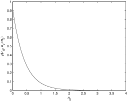
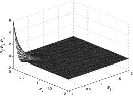
Figure 5: a) Joint photon-phonon number distribution for Stokes and vibration modes (left) and b) Quasi-distribution of integrated-intensities for the same modes (right). Here $B_{S}=0.1,\,B_{L}=0.01,\,B_{V}=0.11$ and $s=0.7.$

We can illustrate the above results for nonclassical behavior of modes in Raman scattering by joint photon-phonon number and integrated-intensity distributions along the lines given in [6] (and references therein) in Gaussian approximation. For simplicity we consider scattering by phonon vacuum (in optical region and for room temperature $\langle n_{V}\rangle\approx 0$) for compound modes $(SV$ ) and $(LV)$, which exhibit quantum entanglement up to the second order in $t$. From (3) we see that $K_{SV}=-B_{S}=-B_{V}=-|g|^{2}t^{2}I_{L}$ provided that we consider spontaneous scattering $(I_{A}=I_{S}=0;$ in this case $C_{S}=C_{V}=\bar{D}_{SV}=0).$ In principle we can also consider partially stimulated scattering with $I_{S}\neq 0,$ when using shifted distributions in $W_{S}$ along $I_{S}$ [7] to adopt spontaneous process. Thus $K_{SV}+B_{S}=K_{SV}+B_{V}=0$ and from the formulae given in [6] we obtain the joint photon-phonon number distribution

$$p(n_{S},n_{V})=\frac{(B_{S})^{n_{S}}}{(1+B_{S})^{1+n_{S}}}\delta_{n_{S},n_{V}},$$ (25)

i.e. it is diagonal expressing a pairwise structure of photon-phonon process in this case. It is shown in Fig. 5a. The corresponding $s$-order quasidistribution of integrated-intensities is [6]

$$P_{s}\left(W_{S},W_{V}\right)=\frac{1}{\pi B_{Ss}}{\rm e}^{-\frac{W_{S}+W_{V}}{2B_{Ss}}}\frac{\sin\left(\frac{W_{S}-W_{V}}{\sqrt{-K_{VS,s}}}\right)}{W_{S}-W_{V}},$$ (26)

where $B_{Ss}=B_{S}+\frac{1-s}{2}$ and $K_{SV,s}=K_{SV}+(1-s)B_{S}+\frac{(1-s)^{2}}{4};$ $s$ is ordering parameter. For the threshold value of the ordering parameter we have $s_{th}=1+B_{S}+B_{V}-\sqrt{(B_{S}+B_{V})^{2}-4K_{SV}}\approx 1+2B_{S}-2\sqrt{B_{S}}.$ Choosing $|g|t=0.1,\,I_{L}=10,$ we have $s_{th}=0.57.$ So we calculate the quasi-distribution for $s=0.7;$ in this case $B_{S}=0.1,$ $B_{Ss}=0.25,$ $K_{VS,s}=-0.048.$ This quasi-distribution is shown in Fig. 5b. It takes on negative values exhibiting nonclassical oscillations and behavior.

Similarly, we can treat the compound mode $(LV)$ considering again photon vacuum scattering with partial stimulation $I_{A}\neq 0$ and $I_{S}=0.$ Shifting distribution in $W_{L}$ along $I_{L}$ and neglecting short-time terms as above we obtain from (3), $K_{LV}=-|\chi|^{2}t^{2}I_{A}=-B_{L}$ and $B_{V}=|g|^{2}t^{2}I_{L}+|\chi|^{2}t^{2}I_{A},$ i.e. $K_{LV}+B_{L}=0$ and $K_{LV}+B_{V}=|g|^{2}t^{2}I_{L}>0$ ($C_{L}=C_{V}=\bar{D}_{LV}=0$). Thus for the joint photon-phonon number distribution [6] we obtain

$$p(n_{L},n_{V})=\frac{n_{V}!}{n_{L}!(n_{V}-n_{L})!}\frac{(B_{V}+K_{LV})^{n_{V}-n_{L}}}{(1+Bn_{V})^{n_{V}+1}},\,n_{V}\geq n_{L}.$$ (27)

For $n_{V}<n_{L},$ the distribution is zero. Its quantum behavior is illustrated in Fig. 6a, showing one-side behavior along the diagonal compared to the earlier cases [7]. For the threshold values of the ordering parameter we have $s_{th}\approx 1+|g|^{2}t^{2}I_{L}-2|\chi|t\sqrt{I_{A}}.$ Assuming for simplicity $|\chi|=|g|,\,I_{A}=1$ and $I_{L}=10,$ we have $s_{th}=0.9$ and nonclassical behavior of wave quasi-distribution is illustrated by the Glauber-Sudarshan quasi-distribution of integrated-intensities for $s=1$:

$$P_{N}(W_{L},W_{V})=\frac{1}{\pi\sqrt{B_{L}B_{V}}}{\rm e}^{-\frac{W_{L}}{2B_{L}}-\frac{W_{V}}{2B_{V}}}\frac{\sin\left[\frac{\sqrt{\frac{B_{V}}{B_{L}}}W_{L}-\sqrt{\frac{B_{L}}{B_{V}}}W_{V}}{\sqrt{B_{L}}}\right]}{\sqrt{\frac{B_{V}}{B_{L}}}W_{L}-\sqrt{\frac{B_{L}}{B_{V}}}W_{V}},$$ (28)

as shown in Fig. 6b. The existence of nonclassical character is clearly visible through the negative values of $P_{N}(W_{L},W_{V}).$

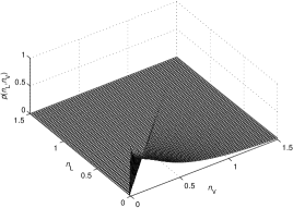
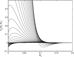
Figure 6: a) Joint photon-phonon number distribution for pump and vibration modes (left) and b) Glauber-Sudarshan quasi-distribution of integrated-intensities for the same modes with $W_{V}=0,\,0.1,\,0.2.\cdots 2$ (right).

6 Difference and conditional number distributions

In this section we can further illustrate the observed nonclassicalities via difference and conditional number distributions. For example, nonclassical character associated with a mode can be illustrated using conditional Fano factor, which is defined as

$$F_{i,C}=\frac{\left\langle(\Delta n_{i})^{2}\right\rangle_{C}}{\left\langle n_{i}\right\rangle},$$

for mode $i$. Corresponding condition for nonclassicality is $F_{i,C}<1.$ Analytic expressions for conditional Fano factor are obtained here for modes of interest (i.e. for $F_{L,C}$ and $F_{V,C}$) as follows:

$$F_{L,C}=1-\frac{B_{L}}{B_{V}},$$ (29)

and

$$F_{V,C}=\frac{(n_{L}+1)\left(\frac{1+B_{V}}{1+B_{L}}\right)^{2}-1}{(n_{L}+1)\left(\frac{1+B_{V}}{1+B_{L}}\right)-1}-1.$$ (30)

It is now easy to observe from (3) that $B_{L}$ and $B_{V}$ are always positive, consequently the conditional Fano factor $F_{L,C}$ is always less than unity. Thus conditional Fano factor always depicts nonclassicality in pump mode. However, in phonon mode the presence of nonclassicality (i.e. $F_{V,C}<1$) is not directly visible from the expression, but the same is shown in the Fig. 7.

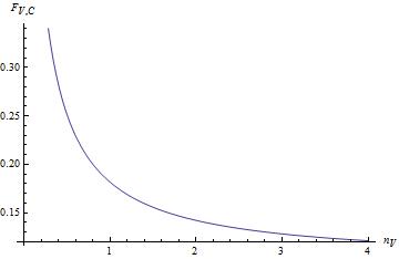
Figure 7: Conditional Fano factor $F_{V,C}$ for phonon mode shows nonclassical behavior as $F_{V,C}<1$. Here $B_{V}=0.11$ and $B_{L}=0.01,$ $K_{LV}=-0.01$.

The corresponding number distributions are obtained as

$$\begin{array}[]{lcl}p_{C}\left(n_{L};n_{V}\right)&=&\frac{n_{V}!}{n_{L}!\left(n_{V}-n_{L}\right)!}\left(1-\frac{B_{L}}{B_{V}}\right)^{n_{V}}\left(\frac{B_{L}}{B_{V}-B_{L}}\right)^{n_{L}},\\ p_{C}\left(n_{V};n_{L}\right)&=&\frac{n_{V}!}{n_{L}!\left(n_{V}-n_{L}\right)!}\frac{1+B_{L}}{1+B_{V}}\left(\frac{B_{V}-B_{L}}{1+B_{V}}\right)^{n_{V}}\left(\frac{1+B_{L}}{B_{V}-B_{L}}\right)^{n_{L}}.\end{array}$$ (31)

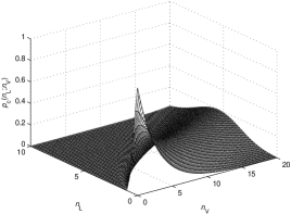
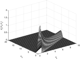
Figure 8: Conditional number distributions $p_{C}\left(n_{L};n_{V}\right)$ (left) and $p_{C}\left(n_{V};n_{L}\right)$ (right). Here $B_{V}=0.11$ and $B_{L}=0.01,$ $K_{LV}=-0.01$.

These conditional number distributions are plotted in the Fig. 8. Difference number distribution can be obtained as

$$p_{-}(n)=\frac{\left(B_{V}-B_{L}\right)^{n}}{\left(1+B_{V}-B_{L}\right)^{n+1}},$$ (32)

$$\langle\left(\Delta n\right)^{2}\rangle_{-}=\left(B_{V}-B_{L}\right)\left(1+B_{V}-B_{L}\right)$$

and Poissonian distribution for the same two modes is

$$p_{Pois}(n)=\frac{\left(B_{V}+B_{L}\right)^{n}}{n!}{\rm e}^{-\left(B_{V}+B_{L}\right).}$$ (33)

A joint plot of $p_{-}(n)$ and $p_{pois}(n)$ is provided in Fig. 9, which clearly shows subpoissonian character in $p_{-}(n)$. Thus a nonclassical difference number distribution is observed. For the sub-shot noise parameter $R=\frac{\langle\left(\Delta n_{ij}\right)^{2}\rangle}{\left(\langle n_{i}\rangle+\langle n_{j}\rangle\right)}$ we have $R\thickapprox 1-\frac{2B_{L}}{B_{L}+B_{V}}=0.83<1.$

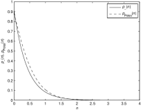
Figure 9: Difference number distribution $p_{-}(n)$ and $p_{pois}(n)$. Subpoissonian character is shown by $p_{-}(n)$. Here $B_{V}=0.11$ and $B_{L}=0.01,$ $K_{LV}=-0.01$.

7 Conclusion

We have observed different type of nonclassicalities in the stimulated, completely spontaneous and partially spontaneous Raman process. The observations that are discussed in detail in Section 3.1 are summarized in Table 1 for coherent scattering. We see that in general various nonclassical features of the process can or cannot be directly related, only for combined modes $(LV)$ and $(SV)$ all of them occurs simultaneously. We have not restricted ourselves to the study of coherent scattering alone. In Section 4 we have investigated various nonclassical characters of Raman process when the phonon mode is chaotic. Finally we have illustrated our results by joint photon-phonon number and wave distributions.

Mode	$E_{ij}$	$\lambda_{ij}$	$C_{ij}$	$\left\langle\left(\Delta W_{ij}\right)^{2}\right\rangle_{-}$	$\left\langle\left(\Delta W_{ij}\right)^{2}\right\rangle_{+}$	$(K_{ij})_{+}$	$(K_{ij})_{-}$
AV	non-conclusive	>1	non-conclusive	+ve	+ve	non-conclusive	non-conclusive
AL	non-conclusive	<1 if $I_{L}>I_{A}$ (expected)	non-conclusive	-ve region exists	-ve region exists	non-conclusive	non-conclusive
AS	non-conclusive	<1 if $|\chi|>|g|$	non-conclusive	+ve	+ve	non-conclusive	non-conclusive
LS	non-conclusive	>1	non-conclusive	+ve	-ve region exists	non-conclusive	non-conclusive
LV	always -ve	< for short time	always -ve	-ve region exists	-ve region exists	always -ve	always -ve
SV	always -ve	< for short time	always -ve	-ve	-ve	always -ve	always -ve

Table 1: Negativity of different characteristics of nonclassicality. Here we have used $E_{ij}=B_{i}B_{j}-|\bar{D}_{ij}|^{2},$ $\lambda_{ij}=1+B_{i}+B_{j}-2{\rm Re}\bar{D}_{ij}-|C_{i}+C_{j}+2D_{ij}|<1,$ $C_{ij}=B_{i}^{2}+B_{j}^{2}+|C_{i}|^{2}+|C_{j}|^{2}-2|D_{ij}|^{2}-2|\bar{D}_{ij}|^{2}<0,$ $\left(K_{ij}\right)_{\pm}=(B_{i}\pm|C_{i}|)(B_{j}\pm|C_{j}|)-\left(|D_{ij}|\mp|\bar{D}_{ij}|\right)^{2}.$

Acknowledgment: A. P. thanks Department of Science and Technology (DST), India for support provided through the DST project No. SR/S2/LOP-0012/2010. He also thanks the Operational Program Education for Competitiveness - European Social Fund project CZ.1.07/2.3.00/20.0017 of the Ministry of Education, Youth and Sports of the Czech Republic. J. P. and J. K. thank the Operational Program Research and Development for Innovations - European Regional Development Fund project CZ.1.05/2.1.00/03.0058 of the Ministry of Education, Youth and Sports of the Czech Republic.

References

- [1] B. Sen, V. A. , J. and J. , J. Phys. B 44 (2011) 105503.
- [2] B. Sen, S. Mandal and J. , J. Phys. B: At. Mol. Opt. Phys. 40 (2007) 1417.
- [3] J. , Quantum Statistics of Linear and Nonlinear Optical Phenomena, Dordrecht, Kluwer (1991).
- [4] A. Miranowicz and S. Kleich, Modern Nonlinear Optics, Vol. 3, Eds. M. W. Evans and S. Kleich, J. Wiley, New York (1994), pp. 531-626.
- [5] D. F. Walls, Z. Phys. 237 (1970) 224.
- [6] J. and J. , Opt. Commun. 284 (2011) 4941.
- [7] J. and J. , Opt. Commun. 256 (2006) 632.